On the accuracy of the MB-pol many-body potential for water: Interaction energies, vibrational frequencies, and classical thermodynamic and dynamical properties from clusters to liquid water and ice.

Abstract

The MB-pol many-body potential has recently emerged as an accurate molecular model for water simulations from the gas to the condensed phase. In this study, the accuracy of MB-pol is systematically assessed across the three phases of water through extensive comparisons with experimental data and high-level ab initio calculations. Individual many-body contributions to the interaction energies as well as vibrational spectra of water clusters calculated with MB-pol are in excellent agreement with reference data obtained at the coupled cluster level. Several structural, thermodynamic, and dynamical properties of the liquid phase at atmospheric pressure are investigated through classical molecular dynamics simulations as a function of temperature. The structural properties of the liquid phase are in nearly quantitative agreement with X-ray diffraction data available over the temperature range from 268 to 368 K. The analysis of other thermodynamic and dynamical quantities emphasizes the importance of explicitly including nuclear quantum effects in the simulations, especially at low temperature, for a physically correct description of the properties of liquid water. Furthermore, both densities and lattice energies of several ice phases are also correctly reproduced by MB-pol. Following a recent study of DFT models for water, a score is assigned to each computed property, which demonstrates the high and, in many respects, unprecedented accuracy of MB-pol in representing all three phases of water.

I Introduction

Fast, reliable, and accurate modeling of structural, physical, and chemical properties of water across all media - gas, liquid, interface, confined and solid - and at different thermodynamic conditions is a long-standing challenge. This is largely because the quality of any theoretical prediction depends heavily on the underlying intermolecular potential energy surface (PES) utilized.Cisneros et al. (2016); Bukowski et al. (2007); Cencek et al. (2008); Vega and Abascal (2011) While in principle, ab initio molecular dynamics (AIMD) simulations carried out with correlated electronic structure methods can provide a correct description of water across all phases, these simulations are currently unfeasible due to the prohibitive associated computational cost. Despite recent progress in the development and implementation of simulation approaches based on Möller-Plesset perturbation theory, density functional theory (DFT) still remains the most common approach used in ab initio simulations of water.Marx and Hutter (2009); Car and Parrinello (1985); Schlegel et al. (2002); Payne et al. (1992) However, existing functionals have been shown to remain limited in the accuracy and predictive ability with which they can represent the properties of water in different phases.Gillan et al. (2016)

On the other hand, empirical water models based on molecular mechanics (commonly referred to as force fields) have been used extensively in computer simulations to investigate the properties of water under different thermodynamic conditions. In these models, the force field parameters are usually tuned to reproduce a (limited) set of experimental properties.Guillot (2002); Shvab and Sadus (2016); Abascal and Vega (2005); Horn et al. (2004); Jorgensen et al. (1983); Mahoney and Jorgensen (2000); Berendsen et al. (1987); Vega et al. (2009); Vega and Abascal (2011) The most common empirical models are pairwise additive, assume the water molecules to be rigid, and use fixed point charges to describe the electrostatic interactions. Despite their simplicity, empirical models have had great success in reproducing, at least to some extent, structural, thermodynamic, and transport properties of liquid water over a broad range of temperatures and pressures.Abascal and Vega (2005); Horn et al. (2004); Guillot (2002); Jorgensen et al. (1983); Mahoney and Jorgensen (2000); Berendsen et al. (1987); Vega et al. (2009); Vega and Abascal (2011) Examples under this category include RWK,Reimers et al. (1982) SPC,Berendsen et al. (1981) SPC/E,Berendsen et al. (1987) TIP4P,Jorgensen et al. (1983) TIP4P-2005,Abascal and Vega (2005) TIP4P-Ew,Horn et al. (2004) and TIP5P.Mahoney and Jorgensen (2000) The reader is referred to Refs. 4, 10 and 11 as well as the original studies for complete details of rigid water models. Flexible versions were also developed for some of these water models to investigate vibrational dynamics and energy transfer in the liquid phase.Habershon et al. (2009); Paesani et al. (2006) To go beyond the pairwise approximation, several water models have been developed which include either empirical three-body terms (e.g., E3BKumar and Skinner (2008); Tainter et al. (2011, 2015)) or implicit many-body effects through classical polarization (e.g., BK3,Kiss and Baranyai (2013) SWM4-DP,Lamoureux et al. (2003) SWM4-NDP,Lamoureux et al. (2006) SWM6,Yu et al. (2013) COS,Yu et al. (2003); Yu and van Gunsteren (2004); Kiss and Baranyai (2013) TTMx-F,Fanourgakis and Xantheas (2006, 2008); Burnham et al. (2008) AMOEBA,Ren and Ponder (2003); Ponder et al. (2010); Wang et al. (2013); Laury et al. (2015) GEM*,Duke et al. (2014) and POLY2VSHasegawa and Tanimura (2011)). The interested reader is referred to Ref. 1 for a systematic overview of recent water models.

While water models parameterized to reproduce experimental data have been instrumental in gaining qualitative insights into the behavior of liquid water, the lack of chemical accuracy results in limited predictive power across the entire phase diagram. Over the years, this has stimulated the development of analytical potential energy functions, originally introduced by Clementi and co-workers in the 1970s, which aim at representing the multidimensional potential energy surface (PES) associated with a system containing N water molecules through a rigorous representation of the many-body expansion (MBE) of the interaction energy,Hankins et al. (1970)

$$E_{\text{N}}=\sum_{i=1}^{N}V^{\text{1B}}(i)+\sum_{i<j}^{N}V^{\text{2B}}(i,j)+\sum_{i<j<k}^{N}V^{\text{3B}}(i,j,k)+\dots+V^{\text{NB}}(1,\dots,N),$$ (1)

where $V^{\text{1B}}$ is the one-body (1B) contribution corresponding to the deformation energy and the $V^{\text{nB}}$ are the n-body (nB) interaction energies defined as

$$\begin{split}V^{\text{nB}}=\quad&E_{n}(1,\dots,n)-\sum_{i}V^{\text{1B}}(i)-\sum_{i<j}V^{\text{2B}}(i,j)-\dots\\ &-\sum_{i<j<\dots<n-1}V^{\text{(n-1)B}}(i,j,\dots,(n-1)).\end{split}$$ (2)

Depending on the specific functional form adopted and the extent of the training sets used to fit the individual terms of the MBE, many-body potentials can approach the same level of accuracy as high-level correlated electronic structure calculations at a fraction of the computational cost.Medders et al. (2013) The most notable many-body potential energy functions are CC-pol,Bukowski et al. (2008a, b); Cencek et al. (2008); Góra et al. (2014); Szalewicz et al. (2009); Bukowski et al. (2007) WHBB,Wang et al. (2011); Huang et al. (2006); Wang and Bowman (2011); Wang et al. (2009); Wang and Bowman (2010) HBB2-pol,Babin et al. (2012); Medders et al. (2013); Babin and Paesani (2013) and MB-pol.Babin et al. (2013, 2014); Medders et al. (2014); Medders and Paesani (2015a) To date, MB-pol (and its precursor HBB2-pol) is the only many-body potential that has been consistently employed in molecular simulations, with explicit inclusion of nuclear quantum effects (NQE), which correctly reproduce the properties of water from the gas to the liquid and solid phases. Babin et al. (2012); Babin and Paesani (2013); Babin et al. (2013, 2014); Medders et al. (2014); Medders and Paesani (2015a); Medders et al. (2015); Medders and Paesani (2015b); Medders and Paesani (2016); Straight and Paesani (2016)

The purpose of this study is to systematically assess the accuracy of MB-pol in predicting structural, thermodynamic, dynamical, and spectroscopic properties of water across all phases as well as to provide a metric by which these properties can be compared to experiment. The article is organized as follows. Section II describes the technical details of all calculations and simulations employed in this study. Section III reports the results on several physical properties of water in the three phases: gas, liquid, and solid. The overall performance of MB-pol is then discussed by assigning a score to each computed property. The last section summarizes the results and provides an outlook of future applications of MB-pol.

II Methodology and Computational details

As discussed in detail in previous studies,Medders et al. (2013); Babin et al. (2013, 2014); Medders et al. (2014); Medders and Paesani (2015a) the MB-pol potential is built upon the MBE of Eq. 1 and includes explicit terms that describe 1B, 2B, and 3B terms, along with classical N-body polarization to account for all higher-body contributions to the interaction energy. The polarization term is represented by a slightly modified version of the Thole-type model as introduced in the TTM4-F model.Burnham et al. (2008) The 1B term is represented by the spectroscopically accurate water monomer PES developed by Partridge and Schwenke.Partridge and Schwenke (1997) The 2B term is further divided into long-range and short-range interactions and is described using classical electrostatics, induction, and dispersion forces, which dominate the long-range part, supplemented by a set of multivariable polynomials in the short-range, to capture the more complex quantum mechanical effects arising from the overlap of monomer electron densities. Along the same lines, the 3B term is composed of 3B induction and a multi-dimensional function to accurately describe both long-range and short-range interactions. The polynomial functions used to describe the short-range 2B and 3B interactions are generated in such a way that they retain permutational invariance with respect to the hydrogen atoms within the same water molecule as well as to whole water molecules within all possible dimers and trimers. The permutationally invariant polynomials are trained to a large set of highly accurate correlated coupled-cluster energies via a supervised machine learning approach. Specific details about the functional form, training sets, and training algorithms can be found in the original studies.Babin et al. (2012); Medders et al. (2013); Babin et al. (2013, 2014); Medders et al. (2014); Medders and Paesani (2015a) MB-pol is publicly available as an external pluginMBp (a) for the OpenMM toolkit for molecular simulationsEastman et al. (2013) and has recently been interfacedMBp (b) to the i-PI wrapper.Ceriotti et al. (2014)

All electronic structure calculations of water clusters presented in the next sections were carried out using MOLPRO.Werner et al. (2012) The reference interaction energies for (H₂O)${}_{\text{n}}$ clusters, with n = 4$-$6, optimized at the RI-MP2 and MP2 levels of theory in Refs. 67 and 68, were obtained using the MBE of the interaction energyHankins et al. (1970) as described in Ref. 69, with individual MB contributions calculated with the CCSD(T)/CCSD(T)-F12b method in the complete basis set (CBS) limit.Hill et al. (2009); Neese and Valeev (2011) The 2B interaction energies were computed at the CCSD(T) level of theory by extrapolating the values obtained with aug-cc-pVTZ and aug-cc-pVQZ basis sets supplemented with an additional set of (3s, 3p, 2d, 1f) midbond functions, with exponents equal to (0.9, 0.3, 0.1) for s and p orbitals, (0.6, 0.2) for d orbitals, and 0.3 for f orbitals, placed at the center of mass of each dimer configuration.Dunning Jr (1989); Kendall et al. (1992); Tao and Pan (1992) The following two-point formulaHalkier et al. (1999a, b) was used to extrapolate the interaction energies to the CBS limit:

$$\text{V}_{\text{2B}}^{\text{X}}=\text{V}_{\text{2B}}^{\text{CBS}}-\frac{\text{A}}{\text{X}^{\text{3}}}$$ (3)

with cardinal numbers X = 3 and 4, accordingly. The Hartree–Fock energy was not extrapolated separately since it was close to the CBS limit for either value of X. The 3B interaction energies were calculated at the CCSD(T) level of theory using the aug-cc-pVTZ basis set supplemented with the same set of midbond functions introduced above, which were placed at the center of mass of each trimer configuration. All higher ($>$3B) contributions were computed with the CCSD(T)-F12 method using the VTZ-F12 basis sets.Adler et al. (2007); Peterson et al. (2008); Knizia et al. (2009) This method yields results close to the CBS values at lower computational cost than direct CCSD(T) calculations with large basis sets.Tew et al. (2007); Bischoff et al. (2009) All 3B and higher-body energies were corrected for the basis set superposition error (BSSE) using the counterpoise method.Boys and Bernardi (1970)

The MB-pol vibrational frequencies of the water clusters were calculated within the harmonic approximation from the diagonalization of the mass-weighted Hessian matrix. Each cluster structure was first energy minimized until the norm of the force vector reached a value smaller than 10^-8 kcal mol${{}^{\raisebox{0.60275pt}{$\scriptscriptstyle-1$}}}$ Å^-1. The absence of any imaginary frequencies indicates that all structures reported in Section III.1.2 correspond to either a local or a global minimum.

All molecular dynamics (MD) simulations of liquid water presented in the next sections were carried out at the classical level using in-house software based on the DL_POLY_2 simulation package,Smith and Forester (1996) which was modified to include the MB-pol potential.Medders et al. (2014) Unless otherwise stated, the systems consisted of 256 water molecules placed in a cubic simulation box. The velocity-Verlet algorithm was used to integrate Newton’s equations of motion with a timestep of 0.2 fs. All thermodynamic properties except the surface tension were calculated from simulations carried out in the isobaric-isothermal (NPT) ensemble. The temperature and pressure were kept constant using the Nosé-Hoover thermostat and barostat, respectively.Nosé (1984); Martyna et al. (1992); Hoover (1985); Melchionna et al. (1993) The short-range interactions were evaluated within a distance cutoff of 9 Å. Short-range electrostatic interactions were computed in real space using Coulomb’s law while the long range interactions were calculated in reciprocal space using the Ewald summation technique. A high precision was used (10^-8) to generate the best Ewald vectors and the Ewald convergence parameter for MD simulations. The MD simulations were run in the NPT ensemble at atmospheric pressure (P = 1 atm) for twelve temperatures between 248 K and 368 K. The trajectory lengths at different temperatures are listed in Table XL of the Supplementary Material. During the production run, the positions and dipole moments were collected for analysis. To compute the isothermal compressibility, additional simulations were run for 4.5 ns at each temperature for the following pressures: -1.5, -1.0, -0.5, 0.5, 1.0, and 1.5 katm.

To calculate the surface tension of liquid water, a slab geometry was prepared from a fully equilibrated bulk simulation of 511 water molecules in a cubic box by expanding the z-axis of the box to 100 Å. After preparation of the initial slab geometry, equilibration trajectories of 500 ps were simulated in the isochoric-isothermal (NVT) ensemble by employing periodic boundary conditions and Ewald summation in all three dimensions. Following the equilibration, a 1.6 ns trajectory was generated at each temperature for analysis. The self-diffusion coefficient was calculated, at each temperature, by averaging over thirty independent 100 ps long trajectories carried out in the microcanonical (NVE) ensemble. The initial configurations for the NVE trajectories were obtained from thirty 10 ps long NVT trajectories started from configurations extracted at intervals of 50 ps from an equilibrated NPT trajectory.

For each ice phase, the system size was chosen such that the edges of the simulation box were always separated by more than 18 Å. The ice phases considered in this study are ice I_h, the proton disordered phase at ambient conditions, and several proton ordered phases (II, VIII, IX, XIII, XIV, and XV). The initial structures for the proton ordered phases were taken from Ref. 88, while for ice I${}_{\textrm{h}}$, 13 independent configurations were generated by minimizing the net dipole moment following the algorithm proposed in Ref. 89. One additional configuration for ice I${}_{\textrm{h}}$ taken from Ref. 88 was also included in the calculations. All configurations satisfy the Bernal-Fowler rules.Bernal and Fowler (1933) The densities of the different ice phases were calculated by averaging over 100 ps of NPT simulations.

III Results and Discussion

III.1 Water clusters

III.1.1 Many-body energy decomposition

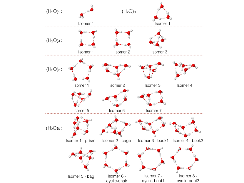
Figure 1: (H₂O)${}_{\text{n}}$ clusters used for the analysis of the many-body decomposition of the total interaction energies and harmonic frequencies.

All (H₂O)${}_{\text{n}}$ clusters, with n = 4$-$6, considered in the analysis of many-body contribution to the interaction energies are shown in Figure 1, while the errors associated with the individual terms are shown in Figure 2. As explained in Section II, the reference data were obtained with the CCSD(T)/CCSD(T)-F12b method in the CBS limit. Independently of the cluster size and geometry, MB-pol exhibits small errors, which are always within 0.5 kcal mol${{}^{\raisebox{0.60275pt}{$\scriptscriptstyle-1$}}}$ relative to the reference values, for all terms of the MBE of Eq. 1. The error in the total interaction energy increases with system size as the individual errors start to add up, most prevalently in ring-type configurations that consist of repeating dimer and trimer units. Due to extended hydrogen bonding and symmetry, the ring-type isomers also show larger higher-body contributions that can be non-negligible.Medders et al. (2015) The comparison between the reference and MB-pol interaction energies for the tetramer, pentamer, and hexamer isomers shown in Figure 3, indicates that the relative interaction energy order for the different isomers of each cluster is retained by MB-pol, with a maximum deviation in the computed interaction energies of 0.84 kcal mol${{}^{\raisebox{0.60275pt}{$\scriptscriptstyle-1$}}}$. In this analysis, the interaction energy is defined as the cluster energy minus the energy of the individual water molecules kept at the same geometry as in the cluster. The comparison in Figure 3 thus directly probes the actual interaction between water molecules without being affected by differences in the CCSD(T)/CCSD(T)-F12b and MB-pol representations of the monomer distortion energies.

Figure 2: Errors in the MB decomposition of the interaction energy, relative to the corresponding values calculated with the CCSD(T)/CCSD(T)-F12 method in the CBS limit, for the (H₂O)${}_{\text{n}}$ (n=4, 5, 6) clusters.

Scoring. To quantify the accuracy of MB-pol in describing many-body interactions, scores are assigned to each (H₂O)${}_{\text{n}}$ cluster based on the following three quantities. First, the maximum of the total unsigned error of the individual terms of the MBE, $\Delta\text{E}^{\text{MB}}_{\text{unsigned, max}}$, across all isomers of an $n$-mer,

$$\Delta\text{E}_{\text{unsigned, max}}^{\text{MB}}=\max_{i}\Big{[}\Big{(}\sum_{j}^{\text{NB}}\Big{|}\text{E}^{j}_{\text{MB-pol}}-\text{E}^{j}_{\text{Ref.}}\Big{|}\Big{)}_{\text{Isomer i}}\Big{]}.$$ (4)

Second, the maximum absolute error in the total interaction energy, $\Delta\text{E}_{\text{Int, max}}$, across all isomers of an $n$-mer,

$$\Delta\text{E}_{\text{Int, max}}=\max_{i}\Big{[}\Big{|}\Big{(}\sum_{j}^{\text{NB}}\text{E}^{j}_{\text{MB-pol}}-\text{E}^{j}_{\text{Ref.}}\Big{)}_{\text{Isomer i}}\Big{|}\Big{]}.$$ (5)

Third, the relative energy difference between the interaction energy of the prism and cage hexamer isomers,

$$\Delta\text{E}^{\text{Int}}_{\text{rel}}=\text{E}^{\text{Int}}_{\text{prism}}-\text{E}^{\text{Int}}_{\text{cage}}.$$ (6)

A small value for $\Delta\text{E}_{\text{Int, max}}$ with a larger error in $\Delta\text{E}^{\text{MB}}_{\text{unsigned, max}}$ would indicate that the MBE benefits from error compensation.

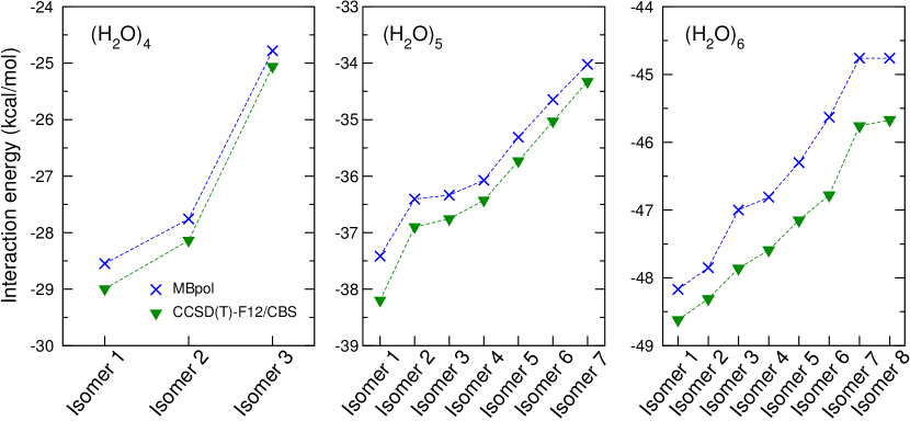
Figure 3: Interaction energies of all the low-lying isomers of the (H₂O)${}_{\text{n}}$ (n=4,5,6) clusters obtained with the MB-pol potential and the CCSD(T)/CCSD(T)-F12 method in the CBS limit.

For the first two criteria, 100 points are assigned if the magnitude of the error is less than 1 kcal mol${{}^{\raisebox{0.60275pt}{$\scriptscriptstyle-1$}}}$, which is commonly defined as chemical accuracy. 10 points are deducted successively for every 0.5 kcal mol${{}^{\raisebox{0.60275pt}{$\scriptscriptstyle-1$}}}$ increase in the error. For the third criterion, the reference value calculated using the CCSD(T)/CCSD(T)-F12/CBS method is $-$0.29 kcal mol${{}^{\raisebox{0.60275pt}{$\scriptscriptstyle-1$}}}$. A score of zero is assigned for the wrong sign while a score of 100 is assigned if the relative energy is within 0.1 kcal mol${{}^{\raisebox{0.60275pt}{$\scriptscriptstyle-1$}}}$ from the reference value. 10 points are deducted for every additional 0.1 kcal mol${{}^{\raisebox{0.60275pt}{$\scriptscriptstyle-1$}}}$ difference. The MB-pol values for the three criteria and associated scores are reported in Table 1, which demonstrates that MB-pol receives perfect scores in all three criteria for (H₂O)${}_{\text{n}}$ clusters with n = 4$-$6.

Table 1: Scores to assess the accuracy of MB-pol in describing many-body interaction energies in small water clusters. Energies are in kcal mol^-1. $\Delta\text{{E}}^{\text{MB}}_{\text{unsigned, max}}$ is the maximum total unsigned error, $\Delta{\text{E}}_{\text{Int, max}}$ is the maximum absolute total error in the many-body decomposition, $\Delta\text{{E}}^{\text{Int}}_{\text{rel}}$ is the difference between the interaction energy of the prism and cage hexamer isomers.

Cluster	$\Delta\text{E}^{\text{MB}}_{\text{unsigned, max}}$	Score	$\Delta\text{E}_{\text{Int, max}}$	Score	$\Delta\text{E}^{\text{Int}}_{\text{rel}}$	Score
(H2O)4	0.26	100	0.26	100	-	-
(H2O)5	0.72	100	0.72	100	-	-
(H2O)6	0.84	100	0.84	100	-0.32	100

III.1.2 Vibrational frequencies

The ability of MB-pol in predicting accurate vibrational frequencies is assessed through the analysis of harmonic frequencies calculated for small water clusters, from the water monomer to the hexamer. The comparisons are made with recently published benchmark data that are expected to closely approximate CCSD(T)/CBS values.Howard et al. (2014); Howard and Tschumper (2015)

The water clusters included in this analysis are all structures with lowest energy for n = 2 - 6, along with the cage, book1, and cyclic-chair (also referred to as ring) isomers of the hexamer (see Figure 1). For n = 3 - 5, the minimum energy structures correspond to cyclic structures in which each water molecule donates and accepts one hydrogen bond. In the water hexamer the lowest energy structure is the prism isomer, which is nearly isoenergetic with the cage isomer (see Section III.1.1), while the book1 and cyclic-chair isomers are higher in energy. Prism and cage are the predominant isomers at very low temperatures while the cage and cyclic-chair isomers appear at higher temperatures. Nauta and Miller (2000); Burnham et al. (2002); Elliott et al. (2008); Saykally and Wales (2012); Pérez et al. (2012); Wang et al. (2012); Babin and Paesani (2013)

Table 2: Average deviation (AD), average absolute deviation (AAD), and maximum absolute deviation (MAD) of MB-pol harmonic frequencies (in cm^-1) from benchmark data for the water monomer and (H₂O)${}_{\textrm{n}}$ clusters (n = 2$-$6). Scores are assigned based on the MAD value (see text).

	H2O	(H2O)2	(H2O)3	(H2O)4	(H2O)5	cyclic-chair	book1	cage	prism
AD	-1.3	-1.8	-1.7	-5.1	-6.0	-7.3	-5.4	-3.3	-2.8
AAD	1.3	4.4	4.7	11.6	15.6	16.5	12.7	8.9	7.8
MAD	2.2	12.0	16.5	31.4	46.2	49.4	38.6	23.0	24.1
Score	100	100	100	90	80	80	90	90	90

Table 2 reports the average deviation (AD), average absolute deviation (AAD), and the maximum absolute deviation (MAD) between the reference and the MB-pol harmonic frequencies calculated for the water monomer and each of the eight water clusters. The complete list of harmonic frequencies can be found in the Supplementary Material. In all cases, MB-pol accurately reproduces the reference data, with AAD and MAD values never exceeding 17 cm^-1 and 50 cm^-1, respectively. The MB-pol deviations from the reference data increase with increasing cluster size, in particular for cyclic structures, in which, as discussed in Section III.1.1, small errors in the MBE can add up for repeating units due to the inherent symmetry. As a result, the deviations for the hexamer book1, cage, and prism isomers are smaller than for the cyclic-chair isomer. On average, the MB-pol harmonic frequencies are slightly redshifted as compared to the reference data. This redshift is mostly due to the low-frequency intermonomer and bending modes, while the OH stretch frequencies are slightly blueshifted (see list of frequencies in the Supporting Information). Both red and blue shifts associated, respectively, with the bending and stretching vibrations can be explained by considering that MB-pol does not allow water autoionization, and, consequently, underestimates the ionic character, and thus the strength, of the hydrogen bonds. Importantly, it has been shown that MB-pol provides a consistent representation of the vibrational structure of water independently of the system size, correctly predicting infrared,Medders and Paesani (2015a) Raman,Medders and Paesani (2015a) sum-frequency generation,Medders and Paesani (2016) and two-dimensional infraredStraight and Paesani (2016) spectra of liquid water at ambient conditions.

Scoring. To quantify the accuracy with which MB-pol reproduces the reference harmonic frequencies, a score for each cluster is assigned based on the corresponding MAD value. A score of 100 is assigned if the MAD is below the threshold value of 20 cm${{}^{\raisebox{0.60275pt}{$\scriptscriptstyle-1$}}}$, and 10 points are then deducted for each additional increment of 20 cm${{}^{\raisebox{0.60275pt}{$\scriptscriptstyle-1$}}}$. The MB-pol scores are reported in Table 2.

III.2 Thermodynamic properties of liquid water

The accuracy of MB-pol in reproducing the properties of liquid water is assessed through comparisons with the corresponding experimental data as a function of temperature. As discussed in detail in Section II, all MB-pol properties were calculated from classical MD simulations. The role played by NQE (e.g., zero-point energy and tunneling) will be discussed in a forthcoming publication. A summary of several thermodynamic properties of liquid water computed with MB-pol at atmospheric pressure (P = 1 atm) along with the corresponding experimental values is reported in the Supplementary Material (Tables XL and XLI).

III.2.1 Density

The temperature dependence of the density of liquid water at 1 atm calculated from classical MD simulations with MB-pol is shown in Figure 4. The experimental data are taken from Refs. 99 and 100. At high temperature, the MB-pol results are in excellent agreement with the corresponding experimental values. As the temperature decreases, the difference between MB-pol and experiment increases nearly linearly. The maximum and average absolute deviations from the reference values are 0.042 and 0.013 g cm^-3, respectively. The temperature of maximum density, obtained by calculating the analytical derivative of a fifth-order polynomial interpolating the simulation results, is located at 263 K, which is 14 K lower than experiment.Speedy (1987); W. Wagner and A. Pruß (2002) The systematic deviation between the MB-pol and the experimental values as the temperature decreases can be attributed, at least in part, to the neglect of NQE in the simulations, which, as expected, become increasingly important at lower temperature.Ceriotti et al. (2016) In this context, at 298 K, the density predicted by classical MD simulations with MB-pol is 1.007 g cm^-3 compared to the experimental value of 0.997 g cm^-3. Using path-integral molecular dynamics (PIMD) simulations, which explicitly include NQE, it was shown that the density of water predicted by MB-pol at the same temperature decreases by 0.6%,Medders et al. (2014) in excellent agreement with the experimental value.

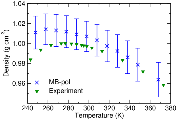
Figure 4: Densities of liquid water at atmospheric pressure from MB-pol. Experimental data are taken from Refs.99 and 100.

III.2.2 Enthalpy of vaporization

The enthalpy of vaporization, $\Delta H_{vap}$, is one of the properties usually included in the fitting procedures to parameterize empirical water potentials Abascal and Vega (2005); Horn et al. (2004) and is defined as

$$\Delta H_{vap}=H_{gas}-H_{liquid}=U_{gas}-U_{liquid}+P(V_{gas}-V_{liquid}),$$ (7)

where $H$, $U$, and $V$ are the enthalpy, internal energy, and volume, respectively, and the subscripts denote that the molecules are in either the gas or liquid state. Since, at low pressure, the gas can be considered ideal, the contribution to $U_{gas}$ due to interactions between water molecules can be neglected and $\Delta H_{vap}$ can then be rewritten (for 1 mol of water) as

$$\Delta H_{vap}=U_{gas}-U_{liquid}-PV_{liquid}+RT,$$ (8)

where $U_{gas}$ contains the average kinetic (i.e., 3/2 RT) and potential (i.e., intramolecular distortion) energies of the gas molecules. At each temperature, the average potential energy was calculated from a 2 ns long classical MD simulation of a single water molecule. It should be noted that, unlike point charge models, $\Delta H_{vap}$ calculated with MB-pol implicitly includes the self-polarization correction,Abascal and Vega (2005); Horn et al. (2004) since MB-pol correctly describes the change in dipole moment from the gas to the condensed phase.

Figure 5 shows that $\Delta H_{vap}$ calculated from classical MD simulations with MB-pol is systematically larger than the corresponding experimental values, with an average absolute deviation of 0.41 kcal mol${{}^{\raisebox{0.60275pt}{$\scriptscriptstyle-1$}}}$. As for the density, the deviation from experiment increases as the temperature decreases, which can be attributed to the neglect of NQE in the simulations. At 298 K, $\Delta H_{vap}$ predicted by MB-pol is 10.93 kcal mol${{}^{\raisebox{0.60275pt}{$\scriptscriptstyle-1$}}}$, 0.42 kcal mol${{}^{\raisebox{0.60275pt}{$\scriptscriptstyle-1$}}}$ larger than the experimental value. Guillot and Guissani suggested that $\Delta H_{vap}$ for hypothetical “classical water” at 298.15 K should be 11.0 kcal mol${{}^{\raisebox{0.60275pt}{$\scriptscriptstyle-1$}}}$,Guillot and Guissani (2001) which is in excellent agreement with the value obtained from classical MD simulations with MB-pol.

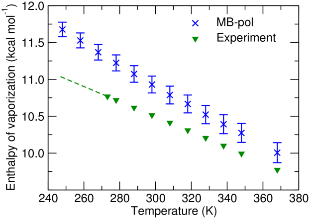
Figure 5: Enthalpy of vaporization of liquid water at atmospheric pressure calculated using MB-pol. Experimental data is provided for comparison.W. Wagner and A. Pruß (2002) The dashed line corresponds to the extrapolated data.

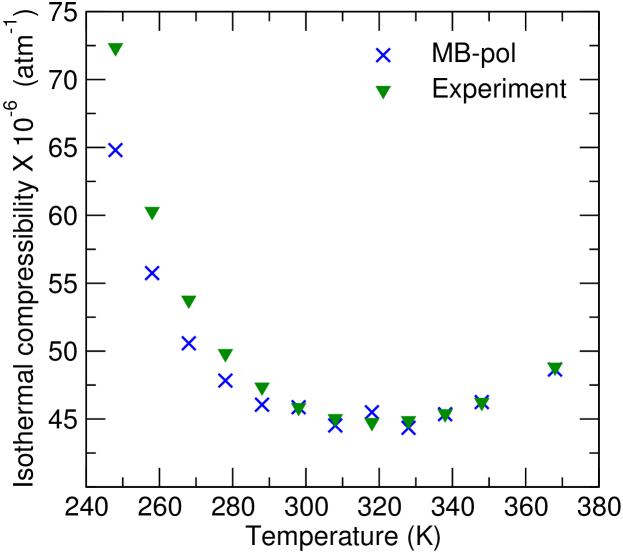
Figure 6: Isothermal compressibility of liquid water at atmospheric pressure calculated using MB-pol. Experimental data are taken from Ref.103.

III.2.3 Isothermal compressibility

The isothermal compressibility, $\kappa_{T}$, is defined as

$$\kappa_{T}=-{\frac{1}{V}}\left({\frac{\partial V}{\partial P}}\right)_{T},$$ (9)

where $V$ and $P$ are the volume and the pressure of liquid water at a given temperature $T$, respectively. To solve Eq. 9, classical MD simulations with MB-pol were carried out at each temperature for seven pressure values (-1.5, -1.0, -0.5, 0.001, 0.5, 1.0, 1.5 katm), which were used to determine the corresponding average volumes. $\kappa_{T}$ was then calculated from the derivative of a third-order polynomial that was used to fit the volumes as a function of pressure at each temperature. As shown in Figure 6, the MB-pol values are in good agreement with the corresponding experimental data,Kell (1975) correctly predicting a minimum between 310 and 330 K. The average and maximum absolute deviations from experiment in the temperature range between the freezing and the boiling point are 0.5$\times$10^-6 and 1.8$\times$10^-6 atm${{}^{\raisebox{0.60275pt}{$\scriptscriptstyle-1$}}}$, respectively. As expected, the deviations from the experimental data become more pronounced at low temperature due to the neglect of NQE in classical MD simulations.

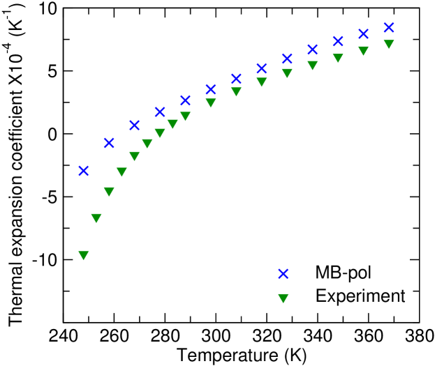
Figure 7: Thermal expansion coefficient of liquid water at atmospheric pressure. Experimental data are taken from Ref.103.

III.2.4 Thermal expansion coefficient

The thermal expansion coefficient, $\alpha_{P}$, is defined as

$$\alpha_{P}=-{\frac{1}{V}}\left({\frac{\partial V}{\partial T}}\right)_{P}=-{\frac{1}{\rho}}\left({\frac{\partial\rho}{\partial T}}\right)_{P}.$$ (10)

where $V$, $T$, and $\rho$ are the volume, the temperature, and the density of liquid water at a given pressure $P$, respectively. From Eq. 10, it is evident that any water model that accurately predicts the temperature dependence of the density is also capable of correctly reproducing the variation of $\alpha_{P}$. The MB-pol values of $\alpha_{P}$, shown in Figure 7 along with the corresponding experimental data,Kell (1975) were determined numerically by solving Eq. 10 using the density values reported in Figure 4. Similar to $\rho$, $\alpha_{P}$ derived from classical MD simulations with MB-pol is in close agreement with experiment above the freezing point, with average and maximum absolute deviations of 1.3$\times$10^-4 and 1.7$\times$10^-4 K${{}^{\raisebox{0.60275pt}{$\scriptscriptstyle-1$}}}$, respectively. At the classical level, MB-pol predicts $\alpha_{P}$ to be zero at 263 K, in line with the density maximum reported in Section III.2.1 (experimentally, $\alpha_{P}=0$ at 277 K). Again, NQE appear to be important to quantitatively reproduce the variation $\alpha_{P}$ at low temperature, as already found in previous sections for other thermodynamic properties of liquid water.

III.2.5 Isobaric heat capacity

The isobaric heat capacity, c_P, is defined as

$$c_{P}=\left({\frac{\partial H}{\partial T}}\right)_{P},$$ (11)

where $H$ and $T$ are the enthalpy and the temperature of liquid water at a given pressure $P$, respectively. It should be noted that, unlike other thermodynamic properties, $c_{P}$ is significantly affected by NQE even at room temperature.Shiga and Shinoda (2005); Vega et al. (2010) Using Eq. 11, $c_{P}$ was calculated as the temperature derivative of a fifth-order polynomial interpolating the values of $H$ obtained at different temperatures from classical MD simulations carried out in the NPT ensemble. Consistent with previous studies, the classical MB-pol results shown in Figure 8 are larger than the corresponding experimental data W. Wagner and A. Pruß (2002); Archer et al. (2000) at all temperatures. Experimentally, it is known that the difference between the heat capacity of liquid H₂O and D₂O increases as the temperature decreases.Angell et al. (1982) For example, the heat capacity of H₂O and D₂O at 250 K are 19.07 and 23.93 cal mol${{}^{\raisebox{0.60275pt}{$\scriptscriptstyle-1$}}}$ K${{}^{\raisebox{0.60275pt}{$\scriptscriptstyle-1$}}}$, respectively.W. Wagner and A. Pruß (2002); Archer et al. (2000); Angell et al. (1982) The corresponding value obtained from classical MD simulations with MB-pol is 29.25 cal mol${{}^{\raisebox{0.60275pt}{$\scriptscriptstyle-1$}}}$ K${{}^{\raisebox{0.60275pt}{$\scriptscriptstyle-1$}}}$, reinforcing the notion that explicit inclusion of NQE in simulations with MB-pol is required for quantitative, and physically correct, calculations of $c_{P}$ at all temperatures. Levitt et al. estimated that 6 cal mol${{}^{\raisebox{0.60275pt}{$\scriptscriptstyle-1$}}}$ K${{}^{\raisebox{0.60275pt}{$\scriptscriptstyle-1$}}}$  must be subtracted from the classical value of the heat capacity at constant volume, $c_{V}$, to account for NQE at 298.15 K. Levitt et al. (1997) Assuming that the same correction can be applied to $c_{P}$, the quantum-corrected MB-pol result at 298 K becomes 21.85 cal mol${{}^{\raisebox{0.60275pt}{$\scriptscriptstyle-1$}}}$ K${{}^{\raisebox{0.60275pt}{$\scriptscriptstyle-1$}}}$, in closer agreement with the experimental value.

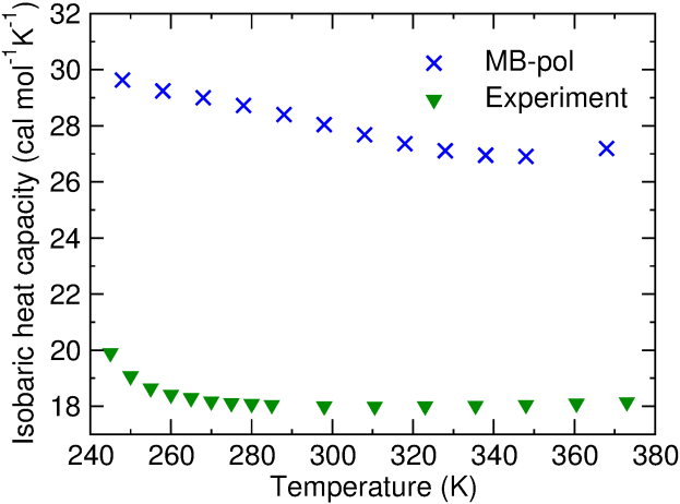
Figure 8: Isobaric heat capacity of liquid water at atmospheric pressure. Experimental data are taken from Refs.100 and 106.

III.2.6 Surface tension

The surface tension, $\gamma$, can be calculated from MD simulations asRowlinson and Widom (1982)

$$\gamma=\int_{z_{\alpha}}^{z_{\beta}}\left[P_{N}(z)-P_{T}(z)\right]dz,$$ (12)

where the z-direction is defined along the normal vector to the surface, $\alpha$ and $\beta$ refer to the liquid and the gas phase, respectively, and N and T denote the normal and tangential components of the pressure tensor, respectively. Considering the slab geometry defined in Section II, Eq. 12 reduces to

$$\gamma=\frac{1}{2}L_{z}\left<P_{zz}-\frac{1}{2}\left(P_{xx}+P_{yy}\right)\right>,$$ (13)

where $P_{xx}$, $P_{yy}$, and $P_{zz}$ are the diagonal elements of the pressure tensor, $L_{z}$ is the length of the simulation box in the z-direction, and the angular brackets denote an ensemble average. The comparison between the experimentalVargaftik et al. (1983); Vinš et al. (2015) and MB-pol values of the surface tension is shown in Figure 9. Overall, the MB-pol results are in good agreement with experiment over the entire temperature range considered in this study, correctly reproducing (within statistical uncertainty) the linear increase of $\gamma$ as the temperature decreases. At 298 K, the surface tension obtained from classical MD simulations with MB-pol is $66.8\pm 3.55$ mJ m^-2 compared to the experimental value of 71.97 mJ m^-2.Vargaftik et al. (1983) Contrary to other thermodynamic properties, the differences between the experimental and MB-pol values of the surface tension remain effectively constant as a function of temperature, suggesting that $\gamma$ is less sensitive to NQE.

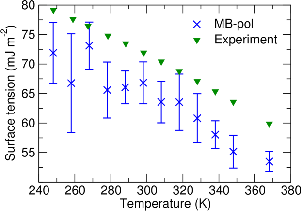
Figure 9: Surface tension of liquid water at atmospheric pressure. Experimental data are taken from Refs.110 and 111.

III.2.7 Static dielectric constant

The static dielectric constant, $\epsilon$, is defined as

$$\epsilon=1+\frac{4\pi}{3Vk_{B}\left<T\right>}\left(\left<\mathbf{M}^{2}\right>-\left<\mathbf{M}\right>^{2}\right),$$ (14)

where M is the total dipole moment of the simulation box, $k_{B}$ is Boltzmann’s constant, $V$ and $T$ are the volume and the temperature, respectively, and the angular brackets denote an ensemble average. The temperature dependence of the dielectric constant calculated from classical MD simulations with MB-pol is compared in Figure 10 with the corresponding experimental data.Fernández et al. (1997) $\epsilon$ calculated from the MB-pol simulations is in good agreement with experiment over the entire temperature range considered in this study. At 298 K, the value of $\epsilon$ obtained from the MB-pol simulations is 68.4 which is $\sim$13% smaller than the experimental value of 78.5. These differences may be related, at least in part, to (small) differences in the liquid structure due to the neglect of NQE,Medders et al. (2014) which, in turn, may affect the dipole moments of the water molecules.

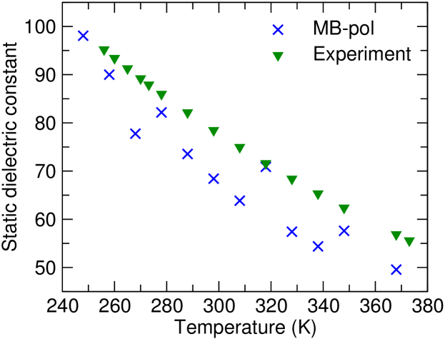
Figure 10: Static dielectric constant of liquid water at atmospheric pressure. Experimental data are taken from Ref.112.

III.2.8 Self-diffusion coefficient

The self-diffusion coefficient, D, of liquid water can be computed from the velocity autocorrelation function as

$$D=\frac{1}{3}\int_{0}^{\infty}\left<v_{i}(t)v_{i}(0)\right>dt,$$ (15)

where $v_{i}$ is the velocity of the center of mass of $i^{th}$ water molecule and the brackets indicate an ensemble average in the microcanonical (NVE) ensemble. The MB-pol results are compared in Figure 11 with the corresponding experimental values. Gillen et al. (1972); Holz et al. (2000); Easteal et al. (1989); Mills (1973) At 298 K, classical MD simulations with MB-pol predict $D$ to be $0.23\pm 0.02$ Ų ps${{}^{\raisebox{0.60275pt}{$\scriptscriptstyle-1$}}}$ in agreement with the experimental value of 0.229 Ų ps${{}^{\raisebox{0.60275pt}{$\scriptscriptstyle-1$}}}$. It should be mentioned that an incorrect value for the classical MB-pol diffusion coefficient at room temperature was previously reported by some of us in Ref. 55. The similarity between the present classical value and the corresponding quantum value obtained in Ref. 55 from centroid molecular dynamics simulations suggests the presence of competing NQE in the water diffusion as originally suggested in Ref. 20.

Since it was shown that the calculation of the self-diffusion coefficient from MD simulations is particularly sensitive to the system size,Yeh and Hummer (2004) additional NVE simulations were carried out for a system containing 512 molecules. For this larger system, $D=0.24\pm 0.02$ Ų ps${{}^{\raisebox{0.60275pt}{$\scriptscriptstyle-1$}}}$ at room temperature. The self-diffusion coefficient in the limit of an infinite system size can be calculated asDünweg and Kremer (1993); Yeh and Hummer (2004)

$$D(\infty)=D(L)+\frac{\xi k_{B}T}{6\pi\eta L},$$ (16)

where $k_{B}$ is Boltzmann’s constant, $T$ is the temperature, $\eta$ is the viscosity, and $\xi$ is a constant that depends on the shape of the simulation box (for cubic, $\xi=2.837297$). Plugging the values obtained for 256 and 512 water molecules into Eq. 16, and using the experimental value for $\eta$, $D(\infty)=0.280\pm 0.040$ Ų ps${{}^{\raisebox{0.60275pt}{$\scriptscriptstyle-1$}}}$ at 298 K.

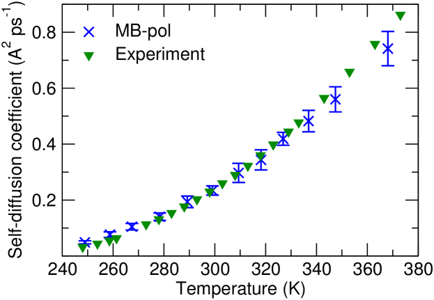
Figure 11: Self-diffusion coefficient of liquid water at atmospheric pressure. Experimental data are taken from Refs.113; 114; 115; 116.

Table 3: Scores calculated for MB-pol at 248, 298, and 360 K based on threshold criteria (x_tol) set for each property. See text for more details. Interpolated data are used at 360 K. $\rho$ is the density; c_P is the heat capacity; $\Delta H_{vap}$ is the enthalpy of vaporization; $\kappa_{T}$ is the isothermal compressibility; $\epsilon$ is the dielectric constant; D is the self-diffusion coefficient; $\gamma$ is the surface tension.

Property	xtol (%)	Scores
		248 K	298 K	360 K
$\rho$	0.5	60	80	100
$\Delta H_{vap}$	2.5	80	90	100
$\kappa_{T}$	5	80	100	100
$\alpha_{P}$	0.5	90	100	100
cP	5	90	100	100
$\gamma$	2.5	70	80	60
$\epsilon$	5	100	80	80
$D$	5	0	100	90
Average		71	91	91

Scoring. As in Section III.1, scores are assigned to each property of liquid water calculated with MB-pol. Following the procedure described in Refs. 4, 17, and 9, the relative error ($\delta x$) associated with each property was used to define the corresponding score as

$$\text{score}=\mathrm{max}\left\{100-\mathrm{int}(\delta x/x_{tol})\times 10,0\right\},$$ (17)

where $\delta x=|x_{sim}-x_{exp}|/|x_{exp}|$ and $x_{tol}$ is the threshold value. The score is 100 if the $\delta x$ value is between 0 and $x_{tol}$. The score is thus reduced by 10% for each successive increment by x_tol. A score of 100 indicates perfect agreement with experiment while a score of 0 indicates poor performance. The $x_{tol}$ value for each property was taken from Ref. 4, except for $\alpha_{P}$ that was not included in that study. The scores were calculated at three different temperatures. The first temperature selected to assess the performance of MB-pol is 248 K since the maximum absolute deviations for all properties calculated from classical MD simulations with MB-pol are observed at this temperature. As mentioned above, since NQE are not included in the present MB-pol simulations, it is not surprising that the computed values deviate significantly from experiment, especially at low temperatures. The performance of MB-pol is also assessed at room temperature (298 K) and at higher temperature (360 K). Polynomial fits were used to obtain the values of all properties at 360 K. Table 3 shows the scores obtained from classical MD simulations with MB-pol for all properties discussed in the previous sections. The average scores of MB-pol are 71, 91, and 91 at 248, 298, and 360 K, respectively.

III.3 Structural properties of liquid water

Figure 12 shows the oxygen-oxygen (OO) radial distribution function (RDF) calculated with MB-pol at several temperatures along with the corresponding experimental curves derived from the most recent X-ray diffraction measurements.Skinner et al. (2014, 2013) The MB-pol RDFs are in good agreement with the experimental data at all temperatures, although they slightly overestimate the height of the first peak. As discussed in previous studies, this difference, which increases with decreasing temperature, can be attributed to the the neglect of NQE and lead to more structural order in the classical liquid than is experimentally observed. It has been shown that, while the position of the first peak moves to larger r_OO linearly with increasing temperature, the shift in the position of the second peak deviates from a linear dependence on r${}_{\textrm{OO}}$ above $\sim$320 K.Skinner et al. (2014) This trend is correctly captured by classical NPT simulations with MB-pol, which reproduce the experimental data nearly quantitatively (Figure 13). The numerical comparison between MB-pol and experimental OO RDFs is based on the position of the 1^st (r₁) and 2^nd (r₂) peaks, and the height of the 1^st peak (g(r₁)) reported in Table 4. Altogether, these quantities are used to assess the accuracy of MB-pol at 268, 278, and 308 K, through comparisons with the corresponding experimental values.Skinner et al. (2014, 2013)

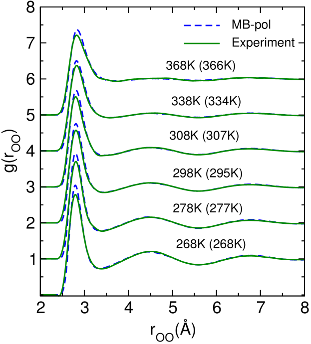
Figure 12: Temperature dependence of the oxygen-oxygen RDF of liquid water predicted by classical NPT simulations with MB-pol compared with the corresponding results derived from X-ray diffraction measurements.120; 119. The temperatures at which the experimental measurements were performed are given in parenthesis.

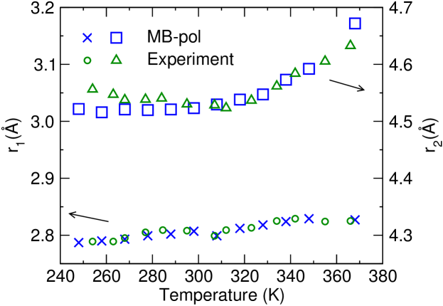
Figure 13: Temperature dependence of the positions of the first and second peaks of the oxygen-oxygen RDF of liquid water predicted by classical NPT simulations with MB-pol compared with the corresponding experimental data.Skinner et al. (2013, 2014)

Scoring. In addition to the numerical comparison, a score was assigned to each of the three quantities using Eq. 17 with tolerance values of 0.1%, 0.5% and 5.0% respectively for the r₁, r₂ and g(r₁). The average MB-pol scores obtained for the three quantities at at 268, 278, and 308 K are listed in Table 4. The agreement between the calculated and experimental data is excellent at all temperatures, which provides further evidence for the accuracy and transferability of MB-pol.

Table 4: Positions of the first (r₁) and second (r₂) peaks (in Å), and first peak height (g(r₁)) of the oxygen-oxygen RDF of liquid water predicted by classical NPT simulations with MB-pol at three different temperatures compared with the corresponding experimental data.Skinner et al. (2013, 2014) The temperatures at which the experimental measurements were performed are given in parenthesis.See text for details.

	268 K		278 (277) K		308 (307) K
	MB-pol	Experiment	MB-pol	Experiment	MB-pol	Experiment
r1	2.796	2.798	2.806	2.797	2.818	2.806
r2	4.488	4.509	4.490	4.516	4.510	4.520
g(r1)	3.044	2.801	2.936	2.723	2.678	2.484
Average score	90	-	93	-	93	-

III.4 Ice phases

III.4.1 Melting point of hexagonal ice

The melting point (T${}_{\textrm{m}}$) of hexagonal ice (I${}_{\textrm{h}}$) at the pressure of 1 atm was calculated from classical MD simulations carried out in the NPT ensemble to characterize the ice/water coexistence as a function of temperature. This approach, originally proposed in Refs.121; 122; 123, has been used to determine the melting point of several water models. Karim and Haymet (1988); Karim et al. (1990); Bryk and Haymet (2002, 2004); Wang et al. (2005); Fernández et al. (2006) The water and ice I${}_{\textrm{h}}$ regions of the coexistence system, each containing 360 water molecules, were equilibrated independently at 300 and 100 K, respectively. The two regions were then combined into a single rectangular box of 720 water molecules (dimensions 22.57 $\times$ 23.46 $\times$ 44.24 ų) with the basal (0001) plane of ice I${}_{\textrm{h}}$ in contact with the liquid phase. Direct coexistence simulations were then carried out in the NPT ensemble at different temperatures, during which the enthalpy of the combined system was monitored. The melting point was determined as the temperature at which the enthalpy of the combined system remained constant throughout the entire trajectory. The classical melting point of MB-pol is found at 263.5 $\pm$ 1.5 K. The calculated T${}_{\textrm{m}}$ is $\sim$9 K lower than the experimental value and in good agreement with the classical MB-pol estimate of 263 K for the temperature of maximum density (see Section III.2.1).

III.4.2 Lattice energies and densities of ice phases

Table 5 lists the lattice energies of different ice phases predicted by MB-pol in comparison with the corresponding experimental estimates. The MB-pol values were obtained from single point calculations carried out for the experimental crystal structures taken from Ref. 88. In all cases, the MB-pol results are in excellent agreement with the experimental values. The maximum deviation of $\sim$2% is found for ice VIII, a high density phase. A detailed analysis of the lattice energies in terms of many-body contributions will be reported in a forthcoming publication.

Table 5: Melting point (in K) of hexagonal ice along with lattice energies (in meV) and densities (in g cm^-3) of several ice phases calculated using MB-pol. Scores assigned to each computed quantity are also listed. See text for details.

Ice	Melting point				Lattice energy						Density
	MB-pol	Exp.	Score		MB-pol	Exp.	Score		T(K)	P(bar)	MB-pol	Exp.	Score
I${}_{\textrm{h}}$	263.5	273	90		-611	-610	100		250	0	0.921	0.920	100
II	-	-	-		-603	-609	100		123	0	1.198	1.190	100
VIII	-	-	-		-590	-577	80		263	24000	1.658	1.611	80
IX	-	-	-		-601	-606	100		165	2800	1.208	1.194	90
XIII	-	-	-		-595	-	-		80	1	1.281	1.251	80
XIV	-	-	-		-592	-	-		80	1	1.312	1.294	90
XV	-	-	-		-587	-	-		80	0	1.364	1.326	80
Average score			90				95						89

The densities of several ice phases calculated from classical NPT simulations with MB-pol at different temperatures and pressures are compared in Table 5 with the corresponding experimental data. Röttger et al. (1994); Fortes et al. (2005); Kuhs et al. (1984); Londono et al. (1993); Petrenko and Whitworth (1999, 1999); Salzmann et al. (2009) Excellent agreement is found between the theoretical predictions and the experimental values, with the largest relative error being less than 3% for ice VIII. It should be noted that the classical NPT simulations with MB-pol slightly overestimates the densities of all ice phases, which again indicates that explicit inclusion of NQE is necessary for more quantitative comparisons with the experimental data. In this context, it was demonstrated that quantum simulations are indeed strictly required to correctly compare the theoretical results with the experimental data at temperatures below 100 K.McBride et al. (2009) Similar to liquid water,Medders et al. (2014) NQE are expected to lower the density and, therefore, improve the agreement with experiment, especially for the ice phases (XIII, XIV, and XV) that are stable at lower temperature.

Scoring. Adopting the same scoring scheme used for the liquid properties (Eq. 17), scores were assigned to both lattice energies and densities calculated with MB-pol for the different ice phases considered in this analysis, setting the tolerance value to 1% for both properties. For the melting point, it is set to 2.5% which is the same as used in Ref. 4. As shown in Table 5, the average scores received by MB-pol are 95 and 89 for ice lattice energies and densities, respectively, which, combined with the analyses reported in the previous sections, demonstrate that MB-pol consistently achieves high accuracy in predicting the properties of water from clusters to the liquid phase and ice.

IV Conclusions

In this study, the accuracy of the MB-pol many-body potential is assessed from extensive analysis of the energetics as well as of spectroscopic, structural, thermodynamic, and dynamical properties of water from the gas to the condensed phase.

The analysis of gas-phase properties shows that both individual many-body contributions to the interaction energies and harmonic frequencies calculated for water clusters up to the hexamer with MB-pol are in excellent agreement with reference data obtained at the coupled cluster level of theory. The largest deviations are observed for cyclic clusters due to the accumulation of errors associated with repeating, symmetry-equivalent two-body and three-body units in the MB-pol representation of the underlying Born-Oppenheimer PES.

For the liquid phase, classical MD simulations carried out with MB-pol correctly reproduce the temperature dependence of all structural, thermodynamic, and dynamical properties analyzed in this study. The deviations from the experimental values increase as the temperature decreases. Since MB-pol was derived entirely from electronic structure data and thus represents the water Born-Oppenheimer PES, the differences between results obtained from classical MD simulations with MB-pol and experimental data are expected and confirm that nuclear quantum effects must be explicitly taken into account in the simulations with MB-pol for a quantitative (and rigorous) description of the molecular properties of liquid water. Finally, the melting point of hexagonal ice as well as both lattice energies and densities calculated with MB-pol for several ice phases are found in good agreement with the corresponding experimental data, which provides further evidence for the transferability of MB-pol.

Besides demonstrating the high and, in many respects, unprecedented accuracy with which MB-pol predicts the properties of water across different phases, this study also provides a series of rigorous tests that should be used to assess the ability of both empirical and ab initio water models “to get the right answers for the right reasons”,Paesani (2016) which is the fundamental prerequisite for a physically correct understanding of the behavior of water at the molecular level.

V Supplementary Material

List of Additional data related to the analysis of many-body interactions and vibrational frequencies of water clusters along with the corresponding molecular coordinates. Tables with numerical values for all water properties shown in Figures 4 - 11.

VI Acknowledgements

This research was supported by the National Science Foundation through Grant CHE-1453204. This work was performed in part under the auspices of the US DOE by LLNL under Contract DE-AC52-07NA27344. This research used resources of the Argonne Leadership Computing Facility, which is a DOE Office of Science User Facility supported under Contract DE-AC02-06CH11357, as well as the Extreme Science and Engineering Discovery Environment (XSEDE), which is supported by the National Science Foundation (Grant ACI-1053575). S.S. acknowledges the University of California, San Diego for financial support through the Frontiers of Innovation Scholars Program (FISP).

The submitted manuscript has been created by UChicago Argonne, LLC, Operator of Argonne National Laboratory (“Argonne”). Argonne, a U.S. Department of Energy Office of Science laboratory, is operated under Contract No. DE-AC02-06CH11357. The U.S. Government retains for itself, and others acting on its behalf, a paid-up nonexclusive, irrevocable worldwide license in said article to reproduce, prepare derivative works, distribute copies to the public, and perform publicly and display publicly, by or on behalf of the Government.

References

- Cisneros et al. (2016) G. A. Cisneros, K. T. Wikfeldt, L. Ojamäe, J. Lu, Y. Xu, H. Torabifard, A. P. Bartók, G. Csányi, V. Molinero, and F. Paesani, Chem. Rev. 116, 7501 (2016).
- Bukowski et al. (2007) R. Bukowski, K. Szalewicz, G. C. Groenenboom, and A. van der Avoird, Science 315, 1249 (2007).
- Cencek et al. (2008) W. Cencek, K. Szalewicz, C. Leforestier, R. van Harrevelt, and A. van der Avoird, Phys. Chem. Chem. Phys. 10, 4716 (2008).
- Vega and Abascal (2011) C. Vega and J. L. F. Abascal, Phys. Chem. Chem. Phys. 13, 19663 (2011).
- Marx and Hutter (2009) D. Marx and J. Hutter, Ab initio molecular dynamics: Basic theory and advanced methods (Cambridge University Press, 2009).
- Car and Parrinello (1985) R. Car and M. Parrinello, Phys. Rev. Lett. 55, 2471 (1985).
- Schlegel et al. (2002) H. B. Schlegel, S. S. Iyengar, X. Li, J. M. Millam, G. A. Voth, G. E. Scuseria, and M. J. Frisch, J. Chem. Phys. 117, 8694 (2002).
- Payne et al. (1992) M. C. Payne, M. P. Teter, D. C. Allan, T. A. Arias, and J. D. Joannopoulos, Rev. Mod. Phys. 64, 1045 (1992).
- Gillan et al. (2016) M. J. Gillan, D. Alfè, and A. Michaelides, J. Chem. Phys. 144, 130901 (2016).
- Guillot (2002) B. Guillot, J. Mol. Liq. 101, 219 (2002).
- Shvab and Sadus (2016) I. Shvab and R. J. Sadus, Fluid Phase Equilib. 407, 7 (2016).
- Abascal and Vega (2005) J. L. Abascal and C. Vega, J. Chem. Phys. 123, 234505 (2005).
- Horn et al. (2004) H. W. Horn, W. C. Swope, J. W. Pitera, J. D. Madura, T. J. Dick, G. L. Hura, and T. Head-Gordon, J. Chem. Phys. 120, 9665 (2004).
- Jorgensen et al. (1983) W. L. Jorgensen, J. Chandrasekhar, J. D. Madura, R. W. Impey, and M. L. Klein, J. Chem. Phys. 79, 926 (1983).
- Mahoney and Jorgensen (2000) M. W. Mahoney and W. L. Jorgensen, J. Chem. Phys. 112, 8910 (2000).
- Berendsen et al. (1987) H. J. C. Berendsen, J. R. Grigera, and T. P. Straatsma, J. Phys. Chem. 91, 6269 (1987).
- Vega et al. (2009) C. Vega, J. L. F. Abascal, M. M. Conde, and J. L. Aragones, Faraday Discuss. 141, 251 (2009).
- Reimers et al. (1982) J. Reimers, R. Watts, and M. Klein, Chem. Phys. 64, 95 (1982).
- Berendsen et al. (1981) H. J. C. Berendsen, J. P. M. Postma, W. F. van Gunsteren, and J. Hermans, in Intermolecular Forces: Proceedings of the Fourteenth Jerusalem Symposium on Quantum Chemistry and Biochemistry Held in Jerusalem, Israel, April 13–16, 1981, edited by B. Pullman (Springer Netherlands, Dordrecht, 1981), pp. 331–342.
- Habershon et al. (2009) S. Habershon, T. E. Markland, and D. E. Manolopoulos, J. Chem. Phys. 131, 024501 (2009).
- Paesani et al. (2006) F. Paesani, W. Zhang, D. A. Case, T. E. Cheatham, and G. A. Voth, J. Chem. Phys. 125, 184507 (2006).
- Kumar and Skinner (2008) R. Kumar and J. L. Skinner, The Journal of Physical Chemistry B 112, 8311 (2008).
- Tainter et al. (2011) C. J. Tainter, P. A. Pieniazek, Y.-S. Lin, and J. L. Skinner, J. Chem. Phys. 134, 184501 (2011).
- Tainter et al. (2015) C. J. Tainter, L. Shi, and J. L. Skinner, Journal of Chemical Theory and Computation 11, 2268 (2015).
- Kiss and Baranyai (2013) P. T. Kiss and A. Baranyai, J. Chem. Phys. 138, 204507 (2013).
- Lamoureux et al. (2003) G. Lamoureux, A. D. MacKerell, and B. Roux, J. Chem. Phys. 119, 5185 (2003).
- Lamoureux et al. (2006) G. Lamoureux, E. Harder, I. V. Vorobyov, B. Roux, and A. D. M. Jr., Chem. Phys. Lett. 418, 245 (2006).
- Yu et al. (2013) W. Yu, P. E. M. Lopes, B. Roux, and A. D. MacKerell, J. Chem. Phys. 138, 034508 (2013).
- Yu et al. (2003) H. Yu, T. Hansson, and W. F. van Gunsteren, J. Chem. Phys. 118, 221 (2003).
- Yu and van Gunsteren (2004) H. Yu and W. F. van Gunsteren, J. Chem. Phys. 121, 9549 (2004).
- Fanourgakis and Xantheas (2006) G. S. Fanourgakis and S. S. Xantheas, J. Phys. Chem. A 110, 4100 (2006).
- Fanourgakis and Xantheas (2008) G. S. Fanourgakis and S. S. Xantheas, J. Chem. Phys. 128, 074506 (2008).
- Burnham et al. (2008) C. J. Burnham, D. J. Anick, P. K. Mankoo, and G. F. Reiter, J. Chem. Phys. 128, 154519 (2008).
- Ren and Ponder (2003) P. Ren and J. W. Ponder, J. Phys. Chem. B 107, 5933 (2003).
- Ponder et al. (2010) J. W. Ponder, C. Wu, P. Ren, V. S. Pande, J. D. Chodera, M. J. Schnieders, I. Haque, D. L. Mobley, D. S. Lambrecht, J. Robert A. DiStasio, et al., J. Phys. Chem. B 114, 2549 (2010).
- Wang et al. (2013) L.-P. Wang, T. Head-Gordon, J. W. Ponder, P. Ren, J. D. Chodera, P. K. Eastman, T. J. Martinez, and V. S. Pande, J. Phys. Chem. B 117, 9956 (2013).
- Laury et al. (2015) M. L. Laury, L.-P. Wang, V. S. Pande, T. Head-Gordon, and J. W. Ponder, J. Phys. Chem. B 119, 9423 (2015).
- Duke et al. (2014) R. E. Duke, O. N. Starovoytov, J.-P. Piquemal, and G. A. Cisneros, J. Chem. Theory Com. 10, 1361 (2014).
- Hasegawa and Tanimura (2011) T. Hasegawa and Y. Tanimura, J. Phys. Chem. B 115, 5545 (2011).
- Hankins et al. (1970) D. Hankins, J. W. Moskowitz, and F. H. Stillinger, J. Chem. Phys. 53, 4544 (1970).
- Medders et al. (2013) G. R. Medders, V. Babin, and F. Paesani, J. Chem. Theory Comput. 9, 1103 (2013).
- Bukowski et al. (2008a) R. Bukowski, K. Szalewicz, G. C. Groenenboom, and A. van der Avoird, J. Chem. Phys. 128, 094313 (2008a).
- Bukowski et al. (2008b) R. Bukowski, K. Szalewicz, G. C. Groenenboom, and A. van der Avoird, J. Chem. Phys. 128, 094314 (2008b).
- Góra et al. (2014) U. Góra, W. Cencek, R. Podeszwa, A. van der Avoird, and K. Szalewicz, J. Chem. Phys. 140, 194101 (2014).
- Szalewicz et al. (2009) K. Szalewicz, C. Leforestier, and A. van der Avoird, Chem. Phys. Lett. 482, 1 (2009).
- Wang et al. (2011) Y. Wang, X. Huang, B. C. Shepler, B. J. Braams, and J. M. Bowman, J. Chem. Phys. 134, 094509 (2011).
- Huang et al. (2006) X. Huang, B. J. Braams, and J. M. Bowman, J. Phys. Chem. A 110, 445 (2006).
- Wang and Bowman (2011) Y. Wang and J. M. Bowman, J. Chem. Phys. 134, 154510 (2011).
- Wang et al. (2009) Y. Wang, B. C. Shepler, B. J. Braams, and J. M. Bowman, J. Chem. Phys. 131, 054511 (2009).
- Wang and Bowman (2010) Y. Wang and J. M. Bowman, Chem. Phys. Lett. 491, 1 (2010).
- Babin et al. (2012) V. Babin, G. R. Medders, and F. Paesani, J. Phys. Chem. Lett. 3, 3765 (2012).
- Babin and Paesani (2013) V. Babin and F. Paesani, Chem. Phys. Lett. 580, 1 (2013).
- Babin et al. (2013) V. Babin, C. Leforestier, and F. Paesani, J. Chem. Theory Comput. 9, 5395 (2013).
- Babin et al. (2014) V. Babin, G. R. Medders, and F. Paesani, J. Chem. Theory Comput. 10, 1599 (2014).
- Medders et al. (2014) G. R. Medders, V. Babin, and F. Paesani, J. Chem. Theory Comput. 10, 2906 (2014).
- Medders and Paesani (2015a) G. R. Medders and F. Paesani, J. Chem. Theory Comput. 11, 1145 (2015a).
- Medders et al. (2015) G. R. Medders, A. W. Götz, M. A. Morales, P. Bajaj, and F. Paesani, J. Chem. Phys. 143, 104102 (2015).
- Medders and Paesani (2015b) G. R. Medders and F. Paesani, J. Chem. Phys. 142, 212411 (2015b).
- Medders and Paesani (2016) G. R. Medders and F. Paesani, J. Am. Chem. Soc. 138, 3912 (2016).
- Straight and Paesani (2016) S. C. Straight and F. Paesani, J. Phys. Chem. B 120, 8539 (2016).
- Partridge and Schwenke (1997) H. Partridge and D. W. Schwenke, J. Chem. Phys. 106, 4618 (1997).
- MBp (a) URL http://paesanigroup.ucsd.edu/software/mbpol_openmm.html.
- Eastman et al. (2013) P. Eastman, M. S. Friedrichs, J. D. Chodera, R. J. Radmer, C. M. Bruns, J. P. Ku, K. A. Beauchamp, T. J. Lane, L.-P. Wang, D. Shukla, et al., J. Chem. Theory Comput. 9, 461 (2013).
- MBp (b) URL http://paesanigroup.ucsd.edu/software/mbpol_ipi.html.
- Ceriotti et al. (2014) M. Ceriotti, J. More, and D. E. Manolopoulos, Comput. Phys. Commun. 185, 1019 (2014).
- Werner et al. (2012) H.-J. Werner, P. J. Knowles, G. Knizia, F. R. Manby, M. Schütz, P. Celani, T. Korona, R. Lindh, A. Mitrushenkov, G. Rauhut, et al., Molpro, version 2012.1, a package of ab initio programs (2012).
- Temelso et al. (2011) B. Temelso, K. A. Archer, and G. C. Shields, J. Phys. Chem. A 115, 12034 (2011).
- Bates and Tschumper (2009) D. M. Bates and G. S. Tschumper, J. Phys. Chem. A 113, 3555 (2009).
- Góra et al. (2011) U. Góra, R. Podeszwa, C. Wojciech, and K. Szalewicz, J. Chem. Phys. 135, 224102 (2011).
- Hill et al. (2009) J. G. Hill, K. A. Peterson, G. Knizia, and H.-J. Werner, J. Chem. Phys. 131, 194105 (2009).
- Neese and Valeev (2011) F. Neese and E. F. Valeev, J. Chem. Theory Comp. 7, 33 (2011).
- Dunning Jr (1989) T. H. Dunning Jr, J. Chem. Phys. 90, 1007 (1989).
- Kendall et al. (1992) R. Kendall, T. H. Dunning Jr., and R. J. Harrison, J. Chem. Phys. 96, 6796 (1992).
- Tao and Pan (1992) F.-M. Tao and Y.-K. Pan, J. Chem. Phys. 97, 4989 (1992).
- Halkier et al. (1999a) A. Halkier, W. Klopper, T. Helgaker, P. Jørgensen, and P. R. Taylor, J. Chem. Phys. 111, 9157 (1999a).
- Halkier et al. (1999b) A. Halkier, T. Helgaker, P. Jørgensen, W. Klopper, and J. Olsen, Chem. Phys. Lett. 302, 437 (1999b).
- Adler et al. (2007) T. B. Adler, G. Knizia, and H.-J. Werner, J. Chem. Phys. 127, 221106 (2007).
- Peterson et al. (2008) K. A. Peterson, T. B. Adler, and H.-J. Werner, J. Chem. Phys. 128, 084102 (2008).
- Knizia et al. (2009) G. Knizia, T. B. Adler, and H.-J. Werner, J. Chem. Phys. 130, 054104 (2009).
- Tew et al. (2007) D. P. Tew, W. Klopper, C. Neiss, and C. Hättig, Phys. Chem. Chem. Phys. 9, 1921 (2007).
- Bischoff et al. (2009) F. A. Bischoff, S. Wolfsegger, D. P. Tew, and W. Klopper, Mol. Phys. 107, 963 (2009).
- Boys and Bernardi (1970) S. Boys and F. Bernardi, Mol. Phys. 19, 553 (1970).
- Smith and Forester (1996) W. Smith and T. Forester, J. Mol. Graphics 14, 136 (1996).
- Nosé (1984) S. Nosé, J. Chem. Phys. 81, 511 (1984).
- Martyna et al. (1992) G. J. Martyna, M. L. Klein, and M. Tuckerman, J. Chem. Phys. 97, 2635 (1992).
- Hoover (1985) W. G. Hoover, Phys. Rev. A 31, 1695 (1985).
- Melchionna et al. (1993) S. Melchionna, G. Ciccotti, and B. L. Holian, Mol. Phys. 78, 533 (1993).
- Santra et al. (2011) B. Santra, J. c. v. Klimeš, D. Alfè, A. Tkatchenko, B. Slater, A. Michaelides, R. Car, and M. Scheffler, Phys. Rev. Lett. 107, 185701 (2011).
- Buch et al. (1998) V. Buch, P. Sandler, and J. Sadlej, J. Phys. Chem. B 102, 8641 (1998).
- Bernal and Fowler (1933) J. Bernal and R. Fowler, J. Chem. Phys. 1, 515 (1933).
- Howard et al. (2014) J. C. Howard, J. L. Gray, A. J. Hardwick, L. T. Nguyen, and G. S. Tschumper, J. Chem. Theory Comput. 10, 5426 (2014).
- Howard and Tschumper (2015) J. C. Howard and G. S. Tschumper, J. Chem. Theory Comput. 11, 2126 (2015).
- Nauta and Miller (2000) K. Nauta and R. E. Miller, Science 287, 293 (2000).
- Burnham et al. (2002) C. J. Burnham, X. X. Xantheas, M. A. Miller, B. E. Applegate, and R. E. Miller, J. Chem. Phys. 117, 1109 (2002).
- Elliott et al. (2008) B. M. Elliott, L. R. McCunn, and M. A. Johnson, Chem. Phys. Lett. 467, 32 (2008).
- Saykally and Wales (2012) R. J. Saykally and D. J. Wales, Science 336, 814 (2012).
- Pérez et al. (2012) C. Pérez, M. T. Muckle, D. P. Zaleski, N. A. Seifert, B. Temelso, G. C. Shields, Z. Kisiel, and B. H. Pate, Science 336, 897 (2012).
- Wang et al. (2012) Y. Wang, V. Babin, J. M. Bowman, and F. Paesani, J. Am. Chem. Soc. 134, 11116 (2012).
- Speedy (1987) R. J. Speedy, J . Phys. Chem 91, 3354 (1987).
- W. Wagner and A. Pruß (2002) W. Wagner and A. Pruß, J. Phys. Chem. Ref. Data 31, 387 (2002).
- Ceriotti et al. (2016) M. Ceriotti, W. Fang, P. G. Kusalik, R. H. McKenzie, A. Michaelides, M. A. Morales, and T. E. Markland, Chem. Rev. 116, 7529 (2016).
- Guillot and Guissani (2001) B. Guillot and Y. Guissani, J. Chem. Phys. 114, 6720 (2001).
- Kell (1975) G. S. Kell, J. Chem. Eng. Data 20, 97 (1975).
- Shiga and Shinoda (2005) M. Shiga and W. Shinoda, J. Chem. Phys. 123, 134502 (2005).
- Vega et al. (2010) C. Vega, M. M. Conde, C. McBride, J. L. F. Abascal, E. G. Noya, R. Ramirez, and L. M. Sesé, J. Chem. Phys. 132, 046101 (2010).
- Archer et al. (2000) D. G. Archer, and Richard W. Carter, and R. W. Carter, J. Phys. Chem. B 104, 8563 (2000).
- Angell et al. (1982) C. A. Angell, W. J. Sichina, and M. Oguni, J. Phys. Chem. 86, 998 (1982).
- Levitt et al. (1997) M. Levitt, M. Hirshberg, R. Sharon, K. E. Laidig, and V. Daggett, J. Phys. Chem. B 101, 5051 (1997).
- Rowlinson and Widom (1982) J. Rowlinson and B. Widom, Molecular theory of capillarity, International series of monographs on chemistry (Clarendon Press, 1982), ISBN 9780198556428.
- Vargaftik et al. (1983) N. B. Vargaftik, B. N. Volkov, and L. D. Voljak, J. Phys. Chem. Ref. Data 12, 817 (1983).
- Vinš et al. (2015) V. Vinš, M. Fransen, J. Hykl, and J. Hrubý, J. Phys. Chem. B 119, 5567 (2015).
- Fernández et al. (1997) D. P. Fernández, A. R. H. Goodwin, E. W. Lemmon, J. M. H. Levelt Sengers, and R. C. Williams, J. Phys. Chem. Ref. Data 26, 1125 (1997).
- Gillen et al. (1972) K. T. Gillen, D. C. Douglass, and M. J. R. Hoch, J. Chem. Phys. 57, 5117 (1972).
- Holz et al. (2000) M. Holz, S. R. Heil, and A. Sacco, Phys. Chem. Chem. Phys. 2, 4740 (2000).
- Easteal et al. (1989) A. J. Easteal, W. E. Price, and L. A. Woolf, J. Chem. Soc., Faraday Trans. 1 85, 1091 (1989).
- Mills (1973) R. Mills, J. Phys. Chem. 77, 685 (1973).
- Yeh and Hummer (2004) I.-C. Yeh and G. Hummer, J. Phys. Chem. B 108, 15873 (2004).
- Dünweg and Kremer (1993) B. Dünweg and K. Kremer, J. Chem. Phys. 99, 6983 (1993).
- Skinner et al. (2014) L. B. Skinner, C. J. Benmore, J. C. Neuefeind, and J. B. Parise, J. Chem. Phys. 141, 214507 (2014).
- Skinner et al. (2013) L. B. Skinner, C. Huang, D. Schlesinger, L. G. M. Pettersson, A. Nilsson, and C. J. Benmore, J. Chem. Phys. 138, 074506 (2013).
- Ladd and Woodcock (1977) A. Ladd and L. Woodcock, Chem. Phys. Lett. 51, 155 (1977).
- Ladd and Woodcock (1978) A. Ladd and L. Woodcock, Mol. Phys. 36, 611 (1978).
- Cape and Woodcock (1978) J. Cape and L. Woodcock, Chem. Phys. Lett. 59, 271 (1978).
- Karim and Haymet (1988) O. A. Karim and A. D. J. Haymet, J. Chem. Phys. 89, 6889 (1988).
- Karim et al. (1990) O. A. Karim, P. A. Kay, and A. D. J. Haymet, J. Chem. Phys. 92, 4634 (1990).
- Bryk and Haymet (2002) T. Bryk and A. D. J. Haymet, J. Chem. Phys. 117, 10258 (2002).
- Bryk and Haymet (2004) T. Bryk and A. D. J. Haymet, Mol. Simul. 30, 131 (2004).
- Wang et al. (2005) J. Wang, S. Soo, J. Bai, J. R. Morris, and X. C. Zeng, J. Chem. Phys. 123, 036101 (2005).
- Fernández et al. (2006) R. G. Fernández, J. L. F. Abascal, and C. Vega, J. Chem. Phys. 124, 144506 (2006).
- Whalley (1984) E. Whalley, J. Chem. Phys. 81, 4087 (1984).
- Röttger et al. (1994) K. Röttger, A. Endriss, J. Ihringer, S. Doyle, and W. F. Kuhs, Acta Crystallogr., Sect. B 50, 644 (1994).
- Fortes et al. (2005) A. D. Fortes, I. G. Wood, M. Alfredsson, L. Vočadlo, and K. S. Knight, J. Appl. Crystallogr. 38, 612 (2005).
- Kuhs et al. (1984) W. F. Kuhs, J. L. Finney, C. Vettier, and D. V. Bliss, J. Chem. Phys. 81, 3612 (1984).
- Londono et al. (1993) J. D. Londono, W. F. Kuhs, and J. L. Finney, J. Chem. Phys. 98, 4878 (1993).
- Petrenko and Whitworth (1999) V. F. Petrenko and R. W. Whitworth, Physics of Ice (Oxford University Press, Oxford, 1999).
- Salzmann et al. (2009) C. G. Salzmann, P. G. Radaelli, E. Mayer, and J. L. Finney, Phys. Rev. Lett. 103, 105701 (2009).
- McBride et al. (2009) C. McBride, C. Vega, E. G. Noya, R. Ramírez, and L. M. Sesé, J. Chem. Phys. 131, 024506 (2009).
- Paesani (2016) F. Paesani, Acc. Chem. Res. ASAP. DOI: 10.1021/acs.accounts.6b00285 (2016).