A Category Theoretical Investigation of the Type Hierarchy
for Heterogeneous Sensor Integration

1 Introduction

Consider the case of many sensors, each returning very different types of data (e.g., a camera returning images, a thermometer returning probability distributions, a newspaper returning articles, a traffic counter returning numbers). Additionally we have a set of questions, or variables, that we wish to use these sensors to inform (e.g., temperature, location, crowd size, topic). Rather than using one sensor to inform each variable we wish to integrate these sources of data to get more robust and complete information. The problem, of course, is how to inform a variable, e.g., crowd size, using a number, a newspaper article, and an image. How do we integrate these very different types of information? In [3] Robinson proposes that sheaf theory is the canonical answer. Moreover, one of the axioms in [3] which makes sheaf theory work for data integration is that all data sources have the structure of a vector space. Therefore, the motivating question for everything in this report is “How do we interpret arbitrary sensor output as a vector space with the intent to integrate?”

The rest of this report is structured as follows.First, we present the big picture of transforming raw sensor data into vector space data in Section 2. Then in Section 3 we define category theoretic elements, bundles, and sheaves. Section 4 contains category theoretic definitions of many different data types, and in Section 5 we describe the transformations of each category to the category of pseudo-metrized finite vector spaces. Finally, in Section 6 we go through an example of data integration by putting together all of these concepts.

2 Big Picture

In this section we describe a general three step process to transform raw sensor data into “cooked” vector space data. An example will be given at the end of this report, in Section 6, after all of the machinery is built up in the intermediate sections. We begin with the following assumptions:

• Sensor $S$ returns data of the same format with every reading. For example, a camera always returns an image or a newspaper always returns an article.

• Variable $V$ is informed by sensor $S$.

• There is an analytic, $f_{S,V}$, which takes in a reading from $S$ and outputs information that can be interpreted in the context of $V$. For example, if $S$ is a newspaper and $V$ is the question “is there violence?” then $f_{S,V}$ could take an article and return the set of words within the article that indicate violence. If $S$ informs multiple variables, $V_{1},V_{2},\ldots$, then there is an analytic on $S$ for each variable.

• Variable $V$ has a native data type. For example, crowd size is numerical, protest topic is categorical, and “is there violence?” is boolean (True/False).

Our three step process to interpret output from $S$ as an element of a vector space begins with the analytic. In Figure 1 we show a collection of data types that can be returned by analytics. This is not meant to be exhaustive since other data types certainly exist in the world. However, it covers the types we need for our purposes. These data types can be rigorously defined mathematically, and we do so in Section 4 using the language of category theory. At this step it is not required that we think of the result of the analytic as living in a category, but it is often easier to do so.

Figure 1: Hierarchy of data types returned by analytics.

Step 1:

For output, $s$, from sensor $S$ apply $f_{S,V}$ to mathematize the sensor output. $f_{S,V}(s)$ will be of a type described in Figure 1. We can then describe the set of all mathematized data from sensor $S$ as $f_{S,V}(S)$. This will be a collection of data that all has the same type. Note that the type returned by the analytic is not necessarily the same as the native data type of variable $V$.

Next our second step moves from the mathematized data into a category, specifically the category that is native to variable $V$. In Figure 3 we show the analogous hierarchy to the previous figure, but now with category names and forgetful, faithful, and inclusion functors.

Step 2:

Assume variable $V$ has native type $\mathcal{C}$, where $\mathcal{C}$ is a category (to be defined in a later section). Then given the set of possible results of our analytic, $f_{S,V}(S)$, of some data type from Figure 1 we identify an object $C\in Ob(\mathcal{C})$. This is the cooking step. We do this in such a way that each $f_{S,V}(s)$ maps to an element of $C$. For a description of elements we refer the reader to Section 3.1.

Our final step in this process is to map each object $C\in Ob(\mathcal{C})$ to a vector space $W$ so that each element in an object $C$ maps to a single vector $w\in W$. This mapping should be a functor from $\mathcal{C}$ to the category FVECT of finite dimensional vector spaces. For the definition of a functor see Section 3.3.

Step 3:

Define a functor from $\mathcal{C}$, the native type for variable $V$, to FVECT, the category of finite dimensional vector spaces. If there is structure to the objects of $\mathcal{C}$ the goal is to reflect that structure in the image objects in FVECT.

This whole process, which we refer to as categorification, is described pictorially in Figure 2. We must point out that our use of categorification is similar to, but distinctly different from other uses of the word. As you read the remainder of this report, please do so in the context of this pipeline. In Section 3 it is important to keep in mind that in the information integration application the stalks will end up being these vector spaces. While reading Section 4 remember that $\mathcal{C}$ will be one of these categories, and that the sets $f_{S,V}(S)$ can be interpreted in this context as well. Then, Section 5 describes the possible functors to FVECT. Finally, we give an example of this three step process in Section 6 once we have built up the terminology to do so.

Figure 2:

3 A note on elements, bundles, sheaves, and assignments

Before going into the type hierarchy in Section 4 we first formally define categorical elements, sheaves, and sections. These concepts will be needed as we define our type hierarchy. We will describe the concepts of a bundle and assignments in bundles just as defined in Goldblatt [2]. After that we will do a similar construction of sheaves and global sections (different from that in Goldblatt).

It is at this point that we introduce the definition of a category.

Definition 1.

A category, $\mathcal{C}$, consists of a class of objects, $Ob(\mathcal{C})$, and a class of morphisms, $Hom_{\mathcal{C}}(C,D)$, for each pair of objects, $C,D\in Ob(\mathcal{C})$. Additionally, for each three objects $A,B,C\in Ob(\mathcal{C})$ there is a composition of morphisms $\circ:Hom_{\mathcal{C}}(A,B)\times Hom_{\mathcal{C}}(B,C)\rightarrow Hom_{\mathcal{C}}(A,C)$, i.e., for each $f:A\rightarrow B$ and $g:B\rightarrow C$ there is a unique $g\circ f:A\rightarrow C$, such that the following holds:

• Composition of morphisms is associative. If $f:A\rightarrow B$, $g:B\rightarrow C$, and $h:C\rightarrow D$ then $h\circ(g\circ f)=(h\circ g)\circ f$.

• There is an identity morphism for each object C, $1_{C}:C\rightarrow C$, such that $1_{C}\circ g=g$ and $h\circ 1_{C}=h$.

3.1 Elements

In category theory, when objects of a category can be arbitrary (i.e., not small), the concept of an element of an object in a category may not be intuitive. However, we can use morphisms and a terminal object, if one exists, in the category to define elements of an object. Given a category, $C$, and two objects, $T,A\in Ob(C)$ we say that morphism $x:T\rightarrow A$ is a $T$-valued element of $A$ [1]. In the case of small categories, where both $Ob(C)$ and $Hom(C)$ are sets, we do have an intuitive notion of elements. In order to match our intuition with this morphism notion of elements we choose $T$ to typically be a terminal object and call it $\mathbbm{1}_{C}$ (these terminal objects will often have size one in some regard which is why we denote it using $\mathbbm{1}$).

Definition 2.

A terminal object, $\mathbbm{1}$, in a category $C$ is an object such that for any other $c\in Ob(C)$ there exists a unique morphism $f\in Hom_{C}(c,\mathbbm{1})$.

Then, our elements of $A\in Ob(C)$ will be all morphisms from the chosen terminal object to $A$. Given this notion of element, in the following sections we will state what our $\mathbbm{1}_{C}$ object will be in order for us to choose elements from objects in each category. While it is true that a terminal object typically defines elements which match our intuition (e.g., elements of a set in the category SET), this is not always the case. We will see in later sections cases in which we use the more general $T$-valued element of $A$ for some non-terminal object $T$.

3.2 Bundles and assignments

A bundle, $(\mathcal{A},p,X)$, is composed of sets $X$ (the base space), and $\mathcal{A}$ (the stalk space), and a function $p:\mathcal{A}\rightarrow X$ mapping elements of the stalk space to members of the base space. Then for each $x\in X$ the stalk over $x$ will be given by $p^{-1}(x)\subset\mathcal{A}$. In other words, the stalk over $x$ consists of the elements in $\mathcal{A}$ that map to $x$ in $p$.

Example 1.

Let $X=\{1,2,3\}$ and $\mathcal{A}=\mathbb{R}\sqcup\mathbb{Z}\sqcup\{1,2,3,4,5\}$ where $\sqcup$ denotes disjoint union (the co-product in SET), i.e.,

$$\mathcal{A}=\{\left\langle r,1\right\rangle:r\in\mathbb{R}\}\cup\{\left\langle z,2\right\rangle:z\in\mathbb{Z}\}\cup\{\left\langle i,3\right\rangle:1\leq i\leq 5,i\in\mathbb{Z}\}.$$

Then, define $p(\left\langle x,i\right\rangle)=i$ which assigns $\mathbb{R}$ to be the stalk over 1, $\mathbb{Z}$ to be the stalk over 2, and $\{1,2,3,4,5\}$ to be the stalk over 3. Note that this is fundamentally different than letting $\mathcal{A}=\{\mathbb{R},\mathbb{Z},\{1,2,3,4,5\}\}$ and $p(\mathbb{R})=1$, $p(\mathbb{Z})=2$, and $p(\{1,2,3,4,5\})=3$.

Notice that the collection of all bundles over the same base space $X$, denoted $\text{BN}(X)$, is simply the comma category $\text{SET}\downarrow X$ where the objects in the category are morphisms in SET that have codomain $X$. A morphism in $\text{BN}(X)$ from $p_{1}:\mathcal{A}\rightarrow X$ to $p_{2}:\mathcal{B}\rightarrow X$ is a morphism $f\in Hom_{\text{SET}}(\mathcal{A},\mathcal{B})$ such that the following diagram commutes, i.e., $p_{1}(a)=p_{2}(f(a))$.

Informally we have been thinking of assignments as choosing one element from each stalk in a sheaf (or bundle). We can do this formally using a terminal object in $\text{BN}(X)$. We claim that the morphism $id_{X}:X\rightarrow X$ is a terminal object. Consider the following diagram for an arbitrary bundle $p:\mathcal{A}\rightarrow X$ in $\text{BN}(X)$.

If this diagram commutes then we have $p(a)=id_{x}(f(a))=f(a)$ so $f=p$ is the only choice, making $id_{x}:X\rightarrow X$ a terminal object in $\text{BN}(X)$.

Then, how do we understand elements of a particular bundle $p:\mathcal{A}\rightarrow X$ in $\text{BN}(X)$? Elements are the morphisms $e$ which make the following diagram commute.

In other words, $x=p(e(x))$, so $e$ must take each $x$ to an element of its stalk space in $\mathcal{A}$ as defined by $p$. Essentially then $e$ chooses one thing from each stalk, which is exactly what we think of as an assignment.

3.3 Sheaves

Sheaves are a bit more complicated than bundles. They are more general and have more structure. But, we want to do something similar to formalize how we understand assignments. For our purposes, the base space in a sheaf, rather than being an index set, will be the face category of an abstract simplicial complex, $X$, which we denote by $\text{FACE}(X)$. In this category the objects are the faces of $X$ and the morphisms are attachment maps, if $x$ is a subface of $y$ then $x\rightarrow y$ is a morphism in $\text{FACE}(X)$. Notice that each morphism is unique which makes $\text{FACE}(X)$ a preorder. Further, since “subface” is antisymmetric we know that $\text{FACE}(X)$ is a partial order category. Then, how do we understand a sheaf? First we must define a presheaf.

Definition 3.

A presheaf of sets over an ASC $X$ is a covariant functor, $F:\text{FACE}(X)\rightarrow\text{SET}$, from the face category, $\text{FACE}(X)$, to the category SET.

Definition 4.

A (covariant) functor, $F:C\rightarrow D$, from category $C$ to category $D$ is a mapping that satisfies the following properties

• For each $X\in Ob(C)$ we have $F(X)\in Ob(D)$

• For each morphism $f:X\rightarrow Y$ in $Hom_{C}(X,Y)$ we map to morphism $F(f):F(X)\rightarrow F(Y)$ in $Hom_{D}(F(X),F(Y))$ such that:

  • $F(id_{X})=id_{F(X)}$ for every $X\in C$, and

  • $F(g\circ f)=F(g)\circ F(f)$ for all morphisms $f:X\rightarrow Y$ and $g:Y\rightarrow Z$.

A sheaf is then defined from a presheaf by specifying two axioms which are called “locality” and “gluing”. We will not go into the specifics here, but only say that given a presheaf there is a unique way of defining a sheaf. Additionally we point out to the reader that sheaves and presheaves can be defined in more generality by replacing ASC $X$ with a general topological space and SET with any concrete category.

The sheaf assigns to each face, $x$, a stalk, $F(x)\in Ob(\text{SET})$ and to each attachment map in $\text{FACE}(X)$ a morphism in SET. This is analogous to a bundle being a morphism in SET from a stalk space $\mathcal{A}$ to the base space $X$. Notice that the map goes the other way since we don’t want every object in SET to be involved in the sheaf. We have already observed that morphisms in $\text{FACE}(X)$ are unique. Since it is a category we have morphism composition so that $x\rightarrow y\rightarrow z$ is equal to the unique $x\rightarrow z$ which must exist. It is because of this uniqueness that we guarantee that the resulting morphisms in SET will commute, i.e., $F(y\rightarrow z)\circ F(x\rightarrow y)=F(w\rightarrow z)\circ F(x\rightarrow w)$ for all $x\rightarrow y\rightarrow z$ and $x\rightarrow w\rightarrow z$.

When we introduced bundles we talked about the category of all bundles over a base space $X$, $\text{BN}(X)$, as being the comma category $\text{SET}\downarrow X$. So what is the analogous category of all sheaves over the same ASC, $X$? Let’s call it $\text{SH}(X)$. The objects are now functors (instead of morphisms) from $\text{FACE}(X)$ to SET, and the morphisms are natural transformations between functors. This is an example of a functor category.

$$Ob(\text{SH}(X)) =\{F:\text{FACE}(X)\rightarrow\text{SET}~{}s.t.~{}F\text{ is a functor}\}$$

$$Hom_{\text{SH}(X)}(F_{1},F_{2}) =\{\eta:F_{1}\implies F_{2}~{}s.t.~{}\eta\text{ is a natural transformation}\}$$

Definition 5.

Given two functors, $F_{1},F_{2}:C\rightarrow D$, from category $C$ to category $D$, a natural transformation, $\eta:F_{1}\implies F_{2}$, has two requirements.

1. To each object $x\in C$ we associate a morphism $\eta_{x}:F_{1}(x)\rightarrow F_{2}(x)$ in $D$

2. For each $f\in Hom_{C}(x,y)$ we must have $\eta_{y}\circ F_{1}(f)=F_{2}(f)\circ\eta_{x}$. In other words, the following diagram must commute

   

Recall that we defined assignments in bundles by taking all morphisms from a terminal object in $\text{BN}(X)$ to our target bundle $p:\mathcal{A}\rightarrow X$. We can do the same construction as in $\text{SH}(X)$, but we first need to find the terminal objects in $\text{SH}(X)$. A terminal object in $\text{SH}(X)$ is a functor, $\mathbbm{1}:\text{FACE}(X)\rightarrow\text{SET}$, such that there is a unique natural transformation from any other functor, $F:\text{FACE}(X)\rightarrow\text{SET}$, to $\mathbbm{1}$. If we try to construct a natural transformation $\eta:F\implies\mathbbm{1}$ and make sure it is unique we quickly see what it needs to be. For each object $z\in Ob(\text{FACE}(X))$ we must have a unique $\eta_{z}:F(z)\rightarrow\mathbbm{1}(z)$. This means that $\mathbbm{1}(z)$ has to be a terminal object in SET. Let $\mathbbm{1}(z)=\{0\}$ for all $z\in\text{FACE}(Z)$. Then for morphism $f\in Hom_{\text{FACE}(X)}(x,y)$ we define $\mathbbm{1}(f)=id_{\{0\}}$. One can check that this makes the natural transformation diagram above commute. So the terminal object in $\text{SH}(X)$ is the functor which sends every object in $\text{FACE}(X)$ to a terminal object in SET.

Let’s see what happens when we investigate all natural transformations from our terminal object $\mathbbm{1}$ to another sheaf (functor) $F:\text{FACE}(X)\rightarrow\text{SET}$. In the previous section this defined assignments of a bundle by picking out a single element from each stalk. It will do a similar thing here, but with more restrictions. Let $\eta:\mathbbm{1}\implies F$. For each object $z\in\text{FACE}(X)$ we have $\eta_{z}:\mathbbm{1}(z)\rightarrow F(z)$. Since $\mathbbm{1}(z)=\{0\}$ a terminal object in SET, this is the equivalent of choosing one element from each stalk. But, since we are working with natural transformations there is one more criteria. For each $f:x\rightarrow y$ in $Hom_{\text{FACE}(X)}(x,y)$ we must have the following diagram commute.

In words, whatever element that $\eta_{x}$ chose from stalk $F(x)$ must map, via $F(f)$, to the element that $\eta_{y}$ chose from $F(y)$, or $F(f)\circ\eta_{x}=\eta_{y}$. We mentioned that this is stronger than the assignment criteria, and indeed it is. This defines global sections, or assignments that are globally consistent with respect to the morphisms in the image $F(\text{FACE}(X))\subset\text{SET}$. If we want arbitrary assignments we can use infranatural transformations from $\mathbbm{1}$ which only have property (1) above.

We built this all up assuming that SET is the target category of the sheaf. But in fact we could do the same with an arbitrary concrete category $C$. We can define sheaves of $C$-objects over an ASC $X$, denoted $\text{SH}_{C}(X)$, such that the objects are all functors from $\text{FACE}(X)$ to $C$ and the morphisms are natural transformations. A terminal object in $\text{SH}_{C}(X)$ is a functor which sends each $x\in Ob(\text{FACE}(X))$ to a terminal object in $C$, if one exists, and global sections of a sheaf $F$ are the natural transformations from a terminal object to $F$.

4 Type Hierarchy

In this section we define categories for different data types. Data types that we consider, shown in Figure 3 along with their relationships, are: categorical, boolean, binary relations, $N$-ary relations, partial ordinal, ordinal, probability distribution, measurable spaces, interval-valued, scalar-valued, random variables, and stochastic processes. For each category we define we will state the objects and morphisms, and show that the properties of morphisms are satisfied. Then, with sheaf theory in mind we state what a stalk would be and finally, what an assignment would be.

Figure 3: The hierarchy for data types we will consider.

4.1 Categorical data types, category SET

• $Ob(\text{SET})=$ class of all sets

• $Hom_{\text{SET}}(S_{1},S_{2})=$ all set maps from $S_{1}$ to $S_{2}$, no additional restrictions

  • Composition: For $f\in Hom_{\text{SET}}(S_{1},S_{2})$ and $g\in Hom_{\text{SET}}(S_{2},S_{3})$ the composition $g\circ f\in Hom_{\text{SET}}(S_{1},S_{3})$ is the composition of set maps. For $s\in S_{1}$ we have $g\circ f(s):=g(f(s))$.

  • Identity maps: $id_{S}\in Hom_{\text{SET}}(S,S)$ is defined to be $id_{S}(s)=s$ for all $s\in S$.

  • Associativity: For $f:S_{1}\rightarrow S_{2}$, $g:S_{2}\rightarrow S_{3}$, and $h:S_{3}\rightarrow S_{4}$ we need to show that $h\circ(g\circ f)=(h\circ g)\circ f$. This is true since set maps are associative. Both are equal to $h(g(f(s)))$ for $s\in S_{1}$.

• Stalk: A stalk from SET is a single set $S\in Ob(\text{SET})$.

• Assignment: In order to pick elements from an object $S$ to make an assignment we use a terminal object $\mathbbm{1}_{\text{SET}}=\{0\}$ and define elements in $S$ as $Hom_{\text{SET}}(\{0\},S)$.

4.2 Boolean data types, category BOOL

• $Ob(\text{BOOL})=\{\emptyset,\{0\},\{1\},\{0,1\}\}$

• $Hom_{\text{BOOL}}(B_{1},B_{2})=Hom_{\text{SET}}(B_{1},B_{2})$. Composition, Identities, and Associativity are inherited from $Hom_{\text{SET}}$.

• Stalk: A stalk from BOOL is a single set $B\in Ob(\text{BOOL})$.

• Assignment: We choose a terminal object $\mathbbm{1}_{\text{BOOL}}=\mathbbm{1}_{\text{SET}}$, so elements are defined as in SET.

4.3 Binary relation data types, category BI-REL

Note that this is not the standard category definition for BI-REL.

• $Ob(\text{BI-REL})=\{(S,R):S\in Ob(\text{SET}),R\subseteq S\times S\}$ Notice that objects have two parts, a base set and a binary relation.

• $Hom_{\text{BI-REL}}((S_{1},R_{1}),(S_{2},R_{2}))=\{m\in Hom_{SET}(S_{1},S_{2}):(x,y)\in R_{1}\implies(m(x),m(y))\in R_{2}\}$

  • Composition: For $m\in Hom_{\text{BI-REL}}((S_{1},R_{1}),(S_{2},R_{2}))$ and $n\in Hom_{\text{BI-REL}}((S_{2},R_{2}),(S_{3},R_{3}))$ we define $n\circ m$ to be set map composition since $m:S_{1}\rightarrow S_{2}$ and $n:S_{2}\rightarrow S_{3}$. However, we must show that $n\circ m$ is indeed a morphism in $Hom_{\text{BI-REL}}((S_{1},R_{1}),(S_{3},R_{3}))$, i.e., is it relation preserving. This is easily seen since both $m$ and $n$ are relation preserving. Assume $(x,y)\in R_{1}$, this implies that $(m(x),m(y))\in R_{2}$. Then since $n$ is order preserving we know that $((n(m(x)),n(m(y)))=(n\circ m(x),n\circ m(y))\in R_{3}$.

  • Identity maps: Since morphisms here are just morphisms in SET we have the identity maps inherited from $Hom_{\text{SET}}$. Clearly the identity maps in SET are relation preserving.

  • Associativity: This property is also inherited from $Hom_{\text{SET}}$.

• Stalk: A stalk from BI-REL is a single binary relation, $(S,R)\in Ob(\text{BI-REL})$.

• Assignment: Our terminal object here is $\mathbbm{1}_{\text{BI-REL}}=(\{0\},\emptyset)$, the empty relation on a terminal object in SET. The elements of $(S,R)$ are then the morphisms in $Hom_{\text{BI-REL}}\left((\{0\},\emptyset),(S,R)\right)$.

4.4 $N$-ary relation data types, category $\overline{\text{N-REL}}$

First we define $k\text{-REL}$ for any $k$. In particular we get BI-REL when $k=2$.

• $Ob(k\text{-REL})=\{(S,R):S\in Ob(\text{SET}),R\subseteq S^{k}\}$ Again objects have two parts, a base set and an $k$-ary relation.

• $Hom_{k\text{-REL}}((S_{1},R_{1}),(S_{2},R_{2}))=\{m\in Hom_{SET}(S_{1},S_{2}):(x_{1},\ldots,x_{k})\in R_{1}\implies(m(x_{1}),\ldots,m(x_{k}))\in R_{2}\}$

  • Composition: The same construction as above in BI-REL will give composition for $Hom_{k\text{-REL}}$.

  • Identity maps: As in BI-REL, identities are inherited from $Hom_{\text{SET}}$.

  • Associativity: This is inherited from $Hom_{\text{SET}}$ as well.

• Stalk: A stalk from $k\text{-REL}$ is a single $k$-ary relation, $(S,R)\in Ob(k\text{-REL})$.

• Assignment: Our terminal object in k-REL is $\mathbbm{1}_{k\text{-REL}}=(\{0\},\emptyset)$, the empty relation on a terminal object in SET. The elements of $(S,R)$ are then the morphisms in $Hom_{k\text{-REL}}\left((\{0\},\emptyset),(S,R)\right)$. Notice that this is the same terminal object as in BI-REL. For any $k\in\mathbb{N}$, the empty relation is an object in all $k\text{-REL}$ categories.

Next we define $\overline{\text{N-REL}}$ which puts all $k$-ary relations for $2\leq k\leq N$ into a single category.

• $Ob(\overline{\text{N-REL}})=\{(S,R):S\in Ob(\text{SET}),R\subseteq S^{k}\text{ for some }2\leq k\leq N\}$

• $$Hom_{\overline{\text{N-REL}}}((S_{1},R_{1}),(S_{2},R_{2}))=\left\{\begin{array}[]{ll}\emptyset&dim(R_{1})\neq dim(R_{2})\\ Hom_{k-\text{REL}}((S_{1},R_{1}),(S_{2},R_{2}))&dim(R_{1})=dim(R_{2})=k\end{array}\right.$$

  where $dim(R)$ be the number of elements in each relation $r\in R$. In other words, if $R\subseteq S^{k}$ then $dim(R)=k$. Composition is inherited from $Hom_{k-\text{REL}}$, and therefore so are identity maps and associativity.

• Stalk: A stalk from $\overline{\text{N-REL}}$ is a single relation.

• Assignment: Recall that we observed in k-REL that our terminal object is the same object no matter what $k$ is. This means that $\mathbbm{1}_{\overline{\text{N-REL}}}=\{\{0\},\emptyset\}$ is a terminal object here in $\overline{\text{N-REL}}$, and we will pick out the same elements from a given object $(S,R)$ regardless of if we are in $k\text{-REL}$ for a specific $k$ or $\overline{\text{N-REL}}$.

4.5 Partial ordinal data types, category PORDINAL

• $Ob(\text{PORDINAL})=\{\mathcal{P}=(P,\mathcal{L}):P\in Ob(\text{SET}),\mathcal{L}\subseteq P\times P\text{ is reflexive, transitive, and antisymmetric}\}$. Notice that these are binary relations with additional properties. Each of these binary relations induces a partial order, $\leq$, on $P$ where $p_{1}\leq p_{2}$ iff $(p_{1},p_{2})\in\mathcal{L}$.

• $Hom_{\text{PORDINAL}}(\mathcal{P}_{1},\mathcal{P}_{2})=Hom_{\text{BI-REL}}(\mathcal{P}_{1},\mathcal{P}_{2})$. Composition, identity maps, and associativity are inherited from BI-REL.

• Stalk: A stalk from PORDINAL is a single partial order, $\mathcal{P}\in Ob(\text{PORDINAL})$.

• Assignment: Recall that in BI-REL we have $\mathbbm{1}_{\text{BI-REL}}=(\{0\},\emptyset)$ as our terminal object. Here we cannot choose the same object because it does not exist in PORDINAL. All partial orders must be reflexive so we instead have $\mathbbm{1}_{\text{PORDINAL}}=(\{0\},(0,0))$ as a terminal object.

4.6 Ordinal data types, category ORDINAL

• $Ob(\text{ORDINAL})=\{\mathcal{O}=(O,\mathcal{T}):O\in Ob(\text{SET}),\mathcal{T}\subseteq O\times O\text{ is transitive, antisymmetric, and total}\}$. Notice that these are again binary relations with additional properties. Each of these induces a total order, $\leq$, on $O$ where $o_{1}\leq o_{2}$ iff $(o_{1},o_{2})\in\mathcal{T}$.

• $Hom_{\text{ORDINAL}}(\mathcal{P}_{1},\mathcal{P}_{2})=Hom_{\text{BI-REL}}(\mathcal{P}_{1},\mathcal{P}_{2})$. Composition, identity maps, and associativity are inherited from BI-REL.

• Stalk: A stalk from ORDINAL is a single total order.

• Assignment: A terminal object in ORDINAL is the same as that in PORDINAL, $\mathbbm{1}_{\text{ORDINAL}}=(\{0\},(0,0))$.

4.7 Interval data types, category INTERVAL

The motivation for creating the INTERVAL category is to let stalks be subsets of real intervals, $\mathbb{I}$, where $\mathbb{I}=\{[a,b]:a,b\in\mathbb{R},a\leq b\}$. For example, $\mathbb{I}_{\mathbb{Z}}:=\{[a,b]:a,b\in\mathbb{Z},a\leq b\}$ is the set of all integer intervals. We care about both the fact that intervals are partially ordered and they have algebraic structure (addition and multiplication). Therefore, we expand our category to include all partially ordered semi-rings. The subsets of $\mathbb{I}$ that we care about are included in this category as objects. We point out here that it is not a single interval which we claim has additive structure (of course not, $[4,7]$ is an interval but it is not closed under addition since $5+5=10\not\in[4,7]$). Instead we consider collections of intervals. We can add, subtract, and multiply intervals, and there are additive and multiplicative identities. This leads us to the definition of a semiring.

Definition 6.

A semiring is a set $S$ with two binary relations, $+$ and $\cdot$, which are called addition and multiplication respectively such that:

• $(R,+)$ is a commutative monoid (operation is associative and commutative but does not necessarily have inverses) with identity 0.

• $(R,\cdot)$ monoid (operation is associative and does not necessarily have inverses) with identity 1.

• Multiplication (left and right) distributes over addition.

• Multiplication by 0 annihilates $R$.

A partially ordered semiring is a semiring, $R$, with a partial order relation $\leq$ on $R$ satisfying: (a) if $a\leq b$ then $a+c\leq b+c$, and (b) if $a\leq b$ and $0\leq c$ then $ac\leq bc$ and $ca\leq cb$.

Definition 7.

A partially ordered semiring homomorphism between $R_{1}$ and $R_{2}$ is a function $f:R_{1}\rightarrow R_{2}$ such that $f(a+b)=f(a)+f(b)$, $f(ab)=f(a)f(b)$, and $f(1_{R_{1}})=1_{R_{2}}$. Additionally, we require $a\leq b\Rightarrow f(a)\leq f(b)$.

Given these definitions we can now describe the category INTERVAL.

• $Ob(\text{INTERVAL})=\{\text{partially ordered semirings}\}$.

• $Hom_{\text{INTERVAL}}(R_{1},R_{2})=\{\text{partially ordered semiring homomorphisms from }R_{1}\text{ to }R_{2}\}$

  • Composition: This is simply semiring homomorphism composition. Given $f\in Hom_{\text{INTERVAL}}(R_{2},R_{3})$ and $g\in Hom_{\text{INTERVAL}}(R_{1},R_{2})$ we define $f\circ g\in Hom_{\text{INTERVAL}}(R_{1},R_{3})$ to take $r\in R_{1}$ to $f(g(r))\in R_{3}$. It is left as an exercise to prove that $f\circ g$ is indeed a partially ordered semiring homomorphism.

  • Identity maps: Given an $R\in Ob(\text{INTERVAL})$ we define $id_{R}\in Hom_{\text{INTERVAL}}(R,R)$ to be $id_{R}(r)=r$ for all $r\in R$.

  • Associativity: Given $f\in Hom_{\text{INTERVAL}}(R_{2},R_{3})$, $g\in Hom_{\text{INTERVAL}}(R_{1},R_{2})$, and $h\in Hom_{\text{INTERVAL}}(R_{0},R_{1})$ we need to show that $(f\circ g)\circ h=f\circ(g\circ h)$. Given an element $r\in R_{0}$ the left-hand side is

    $$(f\circ g)\circ h(r)=(f\circ g)(h(r))=f(g(h(r)))$$

    and the right-hand side is

    $$f\circ(g\circ h)(r)=f(g\circ h(r))=f(g(h(r))).$$

    As these are equal we have shown associativity of morphisms.

• Stalk: A stalk from INTERVAL is any partially ordered semiring.

• Assignment: Typically the $\mathbbm{1}_{\text{INTERVAL}}$ would be the terminal object in the category. However, the terminal object in INTERVAL is a semiring with one element. When we use that to define elements of another semiring $R\in Ob(\text{INTERVAL})$ we only get one element since the semiring with one element is a zero object (it is both terminal and initial). So instead we let $\mathbbm{1}_{\text{INTERVAL}}$ be a finitely generated semiring with one generator. Then we can choose arbitrary elements from other semirings depending on where we map the single generator.

4.8 Scalar data types, category SCALAR

The motivation for the category SCALAR is similar to that of INTERVAL but we care about subsets of $\mathbb{R}$ rather than $\mathbb{I}$. In this case $\mathbb{R}$ has a total order (in contrast to $\mathbb{I}$ which is only partially ordered). So, just as in INTERVAL where objects are partially ordered semirings, for SCALAR we have totally ordered semirings.

Definition 8.

An ordered semiring is a semiring, $R$, with a total order relation $\leq$ on $R$ satisfying: (a) if $a\leq b$ then $a+c\leq b+c$, and (b) if $a\leq b$ and $0\leq c$ then $ac\leq bc$ and $ca\leq cb$.

• $Ob(\text{SCALAR})=\{\text{ordered semirings}\}$

• $Hom_{\text{SCALAR}}(R_{1},R_{2})=\{\text{ordered semiring homomorphisms from }R_{1}\text{ to }R_{2}\}$ See above for composition, identities, and associativity.

• Stalk: A stalk from the category SCALAR is any ordered semi-ring.

• Assignment: Same as above in INTERVAL, $\mathbbm{1}_{\text{SCALAR}}$ is a finitely generated semiring with a single generator.

4.9 Probability distribution data types, category PROB

In this section we will define two types of categories of probability distributions since there are two types of behaviors we want to capture. Ultimately we will be modeling output from data sensors as objects in categories, and both of these behaviors could be expected.

Probability distributions:

E.g., a Gaussian with $\mu=0$ and $\sigma=1$. For example, this type of data could come from a thermometer which may have some error and instead of returning an exact temperature, instead returns a probability distribution over possible temperatures.

Sequence of trials of a stochastic process:

For example, this type of data could be observations from a camera in a casino pointed at a game of blackjack. Each data point is boiled down to the value of winnings to a particular player based on the payout random variable on the probability space of cards flipped from a deck.

4.9.1 Elements will be probability distributions

We begin by describing the first scenario above, where we want elements to be probability distributions. Because probability distributions are a special kind of measure we first define the category of all measures, MEAS. Then we define PROB as a special case of MEAS. Let $M$ be a $\sigma$-algebra on a set $X$. Define $\mathbb{M}(X,M)=\{m:M\rightarrow\overline{\mathbb{R}}\text{ where }m\text{ is a }\sigma\text{-finite measure}\}$. Recall that $\overline{\mathbb{R}}=\mathbb{R}\cup\{-\infty,+\infty\}$.

• $Ob(\text{MEAS})=\{\mathbb{M}(X,M):X\in Ob(SET),M\text{ is a }\sigma\text{-algebra on }X\}$

• $Hom_{\text{MEAS}}(\mathbb{M}(X,M),\mathbb{M}(Y,N))=\{F_{\mu}:\mathbb{M}(X,M)\rightarrow\mathbb{M}(Y,N)~{}~{}s.t.~{}~{}\mu\in\mathbb{M}(X\times Y,M\times N)\}$ where

  $$F_{\mu}(m)=n\in\mathbb{M}(Y,N)~{}~{}s.t.~{}~{}n(A)=\int_{A}\int_{X}\mu(x,y)m(x)dxdy=\int_{A}n(y)dy.$$

  Note that $(X\times Y,M\times N)$ is a measurable space where the $\sigma$-algebra is generated by $M\times N$, but is not just those sets in $M\times N$. We must take all countable unions and complements of sets in $M\times N$ in order to define a $\sigma$-algebra. We will abuse notation and write $\mathbb{M}(X\times Y,M\times N)$ when we mean $\mathbb{M}(X\times Y,\mathcal{M}(M\times N))$ where $\mathcal{M}(M\times N)$ is the smallest $\sigma$-algebra containing $M\times N$.

  We need to prove that $n$ is in fact a measure in $\mathbb{M}(Y,N)$. We must check two properties. First, we need to show that $n(\emptyset)=0$. From the definition of $n$ we have $n(\emptyset)=\int_{\emptyset}\int_{X}\mu(x,y)m(x)dxdy$. This is trivially 0 as we are integrating over $\emptyset$. Next we need to show that for a countable disjoint union of sets $\{E_{j}\}_{j=1}^{\infty}\subseteq N$ we have $n(\cup_{j=1}^{\infty}E_{j})=\sum_{i=1}^{\infty}n(E_{j})$. This is true by additivity of the integral:

  $$n(\cup_{j=1}^{\infty}E_{j})=\int_{\cup_{j=1}^{\infty}E_{j}}\int_{X}\mu(x,y)m(x)dxdy=\sum_{i=1}^{\infty}\int_{E_{j}}\int_{X}\mu(x,y)m(x)dxdy=\sum_{i=1}^{\infty}n(E_{j})$$

  • Composition: Consider $F_{\mu}\in Hom_{MEAS}(\mathbb{M}(X,M),\mathbb{M}(Y,N))$ for $\mu\in\mathbb{M}(X\times Y,M\times N)$ and $F_{\nu}\in Hom_{MEAS}(\mathbb{M}(Y,N),\mathbb{M}(Z,L))$ for $\nu\in\mathbb{M}(Y\times Z,N\times L)$.

    $$\begin{array}[]{rcccc}F_{\mu}&:&\mathbb{M}(X,M)&\rightarrow&\mathbb{M}(Y,N)\\ &&m&\mapsto&n\end{array} \text{ s.t. }n(A)=\int_{A}\int_{X}\mu(x,y)m(x)dxdy$$

    $$\begin{array}[]{rcccc}F_{\nu}&:&\mathbb{M}(Y,N)&\rightarrow&\mathbb{M}(Z,L)\\ &&n&\mapsto&\ell\end{array} \text{ s.t. }\ell(B)=\int_{B}\int_{Y}\nu(y,z)n(y)dydz$$

    We need to find a $\rho\in\mathbb{M}(X\times Z,M\times L)$ such that $F_{\nu}\circ F_{\mu}=F_{\rho}$.

    $$\ell(B) =\int_{B}\int_{Y}\nu(y,z)n(y)dydz$$

    $$=\int_{B}\int_{Y}\nu(y,z)\int_{X}\mu(x,y)m(x)dxdydz$$

    $$=\int_{B}\int_{Y}\int_{X}\nu(y,z)\mu(x,y)m(x)dxdydz$$

    $$=\int_{B}\int_{X}m(x)\int_{Y}\nu(y,z)\mu(x,y)dydxdz\text{ (Fubini)}$$

    $$=\int_{B}\int_{X}\rho(x,z)m(x)dxdz$$

    where here $\rho(x,z)=\int_{Y}\nu(y,z)\mu(x,y)dy\in\mathbb{M}(X\times Z,M\times L)$ as required.

  • Identity maps: Given an $\mathbb{M}(X,M)\in Ob(\text{MEAS})$ we need a $\mu\in\mathbb{M}(X\times X,M\times M)$ so that $F_{\mu}\in Hom_{\text{MEAS}}(\mathbb{M}(X,M),\mathbb{M}(X,M))$ has the property that $F_{\mu}(m)=m$ for all $m\in\mathbb{M}(X,M)$. In other words, we need a $\mu$ so that

    $$m(B)=\int_{B}\int_{X}\mu(x,x^{\prime})m(x)dxdx^{\prime}$$

    for all $B\in M$. Let

    $$\mu(x,x^{\prime})=\left\{\begin{array}[]{ll}1&x=x^{\prime}\\ 0&else.\end{array}\right.$$

    Then we can compute the integral

    $$\int_{B}\int_{X}\mu(x,x^{\prime})m(x)dxdx^{\prime} =\int_{B}\int_{B}\mu(x,x^{\prime})m(x)dxdx^{\prime}$$

    $$=\int_{B\times B}\mu(x,x^{\prime})m(x)d(x\times x^{\prime})$$

    $$=\int_{B}m(x)dx=m(B)$$

    The first equality is true because $\mu(x,x^{\prime})$ is definitely 0 if $x\in B^{c}$ (since $x^{\prime}\in B$). The third equality is true since $\mu(x,x^{\prime})=1$ only when $x=x^{\prime}$ and 0 otherwise.

  • Associativity: Here we need to show that $(F_{\nu}\circ F_{\mu})\circ F_{\rho}=F_{\nu}\circ(F_{\mu}\circ F_{\rho})$. Let

    $$\begin{array}[]{rcccc}F_{\rho}&:&\mathbb{M}(W,P)&\rightarrow&\mathbb{M}(X,M)\\ &&p&\mapsto&m\end{array} \text{ s.t. }m(C)=\int_{C}\int_{W}\rho(w,x)p(w)dwdx$$

    $$\begin{array}[]{rcccc}F_{\mu}&:&\mathbb{M}(X,M)&\rightarrow&\mathbb{M}(Y,N)\\ &&m&\mapsto&n\end{array} \text{ s.t. }n(A)=\int_{A}\int_{X}\mu(x,y)m(x)dxdy$$

    $$\begin{array}[]{rcccc}F_{\nu}&:&\mathbb{M}(Y,N)&\rightarrow&\mathbb{M}(Z,L)\\ &&n&\mapsto&\ell\end{array} \text{ s.t. }\ell(B)=\int_{B}\int_{Y}\nu(y,z)n(y)dydz$$

    Let’s first look at the LHS. We need to work out $(F_{\nu}\circ F_{\mu})$ first, but we have done that already above when we defined composition.

    $$\begin{array}[]{rcccccc}(F_{\nu}\circ F_{\mu})&:&\mathbb{M}(X,M)&\rightarrow&\mathbb{M}(Y,N)&\rightarrow&\mathbb{M}(Z,L)\\ &&m&\mapsto&n&\mapsto&\ell\end{array}$$

    where $\ell(B)=\int_{B}\int_{X}\left[\int_{Y}\nu(y,z)\mu(x,y)dy\right]m(x)dxdz$. Then we need to compose it with $F_{\rho}$,

    $$\begin{array}[]{rcccccc}(F_{\nu}\circ F_{\mu})\circ F_{\rho}&:&\mathbb{M}(W,P)&\rightarrow&\mathbb{M}(X,M)&\rightarrow&\mathbb{M}(Z,L)\\ &&p&\mapsto&m&\mapsto&\ell\end{array}$$

    When we work out the details we get

    $$\ell(B) =\int_{B}\int_{X}\left[\int_{Y}\nu(y,z)\mu(x,y)dy\right]m(x)~{}dx~{}dz$$

    $$=\int_{B}\int_{X}\left[\int_{Y}\nu(y,z)\mu(x,y)dy\right]\int_{W}\rho(w,x)p(w)~{}dw~{}dx~{}dz$$

    $$=\int_{B}\int_{X}\int_{W}\int_{Y}\nu(y,z)\mu(x,y)\rho(w,x)p(w)~{}dy~{}dw~{}dx~{}dz$$

    $$=\int_{B}\int_{W}\left[\int_{X}\int_{Y}\nu(y,z)\mu(x,y)\rho(w,x)dy~{}dx\right]p(w)dw~{}dz$$

    Next, we compare to the calculations of the RHS, and confirm that we get the same measure in $\mathbb{M}(Z,L)$. Again, we need to work out $(F_{\mu}\circ F_{\rho})$ first.

    $$\begin{array}[]{rcccccc}(F_{\mu}\circ F_{\rho})&:&\mathbb{M}(W,P)&\rightarrow&\mathbb{M}(X,M)&\rightarrow&\mathbb{M}(Y,N)\\ &&p&\mapsto&m&\mapsto&n\end{array}$$

    where $n(A)=\int_{A}\int_{W}\left[\int_{X}\mu(x,y)\rho(w,x)dx\right]p(w)dwdy$ as defined by morphism composition. Next, we compose with $F_{\nu}$,

    $$\begin{array}[]{rcccccc}F_{\nu}\circ(F_{\mu}\circ F_{\rho})&:&\mathbb{M}(W,P)&\rightarrow&\mathbb{M}(Y,N)&\rightarrow&\mathbb{M}(Z,L)\\ &&p&\mapsto&n&\mapsto&\ell\end{array}$$

    When we work the details out here we get

    $$\ell(B) =\int_{B}\int_{Y}\nu(y,z)n(y)dydz$$

    $$=\int_{B}\int_{Y}\nu(y,z)\left[\int_{W}\int_{X}\mu(x,y)\rho(w,x)dx~{}p(w)dw\right]dy~{}dz$$

    $$=\int_{B}\int_{Y}\int_{W}\int_{X}\nu(y,z)\mu(x,y)\rho(w,x)p(w)dx~{}dw~{}dy~{}dz$$

    $$=\int_{B}\int_{W}\left[\int_{Y}\int_{X}\nu(y,z)\mu(x,y)\rho(w,x)dx~{}dy\right]p(w)dw~{}dz$$

    This is exactly the same as we got on the LHS (the inner integrals are equal by Fubini), so composition is associative.

• Stalks: Stalks in MEAS are objects $\mathbb{M}(X,M)$, i.e., the set of measures on $X$ with $\sigma$-algebra $M$.

• Assignment: In this case we will not be using a terminal object, because one does not exist. Instead, we define $\mathbbm{1}_{\text{MEAS}}=\mathbb{M}(\{0\},\{\{0\},\emptyset\})=[0,\infty]$. Then given an $\mathbb{M}(X,M)\in Ob(\text{MEAS})$ what does $Hom_{\text{MEAS}}(\mathbbm{1}_{\text{MEAS}},\mathbb{M}(X,M))$ look like? It is the set of all maps $F_{\mu}$ for $\mu\in\mathbb{M}(\{0\}\times X,\{\{0\},\emptyset\}\times M)$.

  $$F_{\mu}(m)(A) =\int_{A}\int_{\{0\}}\mu(y,x)m(y)dydx$$

  $$=\int_{A}k\mu(0,x)dx=\int_{A}\tilde{\mu}(x)dx=\tilde{\mu}(A)$$

  where $k$ is the value of $\int_{\{0\}}m(x)dx=m(\{0\})$, and $\tilde{\mu}$ is a measure on $X$, $\tilde{\mu}(x)=\mu(0,x)$. Therefore, an element chosen by $\mathbbm{1}_{\text{MEAS}}$ from $\mathbb{M}(X,M)$ is precisely a single measure over that object’s measurable space.

Next, define $\mathbb{P}(X,M)=\{pr:M\rightarrow\overline{\mathbb{R}}\text{ where }pr\text{ is a probability measure}\}$.

• $Ob(\text{PROB})=\{\mathbb{P}(X,M):X\in Ob(SET),M\text{ is a }\sigma\text{-algebra on }X\}$

• $Hom_{\text{PROB}}(\mathbb{P}(X,M),\mathbb{P}(Y,N))=\{F_{\mu}:\mathbb{P}(X,M)\rightarrow\mathbb{P}(Y,N)~{}~{}s.t.~{}~{}\mu\in\mathbb{P}(X\times Y,M\times N)\}$ and $\mu$ is a conditional probability distribution, i.e., $\int\mu(x,y)dy=1$ for all $x$. As before we define

  $$F_{\mu}(m)=n\in\mathbb{P}(Y,N)~{}~{}s.t.~{}~{}n(A)=\int_{A}\int_{X}\mu(x,y)m(x)dxdy=\int_{A}n(y)dy$$

  • Composition: Given $F_{\mu}\in Hom_{\text{PROB}}(\mathbb{P}(X,M),\mathbb{P}(Y,N))$ and $F_{\nu}\in Hom_{\text{PROB}}(\mathbb{P}(Y,N),\mathbb{P}(Z,L))$ the definition of $F_{\nu}\circ F_{\mu}$ is exactly the same as the definition in MEAS.

  • Identity maps: Given that composition is well-defined above, we get identity maps for free from the definition in MEAS.

  • Associativity: This follows from the proof of associativity in MEAS.

• Stalks: Stalks in PROB are objects $\mathbb{P}(X,M)$, or collections of probability measures on $X$ with $\sigma$-algebra $M$.

• Assignments: Our one element analog for PROB has the same $X$ and $M$ as that for MEAS, $\mathbbm{1}_{\text{PROB}}=\mathbb{P}(\{0\},\{\{0\},\emptyset\})$. However, in this case there is only one probability measure on $\{0\}$ which assigns $pr(\{0\})=1,pr(\emptyset)=0$.

4.9.2 Elements will be readings from probability distributions

We can now discuss the case where elements are trials from a stochastic process.

Definition 9.

Let $(\Omega,\mathcal{F},P)$ be a probability space ($\Omega=$ outcomes, $\mathcal{F}=$ events is a $\sigma$-algebra over $\Omega$, and $P:\mathcal{F}\rightarrow[0,1]$ is a probability measure), and $(S,\Sigma)$ be a measurable space ($S$ is a set and $\Sigma$ is a $\sigma$-algebra over $S$). Then a random variable, $X:\Omega\rightarrow S$, is an $(\mathcal{F},\Sigma)$-measurable function.

An $S$-valued stochastic process is a collection of $S$-valued random variables on $\Omega$, indexed by a totally ordered set, $T$ (think “time”). I.e., a stochastic process is a collection $\{X_{t}:t\in T\}$ where each $X_{t}$ is an $S$-valued random variable on $\Omega$.

We ultimately need a category, STO, of stochastic processes, but we will begin by defining a category, RV, of random variables. STO will then be a generalization of that.

• $Ob(\text{RV})=\left\{\left[(\Omega,\mathcal{F},P),(S,\Sigma),X:\Omega\rightarrow S\right]\right\}$, in other words, each object is a single random variable over a given probability space with a given state space.

• $Hom_{\text{RV}}(Y,Z)=$ each morphism will be a pair of maps, $\phi_{1},\phi_{2}$, with the following properties

  • $\phi_{1}:\Omega_{Y}\rightarrow\Omega_{Z}$ is an $(\mathcal{F}_{Y},\mathcal{F}_{Z})$-measurable function

  • $\phi_{2}:S_{Y}\rightarrow S_{Z}$ is a $(\Sigma_{Y},\Sigma_{Z})$-measurable function

  • The following diagram commutes

    

  • Composition: Given $(\phi_{1},\phi_{2})\in Hom_{\text{RV}}(Y,Z)$, and $(\psi_{1},\psi_{2})\in Hom_{\text{RV}}(Z,W)$ we define $(\psi_{1},\psi_{2})\circ(\phi_{1},\phi_{2})\in Hom_{\text{RV}}(Y,W)$ to be $(\psi_{1}\circ\phi_{1},\psi_{2}\circ\phi_{2})$. Notice that $(\psi_{1}\circ\phi_{1})$ is an $(\mathcal{F}_{Y},\mathcal{F}_{W})$-measurable function. For $F\in\mathcal{F}_{W}$ we have $(\psi_{1}\circ\phi_{1})^{-1}(F)=\phi_{1}^{-1}(\psi_{1}^{-1}(F))$, and $\psi_{1}$ is measurable so $\psi_{1}^{-1}(F)=G$ is measurable in $\mathcal{F}_{Z}$. This implies that $\phi_{1}^{-1}(G)$ is measurable in $\mathcal{F}_{Y}$. The same argument shows that $(\psi_{2}\circ\phi_{2})$ is a $(\Sigma_{Y},\Sigma_{W})$-measurable function. So $(\psi_{1}\circ\phi_{1},\psi_{2}\circ\phi_{2})$ is indeed in $Hom_{\text{RV}}(Y,W)$.

  • Identity maps: Given an object $\left[(\Omega,\mathcal{F},P),(S,\Sigma),X:\Omega\rightarrow S\right]\in Ob(\text{RV})$ the identity morphism is $(id_{\Omega},id_{S})$, the identity map on $\Omega$ and the identity map on $S$.

  • Associativity: Function composition is associative so composition of these morphisms is also associative.

• Stalk: A stalk for random variable valued data is a single random variable, $\left[(\Omega,\mathcal{F},P),(S,\Sigma),X:\Omega\rightarrow S\right]$.

• Assignment: First let us ask what a terminal object in RV is, and what kind of elements that gives us. A terminal object in RV is a random variable $\mathbbm{1}_{\text{RV}}=\left[(\Omega_{\mathbbm{1}},\mathcal{F_{\mathbbm{1}}},P_{\mathbbm{1}}),(S_{\mathbbm{1}},\Sigma_{\mathbbm{1}}),X_{\mathbbm{1}}:\Omega_{\mathbbm{1}}\rightarrow S_{\mathbbm{1}}\right]$ such that for any other random variable $R=\left[(\Omega,\mathcal{F},P),(S,\Sigma),X:\Omega\rightarrow S\right]$ there is a unique morphism $R\rightarrow\mathbbm{1}_{\text{RV}}$. So there must be a unique measurable function $\Omega\rightarrow\Omega_{\mathbbm{1}}$ and anther unique measurable function $S\rightarrow S_{\mathbbm{1}}$. This implies that both $\Omega_{\mathbbm{1}}$ and $S_{\mathbbm{1}}$ are singleton sets and the $\sigma$-algebras are the trivial $\sigma$-algebra containing $\emptyset$ and the set itself. This makes a terminal object

  $$\mathbbm{1}_{\text{RV}}=[(\mathbbm{1}_{\text{SET}},\{\emptyset,\mathbbm{1}_{\text{SET}}\},\{P_{\mathbbm{1}}(\emptyset)=0,P(\mathbbm{1}_{\text{SET}})=1\}),(\mathbbm{1}_{\text{SET}},\{\emptyset,\mathbbm{1}_{\text{SET}}\}),X_{\mathbbm{1}}:\mathbbm{1}_{\text{SET}}\rightarrow\mathbbm{1}_{\text{SET}}].$$

  Given that this is a terminal object, what does that make our elements in RV? An element of an object $R\in Ob(\text{RV}{})$ would be a map from $\mathbbm{1}_{\text{RV}}$ to $R$.

  $$\phi_{1}:\mathbbm{1}_{\text{SET}}\rightarrow\Omega$$

  $$\phi_{2}:\mathbbm{1}_{\text{SET}}\rightarrow S$$

  such that $\phi_{1}$ and $\phi_{2}$ are measurable (this is trivial since $\phi_{i}^{-1}(A)$, for $A\subseteq\Omega,S$ is either $\mathbbm{1}_{\text{SET}}$ or $\emptyset$ and both are measurable), and the corresponding diagram commutes. The diagram commuting boils down to the following equation

  $$\phi_{2}\circ X_{\mathbbm{1}}(\omega)=X\circ\phi_{1}(\omega)$$

  where $\omega$ is the single element of $\Omega_{\mathbbm{1}}$. In other words, an element of $R$ is a choice of $x\in\Omega$ and $s\in S$ such that $X(x)=s$.

Given this definition for RV we are now ready to define the category of stochastic processes for a specific time set, $T$.

• $Ob(\text{STO}_{T})=\left\{\left[(\Omega,\mathcal{F},P),(S,\Sigma),\{X_{t}:\Omega\rightarrow S\}_{t\in T}\right]\right\}$, in other words, each object is a stochastic process over a given probability space with a given state space.

• $Hom_{\text{STO}_{T}}(Y,Z)=$ each morphism will be two families of maps, $\{\phi_{1,t}\}_{t\in T},\{\phi_{2,t}\}_{t\in T}$, with the following properties

  • $\phi_{1,t}:\Omega_{Y}\rightarrow\Omega_{Z}$ is an $(\mathcal{F}_{Y},\mathcal{F}_{Z})$-measurable function

  • $\phi_{2,t}:S_{Y}\rightarrow S_{Z}$ is a $(\Sigma_{Y},\Sigma_{Z})$-measurable function

  • The following diagram commutes for all $t\in T$

    

  • Composition: The composition of $(\phi_{1,t},\phi_{2,t})\in Hom_{\text{STO}_{T}}(Y,Z)$ and $(\psi_{1,t},\psi_{2,t})\in Hom_{\text{STO}_{T}}(Z,W)$ is defined just as in RV to be

    $$(\psi_{1,t}\circ\phi_{1,t},\psi_{2,t}\circ\phi_{1,t})\in Hom_{\text{STO}_{T}}(Y,W).$$

    The compositions are measureable for the same reasons as in the category RV.

  • Identity: Identities are also defined to be just the identity functions on $\Omega_{Y}$ and $S_{Y}$.

  • Associativity: Again, function composition is associative so these morphisms are associative.

• Stalks: A stalk for a stochastic process indexed by $T$ is a single object in $\text{STO}_{T}$

  $$\left[(\Omega,\mathcal{F},P),(S,\Sigma),\{X_{t}:\Omega\rightarrow S\}_{t\in T}\right].$$

• Assignment: Just as in the case of RV we need to discover the structure of a terminal object in $\text{STO}_{T}$ in order to define elements, and thus assignments. A terminal object in $\text{STO}_{T}$ is a stochastic process

  $$\mathbbm{1}_{\text{STO}_{T}}=\left[(\Omega_{\mathbbm{1}},\mathcal{F_{\mathbbm{1}}},P_{\mathbbm{1}}),(S_{\mathbbm{1}},\Sigma_{\mathbbm{1}}),\{X_{\mathbbm{1},t}:\Omega_{\mathbbm{1}}\rightarrow S_{\mathbbm{1}}\}_{t\in T}\right]$$

  such that for any other stochastic process $R\in Ob(\text{STO}_{T})$ there is a unique morphism from $R$ to $\mathbbm{1}_{\text{STO}_{T}}$. Again this implies that $\Omega_{\mathbbm{1}}$ and $S_{\mathbbm{1}}$ are terminal objects in SET, and $\mathcal{F}_{\mathbbm{1}}$ and $\Sigma_{\mathbbm{1}}$ are trivial $\sigma$-algebras. Then all of the $X_{\mathbbm{1},t}$ are forced to be identical. An element in a stochastic process object, $R$, is found using maps from $\mathbbm{1}_{\text{STO}_{T}}$ to $R$. This is now two families of maps

  $$\phi_{1,t}:\mathbbm{1}_{\text{SET}}\rightarrow\Omega$$

  $$\phi_{2,t}:\mathbbm{1}_{\text{SET}}\rightarrow S$$

  such that $\phi_{1,t}$ and $\phi_{2,t}$ are measurable for all $t\in T$ (as before this is trivial), and the corresponding diagrams commute. The diagrams commuting boil down to the following family of equations

  $$\phi_{2,t}\circ X_{\mathbbm{1},t}(\omega)=X_{t}\circ\phi_{1,t}(\omega)$$

  where $\omega$ is the single element of $\Omega_{\mathbbm{1}}$. In other words, an element of $R$ is a choice of $\{x_{t}\}\subset\Omega$ and $\{s_{t}\}\subset S$ such that $X_{t}(x_{t})=s_{t}$ for all $t\in T$.

4.10 Maps in the type hierarchy

Now that we have defined all of the categories in the type hierarchy we can fill in the maps between them. For each arrow in the type hierarchy we will define a functor which describes the transformation. In the rest of this section as we describe the functors between the categories it is left as an exercise to show that they respect $F(id_{X})=id_{F(X)}$ and composition as required.

4.10.1 Inclusion functors

The following pairs of categories admit an inclusion functor from the first to the second. In these cases the functors are trivial to define and they respect $F(id_{X})=id_{F(X)}$ and $F(g\circ f)=F(g)\circ F(f)$ as required in order to be a functor.

• $\text{BOOL}\rightarrow\text{SET}$: All objects in BOOL are also objects in SET, and morphisms are the same as in SET.

• $\text{PORDINAL}\rightarrow\text{BI-REL}$: Every partial ordered is a binary relation, and every order preserving map is a relation preserving map

• $\text{ORDINAL}\rightarrow\text{PORDINAL}$: Every total order is a partial order

• $k\text{-REL}\rightarrow\overline{\text{N-REL}}$ (in particular, $\text{BI-REL}\rightarrow\overline{\text{N-REL}}$): Clear from how $\overline{\text{N-REL}}$ is defined.

• $\text{SCALAR}\rightarrow\text{INTERVAL}$: Every ordered semiring is a partially ordered semiring.

4.10.2 Non-inclusion functors

The rest of the functors we will describe are non-trival. Many are still straightforward, but they are not inclusion maps like those above.

$F_{SO}:\text{SCALAR}\rightarrow\text{ORDINAL}$

Let $S\in Ob(\text{SCALAR})$ be an ordered semiring with total order $\leq$, and $f\in Hom_{\text{SCALAR}}(S_{1},S_{2})$ an ordered semiring homomorphism in SCALAR.

• $F_{SO}(S)=(set(S),\mathcal{T})$. We define $\mathcal{T}$ to be the total order binary relation induced by $\leq$ where $(s,r)\in\mathcal{T}$ iff $s\leq r$ in the ordered semiring. Additionally $set(S)$ is the set of elements from the semiring $S$, i.e., we forget the semiring structure of $S$.

• $F_{SO}(f)=f$. We know that any ordered semiring homomorphism is order preserving.

$F_{IP}:\text{INTERVAL}\rightarrow\text{PORDINAL}$

Let $I\in Ob(\text{INTERVAL})$ a partially ordered semiring with partial order $\leq$, and $f\in Hom_{\text{INTERVAL}}(I_{1},I_{2})$ a partially ordered semiring homomorphism.

• $F_{IP}(I)=(set(I),\mathcal{L})$. We define $\mathcal{L}$ to be the total order binary relation induced by $\leq$ where $(i,j)\in\mathcal{L}$ iff $i\leq j$ in the partially ordered semiring. Additionally $set(I)$ is the set of elements from the semiring $I$, i.e., we forget the semiring structure of $I$.

• $F_{IP}(f)=f$. We know that any partially ordered semiring homomorphism is order preserving.

$F_{NS}:\overline{N\text{-}REL}\rightarrow\text{SET}$

Let $(S,R)\in Ob(\overline{N\text{-}REL})$ be an object in $\overline{N\text{-}REL}$, and $m\in Hom_{\overline{N\text{-}REL}}((S_{1},R_{1}),(S_{2},R_{2}))$.

• $F_{NS}((S,R))=S$. Recall that $(S,R)\in Ob(\overline{N\text{-}REL})$ is a set $S$ with a $k$-ary relation, $R\subseteq S^{k}$ for some $2\leq k\leq N$. Therefore, we can simply map $(S,R)$ to its underlying set $S$ forgetting about the relation structure.

• $F_{NS}(m)=m$. Again, recall that any map $m\in Hom(\overline{N\text{-}REL})$ is simply a map $m\in Hom_{\text{SET}}(S_{1},S_{2})$ with extra restrictions (order preserving with respect to $R_{1}$ and $R_{2}$). So, since $m$ exists in both categories this map is allowed.

This is a forgetful functor. Since the morphism map is inclusion it automatically respects $F_{NS}(id_{S,R})=id_{F_{NS}((S,R))}$ and composition of morphisms.

$F_{PM}:\text{PROB}\rightarrow\text{MEAS}$

Let $\mathbb{P}(X,M)\in Ob(\text{PROB})$ be a set of probability measures over $X$ with $\sigma$-algebra $M$, and $F_{\mu}\in Hom_{\text{PROB}}(\mathbb{P}(X,M),\mathbb{P}(Y,N)$ a morphism in PROB.

• $F_{PM}(\mathbb{P}(X,M))=\mathbb{M}(X,M)$ this simply expands the probability measure space to a generic measure space. Note that $\mathbb{P}(X,M)\subseteq F_{PM}(\mathbb{P}(X,M))$.

• $F_{PM}(F_{\mu})=F_{\mu}$

$F_{MS}:\text{MEAS}\rightarrow\text{SET}$

Let $\mathbb{M}(X,M)\in Ob(\text{MEAS})$ be the set of measures over $X$ with $\sigma$-algebra $M$, and $F_{\mu}\in Hom_{\text{MEAS}}(\mathbb{M}(X,M),\mathbb{M}(Y,N))$ a morphism in MEAS.

• $F_{MS}(\mathbb{M}(X,M))=\mathbb{M}(X,M)$

• $F_{MS}(F_{\mu})=$ the map induced by $F_{\mu}$.

$F_{RP}:\text{RV}\rightarrow\text{PROB}$

Let $\left[(\Omega,\mathcal{F},P),(S,\Sigma),X:\Omega\rightarrow S\right]\in Ob(\text{RV})$ be an object in the category RV, and $(\phi_{1},\phi_{2})\in Hom_{\text{RV}}(Y,Z)$ be a morphism.

• $F_{RP}(\left[(\Omega,\mathcal{F},P),(S,\Sigma),X:\Omega\rightarrow S\right])=\mathbb{P}(S,\Sigma)$. Note that $F_{RP}(\mathbbm{1}_{\text{RV}})=\mathbbm{1}_{\text{PROB}}$ as we would like.

• $F_{RP}((\phi_{1},\phi_{2}))=\delta_{y,\phi_{2}(y)}\in\mathbb{P}(S_{Y}\times S_{Z},\Sigma_{Y}\times\Sigma_{Z})$. This is the Dirac delta function in which $\delta_{y,\phi_{2}(y)}(s_{Y},s_{Z})=\delta(s_{Z}-\phi_{2}(s_{Y}))=0$ unless $s_{Z}-\phi_{2}(s_{Y})=0$. The value on $(s_{Z},\phi_{2}(s_{Y}))$ is such that

  $$\int_{S_{Y}\times S_{Z}}\delta_{y,\phi_{2}(y)}(s_{Y},s_{Z})ds_{Y}ds_{Z}=1.$$

$F_{SP}:\text{STO}\rightarrow\text{PROB}$

Let $\left[(\Omega,\mathcal{F},P),(S,\Sigma),\{X_{t}:\Omega\rightarrow S\}_{t\in T}\right]\in Ob(\text{RV})$ be an object in the category STO, and $(\{\phi_{1,t}\}_{t\in T},\{\phi_{2,t}\}_{t\in T})\in Hom_{\text{STO}}(Y,Z)$ be a morphism.

• $F_{SP}(\left[(\Omega,\mathcal{F},P),(S,\Sigma),\{X_{t}:\Omega\rightarrow S\}_{t\in T}\right])=\mathbb{P}(S^{T},\Sigma^{T})$. This is the set of all probability distributions over $S\times S\times\cdots$ where there are $T$ copies of $S$, with $\sigma$-algebra $\Sigma^{T}$.

• $F_{SP}(\{\phi_{1,t}\}_{t\in T},\{\phi_{2,t}\}_{t\in T})=\delta_{\{y_{t}\},\{\phi_{2,t}(y_{t})\}}\in\mathbb{P}(S_{Y}^{T}\times S_{Z}^{T},\Sigma_{Y}^{T}\times\Sigma_{Z}^{T})$. This again is the Dirac delta function. This time we define

  $$\delta_{\{y_{t}\},\{\phi_{2,t}(y_{t})\}}\left(\left\langle s_{Y,t}\right\rangle_{t\in T},\left\langle s_{Z,t}\right\rangle_{t\in T}\right)=\delta\left(\left\langle s_{Z,t}-\phi_{2,t}(s_{Y,t})\right\rangle_{t\in T}\right)$$

  which equals 0 unless $s_{Z,t}-\phi_{2,t}(s_{Y,t})=0$ for all $t\in T$. The other values are such that the total integral is 1 just as in the previous case.

5 Mapping to FVECT

We have now reached the point of mapping our data from a category defined in the previous section to a finite dimensional vector space. As we described in Section 2 we need a functor from each category to FVECT, and our goal is to preserve structure of objects wherever possible.

5.1 Mapping of objects in SET

The objects in SET do not have any structure, they are simply collections of unique elements. Therefore, we have a relatively simple functor, $F:\text{SET}\rightarrow\text{FVECT}$, defined as follows:

• For $S\in Ob(\text{SET})$ we define $F(S)=\mathbb{R}[S]$, the $|S|$-dimensional vector space with basis being the elements of $S$. This can also be written as $\mathbb{R}^{S}$.

• For morphism $f:S_{1}\rightarrow S_{2}$ in $Hom_{\text{SET}}(S_{1},S_{2})$ we define $F(f):\mathbb{R}[S_{1}]\rightarrow\mathbb{R}[S_{2}]$. Given $v\in\mathbb{R}[S_{1}]$ its image $F(f)(v)$ has coefficient of basis element $s\in S_{2}$ equal to the sum of coefficients in $v$ from basis elements in $f^{-1}(s)\subseteq S_{1}$. One can easily check that this is a linear transformation, so $F(f)\in Hom_{\text{FVECT}}(\mathbb{R}[S_{1}],\mathbb{R}[S_{2}])$, and that $F$ satisfies the two requirements of being a functor.

We point out here that although each element $s$ of object $S$ picks out a unique element in $\mathbb{R}[S]$, $1\times s$, we cannot do the reverse. Given $s+t\in\mathbb{R}[S]$ there is no element in set $S$ which maps to it. In other words, this functor induces a function from $S$ to $\mathbb{R}[S]$ which is one to one but not onto.

5.2 Mapping of objects in BOOL

BOOL is a subcategory of SET so the categorification is exactly the same for any $B\in Ob(\text{BOOL})$.

5.3 Mapping of objects in k-REL

Let $(S,R)\in Ob(k\text{-REL})$ be a $k$-ary relation, so that $S=\{s_{1},\ldots,s_{n}\}$ and $R\subseteq S^{k}$. In this case there is a significant amount of structure in the $k$-ary relation that we wish to translate into FVECT. First we will describe how the functor acts on objects and give some examples and then we will describe the functor on morprhisms. Consider the vector space $\mathbb{R}[\widehat{R}]=\left\{\sum_{r\in\widehat{R}}a_{r}\cdot r:a_{r}\in\mathbb{R}\right\}$ where $\widehat{R}=R\cup\left\{\left\langle s_{i},\ldots,s_{i}\right\rangle\right\}_{i=1}^{n}$ is the relation extended by all reflexive relations. This is isomorphic to $\mathbb{R}^{|\widehat{R}|}$, an $|\widehat{R}|$-dimensional real vector space and carries information about all of the relations (just in the names of the basis elements), but does not tell how they fit together. The vector space that we will assign to $(S,R)$ is a subspace of $\mathbb{R}[\widehat{R}]$. In particular it is the subspace spanned by $|S|$ vectors, one for each element of $S$. Notice that $|S|<|\widehat{R}|$ since we have added the reflexive elements to the relation. Let $\widehat{R}(s_{i})=\{r\in\widehat{R}:s_{i}\in r\}$ be the set of relations which $s_{i}$ is involved in. Given an enumeration of relations $\hat{R}=\{r_{1},r_{2},\ldots,r_{m}\}$ we can consider the column vector

$$\overrightarrow{\widehat{R}(s_{i})}=\left\langle a_{j}\right\rangle_{j=1}^{m},\text{ where }a_{j}=\left\{\begin{array}[]{ll}1&r_{j}\in\widehat{R}(s_{i})\\ 0&\text{else}\end{array}\right..$$

Then, the subspace of $\mathbb{R}[\widehat{R}]$ that we assign to $(S,R)$ is the space spanned by $\left\{\overrightarrow{\widehat{R}(s_{i})}\right\}_{i=1}^{n}$.

Example:

Consider the set $S=\{a,b,c,d,e\}$ and ternary relation $R=\{\left\langle a,b,c\right\rangle,\left\langle b,c,e\right\rangle,\left\langle c,a,e\right\rangle,\left\langle d,b,e\right\rangle\}$. Our base space $\mathbb{R}[\widehat{R}]$ is defined as

$$\mathbb{R}[\widehat{R}]= \left\{\alpha_{1}\cdot\left\langle a,b,c\right\rangle+\alpha_{2}\cdot\left\langle b,c,e\right\rangle+\alpha_{3}\cdot\left\langle c,a,e\right\rangle+\alpha_{4}\cdot\left\langle d,b,e\right\rangle+\right.$$

$$\left.+\alpha_{5}\cdot\left\langle a,a,a\right\rangle+\alpha_{6}\cdot\left\langle b,b,b\right\rangle+\alpha_{7}\cdot\left\langle c,c,c\right\rangle+\alpha_{8}\cdot\left\langle d,d,d\right\rangle+\alpha_{9}\cdot\left\langle e,e,e\right\rangle:\alpha_{i}\in\mathbb{R}\right\}$$

Next, for each $s_{i}\in S$ we define $\widehat{R}(s_{i})$:

$$\widehat{R}(a) =\left\{\left\langle a,a,a\right\rangle,\left\langle a,b,c\right\rangle,\left\langle c,a,e\right\rangle\right\}$$

$$\widehat{R}(b) =\left\{\left\langle b,b,b\right\rangle,\left\langle a,b,c\right\rangle,\left\langle b,c,e\right\rangle,\left\langle d,b,e\right\rangle\right\}$$

$$\widehat{R}(c) =\left\{\left\langle c,c,c\right\rangle,\left\langle a,b,c\right\rangle,\left\langle b,c,e\right\rangle,\left\langle c,a,e\right\rangle\right\}$$

$$\widehat{R}(d) =\left\{\left\langle d,d,d\right\rangle,\left\langle d,b,e\right\rangle\right\}$$

$$\widehat{R}(e) =\left\{\left\langle e,e,e\right\rangle,\left\langle b,c,e\right\rangle,\left\langle c,a,e\right\rangle,\left\langle d,b,e\right\rangle\right\}.$$

Given this, and the ordering of elements of $\widehat{R}$ above in the definition of $\mathbb{R}[\widehat{R}]$ we can see that the $|S|$-dimensional subspace we want is defined to be the span of the following five column vectors, $\left\{\overrightarrow{\widehat{R}(s_{i})}\right\}_{i=1}^{5}$:

$$\left[\begin{array}[]{c}1\\ 0\\ 1\\ 0\\ 1\\ 0\\ 0\\ 0\\ 0\end{array}\right],\left[\begin{array}[]{c}1\\ 1\\ 0\\ 1\\ 0\\ 1\\ 0\\ 0\\ 0\end{array}\right],\left[\begin{array}[]{c}1\\ 1\\ 1\\ 0\\ 0\\ 0\\ 1\\ 0\\ 0\end{array}\right],\left[\begin{array}[]{c}0\\ 0\\ 0\\ 1\\ 0\\ 0\\ 0\\ 1\\ 0\end{array}\right],\left[\begin{array}[]{c}0\\ 1\\ 1\\ 1\\ 0\\ 0\\ 0\\ 0\\ 1\end{array}\right].$$

Notice that these are all linearly independent because of the extension of $R$ to $\widehat{R}$.

This construction of the vector space from $(S,R)$ is the functor on objects from k-REL to FVECT. Now we need to specify how morphisms in k-REL are mapped to FVECT. Let $f\in Hom_{k}\text{-REL}((S_{1},R_{1}),(S_{2},R_{2}))$. So $f:S_{1}\rightarrow S_{2}$ is a relation-preserving set function, i.e., if $\left\langle s_{i_{1}},s_{i_{2}},\ldots,s_{i_{k}}\right\rangle\in R_{1}$ then $\left\langle f(s_{i_{1}}),f(s_{i_{2}}),\ldots,f(s_{i_{k}})\right\rangle\in R_{2}$. We must define $F(f)\in Hom_{\text{FVECT}}\left(F(S_{1},R_{1}),F(S_{2},R_{2})\right)$. Because $F(f)$ must be a linear transformation it is enough to define the function on the basis elements of $F(S_{1},R_{1})$. In both $F(S_{1},R_{1})$ and $F(S_{2},R_{2})$ there is a basis element for each of the elements in $S_{1}$ and $S_{2}$ respectively. Therefore, we can define $F(f)$ by mapping $\overrightarrow{\widehat{R}_{1}(s_{i})}$ to $\overrightarrow{\widehat{R}_{2}(f(s_{i}))}$. That is, map the basis element of $F(S_{1},R_{1})$ corresponding to $s_{i}\in S_{1}$ to the basis element of $F(S_{2},R_{2})$ corresponding to $f(s_{i})\in S_{2}$.

5.4 Mapping of objects in PORDINAL

PORDINAL is a subcategory of BI-REL and so we can use the functor described for k-REL.

5.5 Mapping of objects in ORDINAL

Since ORDINAL is a subcategory of PORDINAL the functor is inherited.

5.6 Mapping of objects in PROB and MEAS

The objects in MEAS can be thought of as vector spaces with an extension to negative measures. First, consider an object $\mathbb{M}(X,M)\in Ob(\text{MEAS})$. This consists of all $\sigma$-finite measures, $m:M\rightarrow\overline{\mathbb{R}}$. All measures are positive, i.e., for all $s\in M$ we have $m(s)\geq 0$. However, if we additionally allow measures to be totally negative (i.e., for all $s\in M$ we have $m(s)\leq 0$) we can treat this as a vector space. Given $m_{1},m_{2}:M\rightarrow\overline{\mathbb{R}}$ we define $m_{1}+m_{2}$ on $M$ by letting $(m_{1}+m_{2})(s)=m_{1}(s)+m_{2}(s)$. Let $\overline{\mathbb{M}}(X,M)$ be $\mathbb{M}(X,M)\cup-\mathbb{M}(X,M)$, i.e., the set of all measures union the set of all negative measures. This satisfies the axioms of a vector space:

• Associativity and commutativity are clear

• The identity element is the function $\mathbf{0}:M\rightarrow\overline{R}$ where $\mathbf{(}0)(s)=0$ for all $s\in M$.

• Additive inverses are simply the negative measure for any given measure. For $m\in\mathbb{M}(X,M)$ the negative measure $-m$ is defined to be $(-m)(s)=-1\cdot m(s)$ for all $s\in M$.

• If for a scalar $a\in\mathbb{R}$ we define scalar multiplication as $(am)(s)=a\cdot m(s)$ for all $s\in M$ then this satisfies $a(bm)=(ab)m$.

• This scalar multiplication is clearly distributive, $a(m_{1}+m_{2})=am_{1}+am_{2}$ and $(a+b)m=am+bm$.

Using this extension we can define our functor $F:\text{MEAS}\rightarrow\text{FVECT}$ as follows:

• Given object $\mathbb{M}(X,M)\in Ob(\text{MEAS})$ we have $F(\mathbb{M}(X,M))=\overline{\mathbb{M}}(X,M)$

• Let $f\in Hom_{\text{MEAS}}(\mathbb{M}(X,M),\mathbb{M}(Y,N))$, then there is a $F(f)\in Hom_{\text{FVECT}}\left(\overline{\mathbb{M}}(X,M),\overline{\mathbb{M}}(Y,N)\right)$ which extends $f$ to the negative measures. This induced map is indeed a linear transformation of these vector spaces, a fact which is left up to the reader to verify.

Notice that unlike MEAS, PROB is not closed under addition or scalar multiplication. However, it is closed under convex combination. Given a collection of probability measures $p_{i}\in\mathbb{P}(X,M)\in Ob(\text{PROB})$ we can form a new probability measure $\sum a_{i}p_{i}$ if all $a_{1}\geq 0$ and $\sum a_{i}=1$. So, PROB forms a convex subset of MEAS. We should be able to map PROB to FVECT in the same way as MEAS. In other words, we consider elements of PROB to be elements of MEAS.

5.7 Mapping of objects in INTERVAL

Let $R\in Ob(\text{INTERVAL})$ so that $R$ is a partially ordered semiring. Since $R$ has a partial order we could use the PORDINAL functor. But, this does not take into account the semiring structure of the objects. We will be continuing to study possible functors for INTERVAL which preserve all structure within the semirings.

5.8 Mapping of objects in SCALAR

SCALAR is a subcategory of INTERVAL so we define the functor in the same way.

5.9 Mapping of objects in RV and STO

Let $[(\Omega,\mathcal{F},P),(S,\Sigma),X:\Omega\rightarrow S]\in Ob(\text{RV})$ be a random variable object. Before attempting to create a functor to FVECT we must first ask, what is the structure that we wish to preserve? We may wish to preserve the information contained in the $X$ random variable map. There are certainly other kinds of structure in this object that one might wish to preserve. But in the case of the $X$ random variable map, we can use the functor we defined for $\text{SET}\rightarrow\text{FVECT}$. Consider $\{(\omega,X(\omega))\}_{\omega\in\Omega}$ as an object in SET and let $F([(\Omega,\mathcal{F},P),(S,\Sigma),X:\Omega\rightarrow S])$ be the image of $\{(\omega,X(\omega))\}_{\omega\in\Omega}$ under the $\text{SET}\rightarrow\text{FVECT}$ functor. A similar functor can be constructed for STO. We will continue to investigate other possible functors from RV which preserve other types of structure within the objects.

6 An example

Consider an example sensor system with 6 variables (columns) and 7 sensors (rows) as summarized in the Table 1. We will now show an example categorification for the variable $L$ for violence using the pipeline described in Section 2 and the machinery built up in this report. This is a boolean variable with native data category BOOL, and the sensors that contribute to it are $C$, transit cams, and $E$, the Seattle Times newspaper. We model this as an abstract simplicial complex with two vertices ($C$ and $E$) and an edge ($L$), as shown in Figure 4.

	$S$	$O$	$P$	$I$	$L$	$R$
	crowd Size	tOpic	Place	Intensity	vioLence	Role
	Number	Ontology term	Intersection	Level	T/F	Name
	Scalar	Partial order	Categorical	Ordinal	Boolean	Categorical
$A=$ police scAnner	✓		✓			✓
$C=$ transit Cams			✓		✓
$E=$ sEattle times					✓	✓
$K=$ Komo news	✓		✓	✓
$T_{1}=$ Twitter 1		✓
$T_{2}=$ Twitter 2	✓	✓		✓
$V=$ overhead Video	✓

Table 1: The $7\times 6$ example.

Figure 4: The abstract simplicial complex for the variable $L$ with informed by two sensors, $C$ and $E$.

The zeroth step in this example, before we can define our analytics, is to determine what our raw data feeds are. For the transit cameras let us assume that they take static images (as opposed to video) which are $n\times m$ pixels. Then the raw data space for sensor $C$ would be $\mathbb{R}^{3nm}$ where entries correspond to 3 color channels (red, green, blue) for each of the $n\cdot m$ pixels. The raw data space for the Seattle Times, sensor $E$, will be articles. Let us assume that the Seattle Times has a word limit for each article, $M$, and all articles are in English with word set $W$. Then a single article would be an element of $\left(W\cup\{\emptyset\}\right)^{M}$, it is a vector of words of length $M$ where the empty word is allowed (in case the article isn’t exactly length $M$). The simplicial complex with raw data types identified is shown in Figure 5. The $\{0,1\}$ over the edge indicates the data space for variable $L$.

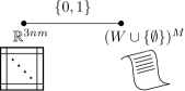
Figure 5: Raw data types for our sheaf.

These are simply the raw data spaces for each data type. Now to perform step 1, mathematization, we define the analytics on each sensor feed for the variable $L$. For sensor $C$ we have two analytics, one for $P$ (Place) and one for $L$ (vioLence). Let us consider the analytic for $L$ to be an image classification pipeline to determine probability of violence. We can consider the target space of the analytic as the following object in RV:

$$(\Omega,\mathcal{F},P) =(\mathbb{R}^{3nm},\textit{Borel sets},\textit{Image probabilities})$$

$$(S,\Sigma) =([0,1],\textit{Borel sets})$$

$$X :\mathbb{R}^{3nm}\rightarrow[0,1]$$

where the function $X$ is the result of an image classification algorithm that takes in images and returns a probability, or confidence, that the image contains violence. The “Image probabilities” would be a probability distribution over all of the images, but this should not come into play in the sheaf. We may just assume it is some probability distribution over the set of all possible images. Recall in our discussion of the RV category an assignment is simply a choice of $\omega\in\Omega$ and an $s\in S$ such that $X(\omega)=s$. Therefore, we define the analytic $f_{C,L}(\omega)=X(\omega)$.

Next we must define an analytic on $E$ (sEattle times) to inform $L$. Note that there is an additional analytic for $R$ (Role) which we will not consider. The analytic to inform $L$ from Seattle Times articles will be a bag of words model. We first map $\left(W\cup\{\emptyset\}\right)^{M}$ to $\mathbb{N}^{|W|+1}$ where each word vector is mapped to its vector of word (and empty word) occurrence counts. Then, we can further select a set $V\subseteq W$ of violent words and a disjoint set $N\subseteq W$ of non-violent (or calm) words and project the space $\mathbb{N}^{|W|+1}$ into $\mathbb{N}^{|V|+|N|}$ in the obvious fashion. Finally, we can map further into $\mathbb{N}^{2}$ by summing up all violent word occurrences and separately all non-violent word occurrences. So the full analytic is defined as $f_{E,L}(a)=[\#\text{ of violent words in article }a,\#\text{ of calm words in article }a]$.

Given our two analytics and target spaces in RV and $\mathbb{N}^{2}$ we can do step 2 of our categorification pipeline and map both target spaces into the category BOOL, the native category for variable $L$. We define

$$f_{1} :\{(\omega,s):X(\omega)=s\}\rightarrow\{0,1\}$$

$$f_{2} :\mathbb{N}^{2}\rightarrow\{0,1\}$$

where

$$f_{1}((\omega,s))=\left\{\begin{array}[]{ll}0&s<0.5\\ 1&s\geq 0.5\end{array}\right.,\qquad f_{2}((i,j)=\left\{\begin{array}[]{ll}0&i<j\\ 1&i\geq j\end{array}\right..$$

These two maps take the mathematized data space to the object $\{0,1\}\in Ob(\text{BOOL})$ so that each element of the domain maps to an element of $\{0,1\}$. Clearly these are not one-to-one functions, but that is not required. Finally, we perform step 3 using the mapping defined in the previous section to take $\{0,1\}$ to the vector space $\mathbb{R}[\{0,1\}]$.

References

• [1] Michael Barr and Charles Wells. Toposes, Triples and Theories. Number 12 in Reprints in Theory and Applications of Categories. 2005.
• [2] Robert Goldblatt. Topoi: The Categorical Analysis of Logic. Dover, 2006.
• [3] Michael Robinson. Sheaves are the canonical datastructure for sensor integration. arXiv:1603.01446v1 [math.AT].