Instability of spiral and scroll waves in the presence of a gradient in the fibroblast density: the effects of fibroblast-myocyte coupling

Abstract

Fibroblast-myocyte coupling can modulate electrical-wave dynamics in cardiac tissue. In diseased hearts, the distribution of fibroblasts is heterogeneous, so there can be gradients in the fibroblast density (henceforth we call this GFD) especially from highly injured regions, like infarcted or ischemic zones, to less-wounded regions of the tissue. Fibrotic hearts are known to be prone to arrhythmias, so it is important to understand the effects of GFD in the formation and sustenance of arrhythmic re-entrant waves, like spiral or scroll waves. Therefore, we investigate the effects of GFD on the stability of spiral and scroll waves of electrical activation in a state-of-the-art mathematical model for cardiac tissue in which we also include fibroblasts. By introducing GFD in controlled ways, we show that spiral and scroll waves can be unstable in the presence of GFDs because of regions with varying spiral or scroll-wave frequency $\omega$, induced by the GFD. We examine the effects of the resting membrane potential of the fibroblast and the number of fibroblasts attached to the myocytes on the stability of these waves. Finally, we show that the presence of GFDs can lead to the formation of spiral waves at high-frequency pacing.

• September 2016

1 Introduction

The mechanical contractions of the heart muscles are mediated by electrical waves of activation in cardiac tissue. Disturbances in the normal propagation of these electrical waves can be arryhthmogenic because of the excitation of pathological re-entrant waves, such as spiral waves, in two dimensions (2D), and scroll waves, in three dimensions (3D). Spiral waves are linked to cardiac arrhythmias, such as ventricular tachycardia (VT) and ventricular fibrillation (VF). Ventricular tachycardia is known to be associated with the existence of a single spiral (or scroll) wave in the medium [1, 2]; life-threatening VF is associated with multiple or broken spiral (or scroll) waves [3, 4, 5]. Some studies indicate that episodes of VF are preceded by VT [6, 7], suggesting the possibility of an initial onset of a spiral wave, which then degenerates to a multiple-spiral-wave turbulent state (VF) [8, 9]. Given that VF can prove to be fatal, it is important to understand this transition from VT to VF. Many factors can affect the stability of a spiral wave; hence multiple mechanisms have been proposed for this VT-VF transition [10]. Here, we discuss the effects of inhomogeneities in the fibroblast density distribution on the stability of spiral and scroll waves of electrical activation in a state-of-the-art mathematical model for cardiac tissue, in which we also include fibroblasts.

Fibroblast proliferation (fibrosis) occurs in the heart during myocardial remodelling in, e.g., ischemic hearts or hypertensive hearts [11]; such proliferation is part of the wound-healing process after injuries caused, e.g., by myocardial infarction. When fibroblasts are coupled to a cardiac myocyte, they can change the electrophysiological properties of the myocyte [12, 13, 14, 15]. This modulation of the electrophysiological properties of myocytes can, in turn, alter the dynamics of waves of electrical activation in cardiac tissue. Also, because of the heterocellular coupling between fibroblasts and myocytes, the presence of fibroblasts modulates the conduction properties of cardiac tissue. Therefore, the interposition of fibroblasts between myocytes in cardiac tissue can lead to the fragmentation of the electrical waves [16, 17] and even waveblock [17]. Many studies have investigated the effects of fibroblasts on wave dynamics in cardiac tissue [16, 17, 18, 19, 20]. Some of these studies model the fibroblasts as inexcitable obstacles [19, 20]; others take into account the fibroblast-myocyte coupling and consider either (a) a random distribution of fibroblasts, with an average density that is uniform in space [16, 17, 18], or (b) localized fibroblast inhomogeneities [18]. However, in real diseased hearts the distribution of fibroblasts may not be uniform, even on average, but, rather, there may be a gradient in fibroblast density (GFD), as has been observed in aged-rabbit hearts [6]. Moreover, in hearts that have been injured, say because of myocardial infarction, the fibroblast density may vary from a high value in the infarcted region to a lower value in the normal region of the heart [21, 22], with intermediate values in interfaces between these regions. It is important, therefore, to understand what role such GFD can play in inducing and then, perhaps, destabilizing re-entrant waves, like spiral or scroll waves.

We show that a state-of-the-art mathematical model for cardiac tissue, based on the O’Hara-Rudy model (ORd) for a human ventricular cell [23], provides us with a natural platform for (a) incorporating fibroblast-myocyte interactions and (b) imposing GFD in a controlled way so that we can study, exclusively, its effects on spiral- and scroll-wave dynamics, without other complicating factors that can be present in real cardiac tissue, such as scars, which lead to conduction inhomogeneities [24]. We carry out such a controlled study of the effects of GFD by using the ORd model, for a human ventricular cell [23], with passive fibroblasts, as in the model of MacCannell, et al. [15], which interact with myocytes (see Materials and Methods). We introduce fibroblasts in such a way that we can control GFD systematically. Before we present the details of our study, we give a qualitative overview of our principal results.

We find that GFD can destabilize spiral or scroll waves, i.e., lead to the break up of a spiral or scroll wave into multiple waves. Our in silico studies help us to uncover the principal mechanism of this GFD-induced spiral- or scroll-wave instability. The myocyte-fibroblast coupling changes the action potential duration (APD) of the attached myocytes. We show first how the spiral-wave frequency $\omega$, in a homogeneous domain with randomly distributed fibroblasts, depends inversely on the APD of the myocytes in the medium, a result that is consistent with dimensional analysis. Roughly speaking, GFD induces a gradient in the mean APD, i.e., $\overline{\rm{APD}}$, in the medium; therefore, if a spiral wave forms, with its core in a high-$\overline{\rm{APD}}$ region, its rotation frequency near the core is low. Such a low-$\omega$ region cannot support wave trains that come from a high-$\omega$ region, say because of a spiral wave there. We find that the greater the variation of $\overline{\rm{APD}}$ with GFD the more readily does spiral- or scroll-wave instability set in. We build on this qualitatively appealing argument by carrying out detailed numerical investigations of GFD-induced spiral- and scroll-wave break up, in two- and three-dimensional simulation domains, respectively, and in three models, the first with a uniform distribution of fibroblasts, and two others in which the mean density of fibroblasts changes either (a) linearly along one spatial direction or (b) as a step function. Furthermore, we investigate the effects of other fibroblast parameters, like the resting membrane potential $\rm{E_{f}}$ and the number $\rm{N_{f}}$ of fibroblasts attached to myocytes, on the stability of such spiral and scroll waves. For a given GFD, we find that the larger the values of $\rm{E_{f}}$ and $\rm{N_{f}}$, the more readily does spiral- or scroll-wave instability set in. Finally, we show how the presence of GFD can lead to the formation of re-entrant waves, like spiral waves, when we pace an edge of our simulation domain at a high frequency.

The remaining part of this paper is organized as follows. The Materials and Methods Section describes the models we use and the numerical methods we employ to study them. The Section with the title Results contains our results, from single-cell and tissue-level simulations. Finally, the Section called Discussions is devoted to a discussion of our results in the context of earlier numerical and experimental studies.

2 Materials and Methods

We use the state-of-the-art O’Hara-Rudy model (ORd) for a human ventricular cell [23] for our myocyte cell. In the ORd model, we implement the modifications suggested in Ref. [23], where the fast sodium current ($\rm{I_{Na}}$), of the original ORd model, has been replaced with that of the model due to Ten Tusscher and Panfilov [25]. The fibroblasts are modelled as passive cells, for which we use the model given by MacCannell, et al. [15], but, instead of using a constant membrane conductance $\rm{G_{f}}$, we use a $\rm{G_{f}}$ that has a nonlinear dependence on its membrane voltage $\rm{V_{f}}$, as in Refs. [16, 26]. The value of $\rm{G_{f}}$ is set to 1 nS if $\rm{V_{f}}$ is below -20 mV, and 2 nS for $\rm{V_{f}}$ above -20 mV. The gap-junctional conductance between a myocyte and a fibroblast is set to 8 nS.

In our two-dimensional (2D) simulations the fibroblasts are attached atop the myocytes; thus, our 2D simulation domain is a bilayer, as in previous studies [18, 27]; similarly, we place fibroblasts in the interstitial region between myocytes in our three-dimensional (3D) simulations as in Ref. [28]. The number of fibroblasts $\rm{N_{f}}$ attached to a myocyte in a fibroblast-myocyte composite is 2, unless otherwise mentioned in the text. For a given percentage $\rm{P_{f}}$ of fibroblasts in the medium, the fibroblasts are attached to the myocytes in a tissue with a probability $\rm{P_{f}}/100$. We carry out three types of simulations for three different models of fibroblast distribution: Model-I, Model-II, and Model-III. In Model I, the value of $\rm{P_{f}(x,y)}$ is constant throughout the domain, as in equation (1) (see figure 2 (a)). Thus, the distribution of fibroblast is uniform and isotropic. In Model II, the value of $\rm{P_{f}(x,y)}$ varies linearly along the vertical direction (y axis) of the domain (see figure 2 (b)) given by equation (2). In the last Model III, the value of $\rm{P_{f}(x,y)}$ changes discontinuously (see figure 2 (c)) given by equation (3).

$$\rm{Model~{}I:}~{}~{}~{}~{}\rm{P_{f}(x,y)}=\rm{p_{f}}~{}\forall~{}\rm{(x,y)},$$ (1)

where $\rm{p_{f}}$ is a constant between 0 and 100.

$$\rm{Model~{}II:}~{}~{}~{}~{}\rm{P_{f}(x,y)}=\rm{p_{f1}}+\frac{y(\rm{p_{f2}}-\rm{p_{f1}})}{L},0\leq\rm{y}\leq\rm{L},$$ (2)

where L is the size of the square domain, and $\rm{p_{f1}}$ and $\rm{p_{f2}}$ are constants between 0 and 100.

$$\rm{Model~{}III:}~{}~{}~{}~{}\rm{P_{f}(x,y)}=\rm{p_{f1}}\times\Theta(y_{0}-y)+\rm{p_{f2}}\times\Theta(y-y_{0}),$$ (3)

where $\Theta(\rm{y})$ is the Heaviside step function, and $\rm{y_{0}}$ is a particular value of the distance along the vertical direction; we use $\rm{y_{0}}$ = $\frac{3}{4}$L in our study.

The membrane potential of a myocyte $\rm{V_{m}}$ is governed by the ordinary differential equation (ODE)

$$\frac{{\rm{dV_{m}}}}{\rm{dt}}=-\frac{I_{\rm{ion}}+\rm{N_{f}}\times I_{\rm{gap}}}{C_{m}},$$ (4)

where $C_{m}$ is the myocyte capacitance, which has a value of 185 pF; ${I_{\rm{ion}}}$ is the sum of all the ionic currents of the myocyte, ${I_{\rm{gap}}}$ is the gap-juctional current between the fibroblast and the myocyte, and $\rm{N_{f}}$ is the number of fibroblasts attached to the myocyte. We give ${I_{\rm{ion}}}$ and ${I_{\rm{gap}}}$ below:

$$I_{\rm{ion}}=\rm{I_{Na}}+\rm{I_{to}}+\rm{I_{CaL}}+\rm{I_{CaNa}}+\rm{I_{CaK}}+\rm{I_{Kr}}+\rm{I_{Ks}}+\rm{I_{K1}}+\rm{I_{NaCa}}+\rm{I_{NaK}}+\rm{I_{Nab}}+\rm{I_{Cab}}+\rm{I_{Kb}}+\rm{I_{pCa}};$$ (5)

$$I_{\rm{gap}}=\rm{G_{gap}}(\rm{V_{m}}-\rm{V_{f}});$$ (6)

we list the ionic currents of the myocyte in Table 1.

The membrane potential of a fibroblast is governed by the equation

$$\frac{{\rm{dV_{f}}}}{\rm{dt}}=\frac{I_{\rm{gap}}-I_{\rm{f}}}{C_{f}},$$ (7)

where ${C_{f}}$=6.3 pF is the membrane capacitance of the fibroblast, and $I_{\rm{f}}$ is the fibroblast current,

$$I_{\rm{f}}=\rm{G_{f}}(\rm{V_{f}}-\rm{E_{f}});$$ (8)

here $\rm{E_{f}}$ is the resting membrane potential of the fibroblast, and its range of values in our study is from 0 to -50 mV, as observed experimentally in Refs. [26, 29, 30, 31].

Table 1: Table of currents.

$\rm{I_{Na}}$	fast inward $\rm{Na^{+}}$ current
$\rm{I_{to}}$	transient outward $\rm{K^{+}}$ current
$\rm{I_{CaL}}$	L-type $\rm{Ca^{2+}}$ current
$\rm{I_{Kr}}$	rapid delayed rectifier $\rm{K^{+}}$ current
$\rm{I_{Ks}}$	slow delayed rectifier $\rm{K^{+}}$ current
$\rm{I_{K1}}$	inward rectifier $\rm{K^{+}}$ current
$\rm{I_{NaCa}}$	$\rm{Na^{+}/Ca^{2+}}$ exchange current
$\rm{I_{NaK}}$	$\rm{Na^{+}/K^{+}}$ ATPase current
$\rm{I_{Nab}}$	$\rm{Na^{+}}$ background current
$\rm{I_{Cab}}$	$\rm{Ca^{2+}}$ background current
$\rm{I_{pCa}}$	sarcolemmal $\rm{Ca^{2+}}$ pump current
$\rm{I_{Kb}}$	$\rm{K^{+}}$ background current
$\rm{I_{CaNa}}$	$\rm{Na^{+}}$ current through the L-type $\rm{Ca^{2+}}$ channel
$\rm{I_{CaK}}$	$\rm{K^{+}}$ current through the L-type $\rm{Ca^{2+}}$ channel

A list of the ionic currents in the ORd model (symbols as in Ref. [23]).

The spatiotemporal evolution of the membrane potential ($\rm{V_{m}}$) of the myocytes in tissue is governed by a reaction-diffusion equation, which is the following partial-differential equation (PDE):

$$\frac{\partial{\rm{V_{m}}}}{\partial{t}}+\frac{I_{\rm{ion}}+\rm{N_{f}}\times I_{\rm{gap}}}{C_{m}}=\rm{D}\nabla^{2}\rm{V_{m}},$$ (9)

where $\rm{D}$ is the diffusion constant between the myocytes.

2.1 Numerical Methods

We solve the ODEs (4) and (7) for $\rm{V_{m}}$ and $\rm{V_{f}}$, respectively, and also the ODEs for the gating variables of the ionic currents of the myocyte by using a forward-Euler method. For solving the PDE (9), we use the forward-Euler method for time marching with a five-point stencil for the Laplacian in 2D and a 7-point stencil in 3D. We set D= 0.0012 $\rm{cm^{2}/ms}$. The temporal and spatial resolutions are set to be $\delta{x}$= 0.02 cm and $\delta{t}$=0.02 ms, respectively. The conduction velocity of a plane wave in the tissue, with the above set of parameters, is 65 cm/s. In our two-dimensional (2D) tissue simulations, we use a domain size of $\rm{960\times 960}$ grid points, which translates into a physical size of $\rm{19.2\times 19.2cm^{2}}$. We initiate the spiral wave by using the conventional S1-S2 cross-field protocol, where we first apply an S1 plane wave and allow its wave back to cross some part of the domain (see figure 1, time= 300 ms) and then we apply the S2 stimulus perpendicular to the S1 wave (figure 1, time= 320 ms), as shown in figure 1. The strength and duration of both the S1 and S2 stimuli are -150 $\mu\rm{A}/\mu\rm{F}$ and $3$ ms, respectively. All our tissue simulations are carried out for a duration of 10 seconds.

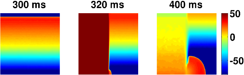
Figure 1: S1-S2 cross-field protocol. Pseudocolor plot illustrating the S1-S2 cross-field protocol that we use to initiate a spiral wave in the domain. The colorbar indicates the membrane voltage $\rm{V_{m}}$ in millivolts.

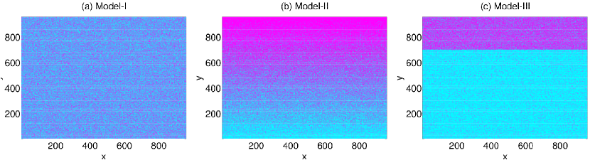
Figure 2: Models of fibroblast distribution. Pseudocolor plots showing our three models of fibroblast distribution. (a) Model-I: the density distribution of fibroblasts is uniform throughout the domain, on average. The cyan color indicates myocyte density with no fibroblasts, and the magenta color indicates fibroblast-myocyte composites. The value of $\rm{p_{f}}$ is 40%. (b) Model-II: there is a gradient of fibroblast density (GFD) along the vertical y axis, with $\rm{p_{f1}}$= 10% and $\rm{p_{f2}}$= 100% (see equation 2). (c) Model-III: $\rm{p_{f}}$ changes abruptly from 10%, in the bottom $\frac{3}{4}$ of the domain, to 70% in the upper $\frac{1}{4}$ of the domain (see equation 3).

3 Results

We first study the effects of the gap-junctional coupling $\rm{G_{gap}}$ of fibroblasts on the electrophysiological properties of myocytes. We then investigate the effects of $\rm{G_{gap}}$ on the spiral-wave frequency in a 2D simulation. Next we show how GFD leads to spiral-wave instability. Thereafter, we show the effects of GFD on scroll-wave stability in a 3D simulation domain. Finally, we discuss the role of GFD on the initiation, via pacing, of re-entrant spiral waves.

3.1 Effects of fibroblast gap-junctional coupling, on a myocyte, and the spiral-wave frequency

The gap-junctional coupling of fibroblasts with a myocyte changes the electrophysiological properties of the myocyte [12, 13, 14, 15]. For instance, it can modulate the action potential duration (APD) of a myocyte. The APD of the myocyte may increase or decrease depending on the electrophysiological properties of the fibroblasts, like their resting-membrane potential $\rm{E_{f}}$. Figure 3 shows the action potentials of a myocyte attached to $\rm{N_{f}}$= 2 fibroblasts with different values of $\rm{E_{f}}$. The APDs of the myocyte attached to fibroblasts, with $\rm{E_{f}}$= -15 mV (blue curve) and $\rm{E_{f}}$= -25 mV (black curve) are larger than that of an isolated myocyte (red curve), whereas the APD of the myocyte attached to fibroblasts with $\rm{E_{f}}$= -50 mV (magenta curve) is lower than that of an isolated myocyte.

This fibroblast-induced modulation of the APDs of the myocytes affects the properties of electrical waves, like the spiral-wave frequency, at the tissue level. This spiral frequency $\omega$ depends on the APDs of the constituent myocytes as follows. Consider a stable spiral that does not meander; dimensional analysis yields

$$\omega\simeq\frac{\theta}{\lambda},$$ (10)

where $\theta$ is the conduction velocity and $\lambda$ is the wavelength. Furthermore, $\lambda$ $\simeq$ $\theta\times\rm{APD}$, and, therefore,

$$\omega\simeq\frac{1}{\rm{APD}}.$$ (11)

In a domain with a uniform and isotropic fibroblast distribution with $\rm{P_{f}(x,y)}$=$\rm{p_{f}}$ (Model-I, equation 1 and figure 2 (a)), the average APD ($\overline{\rm{APD}}$) of the myocytes depends on $\rm{p_{f}}$, and, therefore, the frequency $\omega$ of a spiral wave depends on $\rm{p_{f}}$. In figure 5 we plot $\omega$ versus $\rm{p_{f}}$ for $\rm{E_{f}}$= -50mv (red curve), and $\rm{E_{f}}$= -25 mV (blue curve), and $\rm{E_{f}}$= -15 mV (black curve). We see from the plot for $\rm{E_{f}}$= -15 mV that $\omega$ decreases as $\rm{p_{f}}$ increases; this decrease is slower for $\rm{E_{f}}$= -25 mV; and, by the time $\rm{E_{f}}$= -50 mV, $\omega$ increases with $\rm{p_{f}}$. The decrease of $\omega$ with $\rm{p_{f}}$ for $\rm{E_{f}}$= -25 mV and -15 mV is because fibroblasts, with these values of $\rm{E_{f}}$, increase the APD of an attached myocyte (see figure 3); and, therefore, in a tissue with a uniform and isotropic fibroblast distribution, the increase of $\rm{p_{f}}$ increases $\overline{\rm{APD}}$ of the constituent myocytes, and, thereby, decreases $\omega$ (see equation (11)). However, for $\rm{E_{f}}$= -50 mV, the APD of the myocyte decreases (see figure 3), so $\omega$ increases with $\rm{p_{f}}$. For the plots in figure 5 we obtain the spiral frequency $\omega$ from the averaged power spectra of time-series of $\rm{V_{m}}$, which we record from four representative points of the domain (white squares in figure 4 (a)). We show one representative example for $\rm{p_{f}}$= 40% in figure 4. Figure 4(a) shows the spiral wave in the domain; and figure 4(b) shows the power spectrum of $\rm{V_{m}}$ averaged over those from the points (white squares in figure 4(a)) of the domain. The spiral-wave frequency $\omega$ is the value of the dominant peak in the spectrum, which is 4.4 Hz in this case.

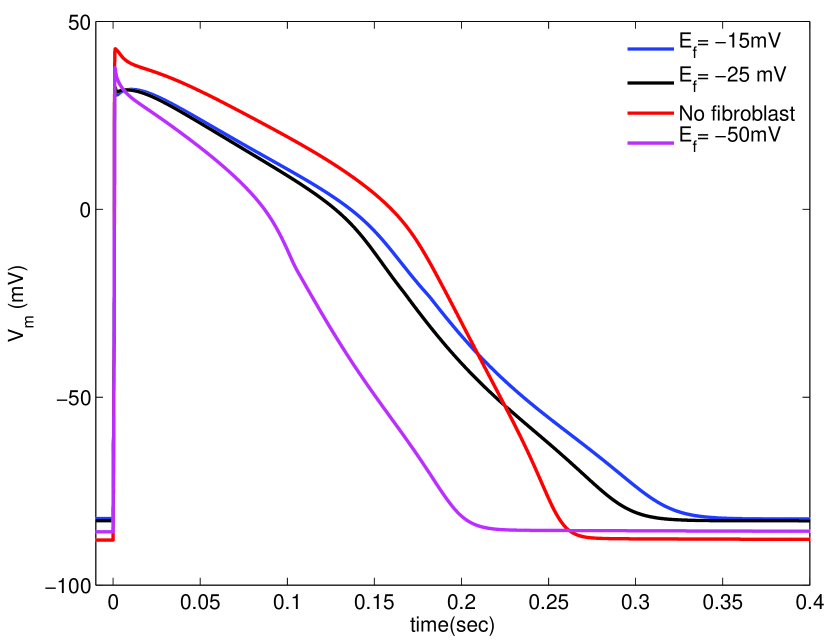
Figure 3: Action potentials of an isolated myocyte and a myocyte attached to fibroblasts. Plots showing the action potentials of an isolated myocyte (red curve), and a myocyte attached to $\rm{N_{f}}$= 2 fibroblasts of $\rm{E_{f}}$= -15 mV (blue curve), and $\rm{E_{f}}$= -25 mV (black curve), and $\rm{E_{f}}$= -50 mV (magenta curve). The APDs of the myocyte attached to fibroblasts of $\rm{E_{f}}$ = -15 mV and $\rm{E_{f}}$= -25 mV are larger than that of the isolated myocyte, whereas the APD of the myocyte attached to fibroblasts of $\rm{E_{f}}$ =-50 mV is lower than that of the isolated myocyte.

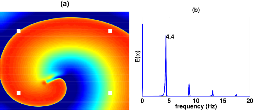
Figure 4: A spiral wave in a domain with a uniform and isotropic distribution of fibroblasts. a) The spiral wave supported in the domain with $\rm{p_{f}}$= 40%. b) The averaged power spectrum of the time-series recording of $\rm{V_{m}}$ from four representative points, indicated by white squares in (a), located near the four corners of the simulation domain. The spiral frequency $\omega$ is determined by considering the dominant peak, which is 4.4 Hz in this case; the other major peaks are harmonics at 8.8, 13.2, and 17.6 Hz.

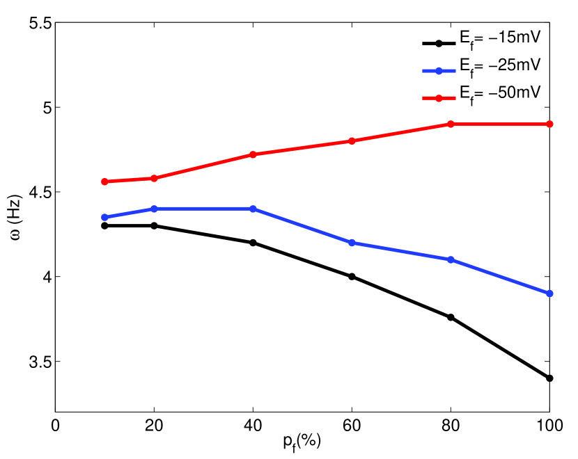
Figure 5: Variation of the spiral-wave frequency $\omega$ with the percentage of fibroblasts $\rm{p_{f}}$, in a domain with a uniform and isotropic fibroblast distribution (Model-I), for three different values of $\rm{E_{f}}$. Plots showing the variation of $\omega$ with $\rm{p_{f}}$ for $\rm{E_{f}}$= -15 mV (black curve), $\rm{E_{f}}$= -25 mV (blue curve), and $\rm{E_{f}}$= -50 mV (red curve). $\omega$ decreases with $\rm{p_{f}}$ for $\rm{E_{f}}$= -15 mV and -25 mV, but increases for $\rm{E_{f}}$= -50 mV. The variation of $\omega$ with $\rm{p_{f}}$ is most significant for $\rm{E_{f}}$= -15 mV.

3.2 Instability of spiral waves

The spiral-wave frequency $\omega$, in a domain with fibroblasts, depends on the fibroblast density $\rm{p_{f}}$. Therefore, in a domain with an inhomogeneous distribution of fibroblasts, the spiral-wave frequency (the frequency at which the spiral tip rotates) varies with space. To illustrate this, we take the Model-II fibroblast distribution (see equation 2), where $\rm{P_{f}(x,y)}$ varies along the y axis. This variation of $\rm{P_{f}(x,y)}$ in the y direction induces a y dependence in $\overline{\rm{APD}}$ and, therefore, in $\omega$. We set $\rm{p_{f1}}$= 10%, $\rm{p_{f2}}$= 80%, and $\rm{E_{f}}$= -25 mV. Figure 6 show the cases when a spiral wave is initiated in three different regions of the domain: (a) top, (b) middle, and (c) bottom. The frequencies $\omega$ of the spiral tip in these top, middle, and bottom regions are 4.2 Hz, 4.3 Hz, and 4.4 Hz, respectively. We measure these frequencies from the time series of $\rm{V_{m}}$, which we record from the four representative points, shown in figure 4 (a). The spatial dependence of the local value of $\omega$ in the domain can lead to spiral-wave instability if the variation in $\omega$ is sufficiently large. We show this for the Model-II fibroblast distribution, with $\rm{p_{f1}}$= 10%, $\rm{p_{f2}}$= 100%, and $\rm{E_{f}}$= -25 mV. If we initiate a spiral somewhere in the middle of our simulation domain, it breaks up as shown in figure 7 in the upper region of the domain, where $\omega$ is low (see also the Supplementary Video S1). This can be understood qualitatively as follows: The upper, low-$\omega$ region cannot support the high-frequency wave-trains that are emitted by the spiral tip, which is rotating in the middle region, with a higher value of $\omega$ than in the upper part of the domain; the inability of the upper region to support high-frequency waves leads to anisotropic conduction blocks because of the anisotropic fibroblast distribution and, hence, wave breaks.

This breaking of waves in the low-$\omega$ region (i.e., large $\overline{\rm{APD}}$ region) has also been observed experimentally in monolayers of neonatal-rat ventricular myocytes by Campbell, et al. [32]. In these experiments, the gradient in $\overline{\rm{APD}}$ has been induced by varying the $\rm{I_{Kr}}$ ion-channel density.

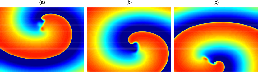
Figure 6: Variation of the spiral-wave frequency $\omega$, near the spiral tip (see text), with space in a domain with GFD. Pseudocolor plot of $\rm{V_{m}}$ showing the three cases, where the spiral wave is initiated at the top (a), middle (b), and bottom (c) parts of the domain, with a Model-II fibroblast distribution, $\rm{p_{f1}}$= 10%, $\rm{p_{f2}}$= 80%, and $\rm{E_{f}}$= -25 mV. The spiral-wave frequency $\omega$ in the top, middle, and bottom regions is 4.2 Hz, 4.3 Hz, and 4.4 Hz, respectively.

We have shown that spiral-wave instability stems from the spatial gradient in $\omega$ that is induced by the GFD. We might expect, therefore, that steep changes in $\omega$ might lead to an enhancement in such instability. To show this, we study the following two cases: case (A), with the Model-II fibroblast distribution, $\rm{p_{f1}}$= 10%, and $\rm{p_{f2}}$= 75%; and case (B), with the Model-III fibroblast distribution, given in equation 3 and illustrated in figure 2 (c), with $\rm{p_{f1}}$= 10% and $\rm{p_{f2}}$= 65%. The value of $\rm{E_{f}}$ for both these cases is -25 mV. We show in figure 8 that the spiral breaks in case (B) (figure 8 top panel), but not in case (A) (figure 8 bottom panel), although the maximum fibroblast percentage is higher in case (A), with the Model-II distribution, than in case (B), with the Model-II distribution (see also the Supplementary Video S2). Therefore, a comparison of our results for cases (A) and (B) shows that a high local slope of $\frac{\rm{d\omega}}{\rm{dy}}$, which has a singularity at y= $\frac{3}{4}$L in Model-III, enhances spiral-wave instability.

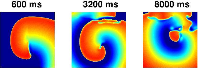
Figure 7: Spiral-wave instability in the presence of GFD. Pseudocolor plot of $\rm{V_{m}}$ showing the spatiotemporal evolution of the break-up of a spiral in the presence of GFD, with the Model-II distribution (figure 2 (b)), $\rm{p_{f1}}$= 10%, $\rm{p_{f2}}$= 100%, and $\rm{E_{f}}=$ -25 mV. The spiral arm breaks up in the upper region, where the spiral frequency $\omega$ supported by the region is lower than that in the bottom region.

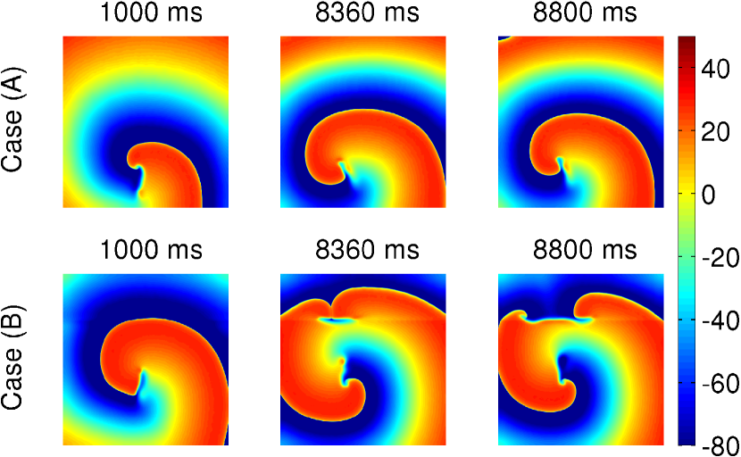
Figure 8: Dependence of spiral-wave stability on the value of the gradient of $\omega$ induced by the GFD. Pseudocolor plot of $\rm{V_{m}}$ showing the spatiotemporal evolution of a spiral for two cases (A) and (B) of the fibroblast distribution. Top-panel figures show a stable spiral for case (A), with the Model-II fibroblast distribution, $\rm{p_{f1}}$= 10%, and $\rm{p_{f2}}$= 75%. The bottom panels shows spiral break-up for case (B), with the Model-III fibroblast distribution, $\rm{p_{f1}}$= 10%, and $\rm{p_{f2}}$= 65% in equation 3.

Dependence of spiral-wave instability on fibroblast parameters

The APD of a myocyte, in a fibroblast-myocyte composite, depends on $\rm{E_{f}}$, and, therefore, the stability of a spiral wave in a domain with GFD also depends on $\rm{E_{f}}$. To illustrate this, we first recall the variation of $\omega$ with $\rm{p_{f}}$ for three values of $\rm{E_{f}}$ in figure 5, namely, $\rm{E_{f}}$= -15 mV (black curve), $\rm{E_{f}}$= -25 mV (blue curve), and $\rm{E_{f}}$= -50 mV (red curve). Note that the change in $\omega$ with $\rm{p_{f}}$ is more significant for $\rm{E_{f}}$= -15 mV than for $\rm{E_{f}}$= -25 mV. Therefore, in a domain with a given GFD, the spiral breaks up with a lower GFD for $\rm{E_{f}}$= -15 mV than for $\rm{E_{f}}$= -25 mV. Figure 9 (top panel) shows the break-up of a spiral wave for GFD with the Model-II distribution, $\rm{p_{f1}}$= 10%, $\rm{p_{f2}}$=80%, and $\rm{E_{f}}$= -15 mV. The same GFD does not lead to spiral-wave break-up for $\rm{E_{f}}$= -25 mV (figure 9, bottom panel) (see also the Supplementary Video S3). This indicates that the readiness with which spiral-wave instability sets in depends on the degree of variation of $\omega$ induced by the GFD. For $\rm{E_{f}}$= -50 mV, $\omega$ decreases with $\rm{p_{f}}$ (figure 5). Therefore, in the presence of GFD, with the Model-II distribution, $\rm{p_{f1}}$= 10% and $\rm{p_{f2}}$= 100%, the spiral breaks up in the bottom region of the domain, as shown in figure 10 (see also the Supplementary Video S4). This demonstrates again that the waves break in the low-$\omega$ region of the domain.

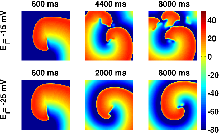
Figure 9: Dependence of spiral-wave stability on $\rm{E_{f}}$. Pseudocolor plot of $\rm{V_{m}}$ showing the break-up of a spiral in the presence of GFD, with the Model-II distribution, $\rm{p_{f1}}$= 10%, and $\rm{p_{f2}}$=80% for $\rm{E_{f}}$= -15mV (top panel); the same GFD does not lead to break-up for $\rm{E_{f}}$= -25 mV (bottom panel).

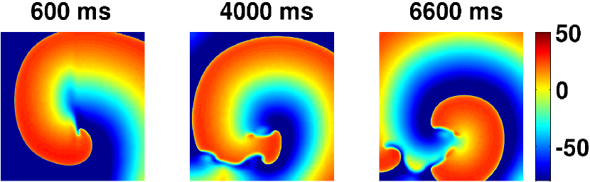
Figure 10: Spiral-wave break-up in the presence of GFD, with $\rm{E_{f}}$= -50 mV. Pseudocolor plot of $\rm{V_{m}}$ showing the break-up of a spiral in the presence of GFD with the Model-II distribution, $\rm{p_{f1}}$=10%, $\rm{p_{f2}}$=100%, and $\rm{E_{f}}$= -50 mV. The spiral breaks up in the bottom part of the domain because it is the low-$\omega$ region.

The variation of $\omega$ with $\rm{p_{f}}$ also depends on the number $\rm{N_{f}}$ of fibroblasts that are attached to the myocytes. Figure 11 shows the variation of $\omega$ with $\rm{p_{f}}$ for different values of $\rm{N_{f}}$, for a constant value of $\rm{E_{f}}$= -15 mV. The black, blue, and red curves are for $\rm{N_{f}}$= 1, 2, and 3, respectively. These plots show that the larger the value of $\rm{N_{f}}$ the larger is the change of $\omega$ with $\rm{p_{f}}$. Hence, in a domain with a given GFD and $\rm{E_{f}}$, the spiral-wave instability increases with $\rm{N_{f}}$, because the variation of $\omega$ with $\rm{p_{f}}$ increases with $\rm{N_{f}}$. To illustrate this, figure 12 (top panel) shows the breaking of a spiral wave for a GFD with the Model-II distribution, $\rm{p_{f1}}$= 10%, $\rm{p_{f2}}$= 60%, $\rm{E_{f}}$= -15 mV, and $\rm{N_{f}}$= 3. The same GFD and $\rm{E_{f}}$ does not lead to spiral break-up for $\rm{N_{f}}$= 2 (figure 12, bottom panel). (See also the Supplementary Video S5.)

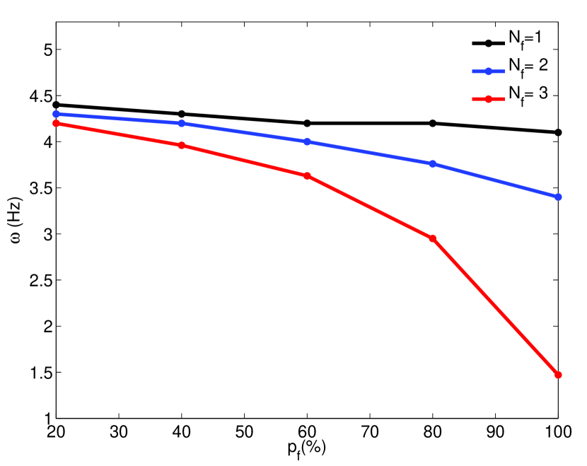
Figure 11: Variation of the spiral-wave frequency $\omega$ with $\rm{p_{f}}$ for different values of $\rm{N_{f}}$. A plot showing the variation of $\omega$ with $\rm{p_{f}}$ for three different values of $\rm{N_{f}}$: $\rm{N_{f}}$= 1 (black curve), 2 (blue curve), and 3 (red curve). The value of $\rm{E_{f}}$ is held constant at -15 mV for all the curves. The variation of $\omega$ with $\rm{p_{f}}$ is most significant for $\rm{N_{f}}$= 3.

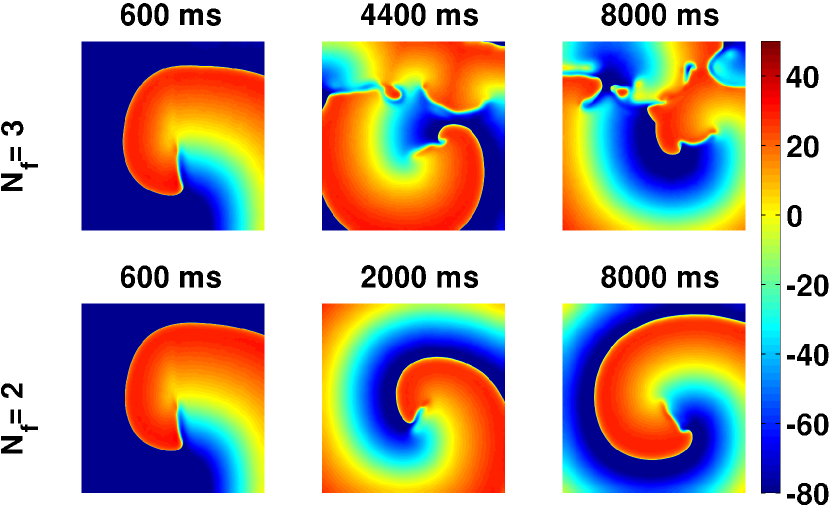
Figure 12: Dependence of spiral-wave stability on $\rm{N_{f}}$. Pseudocolor plots of $\rm{V_{m}}$ showing the break-up of a spiral in the presence of GFD with the Model-II distribution, $\rm{p_{f1}}$=10%, and $\rm{p_{f2}}$=60%, for $\rm{E_{f}}$= -15 mV and $\rm{N_{f}}$= 3 (top panel). The same GFD and $\rm{E_{f}}$ does not lead to break-up for $\rm{N_{f}}$= 2 (bottom panel).

3.3 Three-dimensional simulation domains

To check if our results also hold in 3D simulation domains, we perform a few representative 3D simulations, where the thickness (x dimension) is 2 mm and the linear dimensions in the y and z directions are both 19.2 cm. We initiate a scroll wave by using the same S1-S2 cross-field protocol that we use in our 2D simulations for spiral-wave initiation. We find that the results we obtain in 3D, for the dependence of scroll-wave stability on $\rm{E_{f}}$ and $\rm{N_{f}}$, are qualitatively similar to those we have obtained above for spiral-wave stability in 2D. For example, we show the dependence of scroll-wave stability on $\rm{N_{f}}$. We take a 3D domaim with GFD given by the Model-II fibroblast distribution: $\rm{P_{f}(x,y,z)}$ varies from $\rm{p_{f1}}$= 10% to $\rm{p_{f2}}$= 60% along the z axis, but is constant in the x-y plane for a fixed value of z; we use $\rm{E_{f}}=$-15 mV here. Now we study the stability of a scroll wave for $\rm{N_{f}}$= 2 and $\rm{N_{f}}$= 3. Figure 13(a) shows a scroll wave breaking up for $\rm{N_{f}}$= 3; however, the scroll does not break up for $\rm{N_{f}}$= 2, as shown in figure 13(b) (see also the Supplementary Video S6). Therefore, with GFD, the higher the value of $\rm{N_{f}}$ the greater is the instability of scroll waves (as in our 2D simulations).

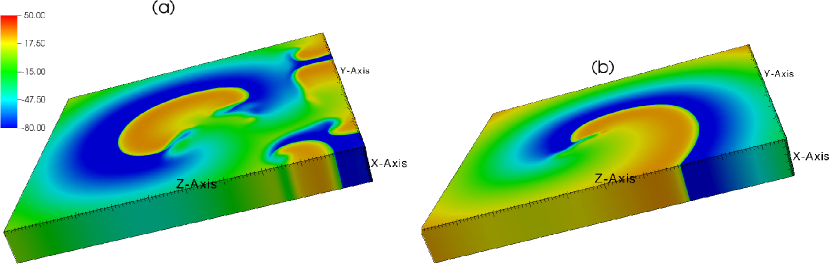
Figure 13: Dependence of scroll-wave stability on $\rm{N_{f}}$. Pseudocolor plots of $\rm{V_{m}}$ showing the stability of scroll waves in a 3D domain with GFD (Model-II distribution, with $\rm{P_{f}(x,y,z)}$ varying from $\rm{p_{f1}}$= 10% to $\rm{p_{f2}}$= 60% along the z-axis and constant in the x-y plane for a fixed value of z). The value of $\rm{E_{f}}$ is set to -15 mV. (a) The scroll wave breaks up for $\rm{N_{f}}$=3; (b) the scroll wave remains stable for $\rm{N_{f}}$=2.

3.4 Pacing-induced re-entry

So far we have discussed the stability of spiral and scroll waves in the presence of GFD, where we initiate the spiral or scroll waves by using the S1-S2 cross-field protocol. We now show GFD itself can lead to re-entry (i.e., the formation of spiral or scroll waves) if we pace the system. To illustrate this, we pace our 2D simulation at a high frequency, with a pacing cycle length PCL= 250 ms, in the presence of GFD (the Model-II fibroblast distribution, $\rm{p_{f1}}$= 10%, $\rm{p_{f2}}$= 100%, and $\rm{E_{f}}$= -15 mV). The pacing stimulus is applied at the bottom edge of the domain. We apply 20 pulses with this PCL, and we observe that a spiral wave is induced by such high-frequency pacing, as shown in figure 14 (see also the Supplementary Video S7). Thus, GFD not only provides a substrate for spiral- or scroll- wave instabilities in cardiac tissue, but it can also be a source of such re-entrant waves if the tissue is paced at sufficiently high frequency. Such pacing-induced spiral waves occur with high-frequency pacing (low PCL) but not with low-frequency (large PCL) pacing. In the stability diagram of figure 15, we show the region in which we observe such pacing-induced re-entry in the $\rm{E_{f}}$-PCL plane in the presence of the GFD. The black-colored region indicates the region in which we obtain spiral waves, and the red-colored region is the region in which we do not see spiral waves. Thus, for a given $\rm{E_{f}}$, re-entry occurs below a certain PCL; and, as $\rm{E_{f}}$ decreases, the threshold of PCL, below which re-entry occurs, decreases. Re-entry occurs with high-frequency and not with low-frequency pacing for the following reasons. The wavebacks of the travelling waves repolarize (come back to the resting state) slowly in the low-$\omega$ regions, which are in the top part of our simulation domain in figure 14, because $\overline{\rm{APD}}$ is large in these regions. When we use low-frequency pacing, the wave-fronts do not meet the wavebacks of the preceding waves. By contrast, when we use high-frequency pacing, the wavefronts of the succeeding waves interact with the wavebacks of the preceding waves, and, because of the anisotropic repolarization that arises from the GFD, the succeeding wavefronts become corrugated, which leads to re-entry and the formation of spiral waves.

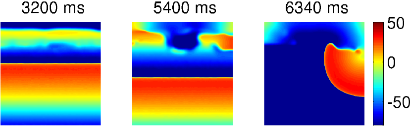
Figure 14: Pacing-induced spiral wave. Pseudocolor plot of $\rm{V_{m}}$ showing the pacing-induced occurrence of a spiral wave, in a 2D simulation domain with GFD (the Model-II distribution, $\rm{p_{f1}}$= 10%, and $\rm{p_{f2}}$= 100% GFD) paced with PCL= 250 ms. The pacing stimuli are applied at the bottom of the domain.

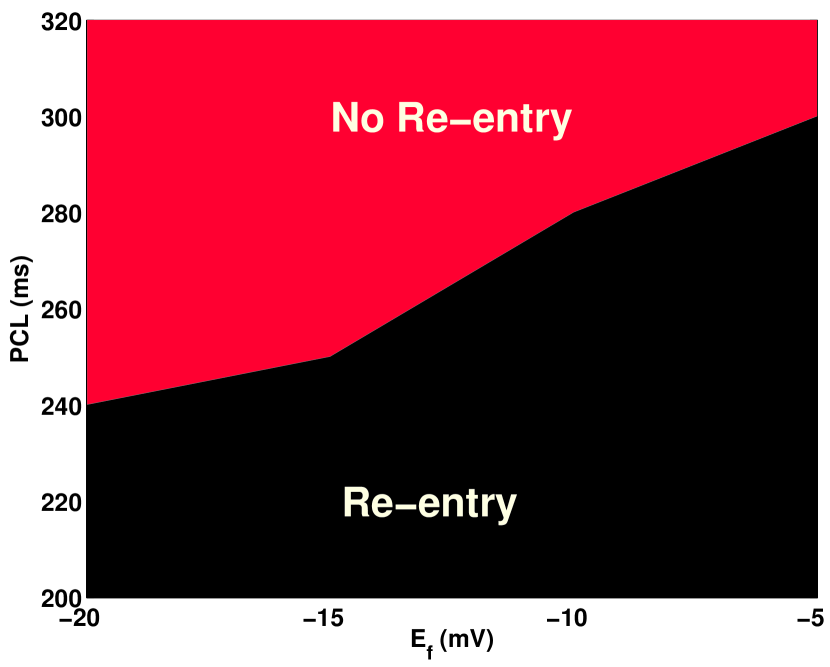
Figure 15: Stability diagram in the $\rm{E_{f}}$-PCL plane. Figure showing the re-entry (black) and no re-entry (red) regions in the $\rm{E_{f}}$-PCL plane (see text). This figure shows that re-entry occurs in the low-PCL region; and, as $\rm{E_{f}}$ decreases, the threshold PCL, below which re-entry occurs, also decreases.

4 Discussion

We have shown by detailed numerical simulations how gradients in the fibroblast density (GFD) affect spiral- or scroll-wave dynamics in the state-of-the-art ORd mathematical model for cardiac tissue. Our work shows that such gradients induce spatial variations in the local spiral- or scroll-wave frequency $\omega$. These variations play a crucial role in the stability of these spiral or scroll waves in the presence of GFD. In particular, we find that spiral or scroll waves break in regions where the local $\omega$ is low. Furthermore, for a particular GFD, the stability of these waves depend on $\rm{E_{f}}$ and $\rm{N_{f}}$, insofar as they affect the variation of $\omega$ with $\rm{p_{f}}$ (see figures 5 and 11). Last, but not least, high-frequency pacing at one end of our domain can lead to the formation of spiral waves if GFD is present.

Some earlier studies have investigated the effects of fibroblasts on spiral- and scroll-wave dynamics. Numerical simulations of mathematical models of cardiac tissue, with a distribution of fibroblasts, have shown single or multiple spiral or scroll waves [17], depending on the fibroblast density. A detailed study of the effects of homogeneous or localized distributions of fibroblasts on spiral-wave dynamics has been carried out by Nayak, et al. [18]. Fibroblasts, randomly distributed, have been shown to convert complex wave patterns, like mutiple-spiral states, to simpler patterns, like a single rotating spiral state [28]. In a mathematical model of heart-failure tissue, Gomez, et al., have found that the presence of fibroblasts enhances re-entrant phenomena [33]. Also, the fibroblast-myocyte coupling has been found to be arrythmogenic, because of its ability to induce pathological excitations, like alternans [12] and early afterdepolarizations [6]; the latter can, in turn, lead to re-entries.

Although these studies, and many others [19, 20, 21], have investigated the causes of re-entrant waves and their sustenance in cardiac tissue with fibroblasts, none of them has studied, systematically, spiral- and scroll-wave instability because of the fibroblast-myocyte coupling in a domain with GFD. Our study, in which we control GFD, has allowed us to study clearly the arrhythmogenic potential of such GFD. It is important to carry out such an investigation because the gradients in density distribution of fibroblasts are known to occur in real hearts [6]. We hope our results will lead to detailed studies of GFD-induced spiral- and scroll-wave instability at least in in vitro experiments on cell-cultures. At the simplest level, we suggest fibroblast analogs of the experiments of Campbell, et al. [32], in which the gradient in $\overline{\rm{APD}}$ has been induced by varying the $\rm{I_{Kr}}$ ion-channel density.

We end our discussion with some limitations of our study. Our tissue simulations do not take into account anisotropy because of the orientation of muscle fibers. Such tissue anisotropy may exacerbate the instability of spiral waves in the presence of a GFD. We have used a monodomain representation of cardiac tissue; our study needs to be extended to other tissue models, such as those that use bidomain representations [34]. We use a passive model of the fibroblasts; however, there is some evidence [15, 35, 36], that fibroblasts can behave as active cells. Nonetheless, our qualitative results, about the arrhythmogenic effects of GFD, and its root cause, should not depend on such details.

Supplementary Data

Video S1. Video showing the break-up of a spiral in the presence of GFD, with the Model-II distribution, $\rm{p_{f1}}$= 10%, and $\rm{p_{f2}}$=100% for $\rm{E_{f}}$= -25mV. We use 10 frames per second with each frame separated from the succeeding frame by 20ms in real time. (MPEG)

Video S2. Video showing the spatiotemporal evolution of a spiral for two cases (A) and (B) of the fibroblast distribution. The video on the left-panel shows a stable spiral for case (A), with the Model-II fibroblast distribution, $\rm{p_{f1}}$= 10%, and $\rm{p_{f2}}$= 75%. The right-panel video shows spiral break-up for case (B), with the Model-III fibroblast distribution, $\rm{p_{f1}}$= 10%, and $\rm{p_{f2}}$= 65%. We use 10 frames per second with each frame separated from the succeeding frame by 20ms in real time. (MPEG)

Video S3. Video showing the break-up of a spiral in the presence of GFD, with the Model-II distribution, $\rm{p_{f1}}$= 10%, and $\rm{p_{f2}}$=80% for $\rm{E_{f}}$= -15mV (right panel); the same GFD does not lead to break-up for $\rm{E_{f}}$= -25 mV (left panel). We use 10 frames per second with each frame separated from the succeeding frame by 20ms in real time. (MPEG)

Video S4. Video showing the break-up of a spiral in the presence of GFD with the Model-II distribution, $\rm{p_{f1}}$=10%, $\rm{p_{f2}}$=100%, and $\rm{E_{f}}$= -50 mV. The spiral breaks up in the bottom part of the domain because it is the low-$\omega$ region. We use 10 frames per second with each frame separated from the succeeding frame by 20ms in real time. (MPEG)

Video S5. Video showing the break-up of a spiral in the presence of GFD with the Model-II distribution, $\rm{p_{f1}}$=10%, and $\rm{p_{f2}}$=60%, for $\rm{E_{f}}$= -15 mV and $\rm{N_{f}}$= 3 (left panel). The same GFD and $\rm{E_{f}}$ does not lead to break-up for $\rm{N_{f}}$= 2 (right panel). We use 10 frames per second with each frame separated from the succeeding frame by 20ms in real time. (MPEG)

Video S6. Video (bottom panel) showing the break-up of a scroll wave in a 3D domain with GFD (Model-II distribution, with $\rm{P_{f}(x,y,z)}$ varying from $\rm{p_{f1}}$= 10% to $\rm{p_{f2}}$= 60% along the z-axis and constant in the x-y plane for a fixed value of z), where the value of $\rm{E_{f}}$ is set to -15 mV and $\rm{N_{f}}$=3. The same GFD and $\rm{E_{f}}$ does not lead to break up for $\rm{N_{f}}$=2 (top panel). We use 10 frames per second with each frame separated from the succeeding frame by 20ms in real time. (MPEG)

Video S7. Video showing the pacing-induced occurrence of a spiral wave, in a 2D simulation domain with GFD (the Model-II distribution, $\rm{p_{f1}}$= 10% and $\rm{p_{f2}}$= 100% GFD, and $\rm{E_{f}}$= -25 mV) paced with PCL= 250 ms. We use 10 frames per second with each frame separated from the succeeding frame by 20ms in real time. (MPEG)

References

References

- [1] Efimov I R, Sidorov V, Cheng Y and Wollenzier B 1999 Journal of cardiovascular electrophysiology 10 1452–1462
- [2] De Bakker J, Van Capelle F, Janse M, Wilde A, Coronel R, Becker A, Dingemans K, Van Hemel N and Hauer R 1988 Circulation 77 589–606
- [3] Bayly P, KenKnight B, Rogers J, Johnson E, Ideker R and Smith W 1998 Chaos: An Interdisciplinary Journal of Nonlinear Science 8 103–115
- [4] Witkowski F X, Leon L J, Penkoske P A, Giles W R, Spano M L, Ditto W L and Winfree A T 1998 Nature 392 78–82
- [5] Walcott G P, Kay G N, Plumb V J, Smith W M, Rogers J M, Epstein A E and Ideker R E 2002 Journal of the American College of Cardiology 39 109–115
- [6] Morita N, Sovari A A, Xie Y, Fishbein M C, Mandel W J, Garfinkel A, Lin S F, Chen P S, Xie L H, Chen F et al. 2009 American Journal of Physiology-Heart and Circulatory Physiology 297 H1594–H1605
- [7] Mäkikallio T H, Koistinen J, Jordaens L, Tulppo M P, Wood N, Golosarsky B, Peng C K, Goldberger A L and Huikuri H V 1999 The American journal of cardiology 83 880–884
- [8] Courtemanche M 1996 Chaos: An Interdisciplinary Journal of Nonlinear Science 6 579–600
- [9] Karma A 1993 Physical review letters 71 1103
- [10] Fenton F H, Cherry E M, Hastings H M and Evans S J 2002 Chaos: An Interdisciplinary Journal of Nonlinear Science 12 852–892
- [11] Manabe I, Shindo T and Nagai R 2002 Circulation research 91 1103–1113
- [12] Xie Y, Garfinkel A, Weiss J N and Qu Z 2009 American Journal of Physiology-Heart and Circulatory Physiology 297 H775–H784
- [13] Nguyen T P, Xie Y, Garfinkel A, Qu Z and Weiss J N 2012 Cardiovascular research 93 242–251
- [14] Sachse F B, Moreno A P, Seemann G and Abildskov J 2009 Annals of biomedical engineering 37 874–889
- [15] MacCannell K A, Bazzazi H, Chilton L, Shibukawa Y, Clark R B and Giles W R 2007 Biophysical journal 92 4121–4132
- [16] Zlochiver S, Munoz V, Vikstrom K L, Taffet S M, Berenfeld O and Jalife J 2008 Biophysical journal 95 4469–4480
- [17] Majumder R, Nayak A R and Pandit R 2012
- [18] Nayak A R, Shajahan T, Panfilov A and Pandit R 2013 PLoS One 8 e72950
- [19] Ten Tusscher K H and Panfilov A V 2007 Europace 9 vi38–vi45
- [20] Kazbanov I V, Ten Tusscher K H and Panfilov A V 2016 Scientific reports 6
- [21] Nguyen T P, Qu Z and Weiss J N 2014 Journal of molecular and cellular cardiology 70 83–91
- [22] Ashikaga H, Arevalo H, Vadakkumpadan F, Blake R C, Bayer J D, Nazarian S, Zviman M M, Tandri H, Berger R D, Calkins H et al. 2013 Heart Rhythm 10 1109–1116
- [23] O’Hara T, Virág L, Varró A and Rudy Y 2011 PLoS Comput Biol 7 e1002061
- [24] Shajahan T, Nayak A R and Pandit R 2009 PLoS One 4 e4738
- [25] ten Tusscher K H and Panfilov A V 2006 American Journal of Physiology-Heart and Circulatory Physiology 291 H1088–H1100
- [26] Rook M, Van Ginneken A, de Jonge B, El Aoumari A, Gros D and Jongsma H 1992 American Journal of Physiology-Cell Physiology 263 C959–C977
- [27] Zimik S, Nayak A R and Pandit R 2015 PloS one 10 e0144979
- [28] Nayak A R and Pandit R 2015 Physical Review E 92 032720
- [29] Camelliti P, Borg T K and Kohl P 2005 Cardiovascular research 65 40–51
- [30] Kamkin A, Kiseleva I, Wagner K, Lammerich A, Bohm J, Persson P and Günther J 1999 Experimental Physiology 84 347–356
- [31] Kohl P 2003 Circulation research 93 381–383
- [32] Campbell K, Calvo C J, Mironov S, Herron T, Berenfeld O and Jalife J 2012 The Journal of physiology 590 6363–6379
- [33] Gomez J F, Cardona K, Martinez L, Saiz J and Trenor B 2014 PloS one 9 e103273
- [34] Henriquez C S 1992 Critical reviews in biomedical engineering 21 1–77
- [35] Li G R, Sun H Y, Chen J B, Zhou Y, Tse H F and Lau C P 2009 PLoS One 4 e7307–e7307
- [36] Jacquemet V and Henriquez C S 2007 Europace 9 vi29–vi37