Uncertainty quantification for generalized Langevin dynamics

Abstract

We present efficient finite difference estimators for goal-oriented sensitivity indices with applications to the generalized Langevin equation (GLE). In particular, we apply these estimators to analyze an extended variable formulation of the GLE where other well known sensitivity analysis techniques such as the likelihood ratio method are not applicable to key parameters of interest. These easily implemented estimators are formed by coupling the nominal and perturbed dynamics appearing in the finite difference through a common driving noise, or common random path. After developing a general framework for variance reduction via coupling, we demonstrate the optimality of the common random path coupling in the sense that it produces a minimal variance surrogate for the difference estimator relative to sampling dynamics driven by independent paths. In order to build intuition for the common random path coupling, we evaluate the efficiency of the proposed estimators for a comprehensive set of examples of interest in particle dynamics. These reduced variance difference estimators are also a useful tool for performing global sensitivity analysis and for investigating non-local perturbations of parameters, such as increasing the number of Prony modes active in an extended variable GLE.

I Introduction

Sensitivity analysis (SA), understanding how changes in input parameters affect the output of a system, is a key component of uncertainty quantification (UQ), optimal experimental design, and analysis of model robustness, identifiability, and reliability. Saltelli, Tarantola, and Campolongo (2000); Saltelli et al. (2000) The local sensitivity of a system can be analyzed by computing sensitivity indices that are formed by taking partial derivatives with respect to each of the input parameters. These indices quantify which parameter directions are most sensitive to perturbations.

The present articles concerns SA techniques for the GLE and other models of interest in particle dynamics. The Langevin equation (LE) models particle diffusion in the presence of a heat bath where the particle-bath interactions are reduced to an instantaneous drag force and a delta-correlated random force.Coffey and Kalmykov (2012) This approximation dramatically reduces the computational cost compared to explicitly resolving the particle-bath interactions. However, there are a number of compelling applications where the Langevin assumptions fail to produce a reliable model, such as anomalous diffusion. The GLE, a more reliable model of anomalous diffusion, incorporates “memory” into the drag force through the inclusion of a kernel depending on the history of the velocity. In many instances, this non-Markovian system can be mapped onto a Markovian system with additional degrees of freedom under physically reasonable assumptions, such as when the memory kernel can be approximated by a positive Prony series.Baczewski and Bond (2013) The resulting extended variable formulation contains many parameters that must be tuned and is therefore an ideal candidate for SA and UQ. However, well known SA techniques such as likelihood ratio and pathwise methods are not applicable to analyze the sensitivity of key parameters of interest in the extended variable formulation. In contrast, Monte Carlo finite difference estimators of sensitivity indices are applicable to all parameters of interest in the extended variable GLE, but introduce a bias error and typically have a large variance making them computationally expensive.

We give efficient Monte Carlo finite difference estimators via a coupling method for approximating goal-oriented sensitivity indices for a large class of SDEs. In particular, we apply these estimators to an extended variable formulation of the GLE where the memory kernel can be approximated by a positive Prony series, a choice motivated by applications in anomalous diffusion in biological fluids.Mason and Weitz (1995); Goychuk (2012) In the context of this application area, we mention that other authors have given a Bayesian methodology for comparing different models of anomalous diffusion that favors the GLE.Lysy et al. (2016) In addition to biological fluids, other recent interesting applications of the GLE include: modeling nanoscale materials and solids; Kantorovich (2008); Kantorovich and Rompotis (2008); Stella, Lorenz, and Kantorovich (2014); Ness et al. (2015, 2016) thermostats for sampling classical and path integral molecular dynamics;Ceriotti, Manolopoulos, and Parrinello (2011); Morrone et al. (2011); Ceriotti, Bussi, and Parrinello (2010); Ceriotti et al. (2010); Ceriotti, Bussi, and Parrinello (2009a, b) and, more generally, reduced order modeling.Chorin and Stinis (2007); Hijón et al. (2010); Darve, Solomon, and Kia (2009); Li et al. (2015) This list of applications is far from exhaustive but nevertheless provides strong incentive for investigating SA and UQ techniques for the GLE and its extended variable formulations.

To provide further orientation consider, for simplicity, the sensitivity of the stochastic dynamics $X_{t}(\theta)$, depending on an input parameter $\theta$,

$$\mathcal{S}(t,\theta;f)=\partial_{\theta}\operatorname{\mathbf{E}}[f(X_{t}(\theta))],$$

for a given observable $f$ where $\partial_{\theta}$ is the derivative with respect to $\theta$. In general, the finite difference approach is to approximate the derivative above by a finite difference quotient and then obtain the required moments by Monte Carlo. For example, a forward difference with bias parameter $\varepsilon$ yields the sensitivity estimator,

$$\mathcal{S}_{\varepsilon}(t,\theta;f)=\left(\operatorname{\mathbf{E}}[f(X_{t}(\theta+\varepsilon))]-\operatorname{\mathbf{E}}[f(X_{t}(\theta))]\right)/\varepsilon,$$ (1)

where $\mathcal{S}_{\varepsilon}\approx\mathcal{S}$ for $\varepsilon$ small, and then the estimator is computed by approximating the expectations with sample averages. Similar expressions can be given for central differences and more general finite difference stencils. While this approach requires little analysis of the underlying model and is easily implemented, the introduction of the bias, and in particular its effect on the variance of $\mathcal{S}_{\varepsilon}$, a key quantity in evaluating the efficiency of the method, is often cited as a reason for pursuing alternative methods.Chen and Glasserman (2007) However, as we shall show, the variance of $\mathcal{S}_{\varepsilon}$ can be reduced by choosing the right sampling strategy for the observable of the nominal and perturbed dynamics, respectively, $f(X_{t}(\theta))$ and $f(X_{t}(\theta+\varepsilon))$ in the expression above. For a comprehensive set of examples of interest in particle dynamics, we demonstrate that coupling the nominal and perturbed dynamics through a common driving noise, that is, a common random path coupling, reduces the variance of the finite difference estimator, often substantially. In particular, for the extended variable GLE with a convex potential the reduction due to the common random path coupling is on the order of the bias squared—mitigating the effect of the systematic error. The common random path coupling also leads to reduced variance estimators for problems with nonconvex potentials, although the reduction is not expected to be on the order of the bias squared (cf. Figures 4 and 5). This is a topic that deserves further rigorous analysis that will be the subject of future work.

Other well known SA techniques for continuous time stochastic dynamics, including pathwise methods, Pantazis and Katsoulakis (2013) likelihood ratio methods, Glynn (1990); Arampatzis, Katsoulakis, and Rey-Bellet (2016) and Malliavin methods,Fournié et al. (1999, 2001) produce unbiased estimators of sensitivity indices by representing $\mathcal{S}$ as the expectation of $f$ (or its derivative) under a change of measure. A very good account of the interrelations among them has been given by other authors.Chen and Glasserman (2007) However, each of these methods is not suited to our application of interest, the GLE, for reasons that we detail below.

The pathwise and likelihood ratio methods are not applicable to key parameters of interest, those appearing in the drift and diffusion terms, in the extended variable formulation of the GLE. The pathwise method views the dynamics at each fixed time as a density and takes a derivative of this density yielding the estimator, $\mathcal{S}_{P}(t,\theta;f)=\partial_{\theta}\operatorname{\mathbf{E}}[f(X_{t}(\theta))]=\operatorname{\mathbf{E}}\left[f^{\prime}(X_{t}(\theta))\partial_{\theta}X_{t}(\theta)\right],$ requiring equality to hold when the order of differentiation and expectation are interchanged and a smooth observable $f$. In its most general form, if an expression $\operatorname{\mathbf{E}}[f(X_{t}(\theta))]=\int f(x_{t})g(\theta,x_{t})\mathrm{d}x_{t}$ exists, then the likelihood ratio estimator,

$$\mathcal{S}_{LR}(t,\theta;f) =\partial_{\theta}\operatorname{\mathbf{E}}[f(X_{t}(\theta))]$$

$$=\int f(x_{t})\left[\partial_{\theta}\log g(\theta,x_{t})\right]g(\theta,x_{t})\mathrm{d}x_{t}$$

$$=\operatorname{\mathbf{E}}\left[f(X_{t}(\theta))\partial_{\theta}\log g(\theta,X_{t})\right],$$

is obtained by bringing the derivative inside the integral and multiply and dividing by $g$. However, this formulation requires knowledge of the unknown density $g$ and, in practice, pathwise information is substituted: $\mathcal{S}_{LR}(t,\theta;f)\approx\operatorname{\mathbf{E}}[f(X_{t}(\theta))G(\{X_{s}\}_{0\leq s\leq t})]$. For both estimators, the application of these methods to key parameters of interest in the extended variable formulation of the GLE leads to perturbations in path-space that are not absolutely continuous, that is, the typical Girsanov change of measure does not hold in path-space.

An approach that circumvents this lack of a Girsanov transform for certain parameters, using the Malliavin derivativeNualart (2006), first appeared in finance applications for calculating sensitivities, known as Greeks, related to the pricing of certain securities. Fournié et al. (1999, 2001); Bouchard, Ekeland, and Touzi (2004) Applied directly to continuous time dynamics, the Malliavin approach produces unbiased estimators $\mathcal{S}_{M}=\operatorname{\mathbf{E}}[f(X_{T})h(\{X_{s}\}_{0\leq s\leq T})]$ where $h$ is a non-unique weight that involves a system of auxiliary processes obtained through Malliavin calculus but that does not depend on $g$. In particular, for overdamped Langevin dynamics Malliavin weights are given for sensitivities with respect to parametric forces, that is, for parameters appearing in the drift term only.Warren and Allen (2012) While in principle the Malliavin method applies to other perturbations that cannot be handled by pathwise and likelihood ratio methods, it requires a number of auxiliary processes that may scale poorly with the system size and is not clearly computationally practical for the extended variable GLE.

We mention that, finite differences using common random numbers have been employed, based on empirical evidence, for SA with respect to parametric forces for the LE.Assaraf et al. (2015); Ciccotti and Jacucci (1975); Stoddard and Ford (1973) The sensitivity for invariant measures for parametric diffusions, $\partial_{\varepsilon}(\int_{\mathbf{R}^{d}}f\mathrm{d}\pi_{\varepsilon})$, has been considered,Assaraf et al. (2015) and a mathematically rigorous justification of such objects has been given by other authors in relation to linear response theory.Hairer and Majda (2010) Coupled finite difference methods, similar to the approach outlined here, have also been applied with success to discrete state space Markov models, in discrete and continuous time, in chemical kinetics (chemical reaction networks). For chemical kinetics several couplings have been demonstrated to reduce the variance of the estimator with respect to independent sampling.Anderson (2012); Srivastava, Anderson, and Rawlings (2013); Wolf and Anderson (2015); Rathinam, Sheppard, and Khammash (2010); Arampatzis and Katsoulakis (2014); Arampatzis, Katsoulakis, and Pantazis (2015a); Sheppard, Rathinam, and Khammash (2013) Here, in contrast, we develop a general framework, at the level of the generators of the coupled SDEs, that allows us to formulate an optimization problem, locally in time, with minor assumptions to ensure the correct marginal statistics. That is, we formulate an associated maximization problem (see Optimization Problem 1 in §II.3) and we show that the problem is satisfied by the common random path coupling for a large subset of solutions. Further intuition is developed in the examples of the Ornstein–Uhlenbeck (OU) process and LE dynamics (see Appendix) for which the optimality of the common random path coupling can be derived directly without invoking a localization argument.

In relation to SA, we also mention that information theoretic bounds can be used to screen parametric sensitivities.Pantazis and Katsoulakis (2013); Pantazis, Katsoulakis, and Vlachos (2013); Tsourtis et al. (2015); Arampatzis, Katsoulakis, and Pantazis (2015b) In particular, information theoretic bounds involving the relative entropyDupuis et al. (2015) have been used to analyze the sensitivity of some parameters of interest in Langevin dynamics in equilibrium and non-equilibrium regimes.Tsourtis et al. (2015); Arampatzis, Katsoulakis, and Rey-Bellet (2015) These information theoretic methods are not goal oriented, that is, the dependence on the observable $f$ is not explicit. Further they cannot be applied to key parameters of interest in the extended variable GLE as relative entropy calculations also require the absolute continuity of the measures arising from the nominal and perturbed dynamics.

In addition to local SA, the optimally coupled differences are a useful computational tool for global SA and for investigating non-local perturbations in parameters. In global SA, elementary effects are used to screen for sensitive parameters.Morris (1991); Campolongo, Cariboni, and Saltelli (2007); Saltelli et al. (2008) Calculating elementary effects involves sampling a number of finite difference estimators with various biases and stencils to survey the space of input parameters. The coupled finite differences might be used to efficiently build such global sensitivity indices. For exploring non-local perturbations, a key observation is that the finite difference estimators proposed are formed by coupling the nominal and perturbed dynamics and there is no requirement that the perturbations be local or that the corresponding measures be absolutely continuous. In §IV.2, we demonstrate the optimally coupled difference might be used to efficiently analyze, with respect to independent sampling, the effect of increasing the number of Prony modes active in an extended variable formulation of GLE dynamics.

The rest of this paper is organized as follows. To set the stage for our variance reduction technique, we review the errors committed in estimators for sensitivity indices for static distributions in the next section. Then we introduce a very general coupling framework and derive a maximization problem for the variance reduction. In §III we recall facts about the GLE and illustrate how the theory presented in §II applies to the extended variable formulation, obtaining the optimality of the common random path coupling for a large subset of solutions. In §IV we provide numerical experiments involving SA for GLE that include (1) the sensitivity with respect to the coefficients of the Prony series approximation, for both convex and nonconvex potentials, and (2) the sensitivity with respect to the number of Prony modes, the latter not being formally a sensitivity index. Finally, in the Appendix, we provide supplemental examples that help build an intuition for the behavior of coupled finite difference estimators for other models of interest in the study of particle dynamics, namely OU processes and the LE.

II Efficient finite difference estimators

In forming the Monte Carlo finite difference estimator for the sensitivity, the discretization of the derivative results in systematic error, or bias, while replacing the expected value with a sample average results in statistical error. We denote the sample average of $f$, for a sample of size $M$, by $\hat{f}(X_{t})=M^{-1}\sum_{i=1}^{M}f(X_{i,t})$, where the $X_{i,t}$ are independent for each $i\in\{1,\dots,M\}$. A measure of the statistical error committed in computing $\mathcal{S}_{\varepsilon}$ is the variance, or more precisely, the standard deviation of the sample means which is proportional to the square root of the variance.

II.1 Errors

To illustrate how these two errors behave, consider for simplicity the observable that depends on the process at the final time, and define $\hat{\phi}(\theta)=M^{-1}\sum_{i=1}^{M}X_{i,T}(\theta)$, a random variable dependent on the parameter $\theta$. The forward difference estimator for this observable is

$$\mathcal{S}_{\varepsilon}(T,\theta;\phi)\approx\hat{\Delta}(M,\varepsilon)=\left(\hat{\phi}(\theta+\varepsilon)-\hat{\phi}(\theta)\right)/\varepsilon,$$

where we write $\mathcal{S}_{\varepsilon}=\Delta(M,\varepsilon)$ to emphasize the dependence on $M$ and $\varepsilon$ and, in the sequel, $\Delta_{c}$ for the central difference estimator. Note that under these assumptions, the target is a distribution, that is, there are no dynamics, and in this setting the following analysis, that gives the bias and variance of the estimator, is classical.Glasserman (2003) The expected value of the estimator is $\operatorname{\mathbf{E}}[\hat{\Delta}]=(\varepsilon)^{-1}(\hat{\phi}(\theta+\varepsilon)-\hat{\phi}(\theta))$ and if $\hat{\phi}$ is (twice) differentiable in $\theta$, the bias is given by

$$\operatorname{Bias}(\hat{\Delta})=\operatorname{\mathbf{E}}[\hat{\Delta}-\hat{\phi}^{\prime}(\theta)]=\hat{\phi}^{\prime\prime}(\theta)\varepsilon/2+O(\varepsilon^{2}),$$ (2)

where the last equality can be seen by writing out the Taylor expansion for $\hat{\phi}(\theta+\varepsilon)$. The variance is

$$\operatorname{Var}[\hat{\Delta}]=\varepsilon^{-2}\operatorname{Var}[\hat{\phi}(\theta+\varepsilon)-\hat{\phi}(\theta)].$$

Assuming the pair $(X_{i,T}(\theta+\varepsilon),X_{i,T}(\theta))$ is independent of other pairs for each $i\leq M$, then we have that

$$\operatorname{Var}[\hat{\phi}(\theta+\varepsilon)-\hat{\phi}(\theta)]=M^{-1}\operatorname{Var}[X^{1}-X^{2}]$$

where we define $(X^{1},X^{2})=(X_{1,T}(\theta+\varepsilon),X_{1,T}(\theta))$. Thus, altogether we have

$$\operatorname{Var}[\hat{\Delta}]=\varepsilon^{-2}M^{-1}\operatorname{Var}[X^{1}-X^{2}].$$ (3)

An analysis of how the variance of this difference depends on $\varepsilon$ provides insight into a strategy for efficiently computing the estimator.

From (3), we see the $\varepsilon$ dependence of $\operatorname{Var}[\hat{\Delta}]$ relies upon the $\varepsilon$ dependence of $\operatorname{Var}[X^{1}-X^{2}]$. If $X^{1}$ and $X^{2}$ are independent, then $\operatorname{Var}[X^{1}-X^{2}]=\operatorname{Var}[X^{1}]+\operatorname{Var}[X^{2}]\approx 2\operatorname{Var}[X]$, where $X$ is related to the distribution of the final time of the nominal dynamics. This implies $\operatorname{Var}[X^{1}-X^{2}]=O(1)$ and hence $\operatorname{Var}[\hat{\Delta}]=O(\varepsilon^{-2}M^{-1})$. In general for $X^{1}$ and $X^{2}$ that are not independent, we have that

$$\operatorname{Var}[\hat{\Delta}]=\varepsilon^{-2}M^{-1}\left(\operatorname{Var}[X^{1}]+\operatorname{Var}[X^{2}]-2\operatorname{Cov}[X^{1},X^{2}]\right).$$

Thus, if $X^{1}$ and $X^{2}$ are positively correlated, then there is a net reduction to the variance of the estimator relative to independently sampling $X^{1}$ and $X^{2}$. For instance, if the difference $X^{1}-X^{2}$ can be judiciously sampled so that $\operatorname{Var}[X^{1}-X^{2}]=O(\varepsilon^{2})$, then $\operatorname{Var}[\hat{\Delta}]=O(M^{-1})$, asymptotically eliminating the dependence of the estimator on the bias. For these static distributions, the well known technique of sampling using common random numbers (CRN) leads to reduced variance estimators.Glasserman (2003) We also mention that, for discrete time Markov chains, the rate of convergence for finite difference estimators of sensitivities using common random numbers has been given.L’Ecuyer and Perron (1994); L’Ecuyer (1992) Observe that all of the error estimates and relations above can be extended from this simple example with static distributions to the case of dynamics in a straight forward manner and, in particular, that (3) remains a quantity of interest for evaluating the efficiency of the finite difference estimator. Our goal will be to choose a sampling strategy for dynamics that will make the positive correlation between the distribution of the nominal and perturbed dynamics at each time step as large as possible while maintaining the correct marginal statistics.

We remark that, at present we fix a bias and show that the common random path coupling produces a reduction to the variance relative to independent sampling. The mean squared error (MSE), formally

$$\operatorname{MSE}=\operatorname{Var}+\operatorname{Bias}\cdot\operatorname{Bias},$$

represents a balance between the statistical and systematic errors. While increasing the number of samples $M$ decreases the variance with no effect on bias, decreasing $\varepsilon$ may increase variance while decreasing bias. For dynamics, different estimators, for example, central or forward differences, may have an optimal choice of bias that balances the two sources of error to achieve a minimal MSE, as is the case for static distributions.Glasserman (2003)

In the subsequent section, we demonstrate that coupling the nominal and perturbed dynamics using a common random path is an optimal strategy for sampling dynamics that reduces the variance of the estimator $\mathcal{S}_{\varepsilon}$ relative to independent sampling. For SA for the extended variable GLE with convex potentials the common random path coupling leads to substantial reductions, observed to be $O(\varepsilon^{2})$, for sensitivities with respect to key parameters of interest. In these instances, since the statistical error scales like the square root of the variance, to reduce the error by a factor of $10$ for independent sampling with a modest bias of $\varepsilon=0.1$ would require adding $M=10^{4}$ samples, in contrast to $M=10^{2}$ samples for the common random path coupling!

II.2 Coupling dynamics

In what follows we provide a very general framework that allows us to derive a coupling for dynamics that minimizes the variance of the difference between the nominal and perturbed processes appearing in equation (3). We note that this difference need not be associated with a difference estimator, an aspect that we will exploit to analyze the sensitivity for non-local perturbations in §IV.2.

Consider the following pair of SDEs,

$$\mathrm{d}X^{k}_{t}=b_{k}(X^{k}_{t})\mathrm{d}t+\sigma_{k}(X^{k}_{t})\mathrm{d}W^{k}_{t},$$ (4)

subject to the initial condition $X^{k}_{0}=x^{k}_{0}$, for $k=1,2$, where $X^{k}_{t}\in\mathbf{R}$. We assume that for $k\in\{1,2,\}$, $(W^{k}_{t})_{t\geq 0}$ are $\mathbf{R}$-valued independent Wiener processes, on a given stochastic basis, and that the coefficients $b_{k}$ and $\sigma_{k}$ satisfy the usual properties guaranteeing that each of the solutions is an Itô diffusion.Ikeda and Watanabe (1989) The infinitesimal generators of (4) are, respectively,

$$A_{k}f(x)=b_{k}(x)f^{\prime}(x)+\frac{1}{2}\sigma_{k}^{2}(x)f^{\prime\prime}(x),$$ (5)

$f\in C^{2}_{0}(\mathbf{R})$, where the prime indicates the derivative with respect to the argument. The generator encodes information about the statistics of the process.Ikeda and Watanabe (1989); Øksendal (2003)

A coupling $Z_{t}=(X^{1}_{t},X^{2}_{t})$ is produced by considering

$$\mathrm{d}Z_{t}=B(Z_{t})\mathrm{d}t+\Sigma(Z_{t})\mathrm{d}W_{t},$$ (6)

subject to initial conditions $Z_{0}=(x^{1}_{0},x^{2}_{0})$, with given

$$W_{t}=\begin{pmatrix}W^{1}_{t}\\ W^{2}_{t}\end{pmatrix}\quad\text{and}\quad B(Z_{t})=\begin{pmatrix}b_{1}(X^{1}_{t})\\ b_{2}(X^{2}_{t})\end{pmatrix}.$$

Here the diffusion matrix,

$$\Sigma(Z_{t})=\begin{pmatrix}\Sigma_{11}(Z_{t})&\Sigma_{12}(Z_{t})\\ \Sigma_{21}(Z_{t})&\Sigma_{22}(Z_{t})\end{pmatrix},$$

depends on functions $\Sigma_{ij}$, $i,j\in\{1,2\}$, to be determined. Observe that (6) reduces to (4) by choosing $\Sigma_{12}=\Sigma_{21}=0$, $\Sigma_{11}(Z_{t})=\sigma_{1}(X^{1}_{t})$, and $\Sigma_{22}(Z_{t})=\sigma_{2}(X^{2}_{t})$. The generator for this extended system is given by

$$Af(z)=B(z)\cdot\nabla f(z)+\frac{1}{2}\Sigma(z)\Sigma^{\top}(z):\nabla^{2}f(z),$$ (7)

$f\in C^{2}_{0}(\mathbf{R}^{2})$, where $z=(x_{1},x_{2})$, $f:\mathbf{R}^{2}\to\mathbf{R}$, and we use the notation $M:N=\operatorname{tr}(M^{\top}N)$ for the Frobenius product.

With these ideas in mind, we view $Z_{t}$ as a coupling of the nominal and perturbed dynamics in the sensitivity estimator, and, as foreshadowed in (3) in §II.1, seek to minimize the variance of the difference

$$D(Z_{t})=f(X^{1}_{t})-f(X^{2}_{t}),$$ (8)

where $X^{1}_{t}$ and $X^{2}_{t}$ are solutions of (4) for a given observable $f$. In general, this minimization can be achieved locally in time where the constraints are constructed using (5) and (7). For specific examples (see Appendix) it is possible to obtain the optimal coupling directly without localizing in time.

A slight modification of the above setting is sufficiently general to consider the LE and the extended variable GLE, both models that we consider in the sequel. These two models can be cast as systems of Itô diffusions where some components might degenerate in that the noise term may vanish. Then instead of the pair (4), which we view as representing the nominal and perturbed dynamics, we consider a larger system that decomposes into a system of the nominal dynamics and of the perturbed dynamics, where some equations are degenerate diffusions. These ideas will be explored in more detail in §III after we derive a general formulation for the optimal coupling for (4).

II.3 Optimal variance reduction

To obtain an optimal reduction to the variance of (8), we place the following constraints on the generator of the coupled system, namely,

$$\begin{split}&Af(x_{1},x_{2})=A_{1}f_{1}(x_{1}),\qquad\text{when }f(x_{1},x_{2})=f_{1}(x_{1}),\\ &Af(x_{1},x_{2})=A_{2}f_{2}(x_{2}),\qquad\text{when }f(x_{1},x_{2})=f_{2}(x_{2}).\end{split}$$ (9)

These constraints ensure that the marginal statistics of the coupled system match the statistics of the appropriate diffusion solving (4). In particular, for $g(z)=f(x_{1})f(x_{2})$ such that $g\in C_{0}^{2}(\mathbf{R}^{2})$, after some manipulation, the generator $A$ can be expressed, in terms of the generators (5),

$$\begin{split}Ag(z)&=(A_{1}f(x_{1}))f(x_{2})+(A_{2}f(x_{2}))f(x_{1})\\ &\qquad+(\Sigma_{11}\Sigma_{21}+\Sigma_{12}\Sigma_{22})(z)f^{\prime}(x_{1})f^{\prime}(x_{2}),\end{split}$$ (10)

provided that $\Sigma_{11}^{2}(z)+\Sigma_{12}^{2}(z)=\sigma_{1}^{2}(x_{1})$ and $\Sigma_{21}^{2}(z)+\Sigma_{22}^{2}(z)=\sigma_{2}^{2}(x_{2})$ hold for $z=(x_{1},x_{2})\in\mathbf{R}^{2}$ and that the mixed partials of $g$ are equal, $\Sigma_{11}\Sigma_{21}=\Sigma_{21}\Sigma_{11}$, and $\Sigma_{12}\Sigma_{22}=\Sigma_{22}\Sigma_{12}$.

Next we observe that the variance of (8) is equal to

$$\operatorname{Var}[D(Z_{t})] =\operatorname{Var}[f(X^{1}_{t})]+\operatorname{Var}[f(X^{2}_{t})]$$

$$\qquad+2\operatorname{\mathbf{E}}[f(X^{1}_{t})]\operatorname{\mathbf{E}}[f(X^{2}_{t})]$$

$$\qquad-2\operatorname{\mathbf{E}}[f(X^{1}_{t})f(X^{2}_{t})].$$

In order to minimize the variance, we must maximize the last term in the above equation. Locally in time, that is, for small perturbations $\delta t$, we have that,

$$\operatorname{\mathbf{E}}[ f(X^{1}_{\delta t})f(X^{2}_{\delta t})]=\operatorname{\mathbf{E}}[g(X^{1}_{\delta t},X^{2}_{\delta t})]$$ (11)

$$=e^{\delta tA}g(X^{1}_{0},X^{2}_{0})$$

$$=[I+\delta tA+O(\delta t^{2})]g(X^{1}_{0},X^{2}_{0})$$

$$=f(X^{1}_{0})f(X^{2}_{0})+\delta t(A_{1}f(X^{1}_{0}))f(X_{0}^{2})$$

$$\qquad+\delta t(A_{2}f(X^{2}_{0}))f(X^{1}_{0})$$

$$\qquad+\delta t(\Sigma_{11}\Sigma_{21}+\Sigma_{12}\Sigma_{22})(X^{1}_{0},X^{2}_{0})f^{\prime}(X^{1}_{0})f^{\prime}(X^{2}_{0})$$

$$\qquad+O(\delta t^{2}),$$ (12)

where the last equality follows from (10). Using these facts we now state the following formal optimization problem.

Optimization Problem 1.

The choice of the diffusion matrix $\Sigma$ in (6) that minimizes the variance of (8) is given by

$$\max_{\Sigma}\mathcal{F}(\Sigma;f)=\max_{\Sigma}\{(\Sigma_{11}\Sigma_{21}+\Sigma_{12}\Sigma_{22})(z)f^{\prime}(x_{1})f^{\prime}(x_{2})\},$$ (13)

for all $z=(x_{1},x_{2})\in\mathbf{R}^{2}$, under the constraints $\Sigma^{\top}\Sigma\geq 0$ and

$$\begin{split}&\Sigma_{11}^{2}(z)+\Sigma_{12}^{2}(z)=\sigma_{1}^{2}(x_{1}),\\ &\Sigma_{21}^{2}(z)+\Sigma_{22}^{2}(z)=\sigma_{2}^{2}(x_{2}).\end{split}$$ (14)

To make Optimization Problem 1 tractable, we consider a restricted subset of all diffusion matrices $\Sigma$. For all $\Sigma$ of the form

$$\Sigma(x_{1},x_{2})=\begin{pmatrix}\lambda_{1}\sigma_{1}(x_{1})&\lambda_{2}\sigma_{1}(x_{2})\\ \lambda_{3}\sigma_{2}(x_{1})&\lambda_{4}\sigma_{2}(x_{2})\end{pmatrix},$$

we seek to maximize

$$\max_{\lambda}\{(\lambda_{1}\sigma_{1}\lambda_{3}\sigma_{2}+\lambda_{2}\sigma_{1}\lambda_{4}\sigma_{2})f^{\prime}(x_{1})f^{\prime}(x_{2})\},$$

over $\lambda=(\lambda_{1},\lambda_{2},\lambda_{3},\lambda_{4})$, where the constraints (14) reduce to $\lambda_{1}^{2}+\lambda_{2}^{2}=1$ and $\lambda_{3}^{2}+\lambda_{4}^{2}=1$. A solution to this problem is $\lambda_{1}=\lambda_{3}=\sin(\eta)$, $\lambda_{2}=\lambda_{4}=\cos(\eta)$ for all $\eta\in[0,2\pi]$. Thus we obtain a family of couplings

$$\mathrm{d}X^{1}_{t}=b_{1}(X^{1}_{t})\mathrm{d}t+\sigma_{1}(X^{1}_{t})(\sin(\eta)\mathrm{d}W^{1}_{t}+\cos(\eta)\mathrm{d}W^{2}_{t}),$$

$$\mathrm{d}X^{2}_{t}=b_{2}(X^{2}_{t})\mathrm{d}t+\sigma_{2}(X^{2}_{t})(\sin(\eta)\mathrm{d}W^{1}_{t}+\cos(\eta)\mathrm{d}W^{2}_{t}),$$

for $\eta\in[0,2\pi]$. This coupling is equivalent to generating approximations with a common Wiener process $(\tilde{W}_{t})_{t\geq 0}$ since $\tilde{W}_{t}\stackrel{{\scriptstyle d}}{{=}}\sin(\eta)W^{1}_{t}+\cos(\eta)W^{2}_{t}$, that is, they are equal in distribution. Due to the localization argument in equation (12), this coupling may be sub-optimal for observables computed over long time horizons. Indeed, for ergodic systems, observables of trajectories arising from perturbations in the force field become essentially uncorrelated as the trajectories depart exponentially as time increases.Stoddard and Ford (1973) For some explicit examples (see Appendix), one obtains the optimality of the common random path coupling without requiring a localization argument. On the other hand, locally for the OU process, LE, and GLE, we observe that the reduction to the variance of the estimator for several parameters of interest is on the order of the bias squared; clearly this coupling must be optimal for the specific numerical experiments that follow because anything more would be miraculous—we would have produced a Monte Carlo estimator that could beat Monte Carlo.

We remark further that the restricted set of diffusion matrices does not include perturbations of the following form. Consider $\mathrm{d}X_{t}=\sqrt{\mathsf{T}}\mathrm{d}W_{t}$ and $\mathrm{d}Y_{t}^{\varepsilon}=\sqrt{\mathsf{T}}\mathrm{d}\tilde{W}_{t}$ for independent Wiener processes $(W_{t})_{t\geq 0}$ and $(\tilde{W}_{t})_{t\geq 0}$. Indeed, $Y^{\epsilon}_{t}$ does not define a local perturbation with respect to $\mathsf{T}$ in precisely the same manner as $\mathrm{d}X^{\varepsilon}_{t}=\sqrt{\mathsf{T}+\varepsilon}\mathrm{d}W_{t}$. Such couplings arise in a different context and are natural when the driving noise is not Brownian but Poisson.Ben Hammouda, Moraes, and Tempone (2016) Nevertheless, $\operatorname{Cov}[Y^{\varepsilon}_{t},X_{t}]<\operatorname{Cov}[X^{\varepsilon}_{t},X_{t}]$ and thus $\operatorname{Var}[X^{\varepsilon}_{t}-X_{t}]<\operatorname{Var}[Y^{\varepsilon}_{t}-X_{t}]$, to the diffusion that is part of our solution set performs better than the alternative.

In the next section we introduce the GLE, a prototypical system with memory, and discuss an extended variable formulation which casts the problem into a form amenable to the preceding theory. We also introduce some notation and concepts germane to both examples in §IV, including the technique used for fitting the Prony series, the normalized velocity autocorrelation function (VACF), and the integration scheme used.

III Systems with memory

III.1 Extended variable GLE

The GLE is a model of anomalous diffusion and subdiffusion, that is, diffusion where the relationship between the mean squared displacement (MSD) of the particle and time is no longer linear, that occur in complex or viscoelastic media typically found in biological applications. The GLE includes a temporally non-local drag force and a random force term with non-trivial correlations.Zwanzig (2001) The position, $X^{i}_{t}\in\mathbf{R}^{d}$, and velocity, $V^{i}_{t}\in\mathbf{R}^{d}$, of particle $i$ with mass $m_{i}$ at time $t$ are given by the GLE,

$$\begin{split}&\mathrm{d}X^{i}_{t}=V^{i}_{t}\mathrm{d}t,\\ &m_{i}\mathrm{d}V^{i}_{t}=-\nabla U(X^{i}_{t})\mathrm{d}t-\int_{0}^{t}\!\!\!\kappa(t-s)V^{i}_{t}\mathrm{d}s\mathrm{d}t+F^{i}(t)\mathrm{d}t,\end{split}$$ (15)

subject to initial conditions $X^{i}_{0}=x_{0}$ and $V^{i}_{0}=v_{0}$, where $-\nabla U$ is a conservative force and $F^{i}$ is a random force. In the stochastic integro-differential equation for the velocity, the memory kernel $\kappa$ characterizes the frictional force and, through the Fluctuation-Dissipation Theorem,

$$\operatorname{\mathbf{E}}\left[F^{i}(t+s)F^{j}(t)\right]=k_{B}\mathsf{T}\kappa(s)\delta_{ij},\qquad s\geq 0,$$ (16)

the random force, where $k_{B}$ is Boltzmann’s constant and $\mathsf{T}$ is the absolute (thermodynamic) temperature. This system is non-Markovian, that is, it has memory; the friction at time $t$ may have a dependence on the velocity $V(s)$, for $s<t$.

A general strategy for analyzing (15) involves mapping the non-Markovian system onto a Markovian system with suitably many additional degrees of freedom.Didier et al. (2012) An extended variable formulation can often be obtained through physically realistic assumptions on $\kappa$ that suggest a particular representation for the memory kernel. For example, when the memory kernel is posited to have the form of a power law then a positive Prony series has been identified as a good representation although more general formulations exist.Goychuk (2012); Didier et al. (2012) In general, observe from (16) that $\kappa$ is the covariance function for the driving noise. Then a sufficient condition on $\kappa$ for an extended variable formulation to hold is when the driving noise has a spectral density $|p(k)|^{-2}$, where $p(k)=\sum_{m}^{m_{1}}c_{m}(-ik)^{m}$ is a polynomial with real coefficients and roots in the upper half plane.Rey-Bellet (2006) A separate topic, not addressed in this work, is at what level of generality to represent the kernel or subsequently how to fit the parameters to experimental data. Indeed, much work has been done in the harmonic analysis and signal processing literature on fitting exponential functions to data since de Prony’s classical work.Beylkin and Monzón (2005, 2010); Kunis et al. (2016); Potts and Tasche (2010) The important observation here is that the mapping onto Markovian dynamics yields a system of (degenerate) Itô diffusions with a large number of parameters. This results in systems for which local and global SA are highly relevant and for which finite differences estimators are useful for SA for all parameters of interest.

The issue of which representation to use aside, when the memory kernel can be represented by a positive Prony series,

$$\kappa(t)=\sum_{k=1}^{N_{k}}\frac{c_{k}}{\tau_{k}}e^{-t/\tau_{k}},\qquad t\geq 0,$$

then the non-Markovian GLE can be mapped into a higher dimensional Markovian problem in $dN_{k}$-extended variables. This extended variable GLE is given by,

$$\begin{split}&m\mathrm{d}V_{t}=-\nabla U(X_{t})\mathrm{d}t+\sum_{k=1}^{N_{k}}S^{k}_{t}\mathrm{d}t,\\ &\mathrm{d}X_{t}=V_{t}\mathrm{d}t,\\ &\mathrm{d}S^{k}_{t}=-\frac{1}{\tau_{k}}S^{k}_{t}\mathrm{d}t-\frac{c_{k}}{\tau_{k}}V_{t}\mathrm{d}t+\frac{1}{\tau_{k}}\sqrt{2k_{B}\mathsf{T}c_{k}}\mathrm{d}W^{k}_{t},\end{split}$$ (17)

subject to $X_{0}=x_{0}$, $V_{0}=v_{0}$, and $S^{k}_{0}=s^{k}_{0}$, for independent Wiener processes $(W^{k}_{t})_{t\geq 0}$. Here we omit the obvious extension to a system of many particles in the interest of brevity. In the absence of a conservative force and for the harmonic potential, $U(X_{t})=\omega^{2}X_{t}^{2}/2$, analytic expressions can be given for the statistics of the dynamics and for certain observables of interest including the $\operatorname{VACF}$ and $\operatorname{MSD}$.Despósito and Vinales (2009); Kou and Xie (2004); Viñales and Despósito (2006) For other potentials, numerical integrators for this system that are stable for a wide range of parameter values are available and implemented in the LAMMPS software package.Baczewski and Bond (2013) Moreover, these schemes exactly conserve the first and second moments of the integrated velocity distribution in certain limits and stably approach the LE in the limit of small $\tau_{k}$, the latter of which is a property proven to hold for the extended variable GLE by other authors.Ottobre and Pavliotis (2011)

As formulated, (17) can be viewed as a system of (degenerate) Itô diffusions. Thus, we can form a system of nominal and perturbed dynamics in the spirit of (4), for $k\geq 2$. In addition to any parameters appearing in the potential and $\mathsf{T}$, we are interested in analyzing the sensitivity with respect to of $\tau_{k}$ and $c_{k}$, $k\in\{1,\dots,N_{k}\}$. The pathwise and likelihood ratio methods outlined in the introduction are not applicable to these latter parameters of interest. Since in general the $c_{k}$ and $\tau_{k}$ are obtained from experimentally observed data, it is desirable to analyze the sensitivity of the model with respect to uncertainties arising from the fitting procedure, for example, due to errors in measurement or lack of data.

III.2 Optimal Coupling for extended variable GLE

Presently we apply the most basic aspects of the theory presented in §II to the simple example of an extended variable GLE with one extended degree of freedom, i.e. one Prony mode, where the dynamics is subject to a harmonic confining potential with frequency parameter $\omega$. That is, we consider the system $\mathrm{d}Z_{t}=BZ_{t}\mathrm{d}t+\Sigma\mathrm{d}W_{t}$ for the coupling $Z=(X,V,S,\tilde{X},\tilde{V},\tilde{S})$ where $B$ and $(\Sigma)_{ij}=\sigma_{ij}$ are $6\times 6$ coefficient matrices to be determined. Here and below we suppress the extended variable index and denote the perturbed system variables with tildes for ease of notation.

An optimal coupling is found by matching the statistics of the marginals of the coupled process to the statistics of the nominal and perturbed processes. By writing out the infinitesimal generators of the corresponding SDEs, this requirement immediately characterizes $B$ and implies that the only nonzero elements of $\Sigma$ are $\sigma_{33}$, $\sigma_{63}$, $\sigma_{36}$, and $\sigma_{66}$. Formally, the optimization problem can be stated as follows.

Optimization Problem 2 (1-mode GLE with harmonic potential).

The choice of diffusion matrix $(\Sigma)_{ij}=\sigma_{ij}$ that minimizes the variance of $D(Z_{t})$ is given by

$$\max_{\Sigma}\mathcal{F}(\Sigma;f)=\max_{\sigma}(\sigma_{33}\sigma_{63}+\sigma_{36}\sigma_{66})\frac{\partial}{\partial x_{3}\partial x_{6}}f(z),$$

for $\sigma=(\sigma_{11},\dots,\sigma_{66})$ for all $z\in\mathbf{R}^{4}$, under the constraints $\Sigma^{\top}\Sigma\geq 0$ and

$$\begin{split}&\sigma_{33}^{2}+\sigma_{36}^{2}=\gamma\sqrt{c}/\tau,\\ &\sigma_{63}^{2}+\sigma_{66}^{2}=\gamma\sqrt{\tilde{c}}/\tilde{\tau},\end{split}$$

where $\gamma=\sqrt{2k_{b}\emph{{T}}}$.

Thus, for this problem, an optimal family of couplings $Z(\eta)$, indexed by $\eta\in[0,2\pi]$, is given by

$$B=\begin{pmatrix}L&\bm{0}\\ \bm{0}&\tilde{L}\end{pmatrix},$$

with

$$L=\begin{pmatrix}0&1&0\\ -\omega^{2}&0&1\\ 0&-\frac{c}{\tau}&-\frac{1}{\tau}\end{pmatrix},$$

and $\Sigma$ with only nonzero elements $\sigma_{33}=\gamma\sin(\eta)\sqrt{c}/\tau$, $\sigma_{63}=\gamma\sin(\eta)\sqrt{\tilde{c}}/\tilde{\tau}$, $\sigma_{36}=\gamma\cos(\eta)\sqrt{c}/\tau$, and $\sigma_{66}=\gamma\cos(\eta)\sqrt{\tilde{c}}/\tilde{\tau}$, where $W=(-,-,W^{3},-,-,W^{6})$ for independent Wiener processes $(W^{3}_{t})_{t\geq 0}$ and $(W^{6}_{t})_{t\geq 0}$ (here several components of $W$ are irrelevant due to the zero rows and columns in $\Sigma$). For each fixed $\eta$, this coupling is equivalent to choosing a common random path for generating the dynamics of $S$ and $\tilde{S}$. Extending this optimization problem to an $N_{k}$-mode GLE leads to the expected strategy, namely, the common random path coupling for generating $S^{k}$ and $\tilde{S}^{k}$, for each $k\in\{1,\dots,N_{k}\}$. Each extended variable requires an independent common random path for $N_{k}$ independent Wiener processes in total, as dictated by (17).

In the remainder of this section we introduce notation and concepts that are relevant for the numerical experiments in §IV where we test the variance reduction obtained by the common random path coupling suggested by the theory above.

III.3 Fitting Prony series

In the numerical experiments that follow, we consider (15) with a power law memory kernel given by

$$\kappa(t-s)=\frac{\gamma_{\lambda}}{\Gamma(1-\lambda)}(t-s)^{-\lambda},$$ (18)

for $\lambda\in(0,1)$ where $\Gamma$ is the gamma function. For (18), one can obtain an approximating Prony series for $N_{k}$ modes by assuming logarithmically spaced $\tau_{k}$ and then fitting the $c_{k}$ using a least squares method over an interval two decades longer than the simulation length.Baczewski and Bond (2013) This simplification retains a rich enough family of parameters $c_{k}$ to illustrate the variance reduction achieved by the common random path coupling. In Figure 1, we illustrate this fitting procedure for Prony series with $N_{k}$ modes compared to measurements of (18) with $\gamma_{\lambda}=1.0$ and $\lambda=0.5$. We choose sufficiently many data points to ensure a stable least squares approximation.

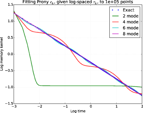
Figure 1: A least squares fit of the Prony mode coefficients $c_{k}$, $k\in\{1,\dots,N_{k}\}$, assuming log-spaced $\tau_{k}$, for each of $N_{k}$ modes. This fit is sufficient to illustrate the variance reduction achieved by the common random path coupling.

III.4 Integration scheme

We integrate the system using a modified Verlet method proposed by other authors, ensuring that the choice of method parameters satisfies the consistency condition and preserves the Langevin limit.Baczewski and Bond (2013) In many molecular dynamics simulations, the initial velocity $v_{0}$, and hence $s_{k,0}$, are chosen from a thermal distribution. In the numerical experiments below, the initial conditions for the particle position and velocity are taken to be definite and $s_{k,0}=0$ for all $k$. This is done to minimize the sources of the statistical error thus clarifying the reporting of deviations in the numerical results and the inclusion of thermal initial conditions does not pose a challenge to the method.

III.5 Normalized Autocorrelation Functions

The results of our numerical experiments are given primarily in term of normalized autocorrelation functions. Formally, the normalized $\operatorname{VACF}$ is given by

$$\overline{\operatorname{VACF}(t)}=\langle V_{t}V_{0}\rangle/\langle V_{0}V_{0}\rangle=\langle V_{t}\rangle/v_{0},$$ (19)

where the second equality holds when the initial velocity is definite. A similar definition is assigned to the normalized position autocorrelation function ($\operatorname{PACF}$). For the GLE with a harmonic confining potential and a power law memory kernel, expressions for the autocorrelation functions can be given in terms of Mittag-Leffler functions and their derivatives.Despósito and Vinales (2009) We compute the normalized $\operatorname{VACF}$ and $\operatorname{PACF}$ using the integrated velocity and position distributions and the fast Fourier transform method.Allen and Tildesley (1989) Figure 2 illustrates the $\overline{\operatorname{VACF}}$ for models with a varying number of Prony modes, i.e. extended variables, compared to an asymptotically exact quantity for the normalized $\operatorname{VACF}$ for the GLE.

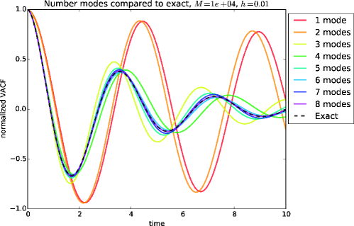
Figure 2: Small changes to the number of modes leads to qualitatively different behavior of the $\overline{\operatorname{VACF}}$ for the GLE with a harmonic confining potential.

IV Numerical experiments

The numerical experiments below focus on SA for extended variable GLE for one particle in one dimension with a power law memory kernel. The first experiment, in §IV.1, concerns the sensitivity with respect to the Prony coefficients $c_{k}$ where the coefficients are fit using the method described in §III.3. We observe that the reduction to the variance of the difference (8) for the optimally coupled dynamics is on the order of the bias squared for convex potentials.

IV.1 Sensitivity with respect to Prony coefficients

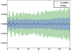
(a) $\mathcal{S}_{\varepsilon}(t,c_{1};\overline{\operatorname{VACF}})$, $M=10^{2}$

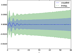
(b) $\mathcal{S}_{\varepsilon}(t,c_{1};\overline{\operatorname{VACF}})$, $M=10^{4}$

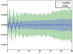
(c) $\mathcal{S}_{\varepsilon}(t,c_{3};\overline{\operatorname{VACF}})$, $M=10^{2}$

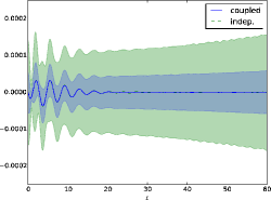
(d) $\mathcal{S}_{\varepsilon}(t,c_{3};\overline{\operatorname{VACF}})$, $M=10^{4}$

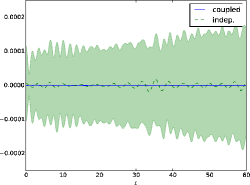
(e) $\mathcal{S}_{\varepsilon}(t,c_{6};\overline{\operatorname{VACF}})$, $M=10^{2}$

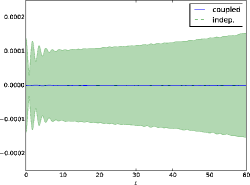
(f) $\mathcal{S}_{\varepsilon}(t,c_{6};\overline{\operatorname{VACF}})$, $M=10^{4}$

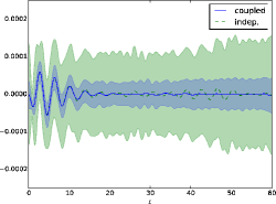
(g) $\mathcal{S}_{\varepsilon}(t,\omega;\overline{\operatorname{VACF}})$, $M=10^{2}$

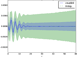
(h) $\mathcal{S}_{\varepsilon}(t,\omega;\overline{\operatorname{VACF}})$, $M=10^{4}$

Figure 3: The computational advantage of the common random path coupling is illustrated by the reduced sample size required to obtain meaningful estimates for sensitivities. Here we plot the sample mean with error bars denoting two standard deviations, based on $M=10^{2}$ samples (left column) and $M=10^{4}$ samples (right column), for various parameters.

We begin by computing local sensitivities for the proposed model with a harmonic confining potential. In particular, we investigate the sensitivity with respect to the Prony coefficients $c_{k}$ for $k\in\{1,\dots,N_{k}\}$, the harmonic potential frequency $\omega$, and the temperature $\mathsf{T}$, that is, for a set of parameters $\theta=(\omega,\mathsf{T},c_{1},\dots,c_{N_{k}})$. For the observable $\overline{\operatorname{VACF}(t)}=f(V_{t}^{\theta})$, the Monte Carlo finite difference estimator $\mathcal{S}_{\varepsilon}(t,\theta;\overline{\operatorname{VACF}})=\Delta_{c}(M,\varepsilon)$ based on the central difference is given by

$$\hat{\Delta}_{c}(M,\varepsilon)=\left(\hat{f}(V_{t}^{\theta_{i}+\varepsilon})-\hat{f}(V_{t}^{\theta_{i}-\varepsilon})\right)/2\varepsilon,$$

where $V_{t}^{\theta_{i}\pm\varepsilon}$ denotes a small $\varepsilon$ perturbation with respect to parameter $\theta_{i}$ leaving all other $\theta_{j}$, $j\neq k$, fixed. We compute $\hat{\Delta}_{c}$ for a bias $\varepsilon=0.01$ for dynamics that are driven by a common random path and that are driven by independent paths. In Figure 3, we compare the sample mean of estimators $\mathcal{S}_{\varepsilon}$, along with one standard deviation, for various parameters. The key observation here is that the optimal coupling dramatically reduces the variances of the difference estimator, relative to the independently sampled dynamics, even for a modestly sized sample.

The precise nature of the reduction can be deduced by varying $\varepsilon$ for a fixed index $\mathcal{S}_{\varepsilon}(t,\theta_{i};\overline{\operatorname{VACF}})$. In Figure 4, the variance of the difference (8) is compared for dynamics coupled with a common random path and independent dynamics for $\mathcal{S}_{\varepsilon}(t,c_{1};\overline{\operatorname{VACF}})$. For the optimally coupled dynamics, the reduction is $\operatorname{Var}[D(Z_{t})]=O(\varepsilon^{2})$, that is, on the order of the bias squared and, in contrast, $\operatorname{Var}[D(Z_{t})]=O(1)$ for the difference of the independent dynamics. Recalling the discussion of errors in §II.1, we see that for this example, $\operatorname{Var}[\hat{\Delta}_{c}]=O(M^{-1})$ in the case of the optimally coupled dynamics. That is, the optimal coupling eliminates the dependence of the variance of the estimator on the bias, asymptotically, in the case of a convex potential.

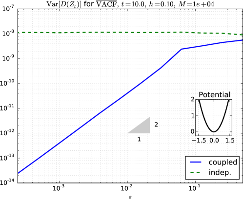
Figure 4: For $\mathcal{S}_{\varepsilon}(t=10,c_{1};\overline{\operatorname{VACF}})$ for an $N_{k}=8$ mode formulation of GLE, $\operatorname{Var}[D(Z_{t})]=O(\varepsilon^{2})$ for the common random path coupling in contrast to $\operatorname{Var}[D(Z_{t})]=O(1)$ for the naively sampled independent difference.

For nonlinear and non-convex potentials the common random path coupling reduces the variance of the estimator, although the rate is not expected to be $O(\varepsilon^{2})$. In Figure 5, the an $N_{k}=8$ mode formulation of GLE is considered with a simple double-well potential, $U(X_{t})=(1-X_{t}^{2})^{2}$, and $k_{B}\mathsf{T}=0.5$ for the sensitivities $\mathcal{S}_{\varepsilon}(t=10,c_{1};\overline{\operatorname{VACF}})$ and $\mathcal{S}_{\varepsilon}(t=10,c_{1};\overline{\operatorname{PACF}})$. In this setting, we observe a decay of less than $O(\sqrt{\varepsilon})$ for both observables. In particular, for the double well potential, the position time series, see Figure 6, indicates that the coupled dynamics can be pushed into distinct basins, increasing the covariance between the two paths.

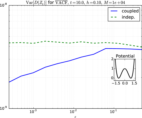
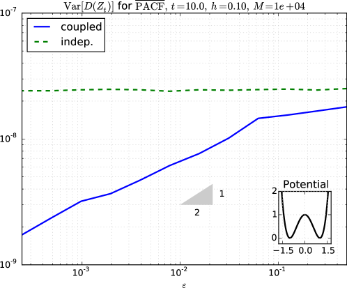
Figure 5: For simple nonlinear non-convex potentials, there is a net reduction to the variance from the common random path coupling. Here, for the double well potential, $U(X_{t})=(1-X_{t}^{2})^{2}$, with $k_{B}\mathsf{T}=0.5$, the reduction is less than $O(\sqrt{\varepsilon})$ for both the $\overline{\operatorname{PACF}}$ and $\overline{\operatorname{VACF}}$.

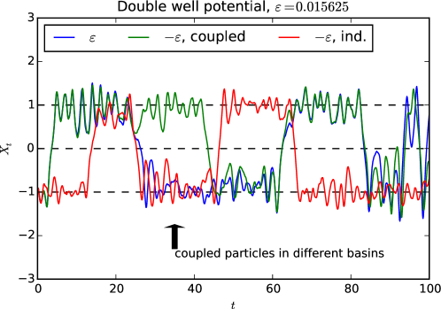
Figure 6: For nonlinear non-convex potentials, less substantial reductions to the variance are observed. For the double well potential, the coupled dynamics can be “pushed” into distinct basis resulting in a higher variance between the coupled paths.

For the extended variable GLE with a harmonic potential and a power law memory kernel, since analytical expressions exists for several observables of interest including the $\operatorname{VACF}$,Despósito and Vinales (2009) the maximum relative error for approximating the power law memory kernel with a given number of Prony modes can be computed a priori.Baczewski and Bond (2013) For more complicated potentials, exact expressions for observables and statistics of the dynamics are not available. Further, in reality one would like to fit the Prony modes to experimentally obtained data. Such a procedure would likely involve complex inference methods and a nonlinear fitting to obtain the $\tau_{k}$ and $c_{k}$. In such instances, it would be highly relevant to test the sensitivity of the fitted parameters.

IV.2 Sensitivity with respect to number of Prony modes

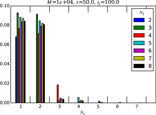
Figure 7: The non-local sensitivity $\mathcal{S}^{*}$ gives a quantitative characterization of the difference between the observed $\overline{\operatorname{VACF}}$ for models with different numbers of modes (c.f. Figure 2).

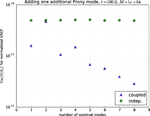
Figure 8: The common random path coupling is a valid tool for global SA, as illustrated by the reduced computational cost in computing $\operatorname{Var}[D(Z_{t})]$ where the difference is between a nominal model with a fixed number of Prony modes and an alternative model with one additional Prony mode. This difference, although it cannot be expressed as a derivative, provides a characterization of the sensitivity.

From Figure 2, we see that changing the number of Prony modes has a qualitative impact on the $\overline{\operatorname{VACF}}$. This motivates the numerical experiment that follows, where we analyze the effect of increasing the number of Prony modes. That is, for $N_{1}<N_{2}$ consider two systems with $N_{1}$ and $N_{2}$ extended variables, respectively. Given the difference $D(Z_{t})=f(V_{t}^{N_{1}})-f(V_{t}^{N_{2}})$, define a sensitivity

$$\mathcal{S}^{*}=\sum_{t}|\widehat{D(Z_{t})}|^{2}/\sigma_{Z_{t}},$$

where the carat denotes a sample mean, $\sigma_{Z_{t}}$ is the standard deviation of the associated sample mean $\widehat{D(Z_{t})}$, and the sum is over the space of discrete time points up to a fixed time $t<T$. Although this sensitivity is not a sensitivity in the sense of the gradients introduced previously, $\mathcal{S}^{*}$ gives a quantitative characterization of the difference between the two systems, see Figure 7.

The optimal coupling can be used to reduce the variance of such non-local perturbations. Here we investigate the difference between a nominal model with $N_{1}=n$, for $n=\{1,\dots,8\}$, and a perturbed model with one additional mode $N_{2}=N_{1}+1$. In Figure 8, we plot the variance of the difference generated by these nominal and perturbed dynamics for both the optimally coupled and independent cases, illustrating the reduced computational cost in sampling the optimally coupled dynamics in comparison to independent sampling. Here the Prony series are fit separately for the nominal and perturbed dynamics using the method outlined in §III.3. Auxiliary variables $c_{N_{1}+1}=0$ and $\tau_{N_{1}+1}=1$ are added to the nominal system so that the vectors for the nominal and perturbed dynamics have the same size, and then the common random path coupling is naively carried out for each of the components.

V Conclusions

We develop a general framework for variance reduction via coupling for goal-oriented SA for continuous time stochastic dynamics. This theory yields efficient Monte Carlo finite difference estimators for sensitivity indices that apply to all parameters of interest in an extended variable formulation of the GLE. Other well known SA techniques, such as likelihood ratio and pathwise methods are not applicable to key parameters of interest for this model. These estimators are obtained by coupling the nominal and perturbed dynamics appearing in the difference estimator through a common random path and are thus easy to implement. Strong heuristics are provided to demonstrate the optimality of the common random path coupling in this setting. In particular, for the extended variable GLE with convex potential, the reduction to the variance of the estimator is on the order of the bias squared, mitigating the effect of the bias error on the computational cost. Moreover, the common random path coupling is a valid computational tool in other aspects of UQ including non-local perturbations and finite difference estimators for global SA.

Appendix A Other examples of interest in particle dynamics

A.1 OU processes

OU processes are simple and easily analyzed yet are insightful as they posses several important features: the processes are Markovian, Gaussian, and stationary under the appropriate choice of initial conditions. Further, we note that the evolution of the extended variables in (17) is described by an OU process.

Consider the SDE

$$\mathrm{d}X_{t}=\theta(\mu-X_{t})\mathrm{d}t+\sigma\mathrm{d}W_{t},$$ (20)

subject to the initial condition $X_{t}=x_{0}\sim h$, for a given distribution $h$, with scalar coefficients $\theta,\sigma>0$, and $\mu\in\mathbf{R}$. Here $(W_{t})_{t\geq 0}$ is a Wiener process on a given stochastic basis. The solution to (20), given by

$$X_{t}=x_{0}e^{-\theta t}+\mu(1-e^{-\theta t})+\sigma e^{-\theta t}\int_{0}^{t}e^{\theta s}\mathrm{d}W_{s},$$ (21)

for $t\in[0,T]$, is the OU process. This process depends on parameters $\theta$, $\mu$, $\sigma$, $x_{0}$, and $h$.

As discussed in §II, we are interested in minimizing the variance of (8), where $(X^{1}_{t},X^{2}_{t})$ is given by the system

$$\begin{split}&\mathrm{d}X^{1}_{t}=\theta_{1}(\mu_{1}-X^{1}_{t})\mathrm{d}t+\sigma_{1}\mathrm{d}W^{1}_{t},\qquad X^{1}_{0}=x^{1}_{0}\sim h_{1}\\ &\mathrm{d}X^{2}_{t}=\theta_{2}(\mu_{2}-X^{2}_{t})\mathrm{d}t+\sigma_{2}\mathrm{d}W^{2}_{t},\qquad X^{2}_{0}=x^{2}_{0}\sim h_{2}.\end{split}$$ (22)

Then

$$\operatorname{Var}[D(Z_{t})] =\operatorname{Var}[f(X^{1}_{t})]+\operatorname{Var}[f(X^{2}_{t})]$$

$$\qquad+2\operatorname{\mathbf{E}}[f(X^{1}_{t})]\operatorname{\mathbf{E}}[f(X^{2}_{t})]$$

$$\qquad-2\operatorname{\mathbf{E}}[f(X^{1}_{t})f(X^{2}_{t})]$$

$$=\operatorname{Var}[f(X^{1}_{t})]+\operatorname{Var}[f(X^{2}_{t})]$$

$$\qquad-2\operatorname{Cov}[f(X^{1}_{t}),f(X^{2}_{t})],$$

and hence to minimize the variance of the difference we seek to maximize the covariance appearing in the expression above. If $X^{1}_{t}$ and $X^{2}_{t}$ are independent, that is, they are generated with independent processes $W^{1}$ and $W^{2}$, then the covariance in question will vanish. If we inject some dependence between $X^{1}$ and $X^{2}$ so that the covariance is nonzero, we find, after cancellation (for linear $f$), that the covariance is given by

$$\operatorname{\mathbf{E}}\left[f\left(\sigma_{1}e^{-\theta_{1}t}\int_{0}^{t}e^{\theta_{1}s}\mathrm{d}W_{s}\right)f\left(\sigma_{2}e^{-\theta_{2}t}\int_{0}^{t}e^{\theta_{2}s}\mathrm{d}W_{s}\right)\right].$$

This covariance is maximized when the stochastic integral processes above are dependent, which occurs when the driving processes $W^{1}$ and $W^{2}$ are assumed to be linearly dependent.

We shall look at two concrete observables, to gain intuition on the variance reduction introduced by the common random path coupling for the sensitivity with respect to different parameters. For simplicity, we shall further assume that $x_{0}^{1}=x_{0}^{2}$ and that $\mu_{1}=\mu_{2}$ are definite. Then these terms do not play a role since cancellations occur, for example, when $\operatorname{\mathbf{E}}[x_{0}]^{2}=\operatorname{\mathbf{E}}[x_{0}^{2}]$. In these examples, the coupling with a common random path reduces the variance in the computation of the central difference estimator by a factor $O(\varepsilon^{2})$ for the sensitivity with respect to $\theta$ and $\sigma$.

For both observable, and for the sensitivity with respect to $\theta$ and $\sigma$, we find that $\operatorname{Var}[D(Z_{t})]=O(\varepsilon^{2})$ when sampling coupled paths and $\operatorname{Var}[D(Z_{t})]=O(1)$ when sampling independent paths. Therefore, for standard first order difference estimators of the sensitivity indices, we have $\operatorname{Var}[\hat{\Delta}_{c}]=O(M^{-1})$, when sampling optimally coupled paths, but $\operatorname{Var}[\hat{\Delta}_{c}]=O(\varepsilon^{-2}M^{-1})$, for independently sampled paths. For the OU process, the optimal coupling eliminates the asymptotic dependence of the variance of the estimator on $\varepsilon$, in contrast to the case of sampling independent paths.

A.1.1 Finite time observable

Consider the finite time observable, $f(X_{t})=X_{T}$ for $T<\infty$. The expression for the covariance simplifies to

$$\operatorname{Cov}[ X^{1}_{T},X^{2}_{T}]$$

$$=\sigma_{1}\sigma_{2}e^{-(\theta_{1}+\theta_{2})T}\operatorname{\mathbf{E}}\left[\int_{0}^{T}e^{\theta_{1}u}\mathrm{d}W_{u}\int_{0}^{T}e^{\theta_{2}v}\mathrm{d}W_{v}\right]$$

$$=\sigma_{1}\sigma_{2}e^{-(\theta_{1}+\theta_{2})T}\int_{0}^{T}e^{(\theta_{1}+\theta_{2})s}\mathrm{d}s$$

$$=\sigma_{1}\sigma_{2}e^{-(\theta_{1}+\theta_{2})T}(e^{(\theta_{1}+\theta_{2})T}-1)/(\theta_{1}+\theta_{2})$$

$$=\sigma_{1}\sigma_{2}(1-e^{-(\theta_{1}+\theta_{2})T})/(\theta_{1}+\theta_{2}).$$

Thus the variance of the difference $D(Z_{t})$ converges to a constant, depending on $\varepsilon$, as $T\to\infty$. As the variance of the difference does not vanish, the coupling with a common random path is useful computational technique for all finite times.

Consider now the sensitivity with respect to $\theta$. Then $\theta_{1}(\theta,\varepsilon)$ and $\theta_{2}(\theta,\varepsilon)$ can be viewed as functions of $\theta$ and $\varepsilon$, i.e., $\theta_{1}=\theta+\varepsilon$ and $\theta_{2}=\theta-\varepsilon$ for the central difference. To determine the asymptotic dependence of $\operatorname{Var}[D(Z_{t})]$ on $\varepsilon$, we expand the variance of the difference in a series in $\varepsilon$ at zero. For standard first order differences (central, forward, and backward), in the case of independent sampling one finds

$$\operatorname{Var}[X^{1}_{T}]+\operatorname{Var}[X^{2}_{T}]=\sigma^{2}\theta^{-1}-\sigma^{2}\theta^{-1}e^{-2T\theta}+O(\varepsilon),$$

since $\theta_{1}(0)=\theta_{2}(0)=\theta$. That is, the variance of the difference is $O(1)$. In contrast, for sampling with common random paths, one finds

$$\operatorname{Var}[X^{1}_{T}]+\operatorname{Var}[X^{2}_{T}]-2\operatorname{Cov}[X^{1}_{T},X^{2}_{T}]=O(\varepsilon^{2}).$$

A similar story holds for the sensitivity with respect to $\sigma$: $\operatorname{Var}[D(Z_{t})]=O(1)$ for independent sampling and $\operatorname{Var}[D(Z_{t})]=O(\varepsilon^{2})$ for sampling with common random paths, when using standard first order differences.

A.1.2 Time average observable

Next we consider the time average observable defined by $\overline{X}=T^{-1}\int_{0}^{T}X_{s}\mathrm{d}s$. Once again, we wish to investigate the dependence of $\operatorname{Var}[D(Z_{t})]$ on $\varepsilon$ for the case of coupled paths and independent sampling. The expression for the covariance in this instance is

$$\operatorname{Cov}[\overline{X^{1}},\overline{X^{2}}] =\operatorname{\mathbf{E}}\left[T^{-1}\int_{0}^{T}\sigma_{1}e^{-\theta_{1}s}\int_{0}^{s}e^{\theta_{1}u}\mathrm{d}W_{u}\mathrm{d}s\;T^{-1}\int_{0}^{T}\sigma_{2}e^{-\theta_{2}t}\int_{0}^{t}e^{\theta_{2}v}\mathrm{d}W_{v}\mathrm{d}t\right]$$

$$=\sigma_{1}\sigma_{2}T^{-2}\int_{0}^{T}\int_{0}^{T}e^{-\theta_{1}s-\theta_{2}t}\operatorname{\mathbf{E}}\left[\int_{0}^{t}e^{\theta_{1}u}\mathrm{d}W_{u}\int_{0}^{s}e^{\theta_{2}v}\mathrm{d}W_{v}\right]\mathrm{d}s\mathrm{d}t$$

$$=\sigma_{1}\sigma_{2}T^{-2}\int_{0}^{T}\int_{0}^{T}e^{-\theta_{1}s-\theta_{2}t}\int_{0}^{s\wedge t}e^{(\theta_{1}+\theta_{2})r}\mathrm{d}r\mathrm{d}s\mathrm{d}t$$

$$=\sigma_{1}\sigma_{2}T^{-1}\left(\left(\theta_{1}\theta_{2}+\theta_{2}^{2}\right)^{-1}+\left(\theta_{1}^{2}+\theta_{1}\theta_{2}\right)^{-1}\right)+O(T^{-2}).$$

First we look at the sensitivity with respect to the parameter $\theta$. As in the case for the finite time observable, we expand $\operatorname{Var}[D(Z_{t})]$ in a series in $\varepsilon$ at zero. For standard first order differences this yields

$$\operatorname{Var}[D(Z_{t})] =2\sigma^{2}T^{-1}\theta^{-2}-3\sigma^{2}T^{-1}\theta^{-3}$$

$$+4\sigma^{2}T^{-2}\theta^{-3}e^{-T\theta}-\sigma^{2}T^{-2}\theta^{-3}e^{-2T\theta}+O(\varepsilon),$$

for independently sampled paths. Working in a similar fashion, we find in contrast that,

$$\operatorname{Var}[D(Z_{t})]=\varepsilon^{2}\left(4\sigma^{2}T^{-1}\theta^{-4}+O(T^{-2})\right)+O(\varepsilon^{4}),$$

for the coupled paths. For the sensitivity with respect to $\sigma$, the story is the same. The independently sampled paths behave like

$$\operatorname{Var}[D(Z_{t})]=2\sigma^{2}T^{-1}\theta^{-2}+\varepsilon^{2}2T^{-1}\theta^{-2}+O(T^{-2})\left(1+\varepsilon^{2}\right)$$

and the coupled paths behave like

$$\operatorname{Var}[D(Z_{t})]=\varepsilon^{2}\left(cT^{-1}\theta^{-2}+O(T^{-2})\right),$$

for a constant $c$.

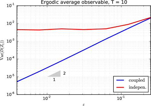
Figure 9: For the OU process, the variance of the estimator for the sensitivity with respect to $\sigma$ for the time averaged observable is $O(1)$ for the independently sampled difference and $O(\varepsilon^{2})$ for the optimally coupled difference. Here consider an OU process with parameters $\theta=1$, $\mu=1.2$, $\sigma=0.3$, and $x_{0}=2$ and compute the average up to time $T=10$. Each variance is based on $M=10^{3}$ independent samples of optimally coupled $\operatorname{AR}(1)$ processes and independent $\operatorname{AR}(1)$ processes.

In Figure 9, we observe the theoretically obtained values for the reduction to the variance for the sensitivity with respect to $\sigma$, of an OU process with parameters $\theta=1$, $\mu=1.2$, $\sigma=0.3$, and $x_{0}=2$. The time average average is computed up to time $T=10$ and each variance is computed using $M=10^{3}$ independent samples of an optimally coupled $\operatorname{AR}(1)$ processes and an independent $\operatorname{AR}(1)$ processes.

A.2 Langevin dynamics

We consider the LE with particle mass $m=1$,

$$\mathrm{d}X_{t}=V_{t}\mathrm{d}t,$$

$$\mathrm{d}V_{t}=-\omega^{2}X_{t}\mathrm{d}t-\beta V_{t}\mathrm{d}t+\sqrt{2\beta k_{B}\mathsf{T}}\mathrm{d}W^{1}_{t},$$

for $t\in[0,T]$, subject to $X_{0}=x_{0}$ and $V_{0}=v_{0}$, where $(W^{1}_{t})_{t\geq 0}$ is a Wiener process. This system can be written as a two-dimensional OU process $Y_{t}=(X_{t},V_{t})$, given by

$$\mathrm{d}Y_{t}=-BY_{t}\mathrm{d}t+\Sigma\mathrm{d}W_{t},\qquad Y_{0}=(x_{0},v_{0}),$$ (23)

for $W_{t}=(0,W^{1}_{t})$ with coefficient matrices

$$B=\begin{pmatrix}0&-1\\ \omega^{2}&\beta\end{pmatrix}\qquad\text{and}\qquad\Sigma=\begin{pmatrix}0&0\\ 0&\sqrt{2\beta k_{B}\mathsf{T}}\end{pmatrix}.$$

The general solution to (23) is given by

$$Y_{t}=e^{-Bt}Y_{0}+\int_{0}^{t}e^{-B(t-s)}\Sigma\mathrm{d}W_{s},$$ (24)

for $t\in[0,T]$, where, for this example, $e^{-Bt}$ can be written as (except in the critically damped case) in a closed form in terms of the eigenvalues of $B$: $\mu_{1}=\beta/2+\sqrt{\beta^{2}/4-\omega^{2}}$ and $\mu_{2}=\beta/2-\sqrt{\beta^{2}/4-\omega^{2}}$.Nelson (1967) That is, the position and velocity are given component-wise by

$$X_{t} =\mu^{-1}\Big{(}x_{0}(\mu_{1}e^{-\mu_{2}t}-\mu_{2}e^{-\mu_{1}t})+v_{0}(e^{-\mu_{2}t}-e^{-\mu_{1}t})$$

$$+\sqrt{\gamma(\mu_{1}+\mu_{2})}\int_{0}^{t}(e^{-\mu_{2}(t-s)}-e^{-\mu_{1}(t-s)})\mathrm{d}W_{s}\Big{)},$$

$$V_{t} =\mu^{-1}\Big{(}x_{0}\omega^{2}(e^{-\mu_{1}t}-e^{-\mu_{2}t})+v_{0}(\mu_{1}e^{-\mu_{1}t}-\mu_{2}e^{-\mu_{2}t})$$

$$+\sqrt{\gamma(\mu_{1}+\mu_{2})}\int_{0}^{t}(\mu_{1}e^{-\mu_{1}(t-s)}-\mu_{2}e^{-\mu_{2}(t-s)})\mathrm{d}W_{s}\Big{)},$$

for $\mu^{-1}=(\mu_{1}-\mu_{2})$ and $\gamma=2k_{B}\mathsf{T}$. We shall further assume, for simplicity, that both $x_{0}$ and $v_{0}$ are definite.

For the Langevin dynamics we form the coupled system $Z_{t}=(Y_{t},\tilde{Y}_{t})$ where $\tilde{Y}$ solves (23) for $\tilde{B}$ and $\tilde{\Sigma}$ depending upon perturbed parameters (also denoted with tildes in the sequel) and with an independent Wiener process $\tilde{W}$. Once again, we are interested in minimizing the variance of the difference $D(Z_{t})=f(Y_{t})-f(\tilde{Y}_{t})$, for linear observables $f$. Note that $D(Z_{t})$ is a vector quantity (i.e., $\operatorname{Var}[D(Z_{t})]$ is the variance-covariance matrix),

$$\operatorname{Var}[D(Z_{t})]=\operatorname{Var}[f(Y_{t})]-2\operatorname{Cov}[f(Y_{t}),f(\tilde{Y}_{t})]+\operatorname{Var}[f(\tilde{Y}_{t})]$$

for $f(Y_{t})=(f(X_{t}),f(V_{t}))$, where $\operatorname{Cov}[f(Y_{t}),f(\tilde{Y}_{t})]$ has components $\operatorname{Cov}[f(X_{t}),f(\tilde{X}_{t})]$, $\operatorname{Cov}[f(V_{t}),f(\tilde{V}_{t})]$, and cross terms $\frac{1}{2}(\operatorname{Cov}[f(V_{t}),f(\tilde{X}_{t})]+\operatorname{Cov}[f(X_{t}),f(\tilde{V}_{t})])$. This covariance is zero when $Y_{t}$ and $\tilde{Y}_{t}$ are independent and can be maximized when $Y_{t}$ and $\tilde{Y}_{t}$ are linearly dependent, which is equivalent to generating $Y_{t}$ and $\tilde{Y}_{t}$ using common random paths $W_{t}=\tilde{W}_{t}$. Next we investigate the asymptotic dependence of $\operatorname{Var}[D(Z_{t})]$ on $\varepsilon$ for two observables, related to a finite time horizon and a time average, for sensitivities with respect to $\beta$.

A.2.1 Finite time observable

Consider the finite time observable $f(Y_{t}):=Y_{T}$. Using the component wise expression above, the covariance term related to the positions can be expressed in terms of the eigenvalues of the drift matrices for the nominal and perturbed systems. That is, we let $\operatorname{Cov}[X_{T},\tilde{X}_{T}]=\phi(\mu_{1},\mu_{2},\tilde{\mu}_{1},\tilde{\mu}_{2})$ where

$$\phi(\mu_{1},\mu_{2},\tilde{\mu}_{1},\tilde{\mu}_{2})=\frac{\gamma\sqrt{(\mu_{1}+\mu_{2})(\tilde{\mu}_{1}+\tilde{\mu}_{2})}}{(\mu_{1}-\mu_{2})(\tilde{\mu}_{1}-\tilde{\mu}_{2})} \Big{(}\frac{1-e^{-(\mu_{1}+\tilde{\mu}_{1})T}}{\mu_{1}+\tilde{\mu}_{1}}-\frac{1-e^{-(\mu_{1}+\tilde{\mu}_{2})T}}{\mu_{1}+\tilde{\mu}_{2}}$$

$$-\frac{1-e^{-(\mu_{2}+\tilde{\mu}_{1})T}}{\mu_{2}+\tilde{\mu}_{1}}+\frac{1-e^{-(\mu_{2}+\tilde{\mu}_{2})T}}{\mu_{2}+\tilde{\mu}_{2}}\Big{)}.$$

Similar expressions can be given for the covariances related to the velocity and the cross terms. Here the eigenvalues of the nominal and perturbed systems are (linear) functions of $\epsilon$ (and $\beta$) that are related by the type of difference quotient chosen to approximate the sensitivity.

In the case of a centered difference, $\mu_{1}=\mu_{1}(\varepsilon)$ and $\mu_{2}=\mu_{2}(\varepsilon)$ are defined, in the obvious way, as $\mu_{1}(\varepsilon)=(\beta+\varepsilon)/2+\sqrt{(\beta+\varepsilon)^{2}/4-\omega^{2}}$ and $\mu_{2}(\varepsilon)=(\beta+\varepsilon)/2-\sqrt{(\beta+\varepsilon)^{2}/4-\omega^{2}}$ and hence $\tilde{\mu}_{1}=\mu_{1}(-\varepsilon)$ and $\tilde{\mu}_{2}=\mu_{2}(-\varepsilon)$. In this case, we can write $\operatorname{Var}[X_{T}]=\psi(\mu_{1}(\varepsilon),\mu_{2}(\varepsilon))$ and $\operatorname{Var}[\tilde{X}_{T}]=\psi(\mu_{1}(-\varepsilon),\mu_{2}(-\varepsilon))$ where we define $\psi(\mu_{1},\mu_{2})=\phi(\mu_{1},\mu_{2},\mu_{1},\mu_{2})$.

The asymptotic dependence of $\operatorname{Var}[D(Z_{t})]=\operatorname{Var}[X_{T}]+\operatorname{Var}[\tilde{X}_{T}]-2\operatorname{Cov}[X_{T},\tilde{X}_{T}]$ on $\varepsilon$ can now be obtained by expanding the quantity of interest in a series in $\varepsilon=0$, using the representations above. That is, for each terms appearing above we have

$$\operatorname{Var}[X_{T}]=\left.\psi\right|_{\varepsilon=0}+\left.\partial_{\varepsilon}\psi\right|_{\varepsilon=0}\varepsilon+\left.\partial^{2}_{\varepsilon}\psi\right|_{\varepsilon=0}\varepsilon^{2}+O(\varepsilon^{3}),$$

$$\operatorname{Var}[\tilde{X}_{T}]=\left.\psi\right|_{\varepsilon=0}-\left.\partial_{\varepsilon}\psi\right|_{\varepsilon=0}\varepsilon+\left.\partial^{2}_{\varepsilon}\psi\right|_{\varepsilon=0}\varepsilon^{2}+O(\varepsilon^{3}),$$

$$\operatorname{Cov}[X_{T},\tilde{X}_{T}]=\left.\phi\right|_{\varepsilon=0}+\left.\partial_{\varepsilon}\phi\right|_{\varepsilon=0}\varepsilon+\left.\partial^{2}_{\varepsilon}\phi\right|_{\varepsilon=0}\varepsilon^{2}+O(\varepsilon^{3}),$$

where $\partial^{k}_{\varepsilon}$ denotes the $k$th derivative with respect to $\varepsilon$. Noting that $\left.\psi\right|_{\varepsilon=0}$ is non-zero, it follows that $\operatorname{Var}[X_{T}-\tilde{X}_{T}]=O(1)$ for independently sampled paths. For the common random path coupling, the zeroth order term in the expansion for $\operatorname{Var}[D(Z_{t})]$ vanishes since $\left.\psi\right|_{\varepsilon=0}=\left.\phi\right|_{\varepsilon=0}$. In this particular case, the first order term, $\left.\partial_{\varepsilon}\phi\right|_{\varepsilon=0}=0$, also vanishes since $\partial_{\mu_{j}}\phi=\partial_{\tilde{\mu_{j}}}\phi$ and $\tilde{\mu}_{j}^{\prime}(0)=-\mu_{j}^{\prime}(0)$, for $j=1,2$. Finally, noting that since $\partial_{\mu_{j}}\phi$ is not symmetric in $\mu_{j},\tilde{\mu}_{j}$, the second order term in the expansion for $\operatorname{Var}[D(Z_{t})]$ does not vanish, yielding $\operatorname{Var}[D(Z_{t})]=O(\varepsilon^{2})$. Explicit expansions can also be calculated for other standard first order differences and for the other covariance terms with similar asymptotic rates observed, namely $O(\varepsilon^{2})$ for the common random path coupling and $O(1)$ for independently sampled paths.

A.2.2 Time average observable

Let $\overline{X}=T^{-1}\int_{0}^{T}X_{t}\mathrm{d}t$ and consider the time average observable $f(Y_{t})=(\overline{X},\overline{V})$. As in the case of the time average observable for the OU process, the expectation can be exchanged with the integral in time, yielding explicit expressions for the covariances as in §A.2.1. Investigations into the asymptotic dependence of $\operatorname{Var}[D(Z_{t})]$ yield $O(\varepsilon^{2})$ in the optimally coupled case and $O(1)$ in the independent case. These rates are observed experimentally in Figure 10 where we consider $\operatorname{Var}[D(Z_{t})]=(\varphi)_{ij}$ (i.e., $\varphi_{11}=\operatorname{Var}[\overline{X^{1}}-\overline{X^{2}}]$), based on $M=10^{3}$ samples, for a central difference perturbation in $\beta$, at $\beta=1$ (the underdamped case $\beta<2\omega$). The time averages are computed up to a final time $T=10$ for sample paths from Langevin dynamics, with fixed parameters $x_{0}=-1$, $v_{0}=-0.1$, $\omega=1$, $m=1$, and $\gamma=1$, integrated using the BAOAB methodLeimkuhler and Matthews (2015) with $\Delta t=10^{-3}$.

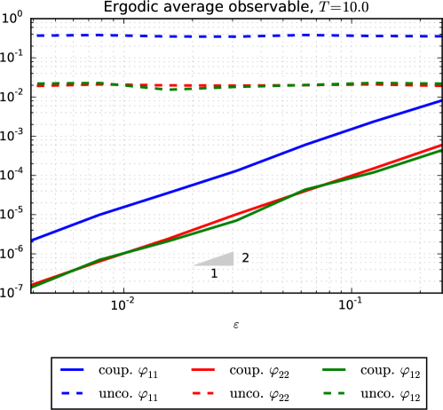
Figure 10: The sample variance of the components of $\operatorname{Var}[D(Z_{t})]$, for the time average observable $f(Z_{t})=\overline{Z}$, are on the order of $O(\varepsilon^{2})$ for optimally coupled paths, in contrast to $O(1)$ for independent paths. Here we consider of the sample variance of $\varphi_{11}$, $\varphi_{22}$, and $\varphi_{12}$, based on $M=10^{3}$ samples, for a central difference perturbation in $\beta$, at $\beta=1$, for time averages up to at $T=10$.

References

- Saltelli, Tarantola, and Campolongo (2000) A. Saltelli, S. Tarantola, and F. Campolongo, Statistical Science , 377 (2000).
- Saltelli et al. (2000) A. Saltelli, K. Chan, E. M. Scott, et al., Sensitivity analysis, Vol. 1 (Wiley New York, 2000).
- Coffey and Kalmykov (2012) W. T. Coffey and Y. P. Kalmykov, The Langevin Equation: With Applications to Stochastic Problems in Physics, Chemistry and Electrical Engineering, Vol. 27 (World Scientific, 2012).
- Baczewski and Bond (2013) A. D. Baczewski and S. D. Bond, J. Chem. Phys. 139, 044107 (2013).
- Mason and Weitz (1995) T. G. Mason and D. Weitz, Physical review letters 74, 1250 (1995).
- Goychuk (2012) I. Goychuk, Advances in Chemical Physics 150, 187 (2012).
- Lysy et al. (2016) M. Lysy, N. S. Pillai, D. B. Hill, M. G. Forest, J. W. Mellnik, P. A. Vasquez, and S. A. McKinley, Journal of the American Statistical Association , 00 (2016).
- Kantorovich (2008) L. Kantorovich, Physical Review B 78, 094304 (2008).
- Kantorovich and Rompotis (2008) L. Kantorovich and N. Rompotis, Physical Review B 78, 094305 (2008).
- Stella, Lorenz, and Kantorovich (2014) L. Stella, C. Lorenz, and L. Kantorovich, Physical Review B 89, 134303 (2014).
- Ness et al. (2015) H. Ness, L. Stella, C. Lorenz, and L. Kantorovich, Physical Review B 91, 014301 (2015).
- Ness et al. (2016) H. Ness, A. Genina, L. Stella, C. Lorenz, and L. Kantorovich, Physical Review B 93, 174303 (2016).
- Ceriotti, Manolopoulos, and Parrinello (2011) M. Ceriotti, D. E. Manolopoulos, and M. Parrinello, The Journal of chemical physics 134, 084104 (2011).
- Morrone et al. (2011) J. A. Morrone, T. E. Markland, M. Ceriotti, and B. Berne, The Journal of chemical physics 134, 014103 (2011).
- Ceriotti, Bussi, and Parrinello (2010) M. Ceriotti, G. Bussi, and M. Parrinello, Journal of Chemical Theory and Computation 6, 1170 (2010).
- Ceriotti et al. (2010) M. Ceriotti, M. Parrinello, T. E. Markland, and D. E. Manolopoulos, The Journal of chemical physics 133, 124104 (2010).
- Ceriotti, Bussi, and Parrinello (2009a) M. Ceriotti, G. Bussi, and M. Parrinello, Physical review letters 102, 020601 (2009a).
- Ceriotti, Bussi, and Parrinello (2009b) M. Ceriotti, G. Bussi, and M. Parrinello, Physical review letters 103, 030603 (2009b).
- Chorin and Stinis (2007) A. Chorin and P. Stinis, Communications in Applied Mathematics and Computational Science 1, 1 (2007).
- Hijón et al. (2010) C. Hijón, P. Español, E. Vanden-Eijnden, and R. Delgado-Buscalioni, Faraday discussions 144, 301 (2010).
- Darve, Solomon, and Kia (2009) E. Darve, J. Solomon, and A. Kia, Proceedings of the National Academy of Sciences 106, 10884 (2009).
- Li et al. (2015) Z. Li, X. Bian, X. Li, and G. E. Karniadakis, The Journal of chemical physics 143, 243128 (2015).
- Chen and Glasserman (2007) N. Chen and P. Glasserman, Stochastic Processes and their Applications 117, 1689 (2007).
- Pantazis and Katsoulakis (2013) Y. Pantazis and M. A. Katsoulakis, The Journal of chemical physics 138, 054115 (2013).
- Glynn (1990) P. W. Glynn, Communications of the ACM 33, 75 (1990).
- Arampatzis, Katsoulakis, and Rey-Bellet (2016) G. Arampatzis, M. A. Katsoulakis, and L. Rey-Bellet, J. Chem. Phys. 144, 104107 (2016), 10.1063/1.4943388 .
- Fournié et al. (1999) E. Fournié, J.-M. Lasry, J. Lebuchoux, P.-L. Lions, and N. Touzi, Finance Stoch. 3, 391 (1999).
- Fournié et al. (2001) E. Fournié, J.-M. Lasry, J. Lebuchoux, and P.-L. Lions, Finance Stoch. 5, 201 (2001).
- Nualart (2006) D. Nualart, The Malliavin calculus and related topics, 2nd ed., Probability and its Applications (New York) (Springer-Verlag, Berlin, 2006) pp. xiv+382.
- Bouchard, Ekeland, and Touzi (2004) B. Bouchard, I. Ekeland, and N. Touzi, Finance Stoch. 8, 45 (2004).
- Warren and Allen (2012) P. B. Warren and R. J. Allen, Physical review letters 109, 250601 (2012).
- Assaraf et al. (2015) R. Assaraf, B. Jourdain, T. Lelièvre, and R. Roux, arXiv preprint arXiv:1509.01348 (2015).
- Ciccotti and Jacucci (1975) G. Ciccotti and G. Jacucci, Physical Review Letters 35, 789 (1975).
- Stoddard and Ford (1973) S. D. Stoddard and J. Ford, Physical Review A 8, 1504 (1973).
- Hairer and Majda (2010) M. Hairer and A. J. Majda, Nonlinearity 23, 909 (2010).
- Anderson (2012) D. F. Anderson, SIAM J. Numer. Anal. 50, 2237 (2012).
- Srivastava, Anderson, and Rawlings (2013) R. Srivastava, D. F. Anderson, and J. B. Rawlings, The Journal of chemical physics 138, 074110 (2013).
- Wolf and Anderson (2015) E. S. Wolf and D. F. Anderson, The Journal of chemical physics 142, 034103 (2015).
- Rathinam, Sheppard, and Khammash (2010) M. Rathinam, P. W. Sheppard, and M. Khammash, The Journal of chemical physics 132, 034103 (2010).
- Arampatzis and Katsoulakis (2014) G. Arampatzis and M. A. Katsoulakis, The Journal of chemical physics 140, 124108 (2014).
- Arampatzis, Katsoulakis, and Pantazis (2015a) G. Arampatzis, M. A. Katsoulakis, and Y. Pantazis, PloS one 10, e0130825 (2015a).
- Sheppard, Rathinam, and Khammash (2013) P. W. Sheppard, M. Rathinam, and M. Khammash, Bioinformatics 29, 140 (2013).
- Pantazis, Katsoulakis, and Vlachos (2013) Y. Pantazis, M. A. Katsoulakis, and D. G. Vlachos, BMC bioinformatics 14, 1 (2013).
- Tsourtis et al. (2015) A. Tsourtis, Y. Pantazis, M. A. Katsoulakis, and V. Harmandaris, The Journal of chemical physics 143, 014116 (2015).
- Arampatzis, Katsoulakis, and Pantazis (2015b) G. Arampatzis, M. A. Katsoulakis, and Y. Pantazis, in Stochastic Equations for Complex Systems (Springer, 2015) pp. 105–124.
- Dupuis et al. (2015) P. Dupuis, M. A. Katsoulakis, Y. Pantazis, and P. Plechac, arXiv preprint arXiv:1503.05136 (2015).
- Arampatzis, Katsoulakis, and Rey-Bellet (2015) G. Arampatzis, M. Katsoulakis, and L. Rey-Bellet, final published version? (2015).
- Morris (1991) M. D. Morris, Technometrics 33, 161 (1991).
- Campolongo, Cariboni, and Saltelli (2007) F. Campolongo, J. Cariboni, and A. Saltelli, Environmental modelling & software 22, 1509 (2007).
- Saltelli et al. (2008) A. Saltelli, M. Ratto, T. Andres, F. Campolongo, J. Cariboni, D. Gatelli, M. Saisana, and S. Tarantola, Global sensitivity analysis: the primer (John Wiley & Sons, 2008).
- Glasserman (2003) P. Glasserman, Monte Carlo methods in financial engineering, Vol. 53 (Springer Science & Business Media, 2003).
- L’Ecuyer and Perron (1994) P. L’Ecuyer and G. Perron, Operations Research 42, 643 (1994).
- L’Ecuyer (1992) P. L’Ecuyer, Annals of Operations Research 39, 121 (1992).
- Ikeda and Watanabe (1989) N. Ikeda and S. Watanabe, Stochastic differential equations and diffusion processes, 2nd ed., North-Holland Mathematical Library, Vol. 24 (North-Holland Publishing Co., Amsterdam, 1989) pp. xvi+555.
- Øksendal (2003) B. Øksendal, Stochastic differential equations, sixth ed., Universitext (Springer-Verlag, Berlin, 2003) pp. xxiv+360, an introduction with applications.
- Ben Hammouda, Moraes, and Tempone (2016) C. Ben Hammouda, A. Moraes, and R. Tempone, Numerical Algorithms , 1 (2016).
- Zwanzig (2001) R. Zwanzig, Nonequilibrium statistical mechanics (Oxford University Press, USA, 2001).
- Didier et al. (2012) G. Didier, S. A. McKinley, D. B. Hill, and J. Fricks, Journal of Time Series Analysis 33, 724 (2012).
- Rey-Bellet (2006) L. Rey-Bellet, in Open Quantum Systems II (Springer, 2006) pp. 41–78.
- Beylkin and Monzón (2005) G. Beylkin and L. Monzón, Applied and Computational Harmonic Analysis 19, 17 (2005).
- Beylkin and Monzón (2010) G. Beylkin and L. Monzón, Applied and Computational Harmonic Analysis 28, 131 (2010).
- Kunis et al. (2016) S. Kunis, T. Peter, T. Römer, and U. von der Ohe, Linear Algebra and its Applications 490, 31 (2016).
- Potts and Tasche (2010) D. Potts and M. Tasche, Signal Processing 90, 1631 (2010).
- Despósito and Vinales (2009) M. Despósito and A. Vinales, Physical Review E 80, 021111 (2009).
- Kou and Xie (2004) S. Kou and X. S. Xie, Physical review letters 93, 180603 (2004).
- Viñales and Despósito (2006) A. Viñales and M. Despósito, Physical Review E 73, 016111 (2006).
- Ottobre and Pavliotis (2011) M. Ottobre and G. Pavliotis, Nonlinearity 24, 1629 (2011).
- Allen and Tildesley (1989) M. P. Allen and D. J. Tildesley, Computer simulation of liquids (Oxford university press, 1989).
- Nelson (1967) E. Nelson, Dynamical Theories of Brownian Motion, second ed. ed. (Princeton University Press, Princeton, N.J., 1967) pp. iii+142.
- Leimkuhler and Matthews (2015) B. Leimkuhler and C. Matthews, Molecular Dynamics: With Deterministic and Stochastic Numerical Methods, Vol. 39 (Springer, 2015).