A lower bound on the spectrum of unimodular networks

Abstract.

Unimodular networks are a generalization of finite graphs in a stochastic sense. We prove a lower bound to the spectral radius of the adjacency operator and of the Markov operator of an unimodular network in terms of its average degree. This allows to prove an Alon-Boppana type bound for the largest eigenvalues in absolute value of large, connected, bounded degree graphs, which generalizes the Alon-Boppana theorem for regular graphs.

A key step is establishing a lower bound to the spectral radius of an unimodular tree in terms of its average degree. Similarly, we provide a lower bound on the volume growth rate of an unimodular tree in terms of its average degree.

1. Introduction

The Alon-Boppana theorem [14] states that if $G_{n}$ is a sequence of finite, connected, $d$-regular graphs with $|G_{n}|\to\infty$ then the second largest eigenvalue of the adjacency matrix of $G_{n}$ in absolute value, say $\sigma_{2}(G_{n})$, satisfies $\liminf_{n}\,\sigma_{2}(G_{n})\geq 2\sqrt{d-1}$. The quantity $2\sqrt{d-1}$ is the spectral radius of the $d$-regular tree, which represents the exponential growth rate of the number of closed walks in the $d$-regular tree around a fixed vertex. Another version of the theorem by Serre [15] states that for any $\epsilon>0$, there is a positive constant $c(\epsilon,d)$ such that any finite $d$-regular graph has at least $c(\epsilon,d)$-proportion of its eigenvalues having absolute value larger than $2\sqrt{d-1}-\epsilon$.

What can be said about these types of spectral lower bounds for non-regular or even infinite graphs? This paper provides such bounds for unimodular networks, a generalization of finite graphs to a stochastic setting. Using the framework of local convergence of graphs this provides lower bounds to the top eigenvalues in absolute value of finite, bounded degree graphs in terms of their average degree. Before stating these results we explain some of the background.

Greenberg [9] extended the aforementioned theorem of Serre to arbitrary finite graphs, proving the following. Let $G$ be a locally finite, connected graph with a countable number of vertices. Let $W_{k}(G,x)$ be the set of closed walks in $G$ of length $k$ starting from a vertex $x$. Its spectral radius $\rho(G)$ is the operator norm of the adjacency matrix of $G$ acting on $\ell^{2}(G)$. Greenberg proved that for any tree $T$ and any $\epsilon>0$, there is a constant $c(\epsilon,T)>0$ such that if a finite graph $G$ has universal cover $T$ then at least $c(\epsilon,T)$-proportion of its eigenvalues have absolute value at least $\rho(T)-\epsilon$. (See [12] where the result is stated as well.) Various strengthenings of the Alon-Boppana theorem have later been proved in [6, 13], and [8] gives a Cheeger bound for graph Laplacians.

Afterwards, Hoory [10] proved that if $G$ is a finite graph with $m$ edges that is not a tree, and $T$ is its universal cover, then $\rho(T)\geq 2\sqrt{\Lambda}$ where $\Lambda=\prod_{v\in G}(\deg(v)-1)^{\deg(v)/2m}$. It can be shown that $\Lambda\geq d_{\mathrm{av}}(G)-1$, where $d_{\mathrm{av}}(G)$ is the average degree of $G$. Combining Greenberg’s theorem with Hoory’s implies that the set of finite and connected graphs sharing a common universal cover $T$ has the property that for any $\epsilon>0$, any graph $G$ from this set has at least $c(\epsilon,T)|G|$ eigenvalues with absolute value at least $2\sqrt{d_{\mathrm{av}}(G)-1}-\epsilon$.

Sharing a common universal cover is a form of spatial homogeneity for graphs. Indeed, if two finite graphs have a common universal cover then they also have a common finite cover [11]. This implies, for instance, that both graphs have the same spectral radius, average degree, and also the same degree distribution. In order to prove Alon-Boppana type bounds it is necessary to have some form of spatial homogeneity. As an example, if the complete graph on $n$-vertices is glued to a path of length $n$ at a common vertex then the average degree of the resulting graph is at least $n/2$ while all but the largest eigenvalues have absolute value at most 2.

We consider a stochastic form of spatial homogeneity whereby graphs look homogenous around most vertices. This is the notion of unimodular networks. Roughly speaking, a unimodular network is a random rooted graph, possibly infinite, that is homogeneous in the sense that shifting the root to its neighbour does not change the distribution; Section 1.1 contains the definition. Finite connected graphs with a uniform random choice of root are unimodular. Several examples and a rather thorough discussion about unimodular networks may also be found in [2] and references therein.

Under natural assumptions, we prove the spectral radius of a unimodular network is at least $2\sqrt{d_{\mathrm{av}}-1}$, where $d_{\mathrm{av}}$ is the expected degree of the root. A similar lower bound is proved for the spectral radius of its simple random walk, which seems to be new even for large finite graphs. As a consequence of these bounds one finds an analogue of Serre’s theorem for the adjacency and Markov operators of unimodular networks.

We also derive Alon-Boppana type bounds for the eigenvalues of the adjacency matrix and of the simple random walk (Markov operator) for any growing sequence of connected, bounded degree graphs. Regarding the adjacency matrix, suppose $G_{n}$ is a sequence of finite, connected, bounded degree graphs with size $|G_{n}|\to\infty$. Then the $j$-th largest eigenvalue of $G_{n}$ in absolute value, say $\sigma_{j}(G_{n})$, satisfies $\liminf_{n}\,\sigma_{j}(G_{n})\geq\liminf_{n}\,2\sqrt{d_{\mathrm{av}}(G_{n})-1}$. We also prove that the volume growth rate of a unimodular tree with no leaves is at least $d_{\mathrm{av}}-1$, where $d_{\mathrm{av}}$ is the expected degree of the root. This in turn provides a lower bound on the growth rate of non-backtracking walks in certain unimodular networks.

1.1. Unimodular network and mass transport principle

Let $(G,x)$ be a rooted graph where the distinguished vertex $x$ is the root, $G$ is locally finite, has a countable number of vertices and is connected. Two such rooted graphs are isomorphic if there is a graph isomorphism between them that takes the root of one graph to the other’s. Let $\mathcal{G}^{*}$ be the set of isomorphism classes of such rooted graphs. The distance between $(G,x),(H,y)\in\mathcal{G}^{*}$ may be defined as $1/(1+R)$, where $R=\min\{r:B_{r}(G,x)\cong B_{r}(H,y)\}$ and $B_{r}(G,x)$ is the $r$-neighbourhood of $x$ in $G$. With this distance, $\mathcal{G}^{*}$ is a Polish space. A random rooted graph is a Borel probability measure on $\mathcal{G}^{*}$, which is conveniently realized as a $\mathcal{G}^{*}$-valued random variable.

A random rooted graph $(G,\circ)$ is a unimodular network if

(1.1) $$\mathbf{E}\left[\sum_{x\in V(G)}f(G,\circ,x)\right]=\mathbf{E}\left[\sum_{x\in V(G)}f(G,x,\circ)\right]$$

for every non-negative and measurable function $f$ defined on the set of isomorphism classes of doubly rooted graphs $(G,x,y)$. Equation (1.1) is called the mass transport principle. To verify unimodularity it suffices that the mass transport principle holds only for those $f$ that satisfy $f(G,x,y)=0$ if $x$ and $y$ are not neighbours in $G$; see [2, Proposition 2.2].

Examples.

A finite graph $G$ rooted at a uniformly random vertex $\circ$ of $G$ is a unimodular network. The Cayley graph of any finitely generated group, rooted at its identity, is a deterministic unimodular network. So the lattices $\mathbb{Z},\mathbb{Z}^{2},\ldots$ are unimodular networks, as are the infinite regular trees $\mathbb{T}_{3},\mathbb{T}_{4}$, etc. Examples of unimodular trees include periodic trees, Poisson-Galton-Watson trees, and more generally, unimodular Galton-Watson trees [2, Examples 1.1 and 10.2].

Local convergence.

The space of random rooted graphs carries the topology of weak convergence: $(G_{n},\circ_{n})$ converges to $(G,\circ)$ if

$$\mathbf{E}\left[f(G_{n},\circ_{n})\right]\to\mathbf{E}\left[f((G,\circ))\right]$$

for every bounded and continuous $f:\mathcal{G}^{*}\to\mathbb{R}$. Restricted to unimodular networks, this provides the natural notion of convergence. The limit of a sequence of unimodular networks is also a unimodular network; see [5, Lemma 2.1]. This notion of convergence of unimodular networks, especially for finite graphs rooted uniformly at random, is called local convergence or also Benjamini-Schramm convergence as they formulated the concept [4].

As an example, the sequence of $n\times n$ tori as shown in Figure 1, each rooted at an uniformly random vertex, converges to the infinite grid $\mathbb{Z}^{2}$ rooted at its origin. The aforementioned unimodular Galton-Watson trees are local limits of random graphs with a given degree sequence.

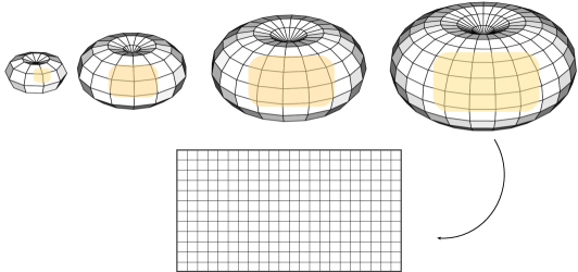
Figure 1. Growing discrete tori converge locally to the infinite grid $\mathbb{Z}^{2}$.

Spectral radius.

Recall that $W_{k}(G,x)$ is the set of closed walks in $G$ of length $k$ starting from $x$. The spectral radius of a unimodular network $(G,\circ)$ is defined to be

$$\rho(G)=\lim_{k\to\infty}\,\mathbf{E}\left[\,|W_{2k}(G,\circ)|\,\right]^{\frac{1}{2k}}.$$

The quantity $\mathbf{E}\left[|W_{k}(G,\circ)|\right]$ is in fact the $k$-th moment of a Borel probability measure of $\mathbb{R}$ called the spectral measure of $(G,\circ)$, as explained further in Section 2. The spectral radius is then the largest element in absolute value in the support of the spectral measure. If $G$ is a finite graph then its spectral measure is the empirical measure of the eigenvalues of its adjacency matrix.

Similarly, we can define the spectral measure and spectral radius of the simple random walk (SRW) on $(G,\circ)$. For $(G,x)\in\mathcal{G}^{*}$, let $p_{k}(G,x)$ be the $k$-step return probability of the SRW on $(G,x)$ started from vertex $x$. The spectral radius of the SRW on a unimodular network $(G,\circ)$ is

$$\rho_{\mathrm{SRW}}(G)=\lim_{k\to\infty}\,\mathbf{E}\left[p_{2k}(G,\circ)\right]^{\frac{1}{2k}}.$$

Universal cover.

The universal cover $T_{G}$ of a connected, locally finite graph $G$ is the unique tree for which there is a surjective graph homomorphism $\pi:T_{G}\to G$, called cover map, such that $\pi$ is an isomorphism on the 1-neighbourhood of every vertex. For $(G,x)\in\mathcal{G}^{*}$, let $(T_{G},\hat{x})$ be its universal cover rooted at any $\hat{x}$ such that $\pi(\hat{x})=x$ (all such $(T_{G},\hat{x})$ have the same rooted isomorphism class). The cover map sends closed walks in $T_{G}$ starting from $\hat{x}$ to closed walks in $G$ from $x$ in an injective manner. Thus, $\rho(G)\geq\rho(T_{G})$. The SRW on $(G,x)$ is the projection of the SRW on $(T_{G},\hat{x})$ by the cover map. Therefore, $\rho_{\mathrm{SRW}}(G)\geq\rho_{\mathrm{SRW}}(T_{G})$. If $(G,\circ)$ is a unimodular network then its universal cover tree $(T_{G},\hat{\circ})$ is also unimodular. Here, $(T_{G},\hat{\circ})$ is constructed for every sample outcome of $(G,\circ)$.

1.2. Statement of results

Theorem 1.

Let $(T,\circ)$ be a unimodular tree with $\mathbf{E}\left[\mathrm{deg}(\circ)\right]<\infty$ and no leaves almost surely. Then

$$\rho(T)\geq 2\,\exp{\left\{\frac{\mathbf{E}\left[\mathrm{deg}(\circ)\log(\sqrt{\mathrm{deg}(\circ)-1})\right]}{\mathbf{E}\left[\mathrm{deg}(\circ)\right]}\right\}}\geq 2\sqrt{\mathbf{E}\left[\mathrm{deg}(\circ)\right]-1}\,.$$

Additionally, if $(T,\circ)$ has deterministically bounded degree then

$$\rho_{\mathrm{SRW}}(T)\geq 2\,\exp{\left\{\frac{\mathbf{E}\left[\mathrm{deg}(\circ)\log\Big{(}\frac{\sqrt{\mathrm{deg}(\circ)-1}}{\mathrm{deg}(\circ)}\Big{)}\right]}{\mathbf{E}\left[\mathrm{deg}(\circ)\right]}\right\}}\geq\frac{2\,\mathbf{E}\left[\mathrm{deg}(\circ)\right]\sqrt{\mathbf{E}\left[\mathrm{deg}(\circ)\right]-1}}{\mathbf{E}\left[\mathrm{deg}(\circ)^{2}\right]}.$$

The following theorem is about the spectrum of the adjacency operator of unimodular networks and finite graphs.

Theorem 2.

I) Unimodular networks: Let $(G_{n},\circ)$ be a sequence of unimodular networks such that $(G_{n},\circ)\to(G,\circ)$ locally. Suppose that $\rho(G)<\infty$. Let $(T_{G},\circ)$ be the universal cover of $(G,\circ)$. Let $\mu_{n}$ denote the spectral measure of $(G_{n},\circ)$ and let $\mu_{T_{G}}$ denote it for $(T_{G},\circ)$.

For every $\epsilon>0$, there is a constant $c(\epsilon,\rho(G),\rho(T_{G}))>0$ such that

$$\liminf_{n\to\infty}\,\mu_{n}\left(\{|x|>\rho(T_{G})-\epsilon\}\right)\geq c(\epsilon,\rho(G),\rho(T_{G})).$$

II) Finite graphs: Let $G_{n}$ be a sequence of finite, connected graphs with vertex degrees bounded by $\Delta$ and $|G_{n}|\to\infty$. Let $\sigma_{j}(G_{n})$ be the $j$-th largest eigenvalue in absolute value of the adjacency matrix of $G_{n}$, counted with multiplicity; these are the singular values of $G_{n}$. Let $d_{\mathrm{av}}(G_{n})$ denote the average degree of $G_{n}$.

For every $j\geq 1$,

$$\liminf_{n\to\infty}\,\sigma_{j}(G_{n})\geq\liminf_{n\to\infty}\,2\sqrt{d_{\mathrm{av}}(G_{n})-1}\,.$$

The next theorem is about the spectrum of simple random walk. For a finite and connected graph $G$, its 2-core, denoted $G^{\mathrm{core}}$, is the subgraph obtained by iteratively removing leaves from $G$ until none remains. So if $G$ has no leaves then $G^{\mathrm{core}}$ equals $G$, whereas if $G$ is a tree then $G^{\mathrm{core}}$ is empty.

Theorem 3.

Let $G_{n}$ be a sequence of finite and connected graphs with all vertex degrees at most $\Delta$. Let $\mu^{\mathrm{SRW}}_{G_{n}}$ denote the empirical measure of the eigenvalues of the Markov operator of $G_{n}$, that is, of the matrix $P$ with entries $P(x,y)=\frac{1}{\deg{x}}\mathbf{1}_{\{x\sim y\}}$ for $x,y\in V(G_{n})$.

Suppose $|G_{n}|\to\infty$ and $|G_{n}^{\mathrm{core}}|/|G_{n}|\to 1$. Then for every $\epsilon>0$,

$$\liminf_{n\to\infty}\,\mu^{\mathrm{SRW}}_{G_{n}}\left(\left\{|x|>\frac{2\sqrt{d_{\rm{av}}(G_{n})-1}}{\frac{1}{2|E(G_{n})|}\sum_{x\in G_{n}}(\deg{x})^{2}}-\epsilon\right\}\right)>0.$$

Note that $\frac{1}{2|E(G_{n})|}\sum_{x\in G}(\deg{x})^{2}$ is the average degree of $G$ with respect to the stationary measure of its simple random walk, which assigns probability $\frac{\deg{x}}{2|E(G)|}$ to a vertex $x$.

The final theorem is about volume growth.

Theorem 4.

Let $(T,\circ)$ be a unimodular tree with $\mathbf{E}\left[\mathrm{deg}(\circ)\right]<\infty$ and with no leaves almost surely. Let $S_{r}(T,\circ)=\{x\in V(T):\mathrm{dist}_{T}(o,x)=r\}$. Then,

$$\mathbf{E}\left[|S_{r}(T,\circ)|\right] \geq\mathbf{E}\left[\mathrm{deg}(\circ)\right]\cdot\exp\left\{(r-1)\frac{\mathbf{E}\left[\mathrm{deg}(\circ)\,\log(\mathrm{deg}(\circ)-1)\right]}{\mathbf{E}\left[\mathrm{deg}(\circ)\right]}\right\}$$

$$\geq\mathbf{E}\left[\mathrm{deg}(\circ)\right](\mathbf{E}\left[\mathrm{deg}(\circ)\right]-1)^{r-1}.$$

The lower bound of $\mathbf{E}\left[\mathrm{deg}(\circ)\right](\mathbf{E}\left[\mathrm{deg}(\circ)\right]-1)^{r-1}$ follows from Jensen’s inequality applied to the convex function $x\log(x-1)$ for $x\geq 2$. Here is a consequence of Theorem 4; see [3] for a related result on finite graphs. Let $(G,\circ)$ be a unimodular network with no leaves almost surely and $\mathbf{E}\left[\mathrm{deg}(\circ)\right]<\infty$. Let $NBW_{r}(G,\circ)$ be the set of non-backtracking walks of length $r$ from the root. Then $NBW_{r}(G,\circ)$ is in bijection with $S_{r}(T_{G},\circ)$, hence,

(1.2) $$\mathbf{E}\left[|NBW_{r}(G,\circ)|\right]\geq\mathbf{E}\left[\mathrm{deg}(\circ)\right](\mathbf{E}\left[\mathrm{deg}(\circ)\right]-1)^{r-1}.$$

1.3. Outline of the paper

In Section 2 we discuss some concepts used in the proofs. Theorem 1 is proved in Section 3. Theorems 2 and 3 and 4 are proved in Section 4. The idea behind the proof of Theorem 1 is borrowed from Hoory [10]. It is based on counting walks in a unimodular tree according to their height function.

Acknowledgements

I thank Miklós Abért and Péter Csikvári for helpful comments. The research was partially supported by an NSERC PDF award.

2. Preliminaries

2.1. Spectrum of a unimodular network

For a unimodular network $(G,\circ)$ the quantity $\mathbf{E}\left[|W_{k}(G,\circ)|\right]$ is the $k$-th moment of a Borel probability measure $\mu_{G}$ on $\mathbb{R}$, called its spectral measure. Usually, the theory of von Neumann Algebras is used to define $\mu_{G}$ is general (see [5, Section 2.3] or [2, Section 5]). One has that

$$\mu_{G}(B)=\mathbb{E}_{(G,\circ)}\left[\mu^{\delta_{\circ}}_{A_{G}}(B)\right],$$

where $\mu^{\delta_{\circ}}_{A_{G}}$ is the spectral measure at the function $\delta_{\circ}$ of the adjacency operator of $G$ acting on $\ell^{2}(G)$.

The spectral radius of $(G,\circ)$ can also be formulated in terms of the spectral measure: $\rho(G)=\sup\,\{|x|:x\in\mathrm{support}(\mu_{G})\}.$ The spectral measure $\mu^{\mathrm{SRW}}_{G}$ and spectral radius $\rho_{\mathrm{SRW}}(G)$ of the SRW on $(G,\circ)$ are defined similarly with respect to the Markov operator acting on $\ell^{2}(G)$. The probability measure $\mu^{\mathrm{SRW}}_{G}$ is supported inside the interval $[-1,1]$; thus, $\rho_{\mathrm{SRW}}(G)\leq 1$. Moreover, its moments are

$$\int x^{k}\,d\mu^{\mathrm{SRW}}_{G}=\mathbf{E}\left[p_{k}(G,\circ)\right].$$

If a sequence of unimodular networks $(G_{n},\circ)$ converges to $(G,\circ)$ locally then their spectral measures $\mu_{G_{n}}$ converge to $\mu_{G}$ weakly [5, Proposition 2.2]. Similarly, $\mu^{\mathrm{SRW}}_{G_{n}}\to\mu^{\mathrm{SRW}}_{G}$ weakly.

2.2. Edge rooted graphs and non-backtracking walk

The non-backtracking walk (NBW) is a Markov process on the space of directed, edge rooted graphs with no leaves. It does exactly as it sounds as shown by Figure 2.

Define $\mathcal{G}^{**}$ to be set of isomorphism classes of doubly rooted graphs $(G,x,y)$ analogous to $\mathcal{G}^{*}$. Now for $(G,x,y)\in\mathcal{G}^{**}$ with $(x,y)\in E(G)$, let $e=(x,y),e^{-}=x,e^{+}=y$ and $\overset{\shortleftarrow}{e}=(y,x)$. One step of the non-backtracking walk gives a random element $(G,e^{+},z)\in\mathcal{G}^{**}$, where $z$ is a uniform random neighbor of $e^{+}$ that is different from $e^{-}$. Let $\mathrm{NBW}(G,e)$ denote the outcome of one step of the NBW starting from $(G,e)=(G,x,y)$. Thus,

$$\mathbf{Pr}\left[\mathrm{NBW}(G,e)=(H,f)\right]=\begin{cases}\frac{1}{\deg(e^{+})-1}&\text{if}\;(H,f)=(G,e^{+},z)\;\text{for}\;z\in B_{1}(G,e^{+})\setminus\{e^{-}\}\\ 0&\text{otherwise}.\end{cases}$$

The NBW on a unimodular network $(G,\circ)$ with $\mathbf{E}\left[\mathrm{deg}(\circ)\right]<\infty$ and no leaves almost surely is as follows. First, given $(G,\circ)$, the random edge rooted network $(G,\circ,\circ^{\prime})$ derived from $(G,\circ)$ has the following law. For every bounded measurable $f:\mathcal{G}^{**}\to\mathbb{R}$,

(2.1) $$\mathbf{E}\left[f(G,\circ,\circ^{\prime})\right]=\frac{\mathbf{E}\left[\,\sum_{x:x\sim\circ}f(G,\circ,x)\right]}{\mathbf{E}\left[\mathrm{deg}(\circ)\right]}\,.$$

The NBW on $(G,\circ)$ is the $\mathcal{G}^{**}$-valued process $(G_{0},e_{0}),(G_{1},e_{1}),\ldots$ defined by $(G_{0},e_{0})=(G,\circ,\circ^{\prime})$ and $(G_{n},e_{n})=\mathrm{NBW}(G_{n-1},e_{n-1})$.

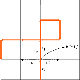
Figure 2. A NBW segment on a grid.

The network $(G,\circ,\circ^{\prime})$ can roughly be thought of as choosing the root of $G$ according to a degree bias from the distribution of $(G,\circ)$, and then choosing $\circ^{\prime}$ as a uniform random neighbour of $\circ$. If $(G,\circ)$ is a fixed finite graph with a uniform random root $\circ$ then $(G,\circ,\circ^{\prime})$ is rooted at a uniform random directed edge of $G$.

Also, for a random edge rooted network $(G,e)=(G,e^{-},e^{+})\in\mathcal{G}^{**}$, we define its reversal $(G,\overset{\shortleftarrow}{e})$ as the random edge rooted network whose law satisfies the following for all bounded measurable $f:\mathcal{G}^{**}\to\mathbb{R}$:

$$\mathbf{E}\left[f(G,\overset{\shortleftarrow}{e})\right]=\mathbb{E}_{(G,e)}\left[f(G,e^{+},e^{-})\right].$$

Lemma 2.1 (Stationarity of NBW).

Let $(G,\circ)$ be a unimodular network with no leaves almost surely and satisfying $\mathbf{E}\left[\mathrm{deg}(\circ)\right]<\infty$. Let $(G_{0},e_{0}),(G_{1},e_{1}),\ldots$ be the NBW on $(G,\circ)$. Then the reversal $(G,\overset{\shortleftarrow}{e}_{0})$ has the same law as $(G,e_{0})$, and each $(G_{n},e_{n})$ has the same law as $(G_{0},e_{0})$.

Proof.

If $f:\mathcal{G}^{**}\to[0,\infty)$ is measurable then

$$\mathbf{E}\left[f(G_{0},\overset{\shortleftarrow}{e}_{0})\right]=\frac{\,\mathbf{E}\left[\sum_{x:x\sim\circ}f(G,x,\circ)\right]}{\mathbf{E}\left[\mathrm{deg}(\circ)\right]}=\frac{\mathbf{E}\left[\,\sum_{x:x\sim\circ}f(G,\circ,x)\right]}{\mathbf{E}\left[\mathrm{deg}(\circ)\right]}=\mathbf{E}\left[f(G_{0},e_{0})\right],$$

where the second equality uses the mass transport principle (1.1). This shows that $(G_{0},\overset{\shortleftarrow}{e}_{0})$ has the same law as $(G_{0},e_{0})$.

For the second claim, it suffices to show that $(G_{1},e_{1})$ has the same law as $(G_{0},e_{0})$. For $f$ as above, we see from the definition of a NBW step that

$$\mathbf{E}\left[f(G_{1},e_{1})\right] =\mathbb{E}_{(G,\circ,\circ^{\prime})}\left[\sum_{z\sim\circ^{\prime},\,z\neq\circ}\frac{f(G,\circ^{\prime},z)}{\deg(\circ^{\prime})-1}\right]$$

(2.2) $$=\dfrac{\mathbb{E}_{(G,\circ)}\left[\sum_{x,z\in V(G)}\frac{f(G,x,z)}{\deg(x)-1}\mathbf{1}_{\{z\neq\circ,z\sim x,x\sim\circ\}}\right]}{\mathbf{E}\left[\mathrm{deg}(\circ)\right]}.$$

The function $F:\mathcal{G}^{**}\to[0,\infty)$ defined by

$$F(G,y,z)=\sum_{x\in V(G)}\frac{f(G,x,z)}{\deg(x)-1}\mathbf{1}_{\{z\neq y,x\sim z,x\sim y\}}$$

is an isomorphism invariant. The mass transport principle applied to it gives

$$\mathbf{E}\left[\sum_{z\in V(G)}F(\circ,z)\right]=\mathbf{E}\left[\sum_{z\in V(G)}F(z,\circ)\right].$$

The l.h.s. above is the numerator of (2.2). The term inside $\mathbf{E}\left[\cdot\right]$ on the r.h.s. is

$$\sum_{x,z\in V(G)}\frac{f(G,x,\circ)}{\deg(x)-1}\mathbf{1}_{\{z\neq\circ,x\sim\circ,x\sim z\}}= \sum_{x\in V(G)}\frac{f(G,x,\circ)}{\deg(x)-1}\sum_{z\in V(G)}\mathbf{1}_{\{z\neq\circ,x\sim\circ,x\sim z\}}$$

$$=\sum_{x:x\sim\circ}f(G,x,\circ).$$

Therefore, $\mathbf{E}\left[\mathrm{deg}(\circ)\right]\cdot\mathbf{E}\left[f(G_{1},e_{1})\right]=\mathbf{E}\left[\sum_{x:x\sim\circ}f(G,x,\circ)\right]=\mathbf{E}\left[\sum_{x:x\sim\circ}f(G,\circ,x)\right]$. This proves $\mathbf{E}\left[f(G_{1},e_{1})\right]=\mathbf{E}\left[f(G_{0},e_{0})\right]$. ∎

2.3. Entropy

We mention some concepts of Shannon entropy that we will use; for a reference see [7]. Let $X$ be a random variable with values in a countable state space $\Omega$. If $p(x)$ is the probability density of $X$ then the entropy of $X$ is

$$H[X]=\sum_{x\in\Omega}-p(x)\log p(x)=\mathbb{E}_{X}\left[-\log p(X)\right].$$

Let $(X,Y)$ be jointly distributed on $\Omega^{2}$ and let $p(y|x)$ be the conditional density of $Y$ given $\{X=x\}$ ($p(y|x)\equiv 0$ if $p(x)=0$). The conditional entropy of $Y$ given $X$ is

$$H[Y|X]=\mathbb{E}_{X}\left[\sum_{y\in\Omega}-p(y|X)\log p(y|X)\right].$$

If $H[X,Y]$ and $H[X]$ are both finite then $H[Y|X]=H[X,Y]-H[X]$. If $Y$ is measurable with respect to $X$ then $H[Y|X]=0$. If $(X,Y,Z)$ are jointly distributed such that $Y$ is conditionally independent of $Z$ given $X$ then $H[Y|X,Z]=H[Y|X]$. If $(X_{0},\ldots,X_{n})$ are jointly distributed then the chain rule of entropy states

$$H[X_{0},\ldots,X_{n}]=H[X_{0}]+H[X_{1}|X_{0}]+H[X_{2}|X_{1},X_{0}]+\cdots+H[X_{n}|X_{n-1},\ldots,X_{0}].$$

Entropy of the NBW step.

If $(G,x,y)\in\mathcal{G}^{**}$ is edge rooted without leaves then $H[\mathrm{NBW}(G,x,y)\mid(G,x,y)]=\log(\deg(y)-1)$. This implies that if $(G,\circ,\circ^{\prime})$ is a random edge rooted graph without leaves, almost surely, then $H[\mathrm{NBW}(G,\circ,\circ^{\prime})\mid(G,\circ,\circ^{\prime})]=\mathbb{E}_{(G,\circ,\circ^{\prime})}[\log(\deg(\circ^{\prime})-1)]$. In particular, if $(G,\circ,\circ^{\prime})$ is derived from a unimodular network $(G,\circ)$ via (2.1), then the edge reversal invariance of $(G,\circ,\circ^{\prime})$ (Lemma 2.1) applied to $\mathbb{E}_{(G,\circ,\circ^{\prime})}[\log(\deg(\circ^{\prime})-1)]$ gives the entropy of a NBW step on a unimodular network:

(2.3) $$H[\mathrm{NBW}(G,\circ,\circ^{\prime})\mid(G,\circ,\circ^{\prime})]=\mathbb{E}_{(G,\circ,\circ^{\prime})}\left[\log(\mathrm{deg}(\circ)-1)\right]=\frac{\mathbf{E}\left[\mathrm{deg}(\circ)\log(\mathrm{deg}(\circ)-1)\right]}{\mathbf{E}\left[\mathrm{deg}(\circ)\right]}.$$

3. Spectral radius of unimodular trees

In order to prove Theorem 1 we will consider unimodular networks with edge weights and bound the expectation of weighted closed walks. By choosing appropriate weights we will deduce both statements in Theorem 1. Let $(T,x)\in\mathcal{G}^{*}$ be a tree. Let $w\in W_{2k}(T,x)$ and let the sequence of vertices visited by $w$ be denoted $w_{0}=x,w_{1},\ldots,w_{2k}=x$. Let $e_{j}=(w_{j-1},w_{j})$. The height profile of $w$ is the function $h_{w}:\{0,1,\ldots,2k\}\to\{0,1,2,\ldots\}$ defined by $h_{w}(j)=\mathrm{dist}_{T}(x,w_{j})$. The height profile is a Dyck path of length $2k$. The forward steps of $w$ is the sequence of $k$ directed edges $e_{j_{1}},\ldots,e_{j_{k}}$ for which $h_{w}(j_{i})-h_{w}(j_{i}-1)=1$, and such a $j_{i}$ is a forward time. The walk $w$ is uniquely determined by its height profile and forward steps.

Let $c:\mathcal{G}^{**}\to[0,\infty)$ be a weight function such that for some $\delta>0$ if $(G,x,y)$ is rooted at an edge $(x,y)$ then $c(G,x,y)\geq\delta$. The weighted number of closed walks of length $2k$ in $(T,x)$ is defined as

$$W_{2k}(T,x,c)=\sum_{w\in W_{2k}(T,x)}\,\prod_{i=1}^{2k}\,c(T,e_{i}).$$

We will write $c(G,x,y)$ as $c(x,y)$ when there is no confusion.

Define the symmetric weight function $\kappa(x,y)=c(x,y)c(y,x)$. Note that if $w$ is a closed walk on a tree then for every forward step $e_{i}$ of $w$ there is a unique accompanying step $e_{j}$ in the reverse direction to $e_{i}$ at some time $j>i$. Indeed, $j$ is the first time $w$ traverses the reversal of $e_{i}$ after time $i$. Pairing up every forward step with its accompanying reversal we see that

$$W_{2k}(T,x,c)=\sum_{w\in W_{2k}(T,x)}\;\prod_{i\,\text{forward time of}\,w}\kappa(e_{i}).$$

Let $\mathrm{Dyck}(k)$ denote the set of all Dyck paths of length $2k$, which are the set of all possible height profiles of walks in $W_{2k}(T,x)$. For a neighbour $y$ of $x$, let $W_{2k}(T,x,y,h,c)$ be the weighted sum over all walks in $W_{2k}(T,x)$ whose first step is towards $y$ and which has height profile $h$, except without accounting for the first weighted step:

$$W_{2k}(T,x,y,h,c)=\sum_{\begin{subarray}{c}w\in W_{2k}(T,x)\\ w_{1}=y,\,h_{w}=h\end{subarray}}\;\prod_{\begin{subarray}{c}\text{forward times}\,i,\\ i>1\end{subarray}}\kappa(e_{i}).$$

Conditioning on the height profile and the first step of a walk gives

(3.1) $$W_{2k}(T,x,c)=\sum_{h\in\mathrm{Dyck}(k)}\;\sum_{y:y\sim x}\kappa(x,y)W_{2k}(T,x,y,h,c).$$

Proposition 1.

Let $(T,\circ)$ be a unimodular tree with finite expected degree and no leaves almost surely. Recall the edge rooted tree $(T,\circ,\circ^{\prime})$ derived from $(T,\circ)$ via (2.1). If $h\in\mathrm{Dyck}(k)$, then

$$\mathbf{E}\left[W_{2k}(T,\circ,\circ^{\prime},h,c)\right]\geq\Big{\{}(k-1)H\left[\mathrm{NBW}(T,\circ,\circ^{\prime})\mid(T,\circ,\circ^{\prime})\right]+2(k-1)\mathbf{E}\left[\log c(T,\circ,\circ^{\prime})\right]\Big{\}}.$$

Proof of Proposition 1

Jensen’s inequality implies

(3.2) $$\mathbf{E}\left[W_{2k}(T,\circ,\circ^{\prime},h,c)\right]\geq\exp\left\{\mathbf{E}\left[\log W_{2k}(T,\circ,\circ^{\prime},h,c)\right]\right\}.$$

Let $(T,x,y)\in\mathcal{G}^{**}$ be an edge rooted tree with no leaves. We define a probability distribution on the set $\{w\in W_{2k}(T,x):w_{1}=y,h_{w}=h\}$. Every element of this set is encoded as a sequence of edge rooted trees $(T_{1},e_{1})$, $\ldots$, $(T_{2k},e_{2k})$, where $(T_{1},e_{1})=(T,x,y)$ and $(T_{i},e_{i})$ is obtained from $(T_{i-1},e_{i-1})$ by moving along the $i$-th edge of the walk. Therefore, consider the following probability distribution $(T_{1},f_{1}),\ldots,(T_{2k},f_{2k})$ on the set.

First, $(T_{1},f_{1})=(T,x,y)$. Now consider a stack $S$ of forward times of $h$ that is initialized to $S=[1]$. For $i>1$, if $i$ is a forward time then set $(T_{i},f_{i})=\mathrm{NBW}(T_{i-1},f_{i-1})$ and append $i$ to $S$ by updating $S=[S,i]$. If $i$ is a backward time, let $\ell$ be the last element of $S$ and set $(T_{i},f_{i})=(T_{\ell},\overset{\shortleftarrow}{f}_{\ell})$, that is, the reversal of $(T_{\ell},f_{\ell})$. Then update $S$ by removing $\ell$ from the end of $S$. Figure 3 provides an illustration.

Observe that the walk is at the root whenever $S$ in empty and then the next step is a forward step. The stack $S$ is determined from $h$ and non random. Note that at a forward time $i$, $(T_{i},f_{i})$ is conditionally independent of $(T_{1},f_{1}),\ldots,(T_{i-2},f_{i-2})$ given $(T_{i-1},f_{i-1})$ due to the Markov property of the NBW. During a backward time $i$, $(T_{i},f_{i})$ is a (measurable) function of the history $(T_{1},f_{1}),\ldots,(T_{i-1},f_{i-1})$.

Figure 3. A 6-step height profile and a closed walk on the tree associated to it. Steps 3 and 4 each have two possible choices for a forward step. The stack $S$ updates as $[1]\to[\,]\to[3]\to[3,4]\to[3]\to[\,]$.

Lemma 3.1.

Let $(T,x,y)$, $h$ and $(T_{1},f_{1}),\ldots,(T_{2k},f_{2k})$ be as above. Then,

$$\log W_{2k}(T,x,y,h,c)\geq\sum_{\begin{subarray}{c}\text{forward times}\,i,\\ i>1\end{subarray}}H\left[(T_{i},f_{i})\,|\,(T_{i-1},f_{i-1})\right]+\mathbf{E}\left[\log\kappa(T_{i},f_{i})\right].$$

Proof.

For two probability distributions of a countable set $\Omega$ with densities $p$ and $q$, the Kullback-Leibler Divergence of $p$ from $q$ is $D(p||q)=\sum_{\omega\in\Omega}\log\big{(}\frac{p(\omega)}{q(\omega)}\big{)}\,p(\omega)$. The divergence is nonnegative, which gives

$$\sum-\log(q(\omega))\,p(\omega)\geq\sum-\log(p(\omega))\,p(\omega).$$

If $q$ has the form $q(\omega)=e^{E(\omega)}/Z$, then we get $\log Z\geq H[X]+\mathbf{E}\left[E(X)\right]$, where $X$ is a random variable with probability density $p$.

We apply this to $\Omega=\{w\in W_{2k}(T,x):w_{1}=y,h_{w}=h\}$, X being the process $(T_{1},f_{1}),\ldots,(T_{2k},f_{2k})$, and $E(w)=\sum_{\text{forward time}\,i>1}\log\kappa(e_{i})$ for a walk $w\in\Omega$. We deduce that

$$\log W_{2k}(T,x,y,h,c)\geq H\left[(T_{1},f_{1}),\ldots,(T_{2k},f_{2k})\right]+\sum_{\begin{subarray}{c}\text{forward times}\,i,\\ i>1\end{subarray}}\mathbf{E}\left[\log\kappa(T_{i},f_{i})\right].$$

We use the chain rule to calculate $H[(T_{1},f_{1}),\ldots,(T_{2k},f_{2k})]$. Note that $H[(T_{1},f_{1})]$ equals 0 because $(T_{1},f_{1})$ is non random. Therefore,

$$H\left[(T_{1},f_{1}),\ldots,(T_{2k},f_{2k})\right]=\sum_{i=2}^{2k}H\left[(T_{i},f_{i})\mid(T_{i-1},f_{i-1}),\ldots,(T_{1},f_{1})\right].$$

During a backward time $i$, $H[(T_{i},f_{i})\mid(T_{i-1},f_{i-1})\ldots(T_{1},f_{1})]=0$ because $(T_{i},f_{i})$ is determined from $(T_{1},f_{1}),\ldots,(T_{i-1},f_{i-1})$ and the stack $S$. At a forward time $i>1$, the conditional independence of $(T_{i},f_{i})$ from $(T_{1},f_{1}),\ldots,(T_{i-2},f_{i-2})$ given $(T_{i-1},f_{i-1})$ implies

$$H[(T_{i},f_{i})\mid(T_{i-1},f_{i-1}),\ldots,(T_{1},f_{1})]=H[(T_{i},f_{i})\mid(T_{i-1},f_{i-1})].$$

Therefore,

$$H\left[(T_{1},f_{1}),\ldots,(T_{2k},f_{2k})\right]=\sum_{\begin{subarray}{c}i\;\text{forward time}\\ i>1\end{subarray}}H[(T_{i},f_{i})\mid(T_{i-1},f_{i-1})].\qed$$

Let $(T_{1},\circ_{1},\circ^{\prime}_{1}),\ldots,(T_{2k},\circ_{2k},\circ^{\prime}_{2k})$ be the law of the process $(T_{1},f_{1}),\ldots,(T_{2k},f_{2k})$ started from the random edge rooted graph $(T,\circ,\circ^{\prime})$. Applying Lemma 3.1 to $(T,\circ,\circ^{\prime})$ and taking expectation over $(T,\circ,\circ^{\prime})$ gives

$$\mathbf{E}\left[\log W_{2k}(T,\circ,\circ^{\prime},h,c)\right]\geq\sum_{\begin{subarray}{c}\text{forward times}\,i,\\ i>1\end{subarray}}H[(T_{i},\circ_{i},\circ^{\prime}_{i})|(T_{i-1},\circ_{i-1},\circ^{\prime}_{i-1})]+\mathbf{E}\left[\log\kappa(T_{i},\circ_{i},\circ^{\prime}_{i})\right].$$

We claim that every $(T_{i},\circ_{i},\circ^{\prime}_{i})$ has the law of $(T,\circ,\circ^{\prime})$. This is certainly the case for $i=1$. Assume that this is the case for each of the graphs $(T_{1},\circ_{1},\circ^{\prime}_{1}),\ldots,(T_{i-1},\circ_{i-1},\circ^{\prime}_{i-1})$. Then $(T_{i},\circ_{i},\circ^{\prime}_{i})$ either has the law of the tree $\mathrm{NBW}(T_{i-1},\circ_{i-1},\circ^{\prime}_{i-1})$, or the reversal of one of $(T_{1},\circ_{1},\circ^{\prime}_{1}),\ldots,(T_{i-1},\circ_{i-1},\circ^{\prime}_{i-1})$. By Lemma 2.1, both these operations preserve the law of $(T,\circ,\circ^{\prime})$. So the claim follows by induction.

Consequently, for every $i$,

(3.3) $$H[(T_{i},\circ_{i},\circ^{\prime}_{i})\mid(T_{i-1},\circ_{i-1},\circ^{\prime}_{i-1})] =H[\mathrm{NBW}((T,\circ,\circ^{\prime}))\mid(T,\circ,\circ^{\prime})],$$

$$\mathbf{E}\left[\log\kappa(T_{i},\circ_{i},\circ^{\prime}_{i})\right] =\mathbf{E}\left[\log\kappa(T,\circ,\circ^{\prime})\right].$$

As there are $k-1$ forward times $i>1$, we combine (3.3) with (3.2) to conclude that

$$\mathbf{E}\left[W_{2k}(T,\circ,\circ^{\prime},h,c)\right]\geq\exp\big{\{}(k-1)H[\mathrm{NBW}(T,\circ,\circ^{\prime})\mid(T,\circ,\circ^{\prime})]+(k-1)\mathbf{E}\left[\log\kappa(T,\circ,\circ^{\prime})\right]\big{\}}.$$

The edge reversal invariance of $(T,\circ,\circ^{\prime})$ implies $\mathbf{E}\left[\log\kappa(T,\circ,\circ^{\prime})\right]=2\mathbf{E}\left[\log c(T,\circ,\circ^{\prime})\right]$. This completes the proof of Proposition 1.

Theorem 1 is proved using Proposition 1 as follows. Since $\kappa(G,x,y)\geq\delta^{2}$ for every edge rooted graph $(G,x,y)$, (3.1) implies

$$\mathbf{E}\left[W_{2k}(T,\circ,c)\right]\geq\delta^{2}\,|\mathrm{Dyck}(k)|\,\mathbf{E}\left[\mathrm{deg}(\circ)\right]\mathbf{E}\left[W_{2k}(T,\circ,\circ^{\prime}c)\right].$$

The number of Dyck paths of length $2k$ is the Catalan number $\frac{1}{k+1}\binom{2k}{k}$. It is easily seen that $|\mathrm{Dyck}(k)|^{1/2k}\to 2$ as $k\to\infty$. Proposition 1 thus implies

(3.4) $$\liminf_{k\to\infty}\,\mathbf{E}\left[|W_{2k}(T,\circ,c)\right]^{1/2k}\geq 2\exp\left\{\frac{1}{2}H[\mathrm{NBW}(T,\circ,\circ^{\prime})|(T,\circ,\circ^{\prime})]+\mathbf{E}\left[\log c(T,\circ,\circ^{\prime})\right]\right\}.$$

Plugging the expression for $H[\mathrm{NBW}(T,\circ,\circ^{\prime})\mid(T,\circ,\circ^{\prime})]$ from (2.3), and setting $c(G,x,y)\equiv 1$ in (3.4), provides the first lower bound to $\rho(T)$ stated in Theorem 1. If $(T,\circ)$ has degrees bounded by $\Delta$ almost surely, then the first lower bound to $\rho_{\mathrm{SRW}}(T)$ stated in Theorem 1 follows from (3.4) by having $c(G,x,y)=1/\mathrm{deg}_{G}(x)$ and $\delta=1/\Delta$.

The second group of lower bounds in Theorem 1 are derived from convexity. Jensen’s inequality applied to $x\to x\log(x-1)$ for $x\geq 2$ gives

$$\mathbf{E}\left[\mathrm{deg}(\circ)\log(\mathrm{deg}(\circ)-1)\right]\geq\mathbf{E}\left[\mathrm{deg}(\circ)\right]\log(\mathbf{E}\left[\mathrm{deg}(\circ)\right]-1),$$

which provides the second lower bound to $\rho(T)$. Jensen’s inequality applied to $x\to e^{x}$ for the probability measure $f\to\mathbf{E}\left[\mathrm{deg}(\circ)f\right]/\mathbf{E}\left[\mathrm{deg}(\circ)\right]$ gives

$$\exp\left\{\frac{\mathbf{E}\left[\mathrm{deg}(\circ)\log\mathrm{deg}(\circ)\right]}{\mathbf{E}\left[\mathrm{deg}(\circ)\right]}\right\}\leq\frac{\mathbf{E}\left[\mathrm{deg}(\circ)^{2}\right]}{\mathbf{E}\left[\mathrm{deg}(\circ)\right]}.$$

Taking reciprocals above in combination with the bound

$$\mathbf{E}\left[\mathrm{deg}(\circ)\log(\mathrm{deg}(\circ)-1)\right]\geq\mathbf{E}\left[\mathrm{deg}(\circ)\right]\log(\mathbf{E}\left[\mathrm{deg}(\circ)\right]-1)$$

provides the second stated lower bound to $\rho_{\mathrm{SRW}}(T)$. ∎

4. Alon-Boppana bound and volume growth: proofs of Theorems 2, 3 and 4

4.1. Proof of Part I of Theorem 2

Since $\mu_{G_{n}}\to\mu_{G}$ weakly, we have $\liminf_{n}\mu_{G_{n}}(|x|>a)\geq\mu_{G}(|x|>a)$ for every $a$. Therefore, since $\rho(G)<\infty$, Lemma 4.1 below implies that

(4.1) $$\liminf_{n}\,\mu_{G_{n}}\left(\{|x|>\rho(T_{G})-\epsilon\}\right)\geq\frac{\mathbf{E}\left[|W_{2k}(T_{G},\circ)|\right]-(\rho(T_{G})-\epsilon)^{2k}}{\rho(G)^{2k}}\;\;\text{for every}\;\;k.$$

Since $\mathbf{E}\left[|W_{2k}(T_{G},\circ)|\right]^{1/2k}\to\rho(T_{G})$ as $k\to\infty$, we may choose a large $K$ such that $\mathbf{E}\left[|W_{2K}(T_{G},\circ)|\right]\geq(\rho(T_{G})-\frac{\epsilon}{2})^{2K}$. Then, by defining

$$c(\epsilon,\rho(G),\rho(T_{G}))=\frac{(\rho(T_{G})-\frac{\epsilon}{2})^{2K}-(\rho(T_{G})-\epsilon)^{2K}}{\rho(G)^{2K}},$$

the inequality (4.1) applied to $k:=K$ implies that $\liminf_{n}\,\mu_{G_{n}}(\{|x|>\rho(T_{G})-\epsilon\})\geq c(\epsilon,\rho(G),\rho(T_{G}))$. This completes the proof of part I of Theorem 2. ∎

Lemma 4.1.

Let $(H,\circ)$ be a unimodular network with $\rho(H)<\infty$. For $0<a<\rho(T_{H})$ and any $k\geq 0$ we have

$$\mu_{H}\left(\{|x|>a\}\right)\geq\frac{\mathbf{E}\left[|W_{2k}(T_{H},\circ)|\right]-a^{2k}}{\rho(H)^{2k}}.$$

Proof.

Let $\nu=\mu_{H}(\{|x|>a\})$. The moments of the spectral measure of $(H,\circ)$ satisfy

$$\int x^{2k}\,d\mu_{H}=\mathbf{E}\left[|W_{2k}(H,\circ)|\right]\geq\mathbf{E}\left[|W_{2k}(T_{H},\circ)|\right].$$

On the other hand, we may bound the moments from above as follows. Note that $\mu_{H}(\{|x|>\rho(H)\})=0$ by definition of the spectral radius. Therefore,

$$\int x^{2k}\,d\mu_{H} =\int_{|x|\leq a}x^{2k}\,d\mu_{H}+\int_{|x|>a}x^{2k}\,d\mu_{H}$$

$$\leq a^{2k}\,\mu_{H}(\{|x|\leq a\})+\rho(H)^{2k}\,\mu_{H}(\{|x|>a\})$$

$$=a^{2k}+\nu\left(\rho(H)^{2k}-a^{2k}\right).$$

Combining the lower and upper bounds on the moments we get that for every $k$,

$$\nu\geq\frac{\mathbf{E}\left[|W_{2k}(T_{H},\circ)|\right]-a^{2k}}{\rho(H)^{2k}-a^{2k}}\geq\frac{\mathbf{E}\left[|W_{2k}(T_{H},\circ)|\right]-a^{2k}}{\rho(H)^{2k}}.\qed$$

4.2. Proof of Part II of Theorem 2

Lemma 4.2.

Let $G$ be a finite and connected graph with 2-core $G^{\mathrm{core}}$; recall it is obtained by iteratively removing leaves from $G$ until a subgraph with no leaves remains. If $G$ is not a tree then $d_{\mathrm{av}}(G^{\mathrm{core}})\geq d_{\mathrm{av}}(G)$. Moreover, $\sigma_{j}(G)\geq\sigma_{j}(G^{\mathrm{core}})$, where $\sigma_{j}(H)=0$ by convention if $j>|H|$. (Recall $\sigma_{j}(H)$ is the $j$-th largest eigenvalue of $H$ in absolute value counted with multiplicity).

Proof.

Since $G$ is not a tree, $|E(G)|\geq|G|$. If $G^{\prime}$ is obtained from $G$ by removing a leaf then $d_{\mathrm{av}}(G^{\prime})=2(|E(G)|-1)/(|G|-1)\geq d_{\mathrm{av}}(G)$ since $|E(G)|\geq|G|$. Moreover, the adjacency matrix of $G^{\prime}$ is a principal minor of the adjacency matrix of $G$. Suppose $\lambda_{1}\geq\lambda_{2}\geq\cdots\geq\lambda_{n}$ are the $n=|G|$ eigenvalues of $G$, and $\nu_{1}\geq\nu_{2}\geq\cdots\geq\nu_{n-1}$ are the eigenvalues of $G^{\prime}$. From the Cauchy interlacing theorem we have $\lambda_{1}\geq\nu_{1}\geq\lambda_{2}\geq\nu_{2}\geq\cdots\geq\nu_{n-1}\geq\lambda_{n}$. This implies that $\sigma_{j}(G)\geq\sigma_{j}(G^{\prime})$ for every $j$.

The observations above imply $d_{\mathrm{av}}(G^{\mathrm{core}})\geq d_{\mathrm{av}}(G)$ and $\sigma_{j}(G)\geq\sigma_{j}(G^{\mathrm{core}})$. ∎

We now prove part II of the theorem. Let $G_{n_{i}}$ be a subsequence such that $\liminf_{n}\,\sigma_{j}(G_{n})=\lim_{i}\,\sigma_{j}(G_{n_{i}})$. Clearly, $\liminf_{i}\,2\sqrt{d_{\mathrm{av}}(G_{n_{i}})-1}\geq\liminf_{n}\,2\sqrt{d_{\mathrm{av}}(G_{n})-1}$. Therefore, it is enough to show that $\liminf_{i}\,\sigma_{j}(G_{n_{i}})\geq\liminf_{i}\,2\sqrt{d_{\mathrm{av}}(G_{n_{i}})-1}$. Henceforth, we denote the subsequence $G_{n_{i}}$ as $G_{n}$ and $\sigma_{j}=\lim_{i}\,\sigma_{j}(G_{n_{i}})$. In the new notation, we must show that

(4.2) $$\sigma_{j}\geq\liminf_{n}\,2\sqrt{d_{\mathrm{av}}(G_{n})-1}\,.$$

First, suppose it is the case that for an infinite subsequence $G_{n_{k}}$ of $G_{n}$ we have that $|G^{\mathrm{core}}_{n_{k}}|\to\infty$. It suffices to show that $\sigma_{j}\geq\liminf_{k}\,2\sqrt{d_{\mathrm{av}}(G_{n_{k}})-1}$ because the latter limit infimum is an upper bound to $\liminf_{n}\,2\sqrt{d_{\mathrm{av}}(G_{n})-1}$. Let us denote the subsequence $G_{n_{k}}$ as $H_{n}$. Thus, we must show that

(4.3) $$\sigma_{j}\geq\liminf_{n}\,2\sqrt{d_{\mathrm{av}}(H_{n})-1}\,.$$

The graphs $H^{\mathrm{core}}_{n}$ are connected, have no leaves and have maximum degree at most $\Delta$. If $\circ_{n}$ is a uniform random root of $H^{\mathrm{core}}_{n}$ then the unimodular networks $(H^{\mathrm{core}}_{n},\circ_{n})$ have a subsequential limit $(G,\circ)$. Indeed, the subset of $\mathcal{G}^{*}$ consisting of rooted isomorphism classes of graphs of maximal degree $\Delta$ is compact because there are at most $\Delta^{r}$ possibilities for the $r$-neighbourhood of the root of such graphs. Prokhorov’s theorem states that Borel probability measures on a compact metric space is compact in the weak topology. This provides a subsequential limit of $(H^{\mathrm{core}}_{n},\circ_{n})$ in the local topology.

Let us reduce to a convergent subsequence $(H^{\mathrm{core}}_{n_{i}},\circ_{n_{i}})$, converging to $(G,\circ)$. Let $(T,\circ)$ be the universal cover of $(G,\circ)$. Then $(T,\circ)$ has no leaves and has maximum degree at most $\Delta$ almost surely because $(G,\circ)$ inherits these properties from the sequence $H^{\mathrm{core}}_{n_{i}}$. Part I of the theorem implies for every $\epsilon>0$,

$$\liminf_{i}\,\mu_{H^{\mathrm{core}}_{n_{i}}}(\{|x|>\rho(T)-\epsilon\})>0.$$

Since $|H^{\mathrm{core}}_{n_{i}}|\to\infty$ by assumption, $\sigma_{j}(H^{\mathrm{core}}_{n_{i}})\geq\rho(T)-\epsilon$ for all large $i$ due to the bound above. From Theorem 1 we have $\rho(T)\geq 2\sqrt{\mathbf{E}\left[\deg(\circ)\right]-1}=\lim_{i}\,2\sqrt{d_{\mathrm{av}}(H^{\mathrm{core}}_{n_{i}})-1}$. Therefore, since $\epsilon$ is arbitrary,

(4.4) $$\liminf_{i}\,\sigma_{j}(H^{\mathrm{core}}_{n_{i}})\geq\liminf_{i}\,2\sqrt{d_{\mathrm{av}}(H^{\mathrm{core}}_{n_{i}})-1}\,.$$

Lemma 4.2 implies $\sigma_{j}(H_{n_{i}})\geq\sigma_{j}(H^{\mathrm{core}}_{n_{i}})$. Taking limit infimum in $i$ implies

(4.5) $$\sigma_{j}\geq\liminf_{i}\sigma_{j}(H^{\mathrm{core}}_{n_{i}}).$$

Indeed, $\sigma_{j}$ is the limit of $\sigma_{j}(H_{n_{i}})$ because $H_{n_{i}}$ is a subsequence of $G_{n}$ and $\sigma_{j}(G_{n})$ converges to $\sigma_{j}$ by assumption. Lemma 4.2 also implies that

(4.6) $$2\,\sqrt{d_{\mathrm{av}}(H^{\mathrm{core}}_{n_{i}})-1}\geq 2\,\sqrt{d_{\mathrm{av}}(H_{n_{i}})-1}\,.$$

The required inequality in (4.3) follows by combining the inequality in (4.5) with the one from (4.4), followed by the inequality in (4.6).

We are left to consider the case where the core graphs of the sequence $G_{n}$ have bounded size, possibly being empty. Due to compactness, as explained above, the unimodular networks $(G_{n},\circ_{n})$, where $\circ_{n}$ is a uniform random root of $G_{n}$, have a subsequential limit $(G,\circ)$. We claim that $(G,\circ)$ is an infinite unimodular tree of expected degree $2$.

Indeed, $(G,\circ)$ is infinite almost surely because $G_{n}$ is connected and $|G_{n}|\to\infty$. To see that $(G,\circ)$ is a tree observe that the graph induced on $G_{n}\setminus G^{\mathrm{core}}_{n}$ contains no cycles. Thus $B_{r}(G_{n},\circ_{n})$ is a tree so long as $\circ_{n}$ is not within distance $r$ of $G^{\mathrm{core}}_{n}$, and this happens with probability at least $1-\frac{|G^{\mathrm{core}}_{n}|\Delta^{r}}{|G_{n}|}\to 1$. This implies that the finite neighbourhood sampling statistics of $(G,\circ)$ are supported on trees, and thus, $(G,\circ)$ is a tree.

Now we argue that $(G,\circ)$ has expected degree 2. Suppose $l_{n}$ is the number of vertices removed from $G_{n}$ during the leaf peeling procedure that generates $G^{\mathrm{core}}_{n}$. Then $l_{n}\to\infty$ as $n\to\infty$ because $|G^{\mathrm{core}}_{n}|$ remains bounded. Moreover,

$$|G_{n}|=|G^{\mathrm{core}}_{n}|+l_{n}\;\;\text{and}\;\;|E(G_{n})|=|E(G^{\mathrm{core}}_{n})|+l_{n}.$$

Therefore,

$$d_{\mathrm{av}}(G_{n})=2\,\frac{|E(G^{\mathrm{core}}_{n})|+l_{n}}{|G^{\mathrm{core}}_{n}|+l_{n}}\,\longrightarrow\,2,$$

which shows that $(G,\circ)$ has expected degree 2 because $d_{\mathrm{av}}(G_{n})$ converges to it due to the graphs $G_{n}$ having uniformly bounded degrees.

Now we claim that $\rho(G)\geq 2$. As $(G,\circ)$ is infinite, there is an infinite one ended path starting from $\circ$. Therefore, $|W_{2k}(G,\circ)|$ is at least the number of closed walks of length $2k$ on an infinite one ended path starting from its initial leaf vertex. This quantity is the Catalan number $C_{k}=\frac{1}{k+1}\binom{2k}{k}$. Thus, $\mathbf{E}\left[|W_{2k}(G,\circ)|\right]\geq C_{k}$ and we conclude that $\rho(G)\geq 2$ because $C_{k}^{1/2k}\to 2$.

The tree $(G,\circ)$ is its own universal cover. Using part I of the theorem and arguing as before we deduce that $\sigma_{j}=\lim_{n}\,\sigma_{j}(G_{n})\geq 2$. On the other hand,

$$\liminf_{n}\,2\sqrt{d_{\mathrm{av}}(G_{n})-1}\leq 2\sqrt{\mathbb{E}_{(G,\circ)}[\deg(\circ)]-1}=2.$$

These bounds imply the required inequality in (4.2) and completes the proof of part II of the theorem. ∎

4.3. Proof of Theorem 3

For a finite graph $G$ let us denote

$$\bar{D}(G)=\frac{2\sqrt{d_{\mathrm{av}}(G)-1}}{\frac{1}{2|E(G)|}\sum_{x\in G}(\deg{x})^{2}}.$$

Note that $\bar{D}(G)$ is a continuous function in the topology of local convergence since $2|E(G)|=d_{\mathrm{av}}(G)|G|$.

First we shall consider the proof when the sequence of graph $G_{n}$ has no leaves. Then given $\epsilon>0$, consider a subsequence $G_{n_{i}}$ such that $\mu^{\mathrm{SRW}}_{G_{n_{i}}}(\{|x|>\bar{D}(G_{n_{i}})-\epsilon\})$ converges to the limit infimum of $\mu^{\mathrm{SRW}}_{G_{n}}(\{|x|>\bar{D}(G_{n})-\epsilon\})$. Due to compactness, there is a further locally convergent subsequence $(G_{n_{i_{j}}},\circ_{n_{i_{j}}})\to(G,\circ)$. It suffices to prove the claim for this convergent subsequence. Denote the sequence of graphs $G_{n_{i_{j}}}$ as $H_{n}$.

Arguing as in the proof of part I of Theorem 2 we see that

$$\liminf_{n\to\infty}\,\mu^{\mathrm{SRW}}_{H_{n}}\left(\left\{|x|>\rho_{\mathrm{SRW}}(T_{G})-\frac{\epsilon}{2}\right\}\right)>0,$$

where $(G,\circ)$ is the limit. Theorem 1 applied to its universal cover $T_{G}$ implies

$$\rho_{\mathrm{SRW}}(T_{G})\geq\bar{D}(G,\circ)=:\frac{2\,\mathbf{E}\left[\mathrm{deg}(\circ)\right]\sqrt{\mathbf{E}\left[\mathrm{deg}(\circ)\right]-1}}{\mathbf{E}\left[\mathrm{deg}(\circ)^{2}\right]}.$$

Observe that $\bar{D}(H_{n})\to\bar{D}(G,\circ)$ because $(H_{n},\circ_{n})$ converges to $(G,\circ)$ and all the graphs are of bounded degree. Thus, for all sufficiently large $n$, we have $\bar{D}(G,\circ)\geq\bar{D}(H_{n})-\frac{\epsilon}{2}$. For any such $n$,

$$\mu^{\mathrm{SRW}}_{H_{n}}(\{|x|>\bar{D}(H_{n})-\epsilon\})\geq\mu^{\mathrm{SRW}}_{H_{n}}(\{|x|>\rho_{\mathrm{SRW}}(T_{G})-\frac{\epsilon}{2}\}).$$

This implies the required claim for the sequence $H_{n}$ and completes the proof of the theorem when the sequence $G_{n}$ has no leaves.

For the general case of $|G^{\mathrm{core}}_{n}|/|G_{n}|\to 1$, we will use the following two lemmas.

Lemma 4.3.

Let $G$ be a finite and connected graph with a non-empty 2-core. Then

$$\mu_{G}^{\mathrm{SRW}}(|x|>a)\geq\mu_{G^{\mathrm{core}}}^{\mathrm{SRW}}(|x|>a)-10\log\big{(}|G|/|G^{\mathrm{core}}|\big{)}.$$

Proof.

Suppose that $G$ has $n$ vertices and $|G^{\mathrm{core}}|=|G|-m$. Let $P$ be the Markov operator of $G$, $D$ the diagonal matrix of vertex degrees, and $A$ the adjacency matrix. Write $d_{x}=\mathrm{deg}(x)$ for a vertex $x$ of $G$.

Observe that $P=D^{-1}A$, so $P=D^{-1/2}(D^{-1/2}AD^{-1/2})D^{1/2}$. Hence $P$ has the same eigenvalues as the symmetric matrix $L=D^{-1/2}AD^{-1/2}$. If $\mu_{L}$ is the empirical measure for the eigenvalues of $L$, then $\mu^{\mathrm{SRW}}_{G}(|x|>a)=\mu_{L}(|x|>a)$.

Let $u$ be a leaf of $G$ with neighbour $v$ and consider the reduced graph $G^{\prime}=G\setminus\{u\}$. Let $\hat{L}$ be the submatrix of $L$ obtained by removing the row and column associated to vertex $u$. By the Cauchy interlacing theorem,

(4.7) $$\mu_{L}(|x|>a)\geq\mu_{\hat{L}}(|x|>a)(1-\frac{1}{n})\geq\mu_{\hat{L}}(|x|>a)-\frac{1}{n}.$$

If $L^{\prime}$ is the $L$-matrix associated to $G^{\prime}$ then

$$L^{\prime}(x,y)=\frac{\mathbf{1}_{\{x\sim y\,\text{in}\,G\}}}{\sqrt{(d_{x}-\mathbf{1}_{\{x=v\}})(d_{y}-\mathbf{1}_{\{y=v\}})}}\quad(x,y\neq u).$$

Note $L(x,y)=\mathbf{1}_{\{x\sim y\,\text{in}\,G\}}/\sqrt{d_{x}d_{y}}$. Consequently, $L^{\prime}=\hat{L}+E$ where

$$E(x,y)=\frac{d_{y}^{-1/2}\mathbf{1}_{\{x=v,\,y\sim b\}}+d_{x}^{-1/2}\mathbf{1}_{\{y=v,\,x\sim v\}}}{\sqrt{d_{v}-1}(\sqrt{d_{v}}+\sqrt{d_{v}-1})}\quad(x,y\neq u).$$

The matrix $E$ is symmetric with rank at most 2. Indeed, only the row and column associated to vertex $v$ is non-zero. So by the Weyl interlacing theorem (see [5]),

(4.8) $$\big{|}\mu_{L^{\prime}}(|x|>a)-\mu_{\hat{L}}(|x|>a)\big{|}\leq\frac{2}{n-1}.$$

If we combine (4.7) with (4.8) we infer that

$$\mu_{G}^{\mathrm{SRW}}(|x|>a)\geq\mu_{G^{\prime}}^{\mathrm{SRW}}(|x|>a)-\frac{3}{n-1}.$$

It follows from iteration that

$$\mu_{G}^{\mathrm{SRW}}(|x|>a) \geq\mu_{G^{\mathrm{core}}}^{\mathrm{SRW}}(|x|>a)-3\Big{(}\frac{1}{n-1}+\cdots+\frac{1}{n-m}\Big{)}$$

$$\geq\mu_{G^{\mathrm{core}}}^{\mathrm{SRW}}(|x|>a)-10\log(|G|/|G^{\mathrm{core}}|).\qed$$

Lemma 4.4.

Let $G$ be a finite and connected graph with vertex degrees at most $\Delta$. Let $\frac{p}{q}$ be a rational number that is not an eigenvalue of the Markov operator of $G$ and suppose that $gcd(p,q)=1$. There is a constant depending on $q$ and $\Delta$ such that for $0<\delta<1$,

$$\mu_{G}^{\mathrm{SRW}}\Big{(}\big{[}\frac{p}{q}-\delta,\frac{p}{q}+\delta\big{]}\Big{)}\leq\frac{\mathrm{const}(q,\Delta)}{|\log\delta|}.$$

Proof.

Set $\mu=\mu_{G}^{\mathrm{SRW}}([(p/q)-\delta,(p/q)+\delta])$, let $P$ denote the Markov operator of $G$, and suppose $G$ has $n$ vertices. We may assume $|\frac{p}{q}|\leq 2$ for otherwise $\mu$ is zero.

Consider the determinant of $(p/q)I-P$ in two different ways. On the one hand, $P$ has a full set of eigenvalues inside $[-1,1]$, which implies that

(4.9) $$\big{|}\mathrm{det}\Big{(}\frac{p}{q}I-P\Big{)}\big{|}=\prod_{\text{eig.~{}val.~{}}\,\lambda}\,\big{|}\frac{p}{q}-\lambda\big{|}\leq\delta^{n\mu}\,3^{n(1-\mu)}.$$

On the other hand, consider $\ell=lcm(\mathrm{deg}(x);x\in G)$ which is at most $lcm(1,2,\ldots,\Delta)$. Now $\mathrm{det}\big{(}(p/q)I-P\big{)}=(q\ell)^{-n}\mathrm{det}(p\ell I-q\ell P)$, and the matrix $p\ell I-q\ell P$ has integer entries as well as a non-zero determinant. So $|\mathrm{det}(p\ell I-q\ell P)|\geq 1$. This implies that

(4.10) $$\big{|}\mathrm{det}\Big{(}\frac{p}{q}I-P\Big{)}\big{|}\geq(q\ell)^{-n}.$$

Comparing (4.9) with (4.10) provides the inequality from the lemma. ∎

To conclude the proof suppose $G_{n}$ is a sequence of graphs as in the theorem and $\epsilon>0$. It suffices to consider only rational values of $\epsilon$ with $0<\epsilon<1$. Due to having bounded degrees and $|G^{\mathrm{core}}_{n}|/|G_{n}|\to 1$, it is easy to see that $|\bar{D}(G_{n})-\bar{D}(G^{\mathrm{core}}_{n})|\to 0$. Now if $\bar{D}(G_{n})\leq\bar{D}(G^{\mathrm{core}}_{n})$, then $\mu_{G_{n}}^{\mathrm{SRW}}(|x|>\bar{D}(G_{n})-\epsilon)\geq\mu_{G_{n}}^{\mathrm{SRW}}(|x|>\bar{D}(G^{\mathrm{core}}_{n})-\epsilon)$.

If not, consider a rational number $r$ such that $r$ is not an eigenvalue of the Markov operator of $G_{n}$, $r\leq\bar{D}(G^{\mathrm{core}}_{n})-\epsilon$, and $|r-\bar{D}(G_{n})+\epsilon|\leq 2|\bar{D}(G^{\mathrm{core}}_{n})-\bar{D}(G_{n})|$. Since the graphs have degrees bounded by $\Delta$ it is easy to see that the denominator of $r$ remains bounded in terms of on $\epsilon$ and $\Delta$. Then by Lemma 4.4 with $\delta=2|\bar{D}(G^{\mathrm{core}}_{n})-\bar{D}(G_{n})|$, since $r\leq\bar{D}(G^{\mathrm{core}}_{n})-\epsilon\leq\bar{D}(G_{n})-\epsilon\leq r+\delta$, we find that

(4.11) $$\mu_{G_{n}}^{\mathrm{SRW}}(|x|>\bar{D}(G_{n})-\epsilon)\geq\mu_{G_{n}}^{\mathrm{SRW}}(|x|>\bar{D}(G^{\mathrm{core}}_{n})-\epsilon)-\frac{\mathrm{const}(\epsilon,\Delta)}{|\log(|\bar{D}(G^{\mathrm{core}}_{n})-\bar{D}(G_{n})|)|}.$$

The inequality (4.11) thus holds irrespective of the ordering between $\bar{D}(G_{n})$ and $\bar{D}(G^{\mathrm{core}}_{n})$. By Lemma 4.3, we may replace $\mu_{G_{n}}^{\mathrm{SRW}}$ by $\mu_{G^{\mathrm{core}}_{n}}^{\mathrm{SRW}}$ on the right hand side of (4.11) while incurring a penalty of vanishing order $\log(|G_{n}|/|G^{\mathrm{core}}_{n})$. Then considering the limit infimum and applying the previous case to $G^{\mathrm{core}}_{n}$ leads to the theorem. ∎

It may be interesting to see to what extent Theorrem 3 holds when $G^{\mathrm{core}}_{n}$ only occupies a positive fraction of $G_{n}$.

4.4. Proof of Theorem 4

Let $(T,\circ)$ be a unimodular tree with $\mathbf{E}\left[\mathrm{deg}(\circ)\right]<\infty$ and having no leaves almost surely. Let $S_{r}(T,x)=\{v\in V(T):\mathrm{dist}_{T}(x,v)=r\}$. Recall the height profile of a walk and the notation $W_{2k}(G,x,y,h,c)$ from Section 3 (around (3.1)). The vertices in $S_{r}(T,x)$ are in bijection with walks in $W_{2r}(T,x)$ whose height profile is the Dyck path consisting of $r$ forward steps followed by $r$ backward steps. Let $h$ denote this particular height profile. Then, with $c(x,y)\equiv 1$,

$$|S_{r}(T,x)|=\sum_{y\sim x}|W_{2r}(T,x,y,h,c)|.$$

Theorem 4 now follows from Proposition 1. ∎

5. Future directions

It is shown in [1] that if an infinite $d$-regular unimodular network has spectral radius $2\sqrt{d-1}$ then it must be the $d$-regular tree. It is also proved that if a sequence of finite, connected, $d$-regular graphs $G_{n}$ converges to the $d$-regular tree locally then apart from $o(|G_{n}|)$ short cycles the smallest cycle in $G_{n}$ has length of order at least $\log\log|G_{n}|$. Little is known about such results for arbitrary unimodular networks. Suppose a sequence of finite and connected graphs $G_{n}$ of growing size share a common universal cover $T$. If the spectral measures of the $G_{n}$ concentrate on $[-\rho(T),\rho(T)]$ as $n\to\infty$ then does $G_{n}$ converge to $T$ locally?

References

- [1] M. Abért, Y. Glasner, and B. Virág. The measurable Kesten theorem. Annals of Probability, 44(3):1601–1646, 2016.
- [2] D. Aldous and R. Lyons. Processes on unimodular networks. Electronic Journal of Probability, 12(54):1454–1508, 2007.
- [3] O. Angel, J. Friedman, and S. Hoory. The non-backtracking spectrum of the universal cover of a graph. Transactions of the American Mathematical Society, 367:4287–4318, 2015.
- [4] I. Benjamini and O. Schramm. Recurrence of distributional limits of finite planar graphs. Electronic Journal of Probability, 6(23), 2001.
- [5] C. Bordenave. Spectrum of random graphs. Available at http://www.math.univ-toulouse.fr/~bordenave/coursSRG.pdf, 2016.
- [6] S. M. Cioabă. Eigenvalues of graphs and a simple proof of a theorem of Greenberg. Linear Algebra and its Applications, 416:776–782, 2006.
- [7] T. M. Cover and J. A. Thomas. Elements of Information Theory. John Wiley & Sons, Inc., 2006.
- [8] G. Elek. Weak convergence of finite graphs, integrated density of states and a Cheeger type inequality. Journal of Combinatorial Theory, Series B, 98(1):62–68, 2008.
- [9] Y. Greenberg. On the Spectrum of Graphs and Their Universal Covering. PhD thesis, Hebrew University of Jerusalem, 1995.
- [10] S. Hoory. A lower bound on the spectral radius of the universal cover of a graph. Journal of Combinatorial Theory, Series B, 93:33–43, 2005.
- [11] F. Leighton. Finite common coverings of graphs. Journal of Combinatorial Theory, Series B, 33:231–238, 1982.
- [12] A. Lubotzky. Cayley graphs: eigenvalues, expanders and random walks. In Survey in Combinatorics, pages 155 – 189. Cambridge University Press, 1995.
- [13] B. Mohar. A strengthening and a multipartite generalization of the Alon-Boppana-Serre Theorem. Proceedings of the American Mathematical Society, 138:3899–3909, 2010.
- [14] A. Nilli. On the second eigenvalue of a graph. Discrete Mathematics, 91:207–210, 1991.
- [15] J.-P. Serre. Répartition asymptotique des valeurs propres de l’opérateur de Hecke . Journal of the Americal Mathematical Society, 10(1):75–102, 1997.