Breaking the Bandwidth Barrier:
Geometrical Adaptive Entropy Estimation

Abstract

Estimators of information theoretic measures such as entropy and mutual information are a basic workhorse for many downstream applications in modern data science. State of the art approaches have been either geometric (nearest neighbor (NN) based) or kernel based (with a globally chosen bandwidth). In this paper, we combine both these approaches to design new estimators of entropy and mutual information that outperform state of the art methods. Our estimator uses local bandwidth choices of $k$-NN distances with a finite $k$, independent of the sample size. Such a local and data dependent choice improves performance in practice, but the bandwidth is vanishing at a fast rate, leading to a non-vanishing bias. We show that the asymptotic bias of the proposed estimator is universal; it is independent of the underlying distribution. Hence, it can be precomputed and subtracted from the estimate. As a byproduct, we obtain a unified way of obtaining both kernel and NN estimators. The corresponding theoretical contribution relating the asymptotic geometry of nearest neighbors to order statistics is of independent mathematical interest.

1 Introduction

Unsupervised representation learning is one of the major themes of modern data science; a common theme among the various approaches is to extract maximally “informative" features via information-theoretic metrics (entropy, mutual information and their variations) – the primary reason for the popularity of information theoretic measures is that they are invariant to one-to-one transformations and that they obey natural axioms such as data processing. Such an approach is evident in many applications, as varied as computational biology [17], sociology [30] and information retrieval [23], with the citations representing a mere smattering of recent works. Within mainstream machine learning, a systematic effort at unsupervised clustering and hierarchical information extraction is conducted in recent works of [37, 35]. The basic workhorse in all these methods is the computation of mutual information (pairwise and multivariate) from i.i.d. samples. Indeed, sample-efficient estimation of mutual information emerges as the central scientific question of interest in a variety of applications, and is also of fundamental interest to statistics, machine learning and information theory communities.

While these estimation questions have been studied in the past three decades (and summarized in [40]), the renewed importance of estimating information theoretic measures in a sample-efficient manner is persuasively argued in a recent work [6], where the authors note that existing estimators perform poorly in several key scenarios of central interest (especially when the high dimensional random variables are strongly related to each other). The most common estimators (featured in scientific software packages) are nonparametric and involve $k$ nearest neighbor (NN) distances between the samples. The widely used estimator of mutual information is the one by Kraskov and Stögbauer and Grassberger [16] and christened the KSG estimator (nomenclature based on the authors, cf. [6]) – while this estimator works well in practice (and performs much better than other approaches such as those based on kernel density estimation procedures), it still suffers in high dimensions. The basic issue is that the KSG estimator (and the underlying differential entropy estimator based on nearest neighbor distances by Kozachenko and Leonenko (KL) [15]) does not take advantage of the fact that the samples could lie in a smaller dimensional subspace (more generally, manifold) despite the high dimensionality of the data itself. Such lower dimensional structures effectively act as boundaries, causing the estimator to suffer from what is known as boundary biases.

Ameliorating this deficiency is the central theme of recent works [7, 6, 22], each of which aims to improve upon the classical KL (differential) entropy estimator of [15]. A local SVD is used to heuristically improve the density estimate at each sample point in [6], while a local Gaussian density (with empirical mean and covariance weighted by NN distances) is heuristically used for the same purpose in [22]. Both these approaches, while inspired and intuitive, come with no theoretical guarantees (even consistency) and from a practical perspective involve delicate choice of key hyper parameters. An effort towards a systematic study is initiated in [7] which connects the aforementioned heuristic efforts of [6, 22] to the local log-likelihood density estimation methods [12, 21] from theoretical statistics.

The local density estimation method is a strong generalization of the traditional kernel density estimation methods, but requires a delicate normalization which necessitates the solution of certain integral equations (cf. Equation (9) of [21]). Indeed, such an elaborate numerical effort is one of the key impediments for the entropy estimator of [7] to be practically valuable. A second key impediment is that theoretical guarantees (such as consistency) can only be provided when the bandwidth is chosen globally (leading to poor sample complexity in practice) and consistency requires the bandwidth $h$ to be chosen such that $nh^{d}\to\infty$ and $h\to 0$, where $n$ is the sample size and $d$ is the dimension of the random variable of interest. More generally, it appears that a systematic application of local log-likelihood methods to estimate functionals of the unknown density from i.i.d. samples is missing in the theoretical statistics literature (despite local log-likelihood methods for regression and density estimation being standard textbook fare [41, 20]). We resolve each of these deficiencies in this paper by undertaking a comprehensive study of estimating the (differential) entropy and mutual information from i.i.d. samples using sample dependent bandwidth choices (typically fixed $k$-NN distances). This effort allows us to connect disparate threads of ideas from seemingly different arenas: NN methods, local log-likelihood methods, asymptotic order statistics and sample-dependent heuristic, but inspired, methods for mutual information estimation suggested in the work of [16].

Main Results: We make the following contributions.

1. Density estimation: Parameterizing the log density by a polynomial of degree $p$, we derive simple closed form expressions for the local log-likelihood maximization problem for the cases of $p\leq 2$ for arbitrary dimensions, with Gaussian kernel choices. This derivation, posed as an exercise in [20, Exercise 5.2], significantly improves the computational efficiency upon similar endeavors in the recent efforts of [7, 22, 38].

2. Entropy estimation: Using resubstitution of the local density estimate, we derive a simple closed form estimator of the entropy using a sample dependent bandwidth choice (of $k$-NN distance, where $k$ is a fixed small integer independent of the sample size): this estimator outperforms state of the art entropy estimators in a variety of settings. Since the bandwidth is data dependent and vanishes too fast (because $k$ is fixed), the estimator has a bias, which we derive a closed form expression for and show that it is independent of the underlying distribution and hence can be easily corrected: this is our main theoretical contribution, and involves new theorems on asymptotic statistics of nearest neighbors generalizing classical work in probability theory [29], which might be of independent mathematical interest.

3. Generalized view: We show that seemingly very different approaches to entropy estimation – recent works of [6, 7, 22] and the classical work of fixed $k$-NN estimator of Kozachenko and Leonenko [15] – can all be cast in the local log-likelihood framework as specific kernel and sample dependent bandwidth choices. This allows for a unified view, which we theoretically justify by showing that resubstitution entropy estimation for any kernel choice using fixed $k$-NN distances as bandwidth involves a bias term that is independent of the underlying distribution (but depends on the specific choice of kernel and parametric density family). Thus our work is a strict mathematical generalization of the classical work of [15].

4. Mutual Information estimation: The inspired work of [16] constructs a mutual information estimator that subtly altered (in a sample dependent way) the three KL entropy estimation terms, leading to superior empirical performance. We show that the underlying idea behind this change can be incorporated in our framework as well, leading to a novel mutual information estimator that combines the two ideas and outperforms state of the art estimators in a variety of settings.

In the rest of this paper we describe these main results, the sections organized in roughly the same order as the enumerated list.

2 Local likelihood density estimation (LLDE)

Given $n$ i.i.d. samples $X_{1},\ldots,X_{n}$, estimating the unknown density $f_{X}(\cdot)$ in ${\mathbb{R}}^{d}$ is a very basic statistical task. Local likelihood density estimators [21, 12] constitute state of the art and are specified by a weight function $K:{\mathbb{R}}^{d}\to{\mathbb{R}}$ (also called a kernel), a degree $p\in{\mathbb{Z}}^{+}$ of the polynomial approximation, and the bandwidth $h\in{\mathbb{R}}$, and maximizes the local log-likelihood:

$${\cal L}_{x}(f) = \sum_{j=1}^{n}K\left(\frac{X_{j}-x}{h}\right)\log f(X_{j})-n\int K\left(\frac{u-x}{h}\right)f(u)\,du\;,$$ (1)

where maximization is over an exponential polynomial family, locally approximating $f(u)$ near $x$:

$$\log_{e}f_{a,x}(u)=a_{0}+\langle a_{1},u-x\rangle+\langle u-x,a_{2}(u-x)\rangle+\cdots+a_{p}[u-x,u-x,\ldots,u-x]\;,$$ (2)

parameterized by $a=(a_{0},\ldots,a_{p})\in{\mathbb{R}}^{1\times d\times d^{2}\times\cdots\times d^{p}}$, where $\langle\cdot,\cdot\rangle$ denotes the inner-product and $a_{p}[u,\ldots,u]$ the $p$-th order tensor projection. The local likelihood density estimate (LLDE) is defined as $\widehat{f}_{n}(x)=f_{\widehat{a}(x),x}(x)=e^{\widehat{a}_{0}(x)}$, where $\widehat{a}(x)\in\arg\max_{a}{\cal L}_{x}(f_{a,x})$. The maximizer is represented by a series of nonlinear equations, and does not have a closed form in general. We present below a few choices of the degrees and the weight functions that admit closed form solutions. Concretely, for $p=0$, it is known that LDDE reduces to the standard Kernel Density Estimator (KDE) [21]:

$$\widehat{f}_{n}(x) = \frac{1}{n}\sum_{i=1}^{n}K\left(\frac{x-X_{i}}{h}\right)\Big{/}\int K\left(\frac{u-x}{h}\right)\,du\;.$$ (3)

If we choose the step function $K(u)={\mathbb{I}}(\|u\|\leq 1)$ with a local and data-dependent choice of the bandwidth $h=\rho_{k,x}$ where $\rho_{k,x}$ is the $k$-NN distance from $x$, then the above estimator recovers the popular $k$-NN density estimate as a special case, namely, for $C_{d}=\pi^{d/2}/\Gamma(d/2+1)$,

$$\widehat{f}_{n}(x) = \frac{\frac{1}{n}\sum_{i=1}^{n}{\mathbb{I}}(\|X_{i}-x\|\leq\rho_{k,x})}{{\rm Vol}\{u\in{\mathbb{R}}^{d}:\|u-x\|\leq\rho_{k,x}\}}\;=\;\frac{k}{n\,C_{d}\,\rho_{k,x}^{d}}\;.$$ (4)

For higher degree local likelihood, we provide simple closed form solutions and provide a proof in Section 8.1. Somewhat surprisingly, this result has eluded prior works [22, 38] and [7] which specifically attempted the evaluation for $p=2$. Part of the subtlety in the result is to critically use the fact that the parametric family (eg., the polynomial family in (2)) need not be normalized themselves; the local log-likelihood maximization ensures that the resulting density estimate is correctly normalized so that it integrates to 1.

Proposition 2.1.

[20, Exercise 5.2] For a degree $p\in\{1,2\}$, the maximizer of local likelihood (1) admits a closed form solution, when using the Gaussian kernel $K(u)=e^{-\frac{\|u\|^{2}}{2}}$. In case of $p=1$,

$$\widehat{f}_{n}(x) = \frac{S_{0}}{n(2\pi)^{d/2}h^{d}}\exp\left\{-\frac{1}{2}\frac{1}{S_{0}^{2}}\|S_{1}\|^{2}\right\}\;,$$ (5)

where $S_{0}\in{\mathbb{R}}$ and $S_{1}\in{\mathbb{R}}^{d}$ are defined for given $x\in{\mathbb{R}}^{d}$ and $h\in{\mathbb{R}}$ as

$$S_{0}\equiv\sum_{j=1}^{n}e^{-\frac{\|X_{j}-x\|^{2}}{2h^{2}}}\;,\;\;\;\;\;S_{1}\equiv\sum_{j=1}^{n}\frac{1}{h}(X_{j}-x)\,e^{-\frac{\|X_{j}-x\|^{2}}{2h^{2}}}\;.\;$$ (6)

In case of $p=2$, for $S_{0}$ and $S_{1}$ defined as above,

$$\widehat{f}_{n}(x) = \frac{S_{0}}{n(2\pi)^{d/2}h^{d}|\Sigma|^{1/2}}\exp\Big{\{}-\frac{1}{2}\frac{1}{S_{0}^{2}}S_{1}^{T}\Sigma^{-1}S_{1}\Big{\}}\;,$$ (7)

where $|\Sigma|$ is the determinant and $S_{2}\in{\mathbb{R}}^{d\times d}$ and $\Sigma\in{\mathbb{R}}^{d\times d}$ are defined as

$$S_{2}\equiv\sum_{j=1}^{n}\frac{1}{h^{2}}(X_{j}-x)(X_{j}-x)^{T}\,e^{-\frac{\|X_{j}-x\|^{2}}{2h^{2}}}\;,\;\;\;\;\;\Sigma\equiv\frac{S_{0}S_{2}-S_{1}S_{1}^{T}}{S_{0}^{2}}\;,$$ (8)

where it follows from Cauchy-Schwarz that $\Sigma$ is positive semidefinite.

One of the major drawbacks of the KDE and $k$-NN methods is the increased bias near the boundaries. LLDE provides a principled approach to automatically correct for the boundary bias, which takes effect only for $p\geq 2$ [12, 31]. This explains the performance improvement for $p=2$ in the figure below (left panel), and the gap increases with the correlation as boundary effect becomes more prominent. We use the proposed estimators with $p\in\{0,1,2\}$ to estimate the mutual information between two jointly Gaussian random variables with correlation $r$, from $n=500$ samples, using resubstitution methods explained in the next sections. Each point is averaged over $100$ instances.

In the right panel, we generate i.i.d. samples from a 2-dimensional Gaussian with correlation 0.9, and found local approximation $\widehat{f}(u-x^{*})$ around $x^{*}$ denoted by the blue $*$ in the center. Standard $k$-NN approach fits a uniform distribution over a circle enclosing $k=20$ nearest neighbors (red circle). The green lines are the contours of the degree-2 polynomial approximation with bandwidth $h=\rho_{20,x}$. The figure illustrates that $k$-NN method suffers from boundary effect, where it underestimates the probability by over estimating the volume in (4). However, degree-2 LDDE is able to correctly capture the local structure of the pdf, correcting for boundary biases.

Despite the advantages of the LLDE, it requires the bandwidth to be data independent and vanishingly small (sublinearly in sample size) for consistency almost everywhere – both of these are impediments to practical use since there is no obvious systematic way of choosing these hyperparameters. On the other hand, if we restrict our focus to functionals of the density, then both these issues are resolved: this is the focus of the next section where we show that the bandwidth can be chosen to be based on fixed $k$-NN distances and the resulting universal bias easily corrected.

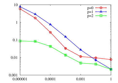
Figure 1: The boundary bias becomes less significant and the gap closes as correlation decreases for estimating the mutual information (left). Local approximation around the blue $*$ in the center. The degree-2 local likelihood approximation (contours in green) automatically captures the local structure whereas the standard $k$-NN approach (uniform distribution in red circle) fails (left).

3 $k$-LNN Entropy Estimator

We consider resubstitution entropy estimators of the form ${\widehat{H}}(x)=-(1/n)\sum_{i=1}^{n}\log\widehat{f}_{n}(X_{i})$ and propose to use the local likelihood density estimator in (7) and a choice of bandwidth that is local (varying for each point $x$) and adaptive (based on the data). Concretely, we choose, for each sample point $X_{i}$, the bandwidth $h_{X_{i}}$ to be the the distance to its $k$-th nearest neighbor $\rho_{k,i}$. Precisely, we propose the following $k$-Local Nearest Neighbor ($k$-LNN) entropy estimator of degree-$2$:

$${\widehat{H}}_{k{\rm LNN}}^{(n)}(X) = -\frac{1}{n}\sum_{i=1}^{n}\left\{\log\frac{S_{0,i}}{n(2\pi)^{d/2}\rho_{k,i}^{d}|\Sigma_{i}|^{1/2}}-\frac{1}{2}\frac{1}{S_{0,i}^{2}}S_{1,i}^{T}\Sigma_{i}^{-1}S_{1,i}\right\}-B_{k,d}\;,$$ (9)

where subtracting $B_{k,d}$ defined in Theorem 1 removes the asymptotic bias, and $k\in{\mathbb{Z}}^{+}$ is the only hyper parameter determining the bandwidth. In practice $k$ is a small integer fixed to be in the range $4\sim 8$. We only use the $\lceil\log n\rceil$ nearest subset of samples ${\cal T}_{i}=\{j\in[n]\,:\,j\neq i\text{ and }\|X_{i}-X_{j}\|\leq\rho_{\lceil\log n\rceil,i}\}$ in computing the quantities below:

$$S_{0,i}\equiv\sum_{j\in{\cal T}_{i,m}}e^{-\frac{\|X_{j}-X_{i}\|^{2}}{2\rho_{k,i}^{2}}}\;,\;\;\;\;S_{1,i}\equiv\sum_{j\in{\cal T}_{i,m}}\frac{1}{\rho_{k,i}}(X_{j}-X_{i})e^{-\frac{\|X_{j}-X_{i}\|^{2}}{2\rho_{k,i}^{2}}}\;,$$

$$S_{2,i}\equiv\sum_{j\in{\cal T}_{i,m}}\frac{1}{\rho_{k,i}^{2}}(X_{j}-X_{i})(X_{j}-X_{i})^{T}e^{-\frac{\|X_{j}-X_{i}\|^{2}}{2\rho_{k,i}^{2}}}\;,\;\;\Sigma_{i}\equiv\frac{S_{0,i}S_{2,i}-S_{1,i}S_{1,i}^{T}}{S_{0,i}^{2}}\;.$$ (10)

The truncation is important for computational efficiency, but the analysis works as long as $m=O(n^{{1/(2d)}-\varepsilon})$ for any positive $\varepsilon$ that can be arbitrarily small. For a larger $m$, for example of $\Omega(n)$, those neighbors that are further away have a different asymptotic behavior. We show in Theorem 1 that the asymptotic bias is independent of the underlying distribution and hence can be precomputed and removed, under mild conditions on a twice continuously differentiable pdf $f(x)$ (cf. Lemma 3.1 below).

Theorem 1.

For $k\geq 3$ and $X_{1},X_{2},\dots,X_{n}\in\mathbb{R}^{d}$ are i.i.d. samples from a twice continuously differentiable pdf $f(x)$, then

$$\lim_{n\to\infty}{\mathbb{E}}[{\widehat{H}}^{(n)}_{k{\rm LNN}}(X)] = H(X)\;,$$ (11)

where $B_{k,d}$ in (9) is a constant that only depends on $k$ and $d$. Further, if ${\mathbb{E}}[(\log f(X))^{2}]<\infty$ then the variance of the proposed estimator is bounded by ${\rm Var}[{\widehat{H}}^{(n)}_{k{\rm LNN}}(X)]=O((\log n)^{2}/n)$.

This proves the $L_{1}$ and $L_{2}$ consistency of the $k$-LNN estimator; we relegate the proof to Section 10 for ease of reading the main part of the paper. The proof assumes Ansatz 1 (also stated in Section 10, which states that a certain exchange of limit holds. As noted in [28], such an assumption is common in the literature on consistency of $k$-NN estimators, where it has been implicitly assumed in existing analyses of entropy estimators including [15, 9, 18, 39], without explicitly stating that such assumptions are being made. Our choice of a local adaptive bandwidth $h_{X_{i}}=\rho_{k,i}$ is crucial in ensuring that the asymptotic bias $B_{k,d}$ does not depend on the underlying distribution $f(x)$. This relies on a fundamental connection to the theory of asymptotic order statistics made precise in Lemma 3.1, which also gives the explicit formula for the bias below.

The main idea is that the empirical quantities used in the estimate (10) converge in large $n$ limit to similar quantities defined over order statistics. We make this intuition precise in the next section. We define order statistics over i.i.d. standard exponential random variables $E_{1},E_{2},\ldots,E_{m}$ and i.i.d. random variables $\xi_{1},\xi_{2},\ldots,\xi_{m}$ drawn uniformly (the Haar measure) over the unit sphere in ${\mathbb{R}}^{d}$, for a variable $m\in{\mathbb{Z}}^{+}$. We define for $\alpha\in\{0,1,2\}$,

$$\tilde{S}^{(m)}_{\alpha}\equiv\sum_{j=1}^{m}\xi_{j}^{(\alpha)}\,\frac{(\sum_{\ell=1}^{j}E_{\ell})^{\alpha}}{(\,\sum_{\ell=1}^{k}E_{\ell}\,)^{\alpha}}\exp\left\{-\frac{(\,\sum_{\ell=1}^{j}E_{\ell}\,)^{2}}{2(\,\sum_{\ell=1}^{k}E_{\ell}\,)^{2}}\right\}\;,$$ (12)

where $\xi_{j}^{(0)}=1$, $\xi_{j}^{(1)}=\xi_{j}\in{\mathbb{R}}^{d}$, and $\xi_{j}^{(2)}=\xi_{j}\xi_{j}^{T}\in{\mathbb{R}}^{d\times d}$, and let ${\tilde{S}}_{\alpha}=\lim_{m\to\infty}{\tilde{S}}_{\alpha}^{(m)}$ and ${\widetilde{\Sigma}}=(1/{\tilde{S}}_{0})^{2}({\tilde{S}}_{0}{\tilde{S}}_{2}-{\tilde{S}}_{1}{\tilde{S}}_{1}^{T})$. We show that the limiting ${\tilde{S}}_{\alpha}$’s are well-defined (in the proof of Theorem 1) and are directly related to the bias terms in the resubstitution estimator of entropy:

$$B_{k,d}={\mathbb{E}}[\,\log(\sum_{\ell=1}^{k}E_{\ell})+\frac{d}{2}\log 2\pi-\log C_{d}-\log{\tilde{S}}_{0}+\frac{1}{2}\log\big{|}{\widetilde{\Sigma}}\big{|}+(\frac{1}{2{\tilde{S}}_{0}^{2}}{\tilde{S}}_{1}^{T}{\widetilde{\Sigma}}^{-1}{\tilde{S}}_{1})\,]\;.$$ (13)

In practice, we propose using a fixed small $k$ such as five. For $k\leq 3$ the estimator has a very large variance, and numerical evaluation of the corresponding bias also converges slowly. For some typical choices of $k$, we provide approximate evaluations below, where $0.0183(\pm 6)$ indicates empirical mean $\mu=183\times 10^{-4}$ with confidence interval $6\times 10^{-4}$. In these numerical evaluations, we truncated the summation at $m=50,000$. Although we prove that $B_{k,d}$ converges in $m$, in practice, one can choose $m$ based on the number of samples and $B_{k,d}$ can be evaluated for that $m$.

Theoretical contribution: Our key technical innovation is a fundamental connection between nearest neighbor statistics and asymptotic order statistics, stated below as Lemma 3.1: we show that the (normalized) distances $\rho_{\ell,i}$’s jointly converge to the standardized uniform order statistics and the directions $(X_{j_{\ell}}-X_{i})/\|X_{j_{\ell}}-X_{i}\|$’s converge to independent uniform distribution (Haar measure) over the unit sphere.

		$k$
		$4$	$5$	$6$	$7$	$8$	$9$
$d$	$1$	-0.0183($\pm$6)	-0.0233($\pm$6)	-0.0220($\pm$4)	-0.0200($\pm$4)	-0.0181($\pm$4)	-0.0171($\pm$3)
	$2$	-0.1023($\pm$5)	-0.0765($\pm$4)	-0.0628($\pm$4)	-0.0528($\pm$3)	-0.0448($\pm$3)	-0.0401($\pm$3)

Table 1: Numerical evaluation of $B_{k,d}$, via sampling $1,000,000$ instances for each pair $(k,d)$.

Conditioned on $X_{i}=x$, the proposed estimator uses nearest neighbor statistics on $Z_{\ell,i}\equiv X_{j_{\ell}}-x$ where $X_{j_{\ell}}$ is the $\ell$-th nearest neighbor from $x$ such that $Z_{\ell,i}=((X_{j_{\ell}}-X_{i})/\|X_{j_{\ell}}-X_{i}\|)\rho_{\ell,i}$. Naturally, all the techniques we develop in this paper generalize to any estimators that depend on the nearest neighbor statistics $\{Z_{\ell,i}\}_{i,\ell\in[n]}$ – and the value of such a general result is demonstrated later (in Section 4) when we evaluate the bias in similarly inspired entropy estimators [6, 7, 22, 15].

Lemma 3.1.

Let $E_{1},E_{2},\dots,E_{m}$ be i.i.d. standard exponential random variables and $\xi_{1},\xi_{2},\dots,\xi_{m}$ be i.i.d. random variables drawn uniformly over the unit $(d-1)$-dimensional sphere in $d$ dimensions, independent of the $E_{i}$’s. Suppose $f$ is twice continuously differentiable and $x\in\mathbb{R}^{d}$ satisfies that there exists $\varepsilon>0$ such that $f(a)>0$, $\|\nabla f(a)\|=O(1)$ and $\|H_{f}(a)\|=O(1)$ for any $\|a-x\|<\varepsilon$. Then for any $m=O(\log n)$, we have the following convergence conditioned on $X_{i}=x$:

$$\lim_{n\to\infty}d_{\rm TV}((c_{d}nf(x))^{1/d}(\,Z_{1,i},\dots,Z_{m,i}\,)\;,\;(\,\xi_{1}E_{1}^{1/d},\dots,\xi_{m}(\sum_{\ell=1}^{m}E_{\ell})^{1/d}\,))=0\;.$$ (14)

where $d_{\rm TV}(\cdot,\cdot)$ is the total variation and $c_{d}$ is the volume of unit Euclidean ball in $\mathbb{R}^{d}$.

Empirical contribution: Numerical experiments suggest that the proposed estimator outperforms state-of-the-art entropy estimators, and the gap increases with correlation. The idea of using $k$-NN distance as bandwidth for entropy estimation was originally proposed by Kozachenko and Leonenko in [15], and is a special case of the $k$-LNN method we propose with degree $0$ and a step kernel. We refer to Section 4 for a formal comparison. Another popular resubstitution entropy estimator is to use KDE in (3) [13], which is a special case of the $k$-LNN method with degree $0$, and the Gaussian kernel is used in simulations. As comparison, we also study a new estimator [14] based on von Mises expansion (as opposed to simple re-substitution) which has an improved convergence rate in the large sample regime. In Figure 2 (left), we draw $100$ samples i.i.d. from two standard Gaussian random variables with correlation $r$, and plot resulting mean squared error averaged over $100$ instances. The ground truth, in this case is $H(X)=\log(2\pi e)+0.5\log(1-r^{2})$. On the right, we repeat the same simulation for fixed $r=0.99999$ and varying number of samples and $m=7\log_{e}n$.

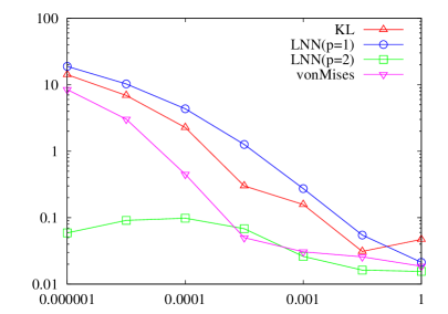
Figure 2: Degree-2 $k$-LNN outperforms other state-of-the-art estimators for entropy estimation.

In Figure 3, we repeat the same simulation for 6 standard Gaussian random variables with ${\rm Cov}(X_{1},X_{2})={\rm Cov}(X_{3},X_{4})={\rm Cov}(X_{5},X_{6})=r$ and ${\rm Cov}(X_{i},X_{j})=0$ for other pairs $(i,j)$. On the left, we draw $100$ i.i.d. samples with various $r$. We plot resulting mean squared error averaged over $100$ instances. The ground truth is $H(X)=3\log(2\pi e)+1.5\log(1-r^{2})$. On the right, we repeat the same simulation for fixed $r=0.99999$ and varying number of samples and $m=7\log_{e}n$.

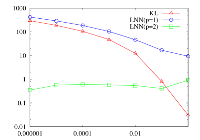
Figure 3: Degree-2 $k$-LNN outperforms other state-of-the-art estimators for high-dimensional entropy estimation.

In Figure 4 (left), we draw $100$ samples i.i.d. from a mixture of two joint Gaussian distributions with zero mean and covariance $\begin{pmatrix}1&r\\ r&1\end{pmatrix}$ and $\begin{pmatrix}1&-r\\ -r&1\end{pmatrix}$, respectively, and plot resulting average estimate over $100$ instances. Here we plot an upper bound of the ground truth $H(X)\leq\log(2)+\log(2\pi e)+0.5\log(1-r^{2})$ for $r\geq 0.9$. On the right, we repeat the same simulation for fixed $r=0.99999$ and varying number of samples and $m=7\log_{e}n$.

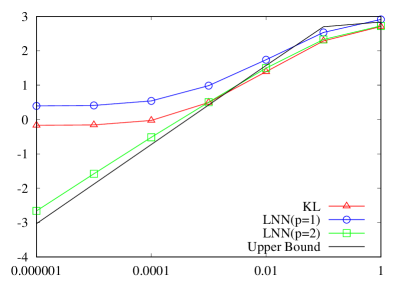
Figure 4: Degree-2 $k$-LNN outperforms other state-of-the-art estimators for non-Gaussian entropy estimation.

4 Universality of the $k$-LNN approach

In this section, we show that Theorem 1 holds universally for a general family of entropy estimators, specified by the choice of $k\in{\mathbb{Z}}^{+}$, degree $p\in{\mathbb{Z}}^{+}$, and a kernel $K:{\mathbb{R}}^{d}\to{\mathbb{R}}$, thus allowing a unified view of several seemingly disparate entropy estimators [15, 6, 7, 22]. The template of the entropy estimator is the following: given $n$ i.i.d. samples, we first compute the local density estimate by maximizing the local likelihood (1) with bandwidth $\rho_{k,i}$, and then resubstitute it to estimate entropy: ${\widehat{H}}_{k,p,K}^{(n)}(X)=-(1/n)\sum_{i=1}^{n}\log\widehat{f}_{n}(X_{i})$.

Theorem 2.

For the family of estimators described above, under the hypotheses of Theorem 1, if the solution to the maximization $\widehat{a}(x)=\arg\max_{a}{\cal L}_{x}(f_{a,x})$ exists for all $x\in\{X_{1},\ldots,X_{n}\}$, then for any choice of $k\geq p+1$, $p\in{\mathbb{Z}}^{+}$, and $K:{\mathbb{R}}^{d}\to{\mathbb{R}}$, the asymptotic bias is independent of the underlying distribution:

$$\lim_{n\to\infty}{\mathbb{E}}[{\widehat{H}}^{(n)}_{k,p,K}(X)] = H(X)+{\widetilde{B}}_{k,p,K,d}\;,$$ (15)

for some constant ${\widetilde{B}}_{k,d,p,K}$ that only depends on $k,p,K$ and $d$.

We provide a proof in Section 11. Although in general there is no simple analytical characterization of the asymptotic bias ${\widetilde{B}}_{k,p,K,d}$ it can be readily numerically computed: since ${\widetilde{B}}_{k,p,K,d}$ is independent of the underlying distribution, one can run the estimator over i.i.d. samples from any distribution and numerically approximate the bias for any choice of the parameters. However, when the maximization $\widehat{a}(x)=\arg\max_{a}{\cal L}_{x}(f_{a,x})$ admits a closed form solution, as is the case with proposed $k$-LNN, then $\widetilde{B}_{k,p,K,d}$ can be characterized explicitly in terms of uniform order statistics.

This family of estimators is general: for instance, the popular KL estimator is a special case with $p=0$ and a step kernel $K(u)={\mathbb{I}}(\|u\|\leq 1)$. [15] showed (in a remarkable result at the time) that the asymptotic bias is independent of the dimension $d$ and can be computed exactly to be $\log n-\psi(n)+\psi(k)-\log k$ and $\psi(k)$ is the digamma function defined as $\psi(x)=\Gamma^{-1}(x)d\Gamma(x)/dx$. The dimension independent nature of this asymptotic bias term (of $O(n^{-1/2})$ for $d=1$ in [36, Theorem 1] and $O(n^{-1/d})$ for general $d$ in [8]) is special to the choice of $p=0$ and the step kernel; we explain this in detail in Section 11, later in the paper. Analogously, the estimator in [6] can be viewed as a special case with $p=0$ and an ellipsoidal step kernel.

5 $k$-LNN Mutual information estimator

Given an entropy estimator ${\widehat{H}}_{\rm KL}$, mutual information can be estimated: ${\widehat{I}}_{\rm 3KL}={\widehat{H}}_{\rm KL}(X)+{\widehat{H}}_{\rm KL}(Y)-{\widehat{H}}_{\rm KL}(X,Y)$. In [16], Kraskov and Stögbauer and Grassberger introduced ${\widehat{I}}_{\rm KSG}(X;Y)$ by coupling the choices of the bandwidths. The joint entropy is estimated in the usual way, but for the marginal entropy, instead of using $k$NN distances from $\{X_{j}\}$, the bandwidth $h_{X_{i}}=\rho_{k,i}(X,Y)$ is chosen, which is the $k$ nearest neighbor distance from $(X_{i},Y_{i})$ for the joint data $\{(X_{j},Y_{j})\}$. Consider ${\widehat{I}}_{\rm 3LNN}(X;Y)={\widehat{H}}_{k{\rm LNN}}(X)+{\widehat{H}}_{k{\rm LNN}}(Y)-{\widehat{H}}_{k{\rm LNN}}(X,Y)$. Inspired by [16], we introduce the following novel mutual information estimator we denote by ${\widehat{I}}_{\rm LNN-KSG}(X;Y)$. where for the joint $(X,Y)$ we use the LNN entropy estimator we proposed in (9), and for the marginal entropy we use the bandwidth $h_{X_{i}}=\rho_{k,i}(X,Y)$ coupled to the joint estimator. Empirically, we observe ${\widehat{I}}_{\rm KSG}$ outperforms ${\widehat{I}}_{\rm 3KL}$ everywhere, validating the use of correlated bandwidths. However, the performance of ${\widehat{I}}_{{\rm LNN-KSG}}$ is similar to ${\widehat{I}}_{3{\rm LNN}}$–sometimes better and sometimes worse.

In Figure 5 (left), we estimate mutual information under the same setting as in Figure 2 (left). For most regimes of correlation $r$, both 3LNN and LNN-KSG outperforms other state-of-the-art estimators. The gap increases with correlation $r$. On the right, we draw i.i.d. samples from two random variables $X$ and $Y$, where $X$ is uniform over $[0,1]$ and $Y=X+U$, where $U$ is uniform over $[0,0.01]$ independent of $X$. In the large sample limit, all estimators find the correct mutual information. The plot show how sensitive the estimates are, in the small sample regime. Both LNN and LNN-KSG are significantly more robust compared to other approaches. Mutual information estimators have been recently proposed in [6, 7, 22] based on local likelihood maximization. However, they involve heuristic choices of hyper-parameters or solving elaborate optimization and numerical integrations, which are far from being easy to implement.

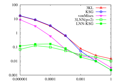
Figure 5: Proposed ${\widehat{I}}_{\rm LNN-KSG}$ and ${\widehat{I}}_{\rm 3LNN}$ outperform other state-of-the-art estimators.

In Figure 6, we test the mutual information estimators for $Y=f(X)+U$, where $X$ is uniformly distributed over $[0,1]$ and $U$ is uniformly distributed over $[0,\theta]$, independent of $X$, for some noise level $\theta$. Similar simulation were studied in [7]. We draw 2500 i.i.d. sample points for each relationship. The plot show that for small noise level $\theta$, i.e., near-functional related random variables, our proposed estimators ${\widehat{I}}_{3LNN}$ and ${\widehat{I}}_{LNN-KSG}$ perform much better than 3KL and KSG estimators. Also our proposed estimators can handle both linear and nonlinear functional relationships.

$\begin{array}[]{lll}\includegraphics[width=140.92792pt]{linear}&\includegraphics[width=140.92792pt]{quadratic}&\includegraphics[width=140.92792pt]{cubic}\put(-490.0,50.0){${\mathbb{E}}[{\widehat{I}}(X;Y)]$}\put(-400.0,100.0){$Y=X+U$}\put(-250.0,100.0){$Y=X^{2}+U$}\put(-100.0,100.0){$Y=X^{3}+U$}\end{array}$

$\begin{array}[]{lll}\includegraphics[width=140.92792pt]{exponential}&\includegraphics[width=140.92792pt]{sin}&\includegraphics[width=140.92792pt]{cos}\put(-490.0,50.0){${\mathbb{E}}[{\widehat{I}}(X;Y)]$}\put(-400.0,100.0){$Y=2^{X}+U$}\put(-260.0,100.0){$Y=\sin(4\pi X)+U$}\put(-120.0,100.0){$Y=\cos(5\pi X(1-X))+U$}\put(-400.0,-10.0){Noise Level $\theta$}\put(-250.0,-10.0){Noise Level $\theta$}\put(-100.0,-10.0){Noise Level $\theta$}\end{array}$

Figure 6: Functional relationship test for mutual information estimators. Proposed ${\widehat{I}}_{\rm LNN-KSG}$ and ${\widehat{I}}_{\rm 3LNN}$ outperform other state-of-the-art estimators.

In Figure 7, we test our estimators on linear and nonlinear relationships for both low-dimensional ($D=2$) and high-dimensional ($D=5$). Here $X_{i}$’s are uniformly distributed over $[0,1]$ and $U$ is uniformly distributed over $[-3^{8}/2,3^{8}/2]$, independently of $X_{i}$’s. Similar simulation were studied in [6]. We can see that our estimators ${\widehat{I}}_{3LNN}$ and ${\widehat{I}}_{LNN-KSG}$ converges much faster than $\hat{I}_{3KL}$ and ${\widehat{I}}_{KSG}$.

$\begin{array}[]{ll}\includegraphics[width=187.89912pt]{2d_linear}&\includegraphics[width=187.89912pt]{2d_quadratic}\put(-425.0,70.0){${\mathbb{E}}[{\widehat{I}}(X;Y)]$}\put(-320.0,130.0){$Y=X_{1}+U$}\put(-120.0,130.0){$Y=X_{1}^{2}+U$}\end{array}$

$\begin{array}[]{ll}\includegraphics[width=187.89912pt]{5d_linear}&\includegraphics[width=187.89912pt]{5d_quadratic}\put(-425.0,70.0){${\mathbb{E}}[{\widehat{I}}(X;Y)]$}\put(-350.0,130.0){$Y=X_{1}+X_{2}+X_{3}+X_{4}+U$}\put(-150.0,130.0){$Y=X_{1}^{2}+X_{2}^{2}+X_{3}^{2}+X_{4}^{2}+U$}\put(-330.0,-10.0){number of samples}\put(-130.0,-10.0){number of samples}\end{array}$

Figure 7: Estimated Mutual Information of low/high-dimensional relationships

6 Breaking the bandwidth barrier

While $k$-NN distance based bandwidth are routine in practical usage [31], the main finding of this work is that they also turn out to be the “correct" mathematical choice for the purpose of asymptotically unbiased estimation of an integral functional such as the entropy: $-\int f(x)\log f(x)$; we briefly discuss the ramifications below. Traditionally, when the goal is to estimate $f(x)$, it is well known that the bandwidth should satisfy $h\to 0$ and $nh^{d}\to\infty$, for KDEs to be consistent. As a rule of thumb, $h=1.06\widehat{\sigma}n^{-1/5}$ is suggested when $d=1$ where $\widehat{\sigma}$ is the sample standard deviation [41, Chapter 6.3]. On the other hand, when estimating entropy, as well as other integral functionals, it is known that resubstitution estimators of the form $-(1/n)\sum_{i=1}^{n}\log\widehat{f}(X_{i})$ achieve variances scaling as $O(1/n)$ independent of the bandwidth [19]. This allows for a bandwidth as small as $O(n^{-1/d})$.

The bottleneck in choosing such a small bandwidth is the bias, scaling as $O(h^{2}+(nh^{d})^{-1}+E_{n})$ [19], where the lower order dependence on $n$, dubbed $E_{n}$, is generally not known. The barrier in choosing a global bandwidth of $h=O(n^{-1/d})$ is the strictly positive bias whose value depends on the unknown distribution and cannot be subtracted off. However, perhaps surprisingly, the proposed local and adaptive choice of the $k$-NN distance admits an asymptotic bias that is independent of the unknown underlying distribution. Manually subtracting off the non-vanishing bias gives an asymptotically unbiased estimator, with a potentially faster convergence as numerically compared below. Figure 8 illustrates how $k$-NN based bandwidth significantly improves upon, say a rule-of-thumb choice of $O(n^{-1/(d+4)})$ explained above and another choice of $O(n^{-1/(d+2)})$. In the left figure, we use the setting from Figure 2 (right) but with correlation $r=0.999$. On the right, we generate $X\sim{\cal N}(0,1)$ and $U$ from uniform $[0,0.01]$ and let $Y=X+U$ and estimate $I(X;Y)$. Following recent advances in [18, 33], the proposed local estimator has a potential to be extended to, for example, Renyi entropy, but with a multiplicative bias as opposed to additive.

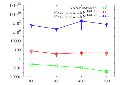
Figure 8: Local and adaptive bandwidth significantly improves over rule-of-thumb fixed bandwidth.

7 Discussion

The topic of estimation of an integral functional of an unknown density from i.i.d. samples is a classical one in statistics and we tie together a few pertinent topics from the literature in the context of the results of this manuscript.

7.1 Uniform order statistics and NN distances

The expression for the asymptotic bias in (13) which is independent of the underlying distribution forms the main result of this paper and crucially depends on Lemma 3.1. Precisely, the lemma implies that the quantities $S_{i}$’s in (10) converge in distribution to ${\tilde{S}}_{i}$’s in (12). There are two parts to this convergence result: the nearest neighbor distances converge to uniform order statistics and the directions to those nearest neighbors converge independently to Haar measures on the unit sphere. The former has been extensively studied, for example see [29] for a survey of results. The latter is a new result that we state in Lemma 3.1, and proved in Section 9. Intuitively, assuming smoothness, the probability density $f_{X}$ in the neighborhood of a sample $X_{i}$ (as defined by the distance to the $k$-th nearest neighbor) converges to a uniform distribution over a ball (of radius decreasing at the rate $\rho_{k,i}=\Theta(n^{-1/d})$), as more samples are collected. The nearest neighbor distances and directions converge to those from the uniform distribution over the ball, and Lemma 3.1 makes this intuition precise for the nearest $m$ neighbors up to $m=O(n^{1/(2d)-\epsilon})$ with any arbitrarily small but positive $\varepsilon$.

Only the convergence analysis of the distances, and not the directions, is required for traditional $k$-NN based estimators, such as the entropy estimator of [15]. In the seminal paper, [15] introduced resubstitution entropy estimators of the form ${\widehat{H}}(X)=-(1/n)\sum_{i=1}^{n}\log\widehat{f}_{n}(X_{i})$ with $\widehat{f}_{n}(x)={k}/(n\,C_{d}\,\rho_{k,x}^{d})$ (as defined in (4)). This $k$-NN estimator has a non-vanishing asymptotic bias, which was computed as $B_{k,d}=(\psi(k)-\log(k))$ with the digamma function $\psi(\cdot)$ and was suggested to be manually removed. For $k=1$ this was proved in the original paper of [15], which later was extended in [32, 9] to general $k$. This mysterious bias term $B_{k,d}=(\psi(k)-\log(k))$ whose original proofs in [15, 32, 9] provided little explanation for, can be alternatively proved with both rigor and intuition by making connections to uniform order statistics. For a special case of $k=1$, with extra assumptions on the support being compact, such an elegant proof is provided in [2, Theorem 7.1] which explicitly applies the convergence of the nearest neighbor distance to uniform order statistics. Namely,

$${\mathbb{E}}[\widehat{H}(X)] = {\mathbb{E}}\Big{[}\,-\frac{1}{n}\sum_{i=1}^{n}\log\Big{(}\frac{k}{n\,C_{d}\,\rho_{k,X_{i}}^{d}}\Big{)}\,\Big{]}$$

$$\to {\mathbb{E}}\Big{[}-\log\frac{k\,f(X_{i})}{\sum_{j=1}^{k}E_{j}}\Big{]}$$

$$= H(X)+\psi(k)-\log(k)\;,$$

where the asymptotic expression follows from $C_{d}\,n\,f(x)\rho_{k,x}^{d}\to\sum_{j=1}^{k}E_{j}$ as shown, for example, in Lemma 3.1 and we used ${\mathbb{E}}[\log\sum_{j=1}^{k}E_{j}]=\psi(k)$, where $\psi(k)=$ is the digamma function defined as $\psi(x)=\Gamma^{-1}(x)d\Gamma(x)/dx$ and for large $x$ it is approximately $\log(x)$ up to $O(1/x)$, i.e. $\psi(x)=\log x-1/(2x)+o(1/x)$. Note that this only requires the convergence of the distance and not the direction. Inspired by this modern approach, we extend such a connection in Lemma 3.1 to prove consistency of our estimator.

7.2 Convergence rate of the bias

Establishing the convergence rate of the KL estimator is a challenging problem, and is not quite resolved despite work over the past three decades. The $O(1/n)$ convergence rate of the variance is established in [3, 18, 2, 4] under various assumptions. Establishing the convergence rate of the bias is more challenging. It has been first studied in [10, 11], where root-$n$ consistency is shown in 1-dimension with bounded support and assuming $f(x)$ is bounded below. [36] is the first to prove a root mean squared error convergence rate of $O(1/\sqrt{n})$ for general densities with unbounded support in 1-dimension and exponentially decaying tail, such as the Gaussian density. These assumptions are relaxed in [5], where zeroes and fat tails are allowed in $f(x)$. In general $d$-dimensions, [8, 33] prove bounds on the convergence rate of the bias for finite $k=O(1)$, and [24, 1] for $k=\Omega(\log n)$. Establishing the convergence rate for the bias of the proposed local estimator is an interesting open problem – it is interesting to see if the superior empirical performance of the local estimator is captured in the asymptotics of rate of convergence of the bias.

It is intuitive that kernel density estimators can capture the structure in the distribution if the distribution lies on a lower dimensional manifold. This is made precise in [27], which also shows improved convergence rates for distributions whose support is on low dimensional manifolds. However, the estimator in [27] critically uses the geodesic distances between the sample points on the manifold. Given that the proposed estimators fit distributions locally, a concrete question of interest is whether such an improvement can be achieved without such an explicit knowledge of the geodesic distances, i.e., whether the local estimators automatically adapt to underlying lower dimensional structures.

7.3 Ensemble estimators

Recent works [34, 25, 26, 1] have proposed ensemble estimators, which use known estimators based on kernel density estimators and $k$-NN methods and construct a new estimate by taking the weighted linear combination of those methods with varying bandwidth or $k$, respectively. With a proper choice of the weights, which can be computed analytically by solving a simple linear program, a boosting of the convergence rate can be achieved. The key property that allows the design of such ensemble estimators is that the leading terms (in terms of the sample size $n$) of the bias have a multiplicative constant that only depends on the unknown distribution. An intuitive explanation for this phenomenon is provided in [1] in the context of $k$-NN methods; it is interesting to explore if such a phenomenon continues in the $k$-LNN scenario studied in this paper. Such a study would potentially lead to ensemble-based estimators in the local setting and also naturally allow a careful understanding of the rate of convergence of the bias term.

8 Proofs

8.1 Proof of proposition 2.1

We first prove the derivation of the LLDE with degree $p=2$ in Equation (7). The gradient of the local likelihood evaluated at the maximizer is zero [21], which gives a computational tool for finding the maximizer:

$$\frac{1}{n}\sum_{j=1}^{n}K(\frac{X_{j}-x}{h})=\int K(\frac{u-x}{h})e^{a_{0}+a_{1}^{T}(u-x)+(u-x)^{T}a_{2}(u-x)}du\;,$$ (16)

$$\frac{1}{n}\sum_{j=1}^{n}\frac{X_{j}-x}{h}K(\frac{X_{j}-x}{h})=\int\frac{u-x}{h}K(\frac{u-x}{h})e^{a_{0}+a_{1}^{T}(u-x)+(u-x)^{T}a_{2}(u-x)}du\;,$$ (17)

$$\frac{1}{n}\sum_{j=1}^{n}\frac{(X_{j}-x)(X_{j}-x)^{T}}{h^{2}}K(\frac{X_{j}-x}{h})$$

$$\;\;\;\;=\int\frac{(u-x)(u-x)^{T}}{h^{2}}K(\frac{u-x}{h})e^{a_{0}+a_{1}^{T}(u-x)+(u-x)^{T}a_{2}(u-x)}du\;,$$ (18)

where $K(x)=\exp\{-\|x\|^{2}/2\}$ is the Gaussian kernel. Notice that the left-hand side of the equations are $S_{0}/n$, $S_{1}/n$ and $S_{2}/n$, respectively. The RHS can be written in closed forms as:

$$\frac{1}{n}S_{0} = (2\pi)^{d/2}|{M}|^{-1/2}e^{a_{0}+\frac{1}{2}a_{1}^{T}M^{-1}a_{1}}\;,$$ (19)

$$\frac{1}{n}S_{1} = \frac{1}{nh}S_{0}M^{-1}a_{1}\;,$$ (20)

$$\frac{1}{n}S_{2} = \frac{1}{nh^{2}}S_{0}(M^{-1}+M^{-1}a_{1}a_{1}^{T}M^{-1})\;,$$ (21)

where $M=h^{-2}I_{d\times d}-2a_{2}$ assuming $h$ sufficiently small such that $M$ is positive definite. We want to derive $\hat{f}(x)=\exp\{a_{0}\}$ from the equations. From (20) we get $M^{-1}a_{1}=S_{1}(h/S_{0})$. Together with (21), we get $M^{-1}+M^{-1}a_{1}a_{1}^{T}M^{-1}=S_{2}(h^{2}/S_{0})$. Hence, $M^{-1}=(S_{2}/S_{0}-(S_{1}/S_{0})(S_{1}/S_{0})^{T})h^{2}=h^{2}\Sigma$. Plug them in (19), we obtain the desired expression.

Analogously, for the derivation of the LLDE with degree $p=1$ in Equation (5), we get

$$\frac{1}{n}S_{0} = (2\pi)^{d/2}h^{d}e^{a_{0}+\frac{h^{2}}{2}a_{1}^{T}a_{1}}\;,$$ (22)

$$\frac{1}{n}S_{1} = \frac{h}{n}S_{0}a_{1}\;.$$ (23)

This gives $a_{1}=(1/(hS_{0}))S_{1}$, and $e^{a_{0}}=(S_{0}/(n(2\pi)^{d/2}h^{d}))\,\exp\{-0.5\|S_{1}\|^{2}/S_{0}^{2}\}$.

9 Proof of Lemma 3.1

Let us introduce some notations first. Define $S^{d-1}\equiv\{x\in\mathbb{R}^{d}:\|x\|=1\}$ as the unit $(d-1)$-dimensional sphere and $\sigma^{d-1}$ as a normalized spherical measure on $S^{d-1}$. For any $\theta=(\theta_{1},\dots,\theta_{m})\in(S^{d-1})^{m}$ and $x=(x_{1},\dots,x_{m})\in\mathbb{R}_{+}^{m}$, define $\theta x\equiv(\theta_{1}x_{1},\dots,\theta_{m}x_{m})\in\mathbb{R}^{d\times m}$. For any set $B\in\mathbb{R}^{d\times m}$ and $\theta\in(S^{d-1})^{m}$, define $B_{\theta}=\{x\in\mathbb{R}_{+}^{m}:\theta x\in B\}$. Let $\{\xi_{i}\}_{i=1}^{m}$ be i.i.d. random variables uniformly over $S^{d-1}$. Then for any joint random variables $(W_{1},\dots,W_{m})\in\mathbb{R}_{+}^{m}$ which are independent with $\{\xi_{i}\}_{i=1}^{m}$, we have

$${\mathbb{P}}\{(\xi_{1}W_{1},\dots,\xi_{m}W_{m})\in B\} = \int_{\theta\in(S^{d-1})^{m}}{\mathbb{P}}\{(W_{1},\dots,W_{m})\in B_{\theta}\,|\,\theta\}\,d(\sigma^{d-1})^{m}(\theta)\;.$$ (24)

Let $Z=(Z_{1,i},\ldots,Z_{m,i})$, $\|Z\|=(\|Z_{1,i}\|,\ldots,\|Z_{m,i}\|)$ and let $E=(E_{1}^{1/d},\ldots,(\sum_{\ell=1}^{m}E_{\ell})^{1/d})$, then

$$\left|\,{\mathbb{P}}\left\{\,(c_{d}nf(x))^{1/d}Z\in B\,\right\}-{\mathbb{P}}\left\{\,\left(\,\xi_{1}E_{1}^{1/d},\dots,\xi_{m}(\sum_{\ell=1}^{m}E_{\ell})^{1/d}\,\right)\in B\,\right\}\,\right|\,$$ (25)

$$\leq \left|\,{\mathbb{P}}\left\{\,(c_{d}nf(x))^{1/d}Z\in B\,\right\}-\int_{\theta\in(S^{d-1})^{m}}{\mathbb{P}}\{(E_{1}^{1/d},\dots,(\sum_{\ell=1}^{m}E_{\ell})^{1/d})\in B_{\theta}\,|\,\theta\}\,d(\sigma^{d-1})^{m}(\theta)\,\right|\,$$

$$\leq \left|\,{\mathbb{P}}\left\{\,(c_{d}nf(x))^{1/d}Z\in B\,\right\}-\int_{\theta\in(S^{d-1})^{m}}{\mathbb{P}}\{(c_{d}nf(x))^{1/d}\|Z\|\in B_{\theta}\,|\,\theta\}\,d(\sigma^{d-1})^{m}(\theta)\,\right|\,$$

$$+ \int_{\theta\in(S^{d-1})^{m}}\left|\,{\mathbb{P}}\{(c_{d}nf(x))^{1/d}\|Z\|\in B_{\theta}\,|\,\theta\}-{\mathbb{P}}\{E\in B_{\theta}\,|\,\theta\}\,\right|d(\sigma^{d-1})^{m}(\theta)\;.$$

Now consider the first term in (25). We consider two cases separately.

Case 1. If $\|Z_{m,i}\|\geq(\sqrt{n}c_{d}f(x))^{-1/d}$, we show that the tail events happen with a low probability. Denote $B(x,r)=\{z:\|z-x\|\leq r\}$ and let $p={\mathbb{P}}\{t\in B(x,\|Z_{m,i}\|)\}=\int_{B(x,\|Z_{m,i}\|)}f(t)dt$. Since $f$ is twice continuously differentiable, we can see that $p\geq 0.5c_{d}\|Z_{m,i}\|^{d}f(x)\geq 0.5/\sqrt{n}$ for sufficiently large $n$. Therefore,

$${\mathbb{P}}\{\|Z_{m,i}\|\geq(\sqrt{n}c_{d}f(x))^{-1/d}\} = \sum_{\ell=0}^{m-1}{n\choose\ell}p^{\ell}(1-p)^{n-\ell}\leq\sum_{\ell=0}^{m-1}n^{\ell}\Big{(}1-\frac{1}{2\sqrt{n}}\Big{)}^{(n-\ell)}\,$$ (26)

$$\leq \sum_{\ell=0}^{m-1}n^{l}e^{-(\sqrt{n}-\ell\sqrt{n})/2}\leq mn^{m}e^{-(\sqrt{n}-m/\sqrt{n})/2}\;.$$

Case 2. If $\|Z_{m,i}\|<(\sqrt{n}c_{d}f(x))^{-1/d}$, let $\overline{B}=\{t:(c_{d}nf(x))^{1/d}t\in B\textrm{ and }\|t_{m}\|<(\sqrt{n}c_{d}f(x))^{-1/d}\}$ and $\overline{B_{\theta}}=\{t:(c_{d}nf(x))^{1/d}t\in B_{\theta}\textrm{ and }t_{m}<(\sqrt{n}c_{d}f(x))^{-1/d}\}$. Note that

$${\mathbb{P}}(Z\in{\widetilde{A}})=(n!/(n-k)!)\int_{t\in{\widetilde{A}}}\prod_{j=1}^{m}f(x+t_{j}){\mathbb{P}}_{X}(|X-x|>|t_{m}|)^{n-m}dt\;,$$ (27)

which gives

$$\frac{\int_{\theta\in(S^{d-1})^{m}}{\mathbb{P}}\{(c_{d}nf(x))^{1/d}\|Z\|\in B_{\theta},\|Z_{m,i}\|<(\sqrt{n}c_{d}f(x))^{-1/d}\,|\,\theta\}\,d(\sigma^{d-1})^{m}(\theta)}{{\mathbb{P}}\{(c_{d}nf(x))^{1/d}Z\in B,\|Z_{m,i}\|<(\sqrt{n}c_{d}f(x))^{-1/d}\}}\,$$ (28)

$$= \frac{\int_{\theta\in(S^{d-1})^{m}}{\mathbb{P}}\{\|Z\|\in\overline{B_{\theta}}\,|\,\theta\}\,d(\sigma^{d-1})^{m}(\theta)}{{\mathbb{P}}\{Z\in\overline{B}\}}\,$$

$$= \frac{\int_{\theta\in(S^{d-1})^{m}}\frac{n!}{(n-k)!}\left(\,\int_{t\in\overline{B_{\theta}}}\left(\,\prod_{j=1}^{m}f(x+\theta_{j}t_{j})\,\right)\,\left(\,{\mathbb{P}}\{\|X-x\|>\|t_{m}\|\}\,\right)^{n-m}dt\,\right)\,d(\sigma^{d-1})^{m}(\theta)}{\frac{n!}{(n-k)!}\int_{t\in\overline{B}}\left(\,\prod_{j=1}^{m}f(x+t_{j})\,\right)\,\left(\,{\mathbb{P}}\{\|X-x\|>\|t_{m}\|\}\,\right)^{n-m}dt}\,$$

$$\leq \frac{\sup_{\theta\in(S^{d-1})^{m}}\sup_{t\in\overline{B_{\theta}}}\prod_{j=1}^{m}f(x+\theta_{j}t_{j})}{\inf_{t\in\overline{B}}\prod_{j=1}^{m}f(x+t_{j})}\,$$

$$\leq \left(\,\frac{\sup_{\|t\|\leq(\sqrt{n}c_{d}f(x))^{-1/d}}f(x+t)}{\inf_{\|t\|\leq(\sqrt{n}c_{d}f(x))^{-1/d}}f(x+t)}\,\right)^{m}\;,$$

where the first inequality follows from the fact that $\int_{\theta\in(S^{d-1})^{m}}(\int_{\overline{B_{\theta}}}g(t_{m})dt)d(\sigma^{d-1})^{m}(\theta)=\int_{\overline{B}}g(\|t_{m}\|)dt$. Since $f$ is continuously differentiable, by mean value theorem, there exists $a,b\in B(x,(\sqrt{n}c_{d}f(x))^{-1/d})$ such that

$$\frac{\sup_{\|t\|\leq(\sqrt{n}c_{d}f(x))^{-1/d}}f(x+t)}{\inf_{\|t\|\leq(\sqrt{n}c_{d}f(x))^{-1/d}}f(x+t)} = \frac{f(b)+(a-b)^{T}\nabla f(a)}{f(b)}\leq 1+\frac{2(\sqrt{n}c_{d}f(x))^{-1/d}\|\nabla f(a)\|}{f(b)}\;,$$ (29)

By the assumption, there exists a ball $B(x,\varepsilon)$ such that $\|\nabla f(a)\|=O(1)$ and $f(a)>0$ for all $a\in B(x,\varepsilon)$, so for sufficiently large $n$ such that $(\sqrt{n}c_{d}f(x))^{-1/d}<\varepsilon$, there exists some constant $C$ such that $\sup_{\|t\|\leq(\sqrt{n}c_{d}f(x))^{-1/d}}f(x+t)\leq(1+Cn^{-1/(2d)})\inf_{\|t\|\leq(\sqrt{n}c_{d}f(x))^{-1/d}}f(x+t)$. Therefore, (28) is upper bounded by $(1+Cn^{-1/(2d)})^{m}$. Similarly, (28) is lower bounded by $(1-Cn^{-1/(2d)})^{m}$.

For simplicity, let $\mathcal{E}=\{\|Z_{m,i}\|<(\sqrt{n}c_{d}f(x))^{-1/d}\}$. Then combining the two cases, the first term in (25) is bounded by:

$$\left|\,{\mathbb{P}}\left\{\,(c_{d}nf(x))^{1/d}Z\in B\,\right\}-\int_{\theta\in(S^{d-1})^{m}}{\mathbb{P}}\{(c_{d}nf(x))^{1/d}\|Z\|\in B_{\theta}\,|\,\theta\}\,d(\sigma^{d-1})^{m}(\theta)\,\right|\,$$ (30)

$$\leq {\mathbb{P}}\left\{\,(c_{d}nf(x))^{1/d}Z\in B,\mathcal{E}^{C}\,\right\}+\int_{\theta\in(S^{d-1})^{m}}{\mathbb{P}}\{(c_{d}nf(x))^{1/d}\|Z\|\in B_{\theta},\mathcal{E}^{C}\,|\,\theta\}\,d(\sigma^{d-1})^{m}(\theta)\,$$

$$+ \left|\,{\mathbb{P}}\left\{\,(c_{d}nf(x))^{1/d}Z\in B,\mathcal{E}\,\right\}-\int_{\theta\in(S^{d-1})^{m}}{\mathbb{P}}\{(c_{d}nf(x))^{1/d}\|Z\|\in B_{\theta},\mathcal{E}\,|\,\theta\}\,d(\sigma^{d-1})^{m}(\theta)\,\right|\,$$

$$\leq {\mathbb{P}}\{\mathcal{E}^{C}\}+\int_{\theta\in(S^{d-1})^{m}}{\mathbb{P}}\{\mathcal{E}^{C}\}\,d(\sigma^{d-1})^{m}(\theta)\,$$

$$+ {\mathbb{P}}\left\{\,(c_{d}nf(x))^{1/d}Z\in B,\mathcal{E}\,\right\}\,\left|\,1-\frac{\int_{\theta\in(S^{d-1})^{m}}{\mathbb{P}}\{(c_{d}nf(x))^{1/d}\|Z\|\in B_{\theta},\mathcal{E}\,|\,\theta\}\,d(\sigma^{d-1})^{m}(\theta)}{{\mathbb{P}}\left\{\,(c_{d}nf(x))^{1/d}Z\in B,\mathcal{E}\,\right\}}\,\right|\,$$

$$\leq 2{\mathbb{P}}\{\mathcal{E}^{C}\}+{\mathbb{P}}\left\{\,(c_{d}nf(x))^{1/d}Z\in B,\mathcal{E}\,\right\}\max\{(1+Cn^{-1/(2d)})^{m}-1,1-(1-Cn^{-1/(2d)})^{m}\}\,$$

$$\leq 2mn^{m}e^{-(\sqrt{n}-m/\sqrt{n})/2}+\max\{(1+Cn^{-1/(2d)})^{m}-1,1-(1-Cn^{-1/(2d)})^{m}\}\;.$$

Now consider the second term of (25). We will use Corollary 5.5.5 of  [29] to show that this term vanishes for $m=O(\log n)$ and as $n$ grows.

Lemma 9.1 (Corollary 5.5.5,  [29]).

Let $Y_{1},Y_{2},\dots,Y_{n}$ be i.i.d. samples from unknown distribution with pdf $f$. Let $Y_{1:n}\leq Y_{2:n}\leq\dots\leq Y_{n:n}$ be the order statistics. Assume the density $f$ satisfies $|\log f(y)|\leq Ly^{\delta}$ for $0<y<y_{0}$ and $f(y)=0$ for $y<0$, where $L$ and $\delta$ are constants. Then

$$d_{\rm TV}\Big{(}\,n\,\left(\,Y_{1:n},Y_{2:n},\dots,Y_{m:n}\right),\big{(}\,E_{1},E_{1}+E_{2},\dots,\sum_{j=1}^{m}E_{j}\big{)}\,\Big{)}\leq C_{0}\left(\,(m/n)^{\delta}m^{1/2}+m/n\,\right)\;,$$ (31)

where $C_{0}>0$ is a constant. $E_{1},\dots,E_{m}$ are i.i.d standard exponential random variables.

Now for fixed $x$, consider the distribution of $c_{d}f(x)\|X-x\|^{d}$ denoted by $\tilde{P}$. Define $Y_{1},Y_{2},\dots,Y_{n}$ drawn i.i.d. from $\tilde{P}$. We can see that $c_{d}f(x)\|Z\|^{d}\stackrel{{\scriptstyle\mathcal{L}}}{{=}}(Y_{1:n},\dots,Y_{m:n})$, where $\stackrel{{\scriptstyle\mathcal{L}}}{{=}}$ denotes equivalence in distribution. The pdf $\tilde{f}$ of $\tilde{P}$ is given by:

$$\tilde{f}(t)=\frac{d}{dt}{\mathbb{P}}\{c_{d}f(x)\|X-x\|^{d}\leq t\}=\frac{d}{dt}\int_{y\in B(x,r_{t})}f(y)dy\;.$$ (32)

where $r_{t}=(t/(c_{d}f(x)))^{1/d}$. Here we have:

$$\frac{dr_{t}}{dt}=\frac{t^{1/d-1}(c_{d}f(x))^{-1/d}}{d}=\frac{1}{f(x)dc_{d}r_{t}^{d-1}}\;.$$ (33)

If $f$ is twice continuously differentiable, we have:

$$\left|\,\tilde{f}(t)-1\,\right| = \left|\,\frac{d}{dt}\int_{y\in B(x,r_{t})}f(y)dy-1\,\right|=\left|\,\frac{dr_{t}}{dt}(\frac{d}{dr_{t}}\int_{y\in B(x,r_{t})}f(y)dy)-1\,\right|\,$$ (34)

$$= \frac{1}{f(x)dc_{d}r_{t}^{d-1}}\left|\,\frac{d}{dr_{t}}\left(\,\int_{y\in B(x,r_{t})}f(y)dy\,\right)-f(x)dc_{d}r_{t}^{d-1}\,\right|\,$$

$$= \frac{1}{f(x)dc_{d}r_{t}^{d-1}}\left|\,\int_{y\in S^{d-1}(x,r_{t})}(f(y)-f(x))d\sigma^{d-1}(y)\,\right|\;,$$

where $S^{d-1}$ is the $(d-1)$-sphere centered at $x$ with radius $r_{t}$ and $\sigma^{d-1}$ is the spherical measure. By mean value theorem, there exists $a(y)\in B(x,r_{t})$ such that $f(y)-f(x)=(y-x)^{T}\nabla f(x)+(a(y)-x)^{T}H_{f}(a(y))(a(y)-x)$, where $a(y)$ depends on $y$. Therefore,

$$\left|\,\int_{y\in S^{d-1}(x,r_{t})}(f(y)-f(x))d\sigma^{d-1}(y)\,\right|\,$$ (35)

$$= \left|\,\underbrace{\int_{y\in S^{d-1}(x,r_{t})}(y-x)^{T}\nabla f(x)d\sigma^{d-1}(y)}_{=0}+\int_{y\in S^{d-1}(x,r_{t})}(a(y)-x)^{T}H_{f}(a(y))(a(y)-x)d\sigma^{d-1}(y)\,\right|\,$$

$$\leq \left(\,\sup_{a\in B(x,r_{t})}\|H_{f}(a)\|\,\|a-x\|^{2}\,\right)\sigma^{d-1}(S^{d-1}(x,r_{t}))\,$$

$$\leq dc_{d}r_{t}^{d+1}\left(\,\sup_{a\in B(x,r_{t})}\|H_{f}(a)\|\,\right)$$

Since there exists a ball $B(x,\varepsilon)$ such that $\|H_{f}(a)\|=O(1)$ for all $a\in B(x,\varepsilon)$. Therefore, for sufficiently small $t$ such that $r_{t}<\varepsilon$, we have:

$$\left|\,\tilde{f}(t)-1\,\right|\leq\frac{dc_{d}r_{t}^{d+1}\left(\,\sup_{a\in B(x,r_{t})}\|H_{f}(a)\|\,\right)}{f(x)dc_{d}r_{t}^{d-1}}=\frac{r_{t}^{2}\left(\,\sup_{a\in B(x,r_{t})}\|H_{f}(a)\|\,\right)}{f(x)}\;.$$ (36)

Recall that $r_{t}=(t/(c_{d}f(x)))^{1/d}$, so there exists $L>0$ such that $|\tilde{f}(t)-1|\leq Lt^{2/d}$ for sufficiently small $t$. Hence, $|\log\tilde{f}(t)|\leq L^{\prime}t^{2/d}$ for some $L^{\prime}>0$ and sufficiently small $t$. So $\tilde{f}$ satisfies the condition in Lemma. 9.1 with $\delta=2/d$. Therefore, for any $B_{\theta}\subseteq\mathbb{R}_{+}^{m}$, we have:

$$\left|\,{\mathbb{P}}\{(c_{d}nf(x))^{1/d}\|Z\|\in B_{\theta}\}-{\mathbb{P}}\{E\in B_{\theta}\}\,\right|\,$$ (37)

$$\leq d_{\rm TV}\left(\,c_{d}nf(x)\|Z\|^{d},\big{(}\,E_{1},E_{1}+E_{2},\dots,\sum_{j=1}^{m}E_{j}\big{)}\,\right)\,$$

$$\leq C_{0}\left(\,(\frac{m}{n})^{2/d}m^{1/2}+\frac{m}{n}\,\right)\;.$$

Therefore, by combing (30) and (37), we have:

$$\left|\,{\mathbb{P}}\left\{\,(c_{d}nf(x))^{1/d}Z\in B\,\right\}-{\mathbb{P}}\left\{\,\left(\,\xi_{1}E_{1}^{1/d},\dots,\xi_{m}(\sum_{l=1}^{m}E_{\ell})^{1/d}\,\right)\in B\,\right\}\,\right|\,$$ (38)

$$\leq 2mn^{m}e^{-\frac{\sqrt{n}-m/\sqrt{n}}{2}}+\max\{(1+Cn^{\frac{-1}{2d}})^{m}-1,1-(1-Cn^{\frac{-1}{2d}})^{m}\}+C_{0}\left(\,(\frac{m}{n})^{\frac{2}{d}}m^{\frac{1}{2}}+\frac{m}{n}\,\right)\;,$$

for any set $B\in\mathbb{R}^{d\times m}$. Therefore, the total variation distance $d_{\rm TV}((c_{d}nf(x))^{1/d}(\,Z_{1,i},Z_{2,i},\dots,Z_{m,i}),(\xi_{1}E_{1}^{1/d},\xi_{2}(E_{1}+E_{2})^{1/d},\dots,\xi_{m}(\sum_{\ell=1}^{m}E_{\ell})^{1/d}\,))$ is bounded by the RHS quantity. By taking $m=O(\log n)$, the RHS converges to 0 as $n$ goes to infinity. Therefore, we have the desired statement.

10 Proof of Theorem 1

We first compute the asymptotic bias. We define new notations to represent the estimate as

$${\widehat{H}}^{(n)}_{k}=\frac{1}{n}\sum_{i=1}^{n}\Big{\{}\underbrace{h\big{(}\,(c_{d}nf(X_{i}))^{1/d}Z_{k,i},S_{0,i},S_{1,i},S_{2,i})\,\big{)}-\log f(X_{i})}_{\equiv H_{i}}\Big{\}}\;,$$

where $h:\mathbb{R}^{d}\times\mathbb{R}\times\mathbb{R}^{d}\times\mathbb{R}^{d\times d}\to\mathbb{R}$ is defined as

$$h(t_{1},t_{2},t_{3},t_{4})=$$

$$\;\;d\log\|t_{1}\|+d\log(2\pi)-\log c_{d}-\log t_{2}+\frac{1}{2}\log\left(\,\det\left(\,\frac{t_{4}}{t_{2}}-\frac{t_{3}t_{3}^{T}}{t^{2}_{2}}\,\right)\,\right)+\frac{1}{2}t_{3}^{T}(t_{4}-t_{3}t_{3}^{T})^{-1}t_{3}\;.$$ (39)

Let $H_{i}\equiv h((c_{d}nf(X_{i}))^{1/d}Z_{k,i},S_{0,i},S_{1,i},S_{2,i}))-\log f(X_{i})$. Since the terms $H_{1},H_{2},\dots,H_{n}$ are identically distributed, the expected value of ${\widehat{H}}_{k}^{(n)}$ converges to

$$\lim_{n\to\infty}{\mathbb{E}}[{\widehat{H}}_{k}^{(n)}] = \lim_{n\to\infty}{\mathbb{E}}[H_{1}]\;\;=\;\;\lim_{n\to\infty}{\mathbb{E}}_{X_{1}}\big{[}{\mathbb{E}}[H_{1}|X_{1}]\big{]}\;\;\,$$ (40)

Typical approach of dominated convergence theorem cannot be applied to the above limit, since analyzing ${\mathbb{E}}[H_{1}|X_{1}]$ for finite sample $n$ is challenging. In order to exchange the limit with the (conditional) expectation, we assume the following Ansatz 1 to be true. As noted in [28] this is common in the literature on consistency of $k$-NN estimators, where the same assumptions have been implicitly made without explicitly stating as such, in existing analyses of entropy estimators including [15, 9, 18, 39]. This assumption can be avoided for Renyi entropy as in the proof of consistency in [28] or for sharper results such as the convergence rate of the bias with respect to the sample size but with more assumptions as in [8, 33, 1].

Ansatz 1.

The following exchange of limit holds:

$$\lim_{n\to\infty}{\mathbb{E}}[H_{1}]\;\;=\;\;{\mathbb{E}}_{X_{1}}\left[\,\lim_{n\to\infty}{\mathbb{E}}[H_{1}|X_{1}]\,\right]\,,$$ (41)

Under this ansatz, perhaps surprisingly, we will show that the expectation inside converges to $-\log f(X_{1})$ plus some bias that is independent of the underlying distribution. Precisely, for almost every $x$ and given $X_{1}=x$,

$${\mathbb{E}}[H_{1}|X_{1}=x]+\log f(x) = {\mathbb{E}}\left[\,h((c_{d}nf(x))^{1/d}Z_{k,i},S_{0,1},S_{1,i},S_{2,i})\,\right]\,$$ (42)

$$\longrightarrow B_{k,d}\;,$$

as $n\to\infty$ where $B_{k,d}$ is a constant that only depends on $k$ and $d$, defined in (44). This implies that

$${\mathbb{E}}_{X_{1}}\left[\,\lim_{n\to\infty}{\mathbb{E}}[H_{1}|X_{1}]\right] = {\mathbb{E}}_{X_{1}}[-\log f(X_{1})+B_{k,d}]\,$$ (43)

$$= H(X)+B_{k,d}\;.$$

Together with (40), this finishes the proof of the desired claim.

We are now left to prove the convergence of (42). We first give a formal definition of the bias $B_{k,d}$ by replacing the sample defined quantities by a similar quantities defined from order-statistics, and use Lemma 3.1 to prove the convergence. Recall that our order-statistics is defined by two sequences of $m$ i.i.d. random variables: i.i.d. standard exponential random variables $E_{1},\dots,E_{m}$ and i.i.d. random variables $\xi_{1},\dots,\xi_{m}$ uniformly distributed over $S^{d-1}$. We define

$$B_{k,d} \equiv {\mathbb{E}}\left[\,{h}\left(\,\xi_{k}\left(\,\sum_{\ell=1}^{k}E_{\ell}\,\right)^{1/d},\tilde{S}^{(\infty)}_{0},\tilde{S}^{(\infty)}_{1},\tilde{S}^{(\infty)}_{2}\,\right)\,\right]\;,$$ (44)

where, as we will show, ${\tilde{S}}_{\alpha}^{(\infty)}$ is the limit of empirical quantity $S_{\alpha,i}$ defined from samples for each $\alpha\in\{0,1,2\}$, and we know that $(c_{d}nf(x))^{1/d}Z_{k,i}$ converges to $\xi_{k}(\sum_{\ell=1}^{k}E_{\ell})^{1/d}$ for almost every $x$ from Lemma 3.1. $S^{(\infty)}$ is defined by a convergent random sequence

$$\tilde{S}^{(m)}_{\alpha} \equiv \sum_{j=1}^{m}\frac{\xi_{j}^{(\alpha)}(\sum_{\ell=1}^{j}E_{\ell})^{\alpha/d}}{(\sum_{\ell=1}^{k}E_{\ell})^{\alpha/d}}\exp\Big{\{}-\frac{(\,\sum_{\ell=1}^{j}E_{\ell}\,)^{2/d}}{2(\,\sum_{\ell=1}^{k}E_{\ell}\,)^{2/d}}\Big{\}}\;,$$ (45)

where $\xi_{j}^{(0)}=1$, $\xi_{j}^{(1)}=\xi_{j}$, $\xi_{j}^{(2)}=\xi_{j}\xi_{j}^{T}$ and ${\tilde{S}}^{(\infty)}_{\alpha}=\lim_{m\to\infty}{\tilde{S}}^{(m)}_{\alpha}$. This limit exists, since ${\tilde{S}}_{0}^{(m)}$ is non-decreasing in $m$, and the convergence of ${\tilde{S}}_{1}^{(m)}$ and ${\tilde{S}}_{2}^{(m)}$ follows from Lemma 10.1. We introduce simpler notations for the joint random variables: ${\tilde{S}}^{(m)}=(\xi_{k}(\sum_{\ell=1}^{k}E_{\ell})^{1/d},\tilde{S}^{(m)}_{0},\tilde{S}^{(m)}_{1},\tilde{S}^{(m)}_{2})$ and ${\tilde{S}}^{(\infty)}=(\xi_{k}(\sum_{\ell=1}^{k}E_{\ell})^{1/d},\tilde{S}^{(\infty)}_{0},\tilde{S}^{(\infty)}_{1},\tilde{S}^{(\infty)}_{2})$. Considering the quantities $S^{(n)}=((c_{d}nf(x))^{1/d}Z_{k,i},S_{0,i},S_{1,i},S_{2,i})$ defined from samples, we show that this converges to ${\tilde{S}}^{(\infty)}$. Precisely, applying triangular inequality,

$$d_{\rm TV}(S^{(n)},{\tilde{S}}^{(\infty)}) \leq d_{\rm TV}(S^{(n)},{\tilde{S}}^{(m)})+d_{\rm TV}({\tilde{S}}^{(m)},{\tilde{S}}^{(\infty)})\;,$$ (46)

and we show that both terms converge to zero for any $m=\Theta(\log n)$. Given that $h$ is continuous and bounded, this implies that

$$\lim_{n\to\infty}{\mathbb{E}}[H_{1}|X_{1}=x] = {\mathbb{E}}[\lim_{n\to\infty}h(S^{(n)})-\log f(x)|X_{1}=x]$$

$$= -\log f(x)+{\mathbb{E}}[h({\tilde{S}}^{(\infty)})]\;,$$

for almost every $x$, proving (43).

The convergence of the first term follows from Lemma 3.1. Precisely, consider the function $g_{m}:\mathbb{R}^{d\times m}\to\mathbb{R}^{d}\times\mathbb{R}\times\mathbb{R}^{d}\times\mathbb{R}^{d\times d}$ defined as:

$$g_{m}(t_{1},t_{2},\dots,t_{m})=\left(\,t_{k},\sum_{j=1}^{m}\exp\{-\frac{\|t_{j}\|^{2}}{2\|t_{k}\|^{2}}\},\sum_{j=1}^{m}\frac{t_{j}}{\|t_{k}\|}\exp\{-\frac{\|t_{j}\|^{2}}{2\|t_{k}\|^{2}}\},\sum_{j=1}^{m}\frac{t_{j}t_{j}^{T}}{\|t_{k}\|^{2}}\exp\{-\frac{\|t_{j}\|^{2}}{2\|t_{k}\|^{2}}\}\,\right)\;,$$ (47)

such that $S^{(n)}=g_{m}\left(\,(c_{d}nf(x))^{1/d}\left(\,Z_{1,i},Z_{2,i},\dots,Z_{m,i}\,\right)\,\right)$ , which follows from the definition of $S^{(n)}=((c_{d}nf(x))^{1/d}Z_{k,i},S_{0,i},S_{1,i},S_{2,i})$ in (10). Similarly, ${\tilde{S}}^{(m)}=g_{m}\left(\,\xi_{1}E_{1}^{1/d},\xi_{2}(E_{1}+E_{2})^{1/d},\dots\xi_{m}(\sum_{\ell=1}^{m}E_{\ell})^{1/d}\,\right)$. Since $g_{m}$ is continuous, so for any set $A\in\mathbb{R}^{d}\times\mathbb{R}\times\mathbb{R}^{d}\times\mathbb{R}^{d\times d}$, there exists a set ${\widetilde{A}}\in\mathbb{R}^{d\times m}$ such that $g_{m}({\widetilde{A}})=A$. So for any $x$ such that there exists $\varepsilon>0$ such that $f(a)>0$, $\|\nabla f(a)\|=O(1)$ and $\|H_{f}(a)\|=O(1)$ for any $\|a-x\|<\varepsilon$, we have:

$$d_{\rm TV}(S^{(n)},{\tilde{S}}^{(m)})\,$$

$$=\sup_{A}\left|\,{\mathbb{P}}\left\{g_{m}\left(\,(c_{d}nf(x))^{\frac{1}{d}}Z_{1,i},\dots,(c_{d}nf(x))^{\frac{1}{d}}Z_{m,i}\,\right)\in A\right\}-{\mathbb{P}}\{g_{m}(\,\xi_{1}E_{1}^{\frac{1}{d}},\dots\xi_{m}(\sum_{l=1}^{m}E_{\ell})^{\frac{1}{d}}\,)\in A\}\,\right|\,$$

$$\leq\sup_{{\widetilde{A}}\in\mathbb{R}^{d\times m}}\left|\,{\mathbb{P}}\left\{\left(\,(c_{d}nf(x))^{1/d}Z_{1,i},\dots,(c_{d}nf(x))^{1/d}Z_{m,i}\,\right)\in{\widetilde{A}}\right\}-{\mathbb{P}}\{(\,\xi_{1}E_{1}^{1/d},\dots\xi_{m}(\sum_{\ell=1}^{m}E_{\ell})^{1/d}\,)\in{\widetilde{A}}\}\,\right|\,$$

$$=d_{\rm TV}\left(\left(\,(c_{d}nf(x))^{1/d}Z_{1,i},\dots,(c_{d}nf(x))^{1/d}Z_{m,i}\,\right)\,,\,\left(\,\xi_{1}E_{1}^{1/d},\dots\xi_{m}(\sum_{\ell=1}^{m}E_{\ell})^{1/d}\,\right)\,\right)\,$$

$$\stackrel{{\scriptstyle n\rightarrow\infty}}{{\longrightarrow}}0\;,$$ (48)

where the last inequality follows from Lemma 3.1. By the assumption that $f$ has open support and $\|\nabla f\|$ and $\|H_{f}\|$ is bounded almost everywhere, this convergence holds for almost every $x$.

For the second term in (46), let $\tilde{T}^{(m)}_{\alpha}={\tilde{S}}^{(\infty)}_{\alpha}-{\tilde{S}}^{(m)}_{\alpha}$ and we claim that $\tilde{T}^{(m)}_{\alpha}$ converges to 0 in distribution by the following lemma.

Lemma 10.1.

Assume $m\to\infty$ as $n\to\infty$ and $k\geq 3$ , then

$$\lim_{n\to\infty}{\mathbb{E}}\|\,\tilde{T}^{(m)}_{\alpha}\,\|=0$$ (49)

for any $\alpha\in\{0,1,2\}$. Hence $(\tilde{T}^{(m)}_{0},\tilde{T}^{(m)}_{1},\tilde{T}^{(m)}_{2})$ converges to $(0,0,0)$ in distribution.

This implies that $(\tilde{S}^{(m)}_{0},\tilde{S}^{(m)}_{1},\tilde{S}^{(m)}_{2})$ converges to $(\tilde{S}^{(\infty)}_{0},\tilde{S}^{(\infty)}_{1},\tilde{S}^{(\infty)}_{2})$ in distribution, i.e.,

$$d_{\rm TV}({\tilde{S}}^{(m)},{\tilde{S}}^{(\infty)})\stackrel{{\scriptstyle n\rightarrow\infty}}{{\longrightarrow}}0\;,$$ (50)

Combine (48) and  (50) in (46), this implies the desired claim.

We next prove the upper bound on the variance, following the technique from [2, Section 7.3]. For the usage of Efron-Stein inequality, we need a second set of i.i.d. samples $\{X^{\prime}_{1},X^{\prime}_{2},\dots,X^{\prime}_{n}\}$. For simplicity, denote ${\widehat{H}}={\widehat{H}}_{kLNN}^{(n)}(X)$ be the kLNN estimate base on original sample $\{X_{1},\dots,X_{n}\}$ and ${\widehat{H}}^{(i)}$ be the kLNN estimate based on $\{X_{1},\dots,X_{i-1},X^{\prime}_{i},X_{i+1},\dots X_{n}\}$. Then Efron-Stein theorem states that

$${\textrm{ Var }}\left[{\widehat{H}}\right]\leq 2\sum_{j=1}^{n}\mathbb{E}\left[\,\left({\widehat{H}}-{\widehat{H}}^{(j)}\right)^{2}\,\right]\;.$$ (51)

Recall that

$${\widehat{H}}=\frac{1}{n}\sum_{i=1}^{n}\Big{\{}\underbrace{h\big{(}\,(c_{d}nf(X_{i}))^{1/d}Z_{k,i},S_{0,i},S_{1,i},S_{2,i})\,\big{)}-\log f(X_{i})}_{\equiv H_{i}}\Big{\}}\;,$$

where $h:\mathbb{R}^{d}\times\mathbb{R}\times\mathbb{R}^{d}\times\mathbb{R}^{d\times d}\to\mathbb{R}$ is defined as

$$h(t_{1},t_{2},t_{3},t_{4})=$$

$$\;\;d\log\|t_{1}\|+d\log(2\pi)-\log c_{d}-\log t_{2}+\frac{1}{2}\log\left(\,\det\left(\,\frac{t_{4}}{t_{2}}-\frac{t_{3}t_{3}^{T}}{t^{2}_{2}}\,\right)\,\right)+\frac{1}{2}t_{3}^{T}(t_{4}-t_{3}t_{3}^{T})^{-1}t_{3}\;.$$ (52)

Similarly, we can write ${\widehat{H}}^{(j)}=\frac{1}{n}\sum_{i=1}^{n}H_{i}^{(j)}$ for any $j\in\{1,\dots,n\}$. Therefore, the difference of ${\widehat{H}}$ and ${\widehat{H}}^{(j)}$ can be bounded by:

$${\widehat{H}}-{\widehat{H}}^{(j)}=\frac{1}{n}\sum_{i=1}^{n}\left(\,H_{i}-H_{i}^{(j)}\,\right)\;.$$ (53)

Notice that $H_{i}$ only depends on $X_{i}$ and its $m$ nearest neighbors, so $H_{i}-H_{i}^{(j)}=0$ if none of $X_{j}$ and $X^{\prime}_{j}$ are in $m$ nearest neighbor of $X_{i}$. If we denote $Z_{i,j}=\mathbb{I}\{X_{j}\textrm{ is in }m\textrm{ nearest neighbor of }X_{i}\}$, then $H_{i}=H_{i}^{(j)}$ if $Z_{i,j}+Z_{i,j^{\prime}}=0$. According to [2, Lemma 20.6], since $X$ has a density, with probability one, $\sum_{i=1}^{n}Z_{i,j}\leq m\gamma_{d}$, where $\gamma_{d}$ is the minimal number of cones of angle $\pi/6$ that can cover $\mathbb{R}^{d}$, which only depends on $d$. Similarly, $\sum_{i=1}^{n}Z_{i,j^{\prime}}\leq m\gamma_{d}$. If we denote $S=\{i:Z_{i,j}+Z_{i,j^{\prime}}>0\}$, the cardinality of $S$ satisfy $|S|\leq 2m\gamma_{d}$. Therefore, we have ${\widehat{H}}-{\widehat{H}}^{(j)}=\frac{1}{n}\sum_{i\in S}\left(\,H_{i}-H_{i}^{(j)}\,\right)$. By Cauchy-Schwarz inequality, we have

$$\mathbb{E}\left[\,\left({\widehat{H}}-{\widehat{H}}^{(j)}\right)^{2}\,\right] = \mathbb{E}\left[\,\frac{1}{n^{2}}\left(\,\sum_{i\in S}\left(\,H_{i}-H_{i}^{(j)}\,\right)\,\right)^{2}\,\right]\,$$ (54)

$$\leq \mathbb{E}\left[\,\frac{|S|}{n^{2}}\sum_{i\in S}\left(\,H_{i}-H_{i}^{(j)}\,\right)^{2}\,\right]\,$$

$$= \frac{|S|}{n^{2}}\sum_{i\in S}\mathbb{E}\left[\,\left(\,H_{i}-H_{i}^{(j)}\,\right)^{2}\,\right]\,$$

$$\leq \frac{2|S|}{n^{2}}\sum_{i\in S}\left(\,\mathbb{E}\left[\,H_{i}^{2}\,\right]+\mathbb{E}\left[\,(H_{i}^{(j)})^{2}\,\right]\,\right)\;.$$

Notice that $H_{i}$’s and $H_{i}^{(j)}$’s are identically distributed, so we are left to compute $\mathbb{E}\left[\,H_{1}^{2}\,\right]$. Conditioning on $X_{1}=x$, similarly to (42), we have

$${\mathbb{E}}\left[\,(H_{1}+\log f(x))^{2}|X_{1}=x\,\right] = {\mathbb{E}}\left[\,{h}^{2}((c_{d}nf(x))^{1/d}Z_{k,i},S_{0,1},S_{1,i},S_{2,i})\,\right]\,$$ (55)

$$\longrightarrow B^{(2)}_{k,d}\;,$$

as $n\to\infty$, where $B^{(2)}_{k,d}\equiv{\mathbb{E}}\left[\,{h}^{2}\left(\,\xi_{k}\left(\,\sum_{\ell=1}^{k}E_{\ell}\,\right)^{1/d},\tilde{S}^{(\infty)}_{0},\tilde{S}^{(\infty)}_{1},\tilde{S}^{(\infty)}_{2}\,\right)\,\right]$. Therefore,

$${\mathbb{E}}\left[\,H_{1}^{2}|X_{1}=x\,\right] = B^{(2)}_{k,d}-2\log f(x){\mathbb{E}}\left[\,H_{1}|X_{1}=x\,\right]-(\log f(x))^{2}\,$$ (56)

$$= B^{(2)}_{k,d}-2\log f(x)B_{k,d}+(\log f(x))^{2}\;.$$

Take expectation over $X_{1}$, we obtain:

$${\mathbb{E}}[H_{1}^{2}] = {\mathbb{E}}_{X_{1}}\left[\,\lim_{n\to\infty}{\mathbb{E}}\left[\,H_{1}^{2}|X_{1}\,\right]\,\right]={\mathbb{E}}_{X_{1}}\left[\,B^{(2)}_{k,d}-2\log f(X_{1})B_{k,d}+(\log f(X_{1}))^{2}\,\right]\,$$ (57)

$$= B^{(2)}_{k,d}+2H(X)B_{k,d}+\int f(x)(\log f(x))^{2}dx<+\infty\;,$$

where the last inequality comes from the assumption that $\int f(x)(\log f(x))^{2}dx<+\infty$. Combining with (51) and (54), we have

$${\textrm{ Var }}\left[{\widehat{H}}\right]\leq 2\sum_{j=1}^{n}\mathbb{E}\left[\,\left({\widehat{H}}-{\widehat{H}}^{(j)}\right)^{2}\,\right]\leq\frac{4|S|}{n}\sum_{i\in S}\left(\,\mathbb{E}\left[\,H_{i}^{2}\,\right]+\mathbb{E}\left[\,(H_{i}^{(j)})^{2}\,\right]\,\right)\leq\frac{8|S|^{2}C_{2}}{n}\leq\frac{32m^{2}\gamma_{d}^{2}C_{2}}{n}\;,$$ (58)

where $C_{2}$ is the upper bound for ${\mathbb{E}}[H_{1}^{2}]$. Take $m=O(\log n)$ then the proof is complete.

10.1 Proof of Lemma 10.1

Firstly, since $|\xi_{i}|=1$, we can upper bound the expectation of ${\mathbb{E}}\|\,\tilde{T}^{(m)}_{\alpha,i}\,\|$ by:

$${\mathbb{E}}\|\,\tilde{T}^{(m)}_{\alpha,i}\,\| = {\mathbb{E}}\,\Big{\|}\,\sum_{j=m+1}^{\infty}\frac{\xi_{j}^{(\alpha)}(\sum_{\ell=1}^{j}E_{\ell})^{\alpha/d}}{(\sum_{\ell=1}^{k}E_{\ell})^{\alpha/d}}\exp\{-\frac{(\,\sum_{\ell=1}^{j}E_{\ell}\,)^{2/d}}{2(\,\sum_{\ell=1}^{k}E_{\ell}\,)^{2/d}}\}\Big{\|}\,\,$$ (59)

$$\leq \sum_{j=m+1}^{\infty}{\mathbb{E}}\,\Big{\|}\,\frac{\xi_{j}^{(\alpha)}(\sum_{\ell=1}^{j}E_{\ell})^{\alpha/d}}{(\sum_{\ell=1}^{k}E_{\ell})^{\alpha/d}}\exp\{-\frac{(\,\sum_{\ell=1}^{j}E_{\ell}\,)^{2/d}}{2(\,\sum_{\ell=1}^{k}E_{\ell}\,)^{2/d}}\}\,\Big{\|}\,$$

$$= \sum_{j=m+1}^{\infty}{\mathbb{E}}\,\Big{|}\,\frac{(\sum_{\ell=1}^{j}E_{\ell})^{\alpha/d}}{(\,\sum_{\ell=1}^{k}E_{\ell}\,)^{\alpha/d}}\exp\{-\frac{(\,\sum_{\ell=1}^{j}E_{\ell}\,)^{2/d}}{2(\,\sum_{\ell=1}^{k}E_{\ell}\,)^{2/d}}\}\,\Big{|}\;.$$

Notice that the expression is a function of $(\sum_{\ell=1}^{j}E_{\ell}/\sum_{\ell=1}^{k}E_{\ell})^{1/d}\equiv R_{j}$ for $j>m$, we will identify the distribution of $R_{j}$ first. For any fixed $j\geq k$, let $T_{k}=\sum_{\ell=1}^{k}E_{\ell}$ and $T_{j-k}=\sum_{\ell=k+1}^{j}E_{\ell}$, such that $R_{j}=((T_{k}+T_{j-k})/T_{k})^{1/d}$. Notice that $T_{k}$ is the summation of $k$ i.i.d. standard exponential random variables, so $T_{k}\sim\textit{ Erlang }(k,1)$. Similarly, $T_{j-k}\sim\textit{ Erlang }(j-k,1)$. Also $T_{k}$ and $T_{j-k}$ are independent. Recall that the pdf of $\textit{ Erlang }(k,\lambda)$ is given by $f_{k,\lambda}(x)=\lambda^{k}x^{k-1}e^{-\lambda x}/(k-1)!$ for $x\geq 0$. Therefore, the CDF of $R_{j}$ is given by:

$$F_{R_{j}}(t) = {\mathbb{P}}\{R_{j}\leq t\}={\mathbb{P}}\{(\frac{T_{k}+T_{j-k}}{T_{k}})^{1/d}\leq t\}={\mathbb{P}}\{\frac{T_{j-k}}{T_{k}}\leq t^{d}-1\}\,$$ (60)

$$= \int_{x\geq 0}\frac{x^{k-1}e^{-x}}{(k-1)!}\left(\,\int_{y=0}^{(t^{d}-1)x}\frac{y^{j-k-1}e^{-y}}{(j-k-1)!}dy\,\right)dx\,$$

$$= \int_{x\geq 0}\frac{x^{k-1}e^{-x}}{(k-1)!}\left(\,1-\sum_{\ell=0}^{j-k-1}\frac{1}{\ell!}x^{\ell}(t^{d}-1)^{\ell}e^{-x(t^{d}-1)}\,\right)dx\,$$

$$= 1-\sum_{\ell=0}^{j-k-1}\left(\,\int_{x\geq 0}\frac{x^{k-1}e^{-x}}{(k-1)!}\frac{1}{\ell!}x^{\ell}(t^{d}-1)^{\ell}e^{-x(t^{d}-1)}dx\,\right)\,$$

$$= 1-\sum_{\ell=0}^{j-k-1}\left(\,\frac{(t^{d}-1)^{\ell}}{(k-1)!\ell!}\int_{x\geq 0}x^{k-1+\ell}e^{-xt^{d}}dx\,\right)\,$$

$$= 1-\sum_{\ell=0}^{j-k-1}\frac{(t^{d}-1)^{\ell}}{(k-1)!\ell!}\,(k-1+\ell)!\,t^{-d(k-1+\ell)}\,$$

$$= 1-\sum_{\ell=0}^{j-k-1}{k-1+\ell\choose\ell}\,t^{-d(k-1)}(1-t^{-d})^{\ell}\;,$$

for $t\in[1,+\infty)$. Given the CDF of $R_{j}$, each term in (66) is upper bounded by:

$${\mathbb{E}}\,\Big{|}\,\frac{(\sum_{\ell=1}^{j}E_{\ell})^{\alpha/d}}{(\,\sum_{\ell=1}^{k}E_{\ell}\,)^{\alpha/d}}\exp\{-\frac{(\,\sum_{\ell=1}^{j}E_{\ell}\,)^{2/d}}{2(\,\sum_{\ell=1}^{k}E_{\ell}\,)^{2/d}}\}\,\Big{|}={\mathbb{E}}_{R_{j}}\Big{|}\,t^{\alpha}e^{-t^{2}}\,\Big{|}\leq{\mathbb{E}}_{R_{j}}\left[\,t^{2}e^{-t^{2}}\,\right]\,$$ (61)

$$= \int_{t=1}^{\infty}t^{2}e^{-t^{2}}dF_{R_{j}}(t)=t^{2}e^{-t^{2}}F_{R_{j}}(t)\Big{|}_{1}^{\infty}-\int_{t=1}^{\infty}F_{R_{j}}(t)d(t^{2}e^{-t^{2}})\,$$

$$= -\int_{t=1}^{\infty}(2te^{-t^{2}}-2t^{3}e^{-t^{2}})F_{R_{j}}(t)dt=\int_{t=1}^{\infty}2t(t^{2}-1)e^{-t^{2}}F_{R_{j}}(t)dt\;.$$

Therefore, in order to establish an upper bound for (66), we need an upper bound for $F_{R_{j}}(t)$. Here we will consider two cases depending on $t$. If $t>(j/2k)^{1/d}$, we just use the trivial upper bound $F_{R_{j}}(t)<1$. If $1\leq t\leq(j/2k)^{1/d}$, since $t^{d}\geq 1$, we have:

$$F_{R_{j}}(t)=1-\sum_{\ell=0}^{j-k-1}{k-1+\ell\choose\ell}\,t^{-d(k-1)}(1-t^{-d})^{\ell}\leq 1-\sum_{\ell=0}^{j-k-1}{k-1+\ell\choose\ell}\,t^{-dk}(1-t^{-d})^{\ell}\;.$$ (62)

Notice that ${k-1+\ell\choose\ell}\,t^{-dk}(1-t^{-d})^{\ell}$ is the pmf of negative binomial distribution ${\rm NB}(k,1-t^{-d})$. Therefore, $F_{R_{j}}(t)\leq{\mathbb{P}}\{X\geq j-k\}$, where $X\sim{\rm NB}(k,1-t^{-d})$. The mean and variance of $X$ are given by ${\mathbb{E}}[X]=(1-t^{-d})k/(1-(1-t^{-d}))=(t^{d}-1)k$ and ${\rm Var}(X)=(1-t^{-d})k/(1-(1-t^{-d}))^{2}=(t^{2d}-t^{d})k$. Therefore, by Chebyshev inequality, the tail probability is upper bounded by:

$${\mathbb{P}}\{X\geq j-k\}\leq\frac{{\rm Var}(X)}{(j-k-{\mathbb{E}}[X])^{2}}=\frac{(t^{2d}-t^{d})k}{(j-k-(t^{d}-1)k)^{2}}=\frac{(t^{2d}-t^{d})k}{(j-t^{d}k)^{2}}\leq 4t^{2d}k/j^{2}\;,$$ (63)

here we use the fact that $t\leq(j/2k)^{1/d}$ so $j-t^{d}k>j/2$. Therefore, $F_{R_{j}}(t)\leq 4t^{2d}k/j^{2}$ for $t>(j/2k)^{1/d}$. Combine the two cases and plug into (61), we obtain:

$${\mathbb{E}}\,\Big{|}\,\frac{(\sum_{\ell=1}^{j}E_{\ell})^{\alpha/d}}{(\,\sum_{\ell=1}^{k}E_{\ell}\,)^{\alpha/d}}\exp\{-\frac{(\,\sum_{\ell=1}^{j}E_{\ell}\,)^{2/d}}{2(\,\sum_{\ell=1}^{k}E_{\ell}\,)^{2/d}}\}\,\Big{|}=\int_{t=1}^{\infty}2t(t^{2}-1)e^{-t^{2}}F_{R_{j}}(t)dt\,$$ (64)

$$\leq \int_{t=1}^{(j/2k)^{1/d}}2t(t^{2}-1)e^{-t^{2}}\frac{4t^{2d}k}{j^{2}}dt+\int_{(j/2k)^{1/d}}^{\infty}2t(t^{2}-1)e^{-t^{2}}dt\,$$

$$\leq \frac{8k}{j^{2}}\int_{t=1}^{\infty}t^{2d+3}e^{-t^{2}}dt+2\int_{(j/2k)^{1/d}}^{\infty}t^{3}e^{-t^{2}}dt\,$$

$$\leq \frac{8kC_{d}}{j^{2}}+2\left(\,-\frac{1}{2}e^{-t^{2}}(t^{2}+1)\Big{|}_{(j/2k)^{1/d}}^{\infty}\,\right)\,$$

$$= \frac{8kC_{d}}{j^{2}}+e^{-(j/2k)^{2/d}}((\frac{j}{2k})^{2/d}+1)\;,$$

where $C_{d}=\int_{t=1}^{\infty}t^{2d+3}e^{-t^{2}}dt$ is a constant only depend on $d$. Therefore, we can see that

$${\mathbb{E}}\,\Big{|}\,\frac{(\sum_{\ell=1}^{j}E_{\ell})^{\alpha/d}}{(\,\sum_{\ell=1}^{k}E_{\ell}\,)^{\alpha/d}}\exp\{-\frac{(\,\sum_{\ell=1}^{j}E_{\ell}\,)^{2/d}}{2(\,\sum_{\ell=1}^{k}E_{\ell}\,)^{2/d}}\}\,\Big{|}=O(1/j^{2}).$$ (65)

So

$${\mathbb{E}}\|\,\tilde{T}^{(m)}_{\alpha,i}\,\| \leq \sum_{j=m+1}^{\infty}{\mathbb{E}}\,\Big{|}\,\frac{(\sum_{\ell=1}^{j}E_{\ell})^{\alpha/d}}{(\,\sum_{\ell=1}^{k}E_{\ell}\,)^{\alpha/d}}\exp\{-\frac{(\,\sum_{\ell=1}^{j}E_{\ell}\,)^{2/d}}{2(\,\sum_{\ell=1}^{k}E_{\ell}\,)^{2/d}}\}\,\Big{|}\to 0\;.$$ (66)

given $m\to\infty$ as $n\to\infty$.

11 Proof of Theorem 2

The proposed estimator is a solution to a maximization problem $\widehat{a}=\arg\max_{a}{\cal L}_{X_{i}}(f_{a,X_{i}})$. From [21] we know that the maximizer is a fixed point of a series of non-linear equations of the form

$$\sum_{j\neq i}\frac{(X_{j}-X_{i})^{\otimes\alpha}}{\rho_{k,i}^{\alpha}}K\Big{(}\frac{X_{j}-X_{i}}{\rho_{k,i}}\Big{)}$$

$$=\;\;n\,\rho_{k,i}^{d}\,e^{a_{0}}\int\frac{(u-X_{i})^{\otimes\alpha}}{\rho_{k,i}^{\alpha}}K\Big{(}\frac{u-X_{i}}{\rho_{k,i}}\Big{)}e^{\langle u-x,a_{1}\rangle+\cdots+a_{p}[(u-x),\cdots,(u-x)]}\frac{1}{\rho_{k,i}^{d}}\,du$$

for all $\alpha\in[p]$ where the superscript $\otimes\alpha$ indicates the $\alpha$-th order tensor product. From the proof of Theorem 1, specifically (48) and (50), we know that the left-hand side converges to a value that only depends on $k,d$ and $K$. Let’s denote it by $S_{\alpha}(k)\in{\mathbb{R}}^{d^{\alpha}}$. We make a change of variables ${\widetilde{a}}_{0}=a_{0}+d\log\rho_{k,i}+\log n$ and ${\widetilde{a}}_{\alpha}=a_{\alpha}/\rho_{k,i}^{\alpha}$ for $\alpha\neq 0$. Then, in the limit of growing $n$, the above equations can be rewritten as

$$S_{\alpha}(k,d,K) = e^{{\widetilde{a}}_{0}}F_{\alpha}(d,K,{\widetilde{a}}_{1},\ldots,{\widetilde{a}}_{p})\;,$$ (67)

for some function $F_{\alpha}$. Notice that the dependence on the underlying distribution vanishes in the limit, and the fixed point ${\widetilde{a}}$ only depends on $k$, $p$, $d$, and $K$. The desired claim follows from the fact that the estimate is $\lim_{n\to\infty}\widehat{f}_{n}(X_{i})=\lim_{n\to\infty}e^{\widehat{a}_{0}}=\lim_{n\to\infty}A_{k,d,p,K}/(n\rho_{k,i}^{d})=f(X_{i})A_{k,d,p,K}C_{d}\lim_{n}1/(C_{d}n\rho_{k,i}^{d}f(X_{i}))=f(X_{i})A_{k,d,p,K}C_{d}/\sum_{\ell=1}^{k}E_{\ell}$, and plugging in the entropy estimator ${\widehat{H}}(X)\to E_{X_{i}}[-\log f(X_{i})]+B_{k,d,p,K}$.

In the case of the KL estimator, it happens that $S_{0}=k$ and $F_{0}(d)=C_{d}$ such that $e^{{\widetilde{a}}_{0}}=k/C_{d}$, $e^{\widehat{a}_{0}}=f(X_{i})k/(C_{d}\rho_{k,i}^{d}f(X_{i})n)$ and $B_{k,d,p,K}=-\log k+E[\log(\sum_{\ell=1}^{k}E_{\ell})]=-\log k+\phi(k)$.

References

- [1] T. B. Berrett, R. J. Samworth, and M. Yuan. Efficient multivariate entropy estimation via -nearest neighbour distances. arXiv preprint arXiv:1606.00304, 2016.
- [2] G. Biau and L. Devroye. Lectures on the Nearest Neighbor Method. Springer, 2016.
- [3] P. J. Bickel and L. Breiman. Sums of functions of nearest neighbor distances, moment bounds, limit theorems and a goodness of fit test. The Annals of Probability, pages 185–214, 1983.
- [4] S. Delattre and N. Fournier. On the kozachenko–leonenko entropy estimator, 2016.
- [5] F. El Haje Hussein and Y. Golubev. On entropy estimation by m-spacing method. Journal of Mathematical Sciences, 163(3):290–309, 2009.
- [6] S. Gao, G. Ver Steeg, and A. Galstyan. Efficient estimation of mutual information for strongly dependent variables. International Conference on Artificial Intelligence and Statistics (AISTATS), 2015.
- [7] S. Gao, G. Ver Steeg, and A. Galstyan. Estimating mutual information by local gaussian approximation. 31st Conference on Uncertainty in Artificial Intelligence (UAI), 2015.
- [8] W. Gao, S. Oh, and P. Viswanath. Demystifying fixed k-nearest neighbor information estimators. arXiv preprint arXiv:1604.03006, 2016.
- [9] M. N. Goria, N. N. Leonenko, V. V. Mergel, and P. L. Novi Inverardi. A new class of random vector entropy estimators and its applications in testing statistical hypotheses. Nonparametric Statistics, 17(3):277–297, 2005.
- [10] P. Hall. Limit theorems for sums of general functions of m-spacings. In Mathematical Proceedings of the Cambridge Philosophical Society, volume 96, pages 517–532. Cambridge Univ Press, 1984.
- [11] P. Hall. On powerful distributional tests based on sample spacings. Journal of Multivariate Analysis, 19(2):201–224, 1986.
- [12] N. Hjort and M. Jones. Locally parametric nonparametric density estimation. The Annals of Statistics, pages 1619–1647, 1996.
- [13] H. Joe. Estimation of entropy and other functionals of a multivariate density. Annals of the Institute of Statistical Mathematics, 41(4):683–697, 1989.
- [14] K. Kandasamy, A. Krishnamurthy, B. Poczos, and L. Wasserman. Nonparametric von mises estimators for entropies, divergences and mutual informations. In NIPS, pages 397–405, 2015.
- [15] L. F. Kozachenko and N. N. Leonenko. Sample estimate of the entropy of a random vector. Problemy Peredachi Informatsii, 23(2):9–16, 1987.
- [16] A. Kraskov, H. Stögbauer, and P. Grassberger. Estimating mutual information. Physical review E, 69(6):066138, 2004.
- [17] S. Krishnaswamy, M. Spitzer, M. Mingueneau, S. Bendall, O. Litvin, E. Stone, D. Peer, and G. Nolan. Conditional density-based analysis of t cell signaling in single-cell data. Science, 346:1250689, 2014.
- [18] N. Leonenko, L. Pronzato, and V. Savani. A class of rényi information estimators for multidimensional densities. The Annals of Statistics, 36(5):2153–2182, 2008.
- [19] H. Liu, L. Wasserman, and J. D. Lafferty. Exponential concentration for mutual information estimation with application to forests. In NIPS, pages 2537–2545, 2012.
- [20] C. Loader. Local regression and likelihood. Springer Science & Business Media, 2006.
- [21] C. R. Loader. Local likelihood density estimation. The Annals of Statistics, 24(4):1602–1618, 1996.
- [22] D. Lombardi and S. Pant. Nonparametric k-nearest-neighbor entropy estimator. Physical Review E, 93(1):013310, 2016.
- [23] C. D. Manning, P. Raghavan, and H. Schütze. Introduction to information retrieval, volume 1. Cambridge university press Cambridge, 2008.
- [24] R. M. Mnatsakanov, N. Misra, S. Li, and E. J. Harner. -nearest neighbor estimators of entropy. Mathematical Methods of Statistics, 17(3):261–277, 2008.
- [25] K. R. Moon and A. O. Hero. Ensemble estimation of multivariate f-divergence. In 2014 IEEE International Symposium on Information Theory, pages 356–360. IEEE, 2014.
- [26] K. R. Moon, K. Sricharan, K. Greenewald, and A. O. Hero III. Nonparametric ensemble estimation of distributional functionals. arXiv preprint arXiv:1601.06884, 2016.
- [27] A. Ozakin and A. G. Gray. Submanifold density estimation. In Advances in Neural Information Processing Systems, pages 1375–1382, 2009.
- [28] D. Pál, B. Póczos, and C. Szepesvári. Estimation of rényi entropy and mutual information based on generalized nearest-neighbor graphs. In Advances in Neural Information Processing Systems, pages 1849–1857, 2010.
- [29] R-D Reiss. Approximate distributions of order statistics: with applications to nonparametric statistics. Springer Science & Business Media, 2012.
- [30] D. Reshef, Y. Reshef, H. Finucane, S. Grossman, G. McVean, P. Turnbaugh, E. Lander, M. Mitzenmacher, and P. Sabeti. Detecting novel associations in large data sets. science, 334(6062):1518–1524, 2011.
- [31] S. J. Sheather. Density estimation. Statistical Science, 19(4):588–597, 2004.
- [32] H. Singh, N. Misra, V. Hnizdo, A. Fedorowicz, and E. Demchuk. Nearest neighbor estimates of entropy. American journal of mathematical and management sciences, 23(3-4):301–321, 2003.
- [33] S. Singh and B. Póczos. Analysis of k-nearest neighbor distances with application to entropy estimation. arXiv preprint arXiv:1603.08578, 2016.
- [34] K. Sricharan, D. Wei, and A. O. Hero. Ensemble estimators for multivariate entropy estimation. IEEE Transactions on Information Theory, 59(7):4374–4388, 2013.
- [35] G. Ver Steeg and A. Galstyan. The information sieve. to appear in ICML, arXiv:1507.02284, 2016.
- [36] A. B. Tsybakov and E. C. Van der Meulen. Root-n consistent estimators of entropy for densities with unbounded support. Scandinavian Journal of Statistics, pages 75–83, 1996.
- [37] G. Ver Steeg and A. Galstyan. Discovering structure in high-dimensional data through correlation explanation. In Advances in Neural Information Processing Systems, pages 577–585, 2014.
- [38] P. Vincent and Y. Bengio. Locally weighted full covariance gaussian density estimation. Technical report, Technical report 1240, 2003.
- [39] Q. Wang, S. R. Kulkarni, and S. Verdú. Divergence estimation for multidimensional densities via-nearest-neighbor distances. Information Theory, IEEE Transactions on, 55(5):2392–2405, 2009.
- [40] Q. Wang, S. R. Kulkarni, and S. Verdú. Universal estimation of information measures for analog sources. Foundations and Trends in Communications and Information Theory, 5(3):265–353, 2009.
- [41] L. Wasserman. All of nonparametric statistics. Springer Science & Business Media, 2006.