Spectral asymptotics for the Schrödinger operator on the line with spreading and oscillating potentials

V. Duchêne IRMAR, CNRS, Université de Rennes 1, Campus de Beaulieu, F-35042 Rennes cedex, France vincent.duchene@univ-rennes1.fr  and  N. Raymond IRMAR, Université de Rennes 1, Campus de Beaulieu, F-35042 Rennes cedex, France nicolas.raymond@univ-rennes1.fr
Abstract.

This study is devoted to the asymptotic spectral analysis of multiscale Schrödinger operators with oscillating and decaying electric potentials. Different regimes, related to scaling considerations, are distinguished. By means of a normal form filtrating most of the oscillations, a reduction to a non-oscillating effective Hamiltonian is performed.

1. The problem

1.1. Context and motivation

In this work, we study the asymptotic behavior (as ϵ0italic-ϵ0\epsilon\to 0) of the low-lying spectrum of the following multiscale Schrödinger operator on the line:

(1.1) ϵ,β:=ϵβD𝗑2+q(𝗑,𝗑ϵ),D𝗑=1idd𝗑,formulae-sequenceassignsubscriptitalic-ϵ𝛽superscriptitalic-ϵ𝛽superscriptsubscript𝐷𝗑2𝑞𝗑𝗑italic-ϵsubscript𝐷𝗑1𝑖dd𝗑\mathcal{L}_{\epsilon,\beta}:=\epsilon^{\beta}D_{\mathsf{x}}^{2}+q\left({\mathsf{x}},\frac{\mathsf{x}}{\epsilon}\right)\,,\quad D_{\mathsf{x}}=\frac{1}{i}\frac{\mathrm{d}}{\mathrm{d}\mathsf{x}}\,,

where q(x,y)𝑞𝑥𝑦q(x,y) is localised in the first variable, and 111-periodic and zero-mean in the second variable. In other words, we are interested in the non-zero solutions of the following eigenvalue equation:

(1.2) ϵ,βφϵ,β(𝗑)=λϵ,βφϵ,β(𝗑),φϵ,βL2().formulae-sequencesubscriptitalic-ϵ𝛽subscript𝜑italic-ϵ𝛽𝗑subscript𝜆italic-ϵ𝛽subscript𝜑italic-ϵ𝛽𝗑subscript𝜑italic-ϵ𝛽superscript𝐿2\mathcal{L}_{\epsilon,\beta}\varphi_{\epsilon,\beta}({\mathsf{x}})=\lambda_{\epsilon,\beta}\varphi_{\epsilon,\beta}({\mathsf{x}})\,,\qquad\varphi_{\epsilon,\beta}\in L^{2}(\mathbb{R})\,.

In addition to its intrinsic mathematical interest, the spectral investigation of (1.1) can be motivated as a toy problem for the propagation of waves in a material with high contrast microstructure (see for instance [1]).

Of course, in the case of the trivial potential q0𝑞0q\equiv 0, the spectrum is purely essential, and no eigenfunction with finite energy is allowed. Adding a spatially localized potential q(𝗑,𝗑ϵ)𝑞𝗑𝗑italic-ϵq\left(\mathsf{x},\frac{\mathsf{x}}{\epsilon}\right) does not perturb the essential spectrum [26], so that 𝗌𝗉𝖾𝗌𝗌(ϵ,β)=+subscript𝗌𝗉𝖾𝗌𝗌subscriptitalic-ϵ𝛽superscript\mathsf{sp}_{\mathsf{ess}}(\mathcal{L}_{\epsilon,\beta})=\mathbb{R}^{+}. However, as we shall see, the presence of the highly oscillatory potential generates negative eigenvalues. Our aim is to describe the asymptotic behavior of these eigenvalues through non-oscillatory, effective operators of the form:

ϵ,β𝖾𝖿𝖿:=ϵβD𝗑2+ϵγ0V0(𝗑)+ϵγ1V1(𝗑) on L2(),assignsubscriptsuperscript𝖾𝖿𝖿italic-ϵ𝛽superscriptitalic-ϵ𝛽superscriptsubscript𝐷𝗑2superscriptitalic-ϵsubscript𝛾0subscript𝑉0𝗑superscriptitalic-ϵsubscript𝛾1subscript𝑉1𝗑 on superscript𝐿2\mathcal{L}^{\mathsf{eff}}_{\epsilon,\beta}:=\epsilon^{\beta}D_{\mathsf{x}}^{2}+\epsilon^{\gamma_{0}}V_{0}({\mathsf{x}})+\epsilon^{\gamma_{1}}V_{1}({\mathsf{x}})\quad\text{ on }L^{2}(\mathbb{R})\,,

where V0subscript𝑉0V_{0} and V1subscript𝑉1V_{1} are given in terms of q𝑞q, and independent of ϵitalic-ϵ\epsilon, and γ0(β),γ1(β)subscript𝛾0𝛽subscript𝛾1𝛽\gamma_{0}(\beta),\gamma_{1}(\beta)\in\mathbb{R}.

The eigenvalue asymptotics may be very different, depending on the value of the parameter β𝛽\beta, as one can see by looking at the following two cases which have been treated in the literature.

  1. i.

    The case β=0𝛽0\beta=0 corresponds to the classical case of homogenization. Although standard homogenization arguments yield an effective potential

    V𝖾𝖿𝖿(𝗑)=𝕋q(𝗑,𝗒)d𝗒=0,subscript𝑉𝖾𝖿𝖿𝗑subscript𝕋𝑞𝗑𝗒differential-d𝗒0V_{\mathsf{eff}}({\mathsf{x}})=\int_{\mathbb{T}}q({\mathsf{x}},{\mathsf{y}})\mathrm{d}{\mathsf{y}}=0\,,

    a more precise study [4, 13] shows that the low-lying spectrum is driven by a non-trivial effective potential V𝖾𝖿𝖿(𝗑)=ϵ2V(𝗑)0subscript𝑉𝖾𝖿𝖿𝗑superscriptitalic-ϵ2𝑉𝗑0V_{\mathsf{eff}}({\mathsf{x}})=\epsilon^{2}V({\mathsf{x}})\leq 0. Consistently, there exists a negative eigenvalue, λϵ,0ϵ414(V)2similar-tosubscript𝜆italic-ϵ0superscriptitalic-ϵ414superscriptsubscript𝑉2\lambda_{\epsilon,0}\sim-\epsilon^{4}\frac{1}{4}\big{(}\int_{\mathbb{R}}V\big{)}^{2}. This eigenvalue is unique for ϵitalic-ϵ\epsilon sufficiently small, and the corresponding eigenfunction behaves like φϵ,0exp(λϵ,0||)\varphi_{\epsilon,0}\sim\exp(-\sqrt{-\lambda_{\epsilon,0}}|\cdot|).

  2. ii.

    The case β=2𝛽2\beta=2 has been studied in [8, 9], and corresponds to a semiclassical scaling. In particular, Dimassi shows that the number of negative eigenvalues grows as ϵ0italic-ϵ0\epsilon\to 0 and satisfies a Weyl type asymptotics. Although the method therein relies on the use of an effective Hamiltonian, it is not clear how to relate this effective Hamiltonian to an effective potential, even in our one-dimensional setting.

1.2. Results

Here we aim at studying the situation of intermediate values for β𝛽\beta. Our results apply to β(0,3/2)𝛽032\beta\in(0,3/2) and predict very different asymptotic behaviors (having the flavor of situation i. or ii. above) depending on the sign of β1𝛽1\beta-1. It is interesting to notice that our strategy does not depend strongly on the situation at stake. We find it convenient to study a rescaled problem: let α=β2β𝛼𝛽2𝛽\alpha=\frac{\beta}{2-\beta}, ε=ϵ1β/2𝜀superscriptitalic-ϵ1𝛽2\varepsilon=\epsilon^{1-\beta/2} and (abusing notations) φε,α(x)=φϵ,β(ϵβ/2x)subscript𝜑𝜀𝛼𝑥subscript𝜑italic-ϵ𝛽superscriptitalic-ϵ𝛽2𝑥\varphi_{\varepsilon,\alpha}(x)=\varphi_{\epsilon,\beta}(\epsilon^{\beta/2}x), λε,α=λϵ,βsubscript𝜆𝜀𝛼subscript𝜆italic-ϵ𝛽\lambda_{\varepsilon,\alpha}=\lambda_{\epsilon,\beta}. Then the eigenproblem (1.2) reads

(1.3) ε,αφε,α(x):=(Dx2+q(εαx,x/ε))φε,α(x)=λε,αφε,α(x),φε,αL2().formulae-sequenceassignsubscript𝜀𝛼subscript𝜑𝜀𝛼𝑥superscriptsubscript𝐷𝑥2𝑞superscript𝜀𝛼𝑥𝑥𝜀subscript𝜑𝜀𝛼𝑥subscript𝜆𝜀𝛼subscript𝜑𝜀𝛼𝑥subscript𝜑𝜀𝛼superscript𝐿2\mathcal{L}_{\varepsilon,\alpha}\varphi_{\varepsilon,\alpha}(x):=\left(D_{x}^{2}+q(\varepsilon^{\alpha}x,x/\varepsilon)\right)\varphi_{\varepsilon,\alpha}(x)\ =\ \lambda_{\varepsilon,\alpha}\varphi_{\varepsilon,\alpha}(x),\quad\varphi_{\varepsilon,\alpha}\in L^{2}(\mathbb{R}).

From now on, we shall only focus on the eigenproblem (1.3); the interested reader can straightforwardly translate our results to the original problem (1.2).

1.2.1. An effective Hamiltonian to describe the low-lying spectrum

Let us describe the explicit formula for the aforementioned effective potential. A key role is played by the function Q𝑄Q, defined as the unique solution to

(1.4) Dy2Q(X,y)=q(X,y),𝕋Q(X,y)dy=0.formulae-sequencesuperscriptsubscript𝐷𝑦2𝑄𝑋𝑦𝑞𝑋𝑦subscript𝕋𝑄𝑋𝑦differential-d𝑦0D_{y}^{2}Q(X,y)=-q(X,y),\quad\int_{\mathbb{T}}Q(X,y)\mathrm{d}y=0.

Here, X𝑋X\in\mathbb{R} is a fixed parameter. This allows to define

(1.5) V0(X)=𝕋|yQ|2(X,y)dy and V1(X)=2𝕋((XQ)(yQ))(X,y)dy.formulae-sequencesubscript𝑉0𝑋subscript𝕋superscriptsubscript𝑦𝑄2𝑋𝑦differential-d𝑦 and subscript𝑉1𝑋2subscript𝕋subscript𝑋𝑄subscript𝑦𝑄𝑋𝑦differential-d𝑦V_{0}(X)=-\int_{\mathbb{T}}\lvert\partial_{y}Q\rvert^{2}(X,y)\mathrm{d}y\ \quad\text{ and }\quad V_{1}(X)=2\int_{\mathbb{T}}\big{(}(\partial_{X}Q)(\partial_{y}Q)\big{)}(X,y)\mathrm{d}y\,.

Our aim is to show that V0subscript𝑉0V_{0} and its corrector V1subscript𝑉1V_{1} act as effective potentials, in the sense that the asymptotic behavior of the low-lying spectrum of our original operator, ε,αsubscript𝜀𝛼\mathcal{L}_{\varepsilon,\alpha}, may be described at first order through the one of the non-oscillatory effective operator:

(1.6) ε,α𝖾𝖿𝖿:=Dx2+ε2V0(εαx)+ε3+αV1(εαx) on L2().assignsuperscriptsubscript𝜀𝛼𝖾𝖿𝖿superscriptsubscript𝐷𝑥2superscript𝜀2subscript𝑉0superscript𝜀𝛼𝑥superscript𝜀3𝛼subscript𝑉1superscript𝜀𝛼𝑥 on superscript𝐿2\mathcal{L}_{\varepsilon,\alpha}^{\mathsf{eff}}:=D_{x}^{2}+\varepsilon^{2}V_{0}(\varepsilon^{\alpha}x)+\varepsilon^{3+\alpha}V_{1}(\varepsilon^{\alpha}x)\quad\text{ on }L^{2}(\mathbb{R})\,.

What is more, in most situations, one does not lose precision by considering

(1.7) ε,α𝖾𝖿𝖿,0:=Dx2+ε2V0(εαx) on L2().assignsuperscriptsubscript𝜀𝛼𝖾𝖿𝖿0superscriptsubscript𝐷𝑥2superscript𝜀2subscript𝑉0superscript𝜀𝛼𝑥 on superscript𝐿2\mathcal{L}_{\varepsilon,\alpha}^{\mathsf{eff},0}:=D_{x}^{2}+\varepsilon^{2}V_{0}(\varepsilon^{\alpha}x)\quad\text{ on }L^{2}(\mathbb{R})\,.
Notation 1.1.

We use standard notations for Lebesgue spaces, Lpsuperscript𝐿𝑝L^{p}, L2superscript𝐿2L^{2}-based Sobolev spaces, Hksuperscript𝐻𝑘H^{k}, and denote W,(×𝕋):=W,(;L(𝕋))assignsuperscript𝑊𝕋superscript𝑊superscript𝐿𝕋W^{\ell,\infty}(\mathbb{R}\times{\mathbb{T}}):=W^{\ell,\infty}(\mathbb{R};L^{\infty}({\mathbb{T}})), endowed with the norm

qW,(×𝕋)=supl{0,,}XlqL(×𝕋).subscriptdelimited-∥∥𝑞superscript𝑊𝕋subscriptsupremum𝑙0subscriptdelimited-∥∥superscriptsubscript𝑋𝑙𝑞superscript𝐿𝕋\big{\lVert}q\big{\rVert}_{W^{\ell,\infty}(\mathbb{R}\times{\mathbb{T}})}=\sup_{l\in\{0,\dots,\ell\}}\big{\lVert}\partial_{X}^{l}q\big{\rVert}_{L^{\infty}(\mathbb{R}\times{\mathbb{T}})}\,.

We also denote :=(1+||2)1/2\langle\cdot\rangle:=(1+|\cdot|^{2})^{1/2}.

In the whole paper, we work under the following assumption. Additional restrictions are explicitly stated when needed.

Assumption 1.2.

qW5,(;L(𝕋))𝑞superscript𝑊5superscript𝐿𝕋q\in W^{5,\infty}(\mathbb{R};L^{\infty}({\mathbb{T}})), 𝕋q(X,y)dy=0subscript𝕋𝑞𝑋𝑦differential-d𝑦0\int_{{\mathbb{T}}}q(X,y)\mathrm{d}y=0, V0L()delimited-⟨⟩superscriptsubscript𝑉0superscript𝐿\langle\cdot\rangle V_{0}^{\prime}\in L^{\infty}(\mathbb{R}), V1L()delimited-⟨⟩superscriptsubscript𝑉1superscript𝐿\langle\cdot\rangle V_{1}^{\prime}\in L^{\infty}(\mathbb{R}) and V(X)0𝑉𝑋0V(X)\to 0 as |X|𝑋{|X|\to\infty}.

Notation 1.3.

Denote λn,ε,αsubscript𝜆𝑛𝜀𝛼\lambda_{n,\varepsilon,\alpha} the nthsuperscript𝑛thn^{\rm th} eigenvalue111Due to the one-dimensional framework, this eigenvalue is necessarily simple. Indeed, two square-integrable solutions of the eigenvalue problem are necessarily homothetic, since their Wronskian vanishes identically. of ε,αsubscript𝜀𝛼\mathcal{L}_{\varepsilon,\alpha} counted increasingly, and by convention λn,ε,α=0subscript𝜆𝑛𝜀𝛼0\lambda_{n,\varepsilon,\alpha}=0 if n>Nε,α𝑛subscript𝑁𝜀𝛼n>N_{\varepsilon,\alpha}, the number of negative eigenvalues. Define similarly λn,ε,α𝖾𝖿𝖿subscriptsuperscript𝜆𝖾𝖿𝖿𝑛𝜀𝛼\lambda^{\mathsf{eff}}_{n,\varepsilon,\alpha} through the eigenvalues of ε,α𝖾𝖿𝖿superscriptsubscript𝜀𝛼𝖾𝖿𝖿\mathcal{L}_{\varepsilon,\alpha}^{\mathsf{eff}}, and λn,ε,α𝖾𝖿𝖿,0subscriptsuperscript𝜆𝖾𝖿𝖿0𝑛𝜀𝛼\lambda^{\mathsf{eff},0}_{n,\varepsilon,\alpha} through the eigenvalues of ε,α𝖾𝖿𝖿,0superscriptsubscript𝜀𝛼𝖾𝖿𝖿0\mathcal{L}_{\varepsilon,\alpha}^{\mathsf{eff},0}.

We can now state one of our main results.

Theorem 1.4.

Let α>1𝛼1\alpha>-1 and qW5,(×𝕋)𝑞superscript𝑊5𝕋q\in W^{5,\infty}(\mathbb{R}\times{\mathbb{T}}) be such that V0,V1Ldelimited-⟨⟩superscriptsubscript𝑉0delimited-⟨⟩superscriptsubscript𝑉1superscript𝐿\langle\cdot\rangle V_{0}^{\prime},\langle\cdot\rangle V_{1}^{\prime}\in L^{\infty}. There exists C>0𝐶0C>0 such that for all n𝑛n\in\mathbb{N} and ε(0,1]𝜀01\varepsilon\in(0,1], one has

|λn,ε,αλn,ε,α𝖾𝖿𝖿|Cεmin{4,4(1+α)}.subscript𝜆𝑛𝜀𝛼superscriptsubscript𝜆𝑛𝜀𝛼𝖾𝖿𝖿𝐶superscript𝜀441𝛼\lvert\lambda_{n,\varepsilon,\alpha}-\lambda_{n,\varepsilon,\alpha}^{\mathsf{eff}}\rvert\leq C\varepsilon^{\min\{4,4(1+\alpha)\}}\,.
Remark 1.5.

The benefit of the estimate of Theorem 1.4 is that the asymptotic behavior of λn,ε,α𝖾𝖿𝖿superscriptsubscript𝜆𝑛𝜀𝛼𝖾𝖿𝖿\lambda_{n,\varepsilon,\alpha}^{\mathsf{eff}} for V𝑉V sufficiently localized, depending on the value of α𝛼\alpha, is well understood. There are three different regimes at stake:

  1. α>1𝛼1\alpha>1

    The low-lying spectrum of (1.6) is dictated by a semiclassical limit. There is a growing number of simple negative eigenvalues accumulating below the edge of the essential spectrum, as ε0𝜀0\varepsilon\to 0;

  2. α<1𝛼1\alpha<1

    The low-lying spectrum of (1.6) is dictated by a weak coupling limit. Since the effective potential has negative mass, there exists for ε𝜀\varepsilon sufficiently small a unique negative eigenvalue, at a distance 𝒪(ε42α)𝒪superscript𝜀42𝛼\mathcal{O}(\varepsilon^{4-2\alpha}) from the origin;

  3. α=1𝛼1\alpha=1

    In this regime, the effective problem is self-similar, and there exists a (non-zero) finite number of eigenvalues below the essential spectrum.

Notice that α=0𝛼0\alpha=0 (respectively α=+𝛼\alpha=+\infty) corresponds to β=0𝛽0\beta=0 (respectively β=2𝛽2\beta=2), already described, and that the eigenvalue asymptotics are consistent.

Remark 1.6.

In the situation when q(X,)𝑞𝑋q(X,\cdot) is not mean-zero, our method yields the following effective operator

(1.8) ε,α𝖾𝖿𝖿:=Dx2+q0(εαx)+ε2V~0(εαx)+ε3+αV~1(εαx) on L2(),assignsuperscriptsubscript𝜀𝛼𝖾𝖿𝖿superscriptsubscript𝐷𝑥2subscript𝑞0superscript𝜀𝛼𝑥superscript𝜀2subscript~𝑉0superscript𝜀𝛼𝑥superscript𝜀3𝛼subscript~𝑉1superscript𝜀𝛼𝑥 on superscript𝐿2\mathcal{L}_{\varepsilon,\alpha}^{\mathsf{eff}}:=D_{x}^{2}+q_{0}(\varepsilon^{\alpha}x)+\varepsilon^{2}\tilde{V}_{0}(\varepsilon^{\alpha}x)+\varepsilon^{3+\alpha}\tilde{V}_{1}(\varepsilon^{\alpha}x)\quad\text{ on }L^{2}(\mathbb{R})\,,

where q0(X)=𝕋q(X,y)dysubscript𝑞0𝑋subscript𝕋𝑞𝑋𝑦differential-d𝑦q_{0}(X)=\int_{{\mathbb{T}}}q(X,y)\,\mathrm{d}y and V~0subscript~𝑉0\tilde{V}_{0}, V~1subscript~𝑉1\tilde{V}_{1} are defined as in (1.4)-(1.5), replacing q𝑞q by qq0𝑞subscript𝑞0q-q_{0}. The nature of the spectrum of (1.8) is generically determined by q0subscript𝑞0q_{0}, the functions V~0subscript~𝑉0\tilde{V}_{0}, V~1subscript~𝑉1\tilde{V}_{1} acting as regular perturbations. This is why we focus on the mean-zero case where the oscillations themselves generate the discrete spectrum.

1.2.2. About the approximation of the eigenfunctions

Theorem 1.4 is valid for a wide range of values for α𝛼\alpha, but in general provides only limited information on the localization of the eigenvalues. However, in the situation where the spectral gap of one of the corresponding operators is asymptotically larger than εmin{4,4(1+α)}superscript𝜀441𝛼\varepsilon^{\min\{4,4(1+\alpha)\}}, then the asymptotic behavior of λn,ε,αsubscript𝜆𝑛𝜀𝛼\lambda_{n,\varepsilon,\alpha} is described by the one of λn,ε,α𝖾𝖿𝖿superscriptsubscript𝜆𝑛𝜀𝛼𝖾𝖿𝖿\lambda_{n,\varepsilon,\alpha}^{\mathsf{eff}}. In that case, the effective potential also allows to describe asymptotically the behavior of the corresponding eigenfunctions. This situation generically occurs when α(0,3)𝛼03\alpha\in(0,3), as we shall see in the following propositions.

Proposition 1.7 (Semiclassical regime).

Assume α(1,3)𝛼13\alpha\in(1,3). We also assume that XV0(X)maps-to𝑋subscript𝑉0𝑋X\mapsto V_{0}(X) has a unique minimum (not attained at infinity) at X=0𝑋0X=0 and that it is non-degenerate. Let N𝑁N\in\mathbb{N}. Then there exists ε0>0subscript𝜀00\varepsilon_{0}>0, such that if ε(0,ε0)𝜀0subscript𝜀0\varepsilon\in(0,\varepsilon_{0}), then ε,αsubscript𝜀𝛼\mathcal{L}_{\varepsilon,\alpha} has at least N𝑁N negative eigenvalues, λ1,ε,α<<λN,ε,αsubscript𝜆1𝜀𝛼subscript𝜆𝑁𝜀𝛼\lambda_{1,\varepsilon,\alpha}<\dots<\lambda_{N,\varepsilon,\alpha}, satisfying

λn,ε,α=ε2V0(0)+ε1+α(2n1)V0′′(0)2+𝒪(εmin{4,2α}).subscript𝜆𝑛𝜀𝛼superscript𝜀2subscript𝑉00superscript𝜀1𝛼2𝑛1superscriptsubscript𝑉0′′02𝒪superscript𝜀42𝛼\lambda_{n,\varepsilon,\alpha}\ =\ \varepsilon^{2}V_{0}(0)+\varepsilon^{1+\alpha}(2n-1)\sqrt{\frac{V_{0}^{\prime\prime}(0)}{2}}\ +\ \mathcal{O}(\varepsilon^{\min\{4,2\alpha\}})\,.

Up to changing its sign, the corresponding nthsuperscript𝑛thn^{\rm th} L2superscript𝐿2L^{2}-normalized eigenfunction, ψn,ε,αsubscript𝜓𝑛𝜀𝛼\psi_{n,\varepsilon,\alpha}, satisfies

ψn,ε,αφn,ε,α𝖾𝖿𝖿,0L2()=𝒪(ε3α),subscriptdelimited-∥∥subscript𝜓𝑛𝜀𝛼superscriptsubscript𝜑𝑛𝜀𝛼𝖾𝖿𝖿0superscript𝐿2𝒪superscript𝜀3𝛼\big{\lVert}\psi_{n,\varepsilon,\alpha}-\varphi_{n,\varepsilon,\alpha}^{\mathsf{eff},0}\big{\rVert}_{L^{2}(\mathbb{R})}=\mathcal{O}(\varepsilon^{3-\alpha})\,,

where φn,ε,α𝖾𝖿𝖿,0superscriptsubscript𝜑𝑛𝜀𝛼𝖾𝖿𝖿0\varphi_{n,\varepsilon,\alpha}^{\mathsf{eff},0} is the nthsuperscript𝑛thn^{\rm th} L2superscript𝐿2L^{2}-normalized eigenfunction of the effective operator ε,α𝖾𝖿𝖿,0superscriptsubscript𝜀𝛼𝖾𝖿𝖿0\mathcal{L}_{\varepsilon,\alpha}^{\mathsf{eff},0} defined in (1.7). Moreover, we have the approximation

φn,ε,α𝖾𝖿𝖿,0(x)ε1+α4Hn(ε1+α2x)L2()=𝒪(εα12),subscriptdelimited-∥∥subscriptsuperscript𝜑𝖾𝖿𝖿0𝑛𝜀𝛼𝑥superscript𝜀1𝛼4subscript𝐻𝑛superscript𝜀1𝛼2𝑥superscript𝐿2𝒪superscript𝜀𝛼12\big{\lVert}\varphi^{\mathsf{eff},0}_{n,\varepsilon,\alpha}(x)-\varepsilon^{\frac{1+\alpha}{4}}H_{n}(\varepsilon^{\frac{1+\alpha}{2}}x)\big{\rVert}_{L^{2}(\mathbb{R})}=\mathcal{O}(\varepsilon^{\frac{\alpha-1}{2}})\,,

where Hnsubscript𝐻𝑛H_{n} is the n𝑛n-th rescaled Hermite function satisfying

Hn′′+V0′′(0)2x2Hn=(2n1)V0′′(0)2Hn.subscriptsuperscript𝐻′′𝑛superscriptsubscript𝑉0′′02superscript𝑥2subscript𝐻𝑛2𝑛1superscriptsubscript𝑉0′′02subscript𝐻𝑛-H^{\prime\prime}_{n}+\frac{V_{0}^{\prime\prime}(0)}{2}x^{2}H_{n}=(2n-1)\sqrt{\frac{V_{0}^{\prime\prime}(0)}{2}}H_{n}\,.

If it exists, any other negative eigenvalue satisfies λ~ε,αε2V0(0)+ε1+α(2N)12V0′′(0)subscript~𝜆𝜀𝛼superscript𝜀2subscript𝑉00superscript𝜀1𝛼2𝑁12superscriptsubscript𝑉0′′0\tilde{\lambda}_{\varepsilon,\alpha}\geq\varepsilon^{2}V_{0}(0)+\varepsilon^{1+\alpha}(2N)\sqrt{\frac{1}{2}V_{0}^{\prime\prime}(0)}.

Remark 1.8.

The asymptotic behaviour of the eigenvalues is determined by the non-degenerate nature of the minimum of V0subscript𝑉0V_{0}. Our method could be extended to degenerate situations restricting the range of admissible α𝛼\alpha.

Proposition 1.9 (Weak coupling regime).

Let α(0,1)𝛼01\alpha\in(0,1) and assume that V0subscript𝑉0V_{0} is not almost everywhere zero and satisfies (1+||)V0,(1+||)V1L1()(1+|\cdot|)V_{0},(1+|\cdot|)V_{1}\in L^{1}(\mathbb{R}). Then there exists ε0>0subscript𝜀00\varepsilon_{0}>0 such that for any ε(0,ε0)𝜀0subscript𝜀0\varepsilon\in(0,\varepsilon_{0}), ε,αsubscript𝜀𝛼\mathcal{L}_{\varepsilon,\alpha} has one negative eigenvalue, λε,αsubscript𝜆𝜀𝛼\lambda_{\varepsilon,\alpha}, satisfying

λε,α=14ε42α(V0)2+𝒪(εmin{4,64α}),subscript𝜆𝜀𝛼14superscript𝜀42𝛼superscriptsubscriptsubscript𝑉02𝒪superscript𝜀464𝛼\lambda_{\varepsilon,\alpha}=-\frac{1}{4}\varepsilon^{4-2\alpha}\left(\int_{\mathbb{R}}V_{0}\right)^{2}+\mathcal{O}(\varepsilon^{\min\{4,6-4\alpha\}})\,,

with L2superscript𝐿2L^{2}-normalized corresponding eigenfunction satisfying

ψε,α(x)φε,α𝖾𝖿𝖿(x)L2()=𝒪(ε2α),subscriptdelimited-∥∥subscript𝜓𝜀𝛼𝑥subscriptsuperscript𝜑𝖾𝖿𝖿𝜀𝛼𝑥superscript𝐿2𝒪superscript𝜀2𝛼\big{\lVert}\psi_{\varepsilon,\alpha}(x)-\varphi^{\mathsf{eff}}_{\varepsilon,\alpha}(x)\big{\rVert}_{L^{2}(\mathbb{R})}=\mathcal{O}(\varepsilon^{2\alpha})\,,

where φε,α𝖾𝖿𝖿superscriptsubscript𝜑𝜀𝛼𝖾𝖿𝖿\varphi_{\varepsilon,\alpha}^{\mathsf{eff}} is the unique L2superscript𝐿2L^{2}-normalized eigenfunction of the effective operator ε,α𝖾𝖿𝖿superscriptsubscript𝜀𝛼𝖾𝖿𝖿\mathcal{L}_{\varepsilon,\alpha}^{\mathsf{eff}} defined (1.6). Moreover, we have the approximation

φε,α𝖾𝖿𝖿(x)(ε2α2|V0|)12exp(|x|ε2α2V0)L2()=𝒪(εmin{43(1α),1+α}).subscriptnormsubscriptsuperscript𝜑𝖾𝖿𝖿𝜀𝛼𝑥superscriptsuperscript𝜀2𝛼2subscriptsubscript𝑉012𝑥superscript𝜀2𝛼2subscriptsubscript𝑉0superscript𝐿2𝒪superscript𝜀431𝛼1𝛼\left\|\varphi^{\mathsf{eff}}_{\varepsilon,\alpha}(x)-\left(\frac{\varepsilon^{2-\alpha}}{2}\int_{\mathbb{R}}|V_{0}|\right)^{\frac{1}{2}}\exp\big{(}|x|\frac{\varepsilon^{2-\alpha}}{2}\int_{\mathbb{R}}V_{0}\big{)}\right\|_{L^{2}(\mathbb{R})}=\mathcal{O}(\varepsilon^{\min\{\frac{4}{3}(1-\alpha),1+\alpha\}})\,.

If it exists, any other negative eigenvalue satisfies λ~ε,α=𝒪(ε4)subscript~𝜆𝜀𝛼𝒪superscript𝜀4\tilde{\lambda}_{\varepsilon,\alpha}=\mathcal{O}(\varepsilon^{4}).

Proposition 1.10 (Critical regime).

Let α=1𝛼1\alpha=1 and assume that V0subscript𝑉0V_{0} is not almost everywhere zero and satisfies (1+||)V0L1()(1+|\cdot|)V_{0}\in L^{1}(\mathbb{R}). For n=1,,N𝑛1𝑁n=1,\dots,N, denote λn,V0subscript𝜆𝑛subscript𝑉0\lambda_{n,V_{0}} the nthsuperscript𝑛thn^{\rm th} negative eigenvalue of Dx2+V0superscriptsubscript𝐷𝑥2subscript𝑉0D_{x}^{2}+V_{0}, and φn,V0subscript𝜑𝑛subscript𝑉0\varphi_{n,V_{0}} its corresponding L2superscript𝐿2L^{2}-normalized eigenfunction. Then there exists ε0>0subscript𝜀00\varepsilon_{0}>0 such that for any ε(0,ε0)𝜀0subscript𝜀0\varepsilon\in(0,\varepsilon_{0}), ε,αsubscript𝜀𝛼\mathcal{L}_{\varepsilon,\alpha} has at least N𝑁N negative eigenvalues, λn,εsubscript𝜆𝑛𝜀\lambda_{n,\varepsilon}, satisfying

λn,ε=ε2λn,V0+𝒪(ε4),subscript𝜆𝑛𝜀superscript𝜀2subscript𝜆𝑛subscript𝑉0𝒪superscript𝜀4\lambda_{n,\varepsilon}=\varepsilon^{2}\lambda_{n,V_{0}}+\mathcal{O}(\varepsilon^{4})\,,

with L2superscript𝐿2L^{2}-normalized corresponding eigenfunction satisfying

ψn,ε(x)ε1/2φn,V0(εx)L2()=𝒪(ε2).subscriptdelimited-∥∥subscript𝜓𝑛𝜀𝑥superscript𝜀12subscript𝜑𝑛subscript𝑉0𝜀𝑥superscript𝐿2𝒪superscript𝜀2\big{\lVert}\psi_{n,\varepsilon}(x)-\varepsilon^{1/2}\varphi_{n,V_{0}}(\varepsilon x)\big{\rVert}_{L^{2}(\mathbb{R})}=\mathcal{O}(\varepsilon^{2})\,.

If it exists, any other negative eigenvalue satisfies λ~ε=𝒪(ε4)subscript~𝜆𝜀𝒪superscript𝜀4\tilde{\lambda}_{\varepsilon}=\mathcal{O}(\varepsilon^{4}).

1.2.3. An asymptotic expansion

A natural question one can ask is whether the approximations displayed in our results are the first terms of an asymptotic expansion, at least for smooth potential, qW,(×𝕋)𝑞subscriptsuperscript𝑊𝕋q\in\bigcap_{\ell\in\mathbb{N}}W^{\ell,\infty}(\mathbb{R}\times{\mathbb{T}}). We are able to positively answer this question only for a limited number of values for α𝛼\alpha, all belonging in the semiclassical regime (see however [11] an asymptotic expansion of the eigenvalue in the situation α=0𝛼0\alpha=0). We state below the result for α=2𝛼2\alpha=2.

Proposition 1.11.

Let α=2𝛼2\alpha=2 and qW,(×𝕋)𝑞subscriptsuperscript𝑊𝕋q\in\bigcap_{\ell\in\mathbb{N}}W^{\ell,\infty}(\mathbb{R}\times{\mathbb{T}}) be such that XV0(X)maps-to𝑋subscript𝑉0𝑋X\mapsto V_{0}(X) has a unique minimum (not attained at infinity) at X=0𝑋0X=0 and that it is non-degenerate. Then λn,ε,2subscript𝜆𝑛𝜀2\lambda_{n,\varepsilon,2} and ψn,ε,2subscript𝜓𝑛𝜀2\psi_{n,\varepsilon,2}, defined by Proposition 1.7, satisfy expansions in the form of asymptotic series

λn,ε,2ε0ε2j=0+εjλn,j,ψn,ε,2(x)ε0χ(ε2x)eΦ(ε2x)/εj=0+εjΨn,j(ε2x,x/ε),subscript𝜆𝑛𝜀2𝜀0similar-tosuperscript𝜀2superscriptsubscript𝑗0superscript𝜀𝑗subscript𝜆𝑛𝑗subscript𝜓𝑛𝜀2𝑥𝜀0similar-to𝜒superscript𝜀2𝑥superscript𝑒Φsuperscript𝜀2𝑥𝜀superscriptsubscript𝑗0superscript𝜀𝑗subscriptΨ𝑛𝑗superscript𝜀2𝑥𝑥𝜀\displaystyle{\lambda_{n,\varepsilon,2}\underset{\varepsilon\to 0}{\sim}\varepsilon^{2}\sum_{j=0}^{+\infty}\varepsilon^{j}\lambda_{n,j}}\,,\quad\psi_{n,\varepsilon,2}(x)\underset{\varepsilon\to 0}{\sim}\chi(\varepsilon^{2}x)e^{-\Phi(\varepsilon^{2}x)/\varepsilon}\sum_{j=0}^{+\infty}\varepsilon^{j}\Psi_{n,j}(\varepsilon^{2}x,x/\varepsilon)\,,

where

  1. i.

    the last expansion is meant in the L2()superscript𝐿2L^{2}(\mathbb{R})-sense,

  2. ii.

    λn,jsubscript𝜆𝑛𝑗\lambda_{n,j}\in\mathbb{R}, Ψn,jW,(×𝕋)subscriptΨ𝑛𝑗subscriptsuperscript𝑊𝕋\Psi_{n,j}\in\bigcap_{\ell\in\mathbb{N}}W^{\ell,\infty}(\mathbb{R}\times{\mathbb{T}}) are defined in Section 5,

  3. iii.

    χ𝜒\chi is a smooth cutoff function equal to 111 near 00 and

    Φ(X)=|0X(V0(s)V0(0))12ds|X012V0′′(0)2X2.Φ𝑋superscriptsubscript0𝑋superscriptsubscript𝑉0𝑠subscript𝑉0012differential-d𝑠𝑋0similar-to12superscriptsubscript𝑉0′′02superscript𝑋2\Phi(X)=\left|\int_{0}^{X}(V_{0}(s)-V_{0}(0))^{\frac{1}{2}}\mathrm{d}s\right|\underset{X\to 0}{\sim}\frac{1}{2}\sqrt{\frac{V_{0}^{\prime\prime}(0)}{2}}X^{2}\,.

Moreover, there exists C0subscript𝐶0C_{0}\in\mathbb{R} such that for any 𝒰𝒰\mathcal{U} bounded neighborhood of 00,

supε3/2x𝒰|ψn,ε,2(x)C0φn,ε(ε3/2x)(1+ε2Q(ε2x,x/ε))|ε3,less-than-or-similar-tosubscriptsupremumsuperscript𝜀32𝑥𝒰subscript𝜓𝑛𝜀2𝑥subscript𝐶0subscript𝜑𝑛𝜀superscript𝜀32𝑥1superscript𝜀2𝑄superscript𝜀2𝑥𝑥𝜀superscript𝜀3\sup_{\varepsilon^{3/2}x\in\mathcal{U}}\left|\psi_{n,\varepsilon,2}(x)-C_{0}\varphi_{n,\varepsilon}(\varepsilon^{3/2}x)\big{(}1+\varepsilon^{2}Q(\varepsilon^{2}x,x/\varepsilon)\big{)}\right|\lesssim\varepsilon^{3}\,,

and φn,εsubscript𝜑𝑛𝜀\varphi_{n,\varepsilon} satisfies for any k𝑘k\in\mathbb{N},

φn,εHnCk(𝒰)ε1/2.less-than-or-similar-tosubscriptdelimited-∥∥subscript𝜑𝑛𝜀subscript𝐻𝑛superscript𝐶𝑘𝒰superscript𝜀12\big{\lVert}\varphi_{n,\varepsilon}-H_{n}\big{\rVert}_{C^{k}(\mathcal{U})}\lesssim\varepsilon^{1/2}\,.

1.3. Numerical illustration

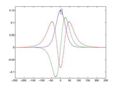
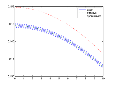
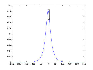
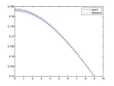
In Figures 23 and 4, below, we plot eigenfunctions of ε,αsubscript𝜀𝛼\mathcal{L}_{\varepsilon,\alpha} in the three different regimes, and compare them with the approximations involved in our results, i.e. the eigenfunction of the effective operator, ε,α𝖾𝖿𝖿superscriptsubscript𝜀𝛼𝖾𝖿𝖿\mathcal{L}_{\varepsilon,\alpha}^{\mathsf{eff}}, and its asymptotic approximation —namely φn,ε,α𝖺𝗉𝗉:=ε1+α4Hn(ε1+α2)\varphi^{\mathsf{app}}_{n,\varepsilon,\alpha}:=\varepsilon^{\frac{1+\alpha}{4}}H_{n}(\varepsilon^{\frac{1+\alpha}{2}}\cdot) in the semiclassical regime, and φε,α𝖺𝗉𝗉:=(ε2α2|V0|)12exp(||ε2α2V0)\varphi^{\mathsf{app}}_{\varepsilon,\alpha}:=\big{(}\frac{\varepsilon^{2-\alpha}}{2}\int_{\mathbb{R}}|V_{0}|\big{)}^{\frac{1}{2}}\exp\big{(}|\cdot|\frac{\varepsilon^{2-\alpha}}{2}\int_{\mathbb{R}}V_{0}\big{)} in the weak coupling regime).

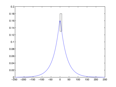
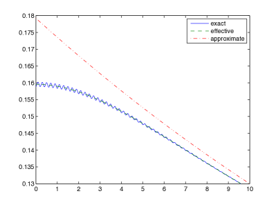
The numerical scheme used for computing the eigenfunctions is described in Appendix A. We defined the oscillatory potential by

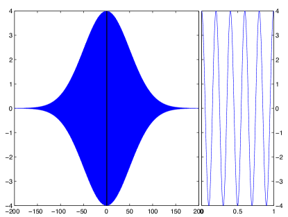
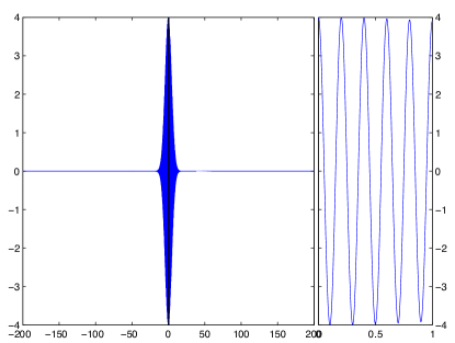
q(X,y)=4cos(2πy)×exp(X2/8),𝑞𝑋𝑦42𝜋𝑦superscript𝑋28q(X,y)=4\cos(2\pi y)\times\exp(-X^{2}/8)\,,

(see Figure 1), so that

Q(X,y)=1π2cos(2πy)×exp(X2/8),V0(X)=2π2exp(X2/4).formulae-sequence𝑄𝑋𝑦1superscript𝜋22𝜋𝑦superscript𝑋28subscript𝑉0𝑋2superscript𝜋2superscript𝑋24Q(X,y)=-\frac{1}{\pi^{2}}\cos(2\pi y)\times\exp(-X^{2}/8)\,,\qquad V_{0}(X)=-\frac{2}{\pi^{2}}\exp(-X^{2}/4)\,.

The value of the parameters are ε=1/5𝜀15\varepsilon=1/5, and α=2𝛼2\alpha=2 (semiclassical regime), α=1/2𝛼12\alpha=1/2 (weak coupling regime) and α=1𝛼1\alpha=1 (critical regime).

Refer to caption
(a) Semiclassical regime, α=2𝛼2\alpha=2, and ε=1/5𝜀15\varepsilon=1/5
Refer to caption
(b) Weak coupling regime, α=1/2𝛼12\alpha=1/2, and ε=1/5𝜀15\varepsilon=1/5
Figure 1. Large and small-scale behavior of the oscillatory potential, q(εα,/ε)q(\varepsilon^{\alpha}\cdot,\cdot/\varepsilon).
Refer to caption
(a) First three normalized eigenfunctions, ψn,ε,αsubscript𝜓𝑛𝜀𝛼\psi_{n,\varepsilon,\alpha}
Refer to caption
(b) Close-up and comparison with effective eigenfunction, φ1,ε,α𝖾𝖿𝖿subscriptsuperscript𝜑𝖾𝖿𝖿1𝜀𝛼\varphi^{\mathsf{eff}}_{1,\varepsilon,\alpha}, and its approximation, φ1,ε,α𝖺𝗉𝗉subscriptsuperscript𝜑𝖺𝗉𝗉1𝜀𝛼\varphi^{\mathsf{app}}_{1,\varepsilon,\alpha}
Figure 2. Semiclassical regime, α=2𝛼2\alpha=2.
Refer to caption
(a) Normalized eigenfunction, ψε,αsubscript𝜓𝜀𝛼\psi_{\varepsilon,\alpha}
Refer to caption
(b) Close-up and comparison with effective eigenfunction, φε,α𝖾𝖿𝖿subscriptsuperscript𝜑𝖾𝖿𝖿𝜀𝛼\varphi^{\mathsf{eff}}_{\varepsilon,\alpha}, and its approximation, φε,α𝖺𝗉𝗉subscriptsuperscript𝜑𝖺𝗉𝗉𝜀𝛼\varphi^{\mathsf{app}}_{\varepsilon,\alpha}
Figure 3. Weak coupling regime, α=1/2𝛼12\alpha=1/2.
Refer to caption
(a) First normalized eigenfunction, ψ1,εsubscript𝜓1𝜀\psi_{1,\varepsilon}
Refer to caption
(b) Close-up and comparison with effective eigenfunction, φ1,ε𝖾𝖿𝖿=εφ1,V0(ε1/2)\varphi^{\mathsf{eff}}_{1,\varepsilon}=\varepsilon\varphi_{1,V_{0}}(\varepsilon^{1/2}\cdot)
Figure 4. Critical regime, α=1𝛼1\alpha=1.

A striking observation on these numerical experiments is that, as suggested in Propositions 1.71.9 and 1.10, the main source of imprecision arises when approximating the eigenfunction of the effective problem, φ𝖾𝖿𝖿superscript𝜑𝖾𝖿𝖿\varphi^{\mathsf{eff}} with its semiclassical or weak coupling asymptotics, φ𝖺𝗉𝗉superscript𝜑𝖺𝗉𝗉\varphi^{\mathsf{app}}. Notice however that, in our results, the estimates between the exact and effective eigenfunctions is still much less precise than the eigenvalue approximation, due to the smallness of the spectral gap. As a matter of fact, the crudeness of the former estimates hides a finer structure for the eigenfunctions, suggested by our proof: we show that

ψε,α(x)eϕε(x)×φε,α𝖾𝖿𝖿(0xe2ϕε(x)dx),ϕε(x)ε2Q(εαx,x/ε).formulae-sequencesubscript𝜓𝜀𝛼𝑥superscript𝑒subscriptitalic-ϕ𝜀𝑥subscriptsuperscript𝜑𝖾𝖿𝖿𝜀𝛼superscriptsubscript0𝑥superscript𝑒2subscriptitalic-ϕ𝜀superscript𝑥differential-dsuperscript𝑥subscriptitalic-ϕ𝜀𝑥superscript𝜀2𝑄superscript𝜀𝛼𝑥𝑥𝜀\psi_{\varepsilon,\alpha}(x)\approx e^{\phi_{\varepsilon}(x)}\times\varphi^{\mathsf{eff}}_{\varepsilon,\alpha}\left(\int_{0}^{x}e^{-2\phi_{\varepsilon}(x^{\prime})}\mathrm{d}x^{\prime}\right)\,,\quad\phi_{\varepsilon}(x)\approx\varepsilon^{2}Q(\varepsilon^{\alpha}x,x/\varepsilon)\,.

Notice the above shows three different scales, as the scaling involved in φε,α𝖾𝖿𝖿subscriptsuperscript𝜑𝖾𝖿𝖿𝜀𝛼\varphi^{\mathsf{eff}}_{\varepsilon,\alpha} is different form the ones involved by ϕεsubscriptitalic-ϕ𝜀\phi_{\varepsilon}, unless α=1𝛼1\alpha=1. In particular, oscillations are localized on a smaller region than the one defined by the eigenfunction in the weak coupling regime, in contrast with the semiclassical regime (which explains why a two-scale expansion could be obtained only in this situation). Although the precision of our results is insufficient to demonstrate the refined behavior, the latter is fully supported by our numerical simulations. Indeed, had we plotted

φ~ε,α𝖾𝖿𝖿(x)=eε2Q(εαx,x/ε)×φε,α𝖾𝖿𝖿(x),subscriptsuperscript~𝜑𝖾𝖿𝖿𝜀𝛼𝑥superscript𝑒superscript𝜀2𝑄superscript𝜀𝛼𝑥𝑥𝜀subscriptsuperscript𝜑𝖾𝖿𝖿𝜀𝛼𝑥\widetilde{\varphi}^{\mathsf{eff}}_{\varepsilon,\alpha}(x)=e^{\varepsilon^{2}Q(\varepsilon^{\alpha}x,x/\varepsilon)}\times\varphi^{\mathsf{eff}}_{\varepsilon,\alpha}(x)\,,

in Figures 23 and 4, then its graph would have been superimposed with the one of the corresponding eigenfunction of the oscillatory operator, ε,αsubscript𝜀𝛼\mathcal{L}_{\varepsilon,\alpha}.

1.4. Related results and analogies in the literature

Let us now briefly discuss the relation of our results with the existing literature.

1.4.1. Homogenization

The problem of describing the large scale behavior of partial differential equations with periodically oscillating coefficients on a small scale is often tackled by the so-called homogenization process. Our approach is closely related, as the effective potential can be thought as the effective medium obtained after solving the auxiliary “cell” problem (1.4). Notice however that our problem involves three scales whereas standard works based on homogenization techniques typically involve only two scales, as in the case α=0𝛼0\alpha=0 or α=1𝛼1\alpha=1. This transpires for instance in [2, 3, 1] where, in order to deal with large potentials, the authors introduce a factorization principle which is similar to our normal form transformation (see below), although without the change of variable. We would also like to mention the recent works [22, 6, 23], where similar multiscale problem as ours are studied.

1.4.2. Effective potential

The notion of effective problems is of course ubiquitous in asymptotic studies, and in particular when a microstructure is involved. As mentioned earlier, in the specific situation α=0𝛼0\alpha=0, the effective potential V0subscript𝑉0V_{0} in (1.6) was introduced in the previous work [13]. This was then refined and generalized so as to deal with higher dimensions and scattering resonances in [11, 10]. In particular, the correction V1subscript𝑉1V_{1} in (1.6) was introduced in [11], together with the existence of a power series expansion —with the first terms being explicitly given through the effective potentials— again in the situation α=0𝛼0\alpha=0.

1.4.3. Anderson localization

It is interesting to notice that our results display a similar behavior than the one at stake in the famous Anderson localization phenomenon (see for instance [15]). In the present context, a discrete spectral structure emerges from the strong oscillations of the electric potential. Here, in some sense, the oscillations play the role of randomness. The phenomenon is weakened by the spatial decay of the potential (in particular the essential spectrum is unperturbed), however more and more discrete eigenvalues are generated as ε𝜀\varepsilon is small and α𝛼\alpha is large.

1.4.4. Born-Oppenheimer reduction

Our strategy is somewhat reminiscent of the so-called Born-Oppenheimer approximation. This method of dimensional reduction, that is a quantum averaging strategy, was initially introduced in [5] (see also [19] in relation with molecular physics) and has been developed in many different contexts (see for instance the review [17]), and in particular to derive spectral asymptotic results (see [20, 25]). Let us explain the analogy. Consider the two-dimensional operator

Dx12+Dx22+q(εαx1,ε1x2),subscriptsuperscript𝐷2subscript𝑥1subscriptsuperscript𝐷2subscript𝑥2𝑞superscript𝜀𝛼subscript𝑥1superscript𝜀1subscript𝑥2D^{2}_{x_{1}}+D^{2}_{x_{2}}+q(\varepsilon^{\alpha}x_{1},\varepsilon^{-1}x_{2})\,,

acting on L2(×𝕋)superscript𝐿2𝕋L^{2}(\mathbb{R}\times{\mathbb{T}}) with q𝑞q satisfying the same assumptions as above. This operator is formally obtained by introducing a fictitious variable x2subscript𝑥2x_{2} and duplicating the second derivative. Using the rescaling y=ε1x2𝑦superscript𝜀1subscript𝑥2y=\varepsilon^{-1}x_{2}, we are reduced to the unitarily equivalent operator:

Dx12+ε2Dy2+q(εαx1,y).subscriptsuperscript𝐷2subscript𝑥1superscript𝜀2subscriptsuperscript𝐷2𝑦𝑞superscript𝜀𝛼subscript𝑥1𝑦D^{2}_{x_{1}}+\varepsilon^{-2}D^{2}_{y}+q(\varepsilon^{\alpha}x_{1},y)\,.

This operator is in the Born-Oppenheimer form: it is partially semiclassical with respect to the variable x1subscript𝑥1x_{1} and εαx1,ε=ε2Dy2+q(εαx1,y)subscriptsuperscript𝜀𝛼subscript𝑥1𝜀superscript𝜀2subscriptsuperscript𝐷2𝑦𝑞superscript𝜀𝛼subscript𝑥1𝑦\mathcal{M}_{\varepsilon^{\alpha}x_{1},\varepsilon}=\varepsilon^{-2}D^{2}_{y}+q(\varepsilon^{\alpha}x_{1},y) can be interpreted as an operator-valued potential. It can be proved in a rather general framework (see for instance [21] in the context of pseudo-differential operators) that, generically, the low-lying spectrum is well described by the one of the reduced operator

Dx12+με(εαx1)Dx12+ε2V0(εαx1).subscriptsuperscript𝐷2subscript𝑥1subscript𝜇𝜀superscript𝜀𝛼subscript𝑥1subscriptsuperscript𝐷2subscript𝑥1superscript𝜀2subscript𝑉0superscript𝜀𝛼subscript𝑥1D^{2}_{x_{1}}+\mu_{\varepsilon}(\varepsilon^{\alpha}x_{1})\approx D^{2}_{x_{1}}+\varepsilon^{2}V_{0}(\varepsilon^{\alpha}x_{1})\,.

The study here is complicated by the presence of cross-derivatives Dx1Dx2subscript𝐷subscript𝑥1subscript𝐷subscript𝑥2D_{x_{1}}D_{x_{2}}, due to the fact that the variables x1subscript𝑥1x_{1} and x2subscript𝑥2x_{2} are not independent. The above strategy however served as a guideline for the construction of the normal form in a previous version of this work [12].

1.4.5. Weakly decaying oscillating potentials

The strategy of our paper follows some ideas of [24], where the author studies the asymptotic distribution of discrete eigenvalues of the Schrödinger operator with weakly decaying (non-rapidly) oscillating potentials. It is well-known that if the potential is negative at infinity, then the asymptotic distribution of discrete eigenvalues is driven by the decay rate of the potential [26], but no results were known when the potential oscillates at infinity. Here again, the effective potential plays a role as it allows to predict the correct behavior of the asymptotic distribution of discrete eigenvalues.

1.5. Strategy and outline

Let us describe the key elements of the proof of our results. The main idea is a normal form transformation. We show that the contributions of the oscillatory potential q(εαx,x/ε)𝑞superscript𝜀𝛼𝑥𝑥𝜀q(\varepsilon^{\alpha}x,x/\varepsilon) may be approximately factorized thanks to a two-scale function ϕε(x)=ε2Φε(εαx,x/ε)subscriptitalic-ϕ𝜀𝑥superscript𝜀2subscriptΦ𝜀superscript𝜀𝛼𝑥𝑥𝜀\phi_{\varepsilon}(x)=\varepsilon^{2}\Phi_{\varepsilon}(\varepsilon^{\alpha}x,x/\varepsilon). This function plays the role of a complex phase, and is chosen after considering the operator eϕεε,αeϕεsuperscript𝑒subscriptitalic-ϕ𝜀subscript𝜀𝛼superscript𝑒subscriptitalic-ϕ𝜀e^{-\phi_{\varepsilon}}\mathcal{L}_{\varepsilon,\alpha}e^{\phi_{\varepsilon}} and so that

q(εαx,x/ε)ϕε,α′′(x)(ϕε,α)2(x)=Vε(εαx)+rε(x),𝑞superscript𝜀𝛼𝑥𝑥𝜀superscriptsubscriptitalic-ϕ𝜀𝛼′′𝑥superscriptsuperscriptsubscriptitalic-ϕ𝜀𝛼2𝑥subscript𝑉𝜀superscript𝜀𝛼𝑥subscript𝑟𝜀𝑥q(\varepsilon^{\alpha}x,x/\varepsilon)-\phi_{\varepsilon,\alpha}^{\prime\prime}(x)-(\phi_{\varepsilon,\alpha}^{\prime})^{2}(x)=V_{\varepsilon}(\varepsilon^{\alpha}x)+r_{\varepsilon}(x),

where Vεsubscript𝑉𝜀V_{\varepsilon} depends only on the large scale and rεsubscript𝑟𝜀r_{\varepsilon} is a small remainder. We explain in Section 2.1 how ϕεsubscriptitalic-ϕ𝜀\phi_{\varepsilon} may be explicitly constructed and how the effective potential Vε=ε2V0+ε3+αV1subscript𝑉𝜀superscript𝜀2subscript𝑉0superscript𝜀3𝛼subscript𝑉1V_{\varepsilon}=\varepsilon^{2}V_{0}+\varepsilon^{3+\alpha}V_{1} emerges from this construction. The normal form of the operator is made explicit and compared with the effective operator, ε,α𝖾𝖿𝖿superscriptsubscript𝜀𝛼𝖾𝖿𝖿\mathcal{L}_{\varepsilon,\alpha}^{\mathsf{eff}}, in Section 2.2.

In Section 3, we apply the normal form transformation so as to compare the Rayleigh quotients associated with ε,αsubscript𝜀𝛼\mathcal{L}_{\varepsilon,\alpha} and the ones associated with ε,α𝖾𝖿𝖿superscriptsubscript𝜀𝛼𝖾𝖿𝖿\mathcal{L}_{\varepsilon,\alpha}^{\mathsf{eff}}. Theorem 1.4 quickly follows from the min-max principle. We then deduce the asymptotic behavior of the eigenvalues in the three aforementioned regimes.

In Section 4, we use again the normal form of our operator to construct quasimodes. We detail in Section 4.1 (respectively Section 4.2 and Section 4.3) the semiclassical regime, α>1𝛼1\alpha>1 (respectively weak coupling regime, α<1𝛼1\alpha<1 and critical regime, α=1𝛼1\alpha=1). By using the classical resolvent bound for self-adjoint operators (consequence of the spectral theorem), together with the previously obtained results on the eigenvalues, allows to deduce the asymptotic behavior of the corresponding eigenfunctions, as stated above.

Section 5 is devoted to the case α=2𝛼2\alpha=2 and to the proof of the two-scale WKB expansion stated in Proposition 1.11.

2. The normal form

As mentioned earlier, the key ingredient of our analysis is a “normal form” of our operator, obtained through conjugation. The conjugation allows to replace the main oscillatory contributions by a large-scale, effective potential. More precisely, we shall introduce the transformation

𝖳ϕε:φψ,ψ(x):=eϕε,α(x)φ(0xe2ϕε,α(x)dx),:subscript𝖳subscriptitalic-ϕ𝜀formulae-sequencemaps-to𝜑𝜓assign𝜓𝑥superscript𝑒subscriptitalic-ϕ𝜀𝛼𝑥𝜑superscriptsubscript0𝑥superscript𝑒2subscriptitalic-ϕ𝜀𝛼superscript𝑥differential-dsuperscript𝑥{\sf T}_{\phi_{\varepsilon}}:\varphi\mapsto\psi,\quad\psi(x):=e^{\phi_{\varepsilon,\alpha}(x)}\varphi\left(\int_{0}^{x}e^{-2\phi_{\varepsilon,\alpha}(x^{\prime})}\mathrm{d}x^{\prime}\right),

where ϕε,αsubscriptitalic-ϕ𝜀𝛼\phi_{\varepsilon,\alpha} is to be determined. This yields a new Schrödinger operator involving the reduced potential (up to a complex phase which will not play a role in our analysis)

Vϕε,α(x):=q(εαx,x/ε)ϕε,α′′(x)(ϕε,α)2(x).assignsubscript𝑉subscriptitalic-ϕ𝜀𝛼𝑥𝑞superscript𝜀𝛼𝑥𝑥𝜀superscriptsubscriptitalic-ϕ𝜀𝛼′′𝑥superscriptsuperscriptsubscriptitalic-ϕ𝜀𝛼2𝑥V_{\phi_{\varepsilon,\alpha}}(x):=q(\varepsilon^{\alpha}x,x/\varepsilon)-\phi_{\varepsilon,\alpha}^{\prime\prime}(x)-(\phi_{\varepsilon,\alpha}^{\prime})^{2}(x).

Our aim is to choose ϕε,αsubscriptitalic-ϕ𝜀𝛼\phi_{\varepsilon,\alpha} such that Vϕε,αsubscript𝑉subscriptitalic-ϕ𝜀𝛼V_{\phi_{\varepsilon,\alpha}} depends only on the large-scale variable (up to a small oscillatory term). We explain in section 2.1 how we obtain such a phase and how the effective potential surfaces. We then apply these results to our Schrödinger operator, and provide useful estimates in Section 2.2

2.1. Construction of the phase

Our aim in this section is to exhibit a complex phase, ϕε,α(x)subscriptitalic-ϕ𝜀𝛼𝑥\phi_{\varepsilon,\alpha}(x), such that

(2.1) q(εαx,x/ε)ϕε,α′′(x)(ϕε,α)2(x)=Vε(εαx)+rε,𝑞superscript𝜀𝛼𝑥𝑥𝜀superscriptsubscriptitalic-ϕ𝜀𝛼′′𝑥superscriptsuperscriptsubscriptitalic-ϕ𝜀𝛼2𝑥subscript𝑉𝜀superscript𝜀𝛼𝑥subscript𝑟𝜀q(\varepsilon^{\alpha}x,x/\varepsilon)-\phi_{\varepsilon,\alpha}^{\prime\prime}(x)-(\phi_{\varepsilon,\alpha}^{\prime})^{2}(x)=V_{\varepsilon}(\varepsilon^{\alpha}x)+r_{\varepsilon},

where the remainder term rεsubscript𝑟𝜀r_{\varepsilon} is as small as desired. We seek ϕε,αsubscriptitalic-ϕ𝜀𝛼\phi_{\varepsilon,\alpha} (and consequently rεsubscript𝑟𝜀r_{\varepsilon}) with two-scale behavior

ϕε,α(x)=ε2Φε(εαx,x/ε),subscriptitalic-ϕ𝜀𝛼𝑥superscript𝜀2subscriptΦ𝜀superscript𝜀𝛼𝑥𝑥𝜀\phi_{\varepsilon,\alpha}(x)=\varepsilon^{2}\Phi_{\varepsilon}(\varepsilon^{\alpha}x,x/\varepsilon),

where the profile ΦεsubscriptΦ𝜀\Phi_{\varepsilon} has to be determined. Equation (2.1) becomes

(Dy2+2ε1+αDXDy+ε2(1+α)DX2)Φε(X,y)+ε2(DyΦε+ε1+αDXΦε)2(X,y)+q(X,y)=Vε(X)+rε(X,y).superscriptsubscript𝐷𝑦22superscript𝜀1𝛼subscript𝐷𝑋subscript𝐷𝑦superscript𝜀21𝛼superscriptsubscript𝐷𝑋2subscriptΦ𝜀𝑋𝑦superscript𝜀2superscriptsubscript𝐷𝑦subscriptΦ𝜀superscript𝜀1𝛼subscript𝐷𝑋subscriptΦ𝜀2𝑋𝑦𝑞𝑋𝑦subscript𝑉𝜀𝑋subscript𝑟𝜀𝑋𝑦\left(D_{y}^{2}+2\varepsilon^{1+\alpha}D_{X}D_{y}+\varepsilon^{2(1+\alpha)}D_{X}^{2}\right)\Phi_{\varepsilon}(X,y)\\ +\varepsilon^{2}\left(D_{y}\Phi_{\varepsilon}+\varepsilon^{1+\alpha}D_{X}\Phi_{\varepsilon}\right)^{2}(X,y)+q(X,y)=V_{\varepsilon}(X)+r_{\varepsilon}(X,y).

Consistently, we will solve the above with the following Ansatz:

Φε(X,y)=κ2εp(κ)Φκ(X,y),Vε(X)=κ2εp(κ)Φκ(X,y)formulae-sequencesubscriptΦ𝜀𝑋𝑦subscript𝜅superscript2superscript𝜀𝑝𝜅subscriptΦ𝜅𝑋𝑦subscript𝑉𝜀𝑋subscript𝜅superscript2superscript𝜀𝑝𝜅subscriptΦ𝜅𝑋𝑦\Phi_{\varepsilon}(X,y)=\sum_{\kappa\in\mathbb{N}^{2}}\varepsilon^{p(\kappa)}\Phi_{\kappa}(X,y),\quad V_{\varepsilon}(X)=\sum_{\kappa\in\mathbb{N}^{2}}\varepsilon^{p(\kappa)}\Phi_{\kappa}(X,y)

where p(κ1,κ2):=(1+α)κ1+2κ2assign𝑝subscript𝜅1subscript𝜅21𝛼subscript𝜅12subscript𝜅2p(\kappa_{1},\kappa_{2}):=(1+\alpha)\kappa_{1}+2\kappa_{2}, and we additionally enforce the property

κ2,𝕋Φκ(X,y)dy=0.formulae-sequencefor-all𝜅superscript2subscript𝕋subscriptΦ𝜅𝑋𝑦differential-d𝑦0\forall\kappa\in\mathbb{N}^{2},\quad\int_{\mathbb{T}}\Phi_{\kappa}(X,y)\mathrm{d}y=0.

2.1.1. Inductive construction

Plugging the Ansatz into the equation and solving at order (κ1,κ2)subscript𝜅1subscript𝜅2(\kappa_{1},\kappa_{2}) yields

Dy2Φκ1,κ2+2DXDyΦκ11,κ2+DX2Φκ12,κ2+κ3=0κ1(DyΦκ3,κ21)(DyΦκ1κ3,κ21)+κ3=1κ1(DyΦκ31,κ21)(DXΦκ1κ3,κ21)+κ3=2κ1(DXΦκ32,κ21)(DXΦκ1κ3,κ21)=δ(κ1,κ2)=(0,0)q+Vκ1,κ2,superscriptsubscript𝐷𝑦2subscriptΦsubscript𝜅1subscript𝜅22subscript𝐷𝑋subscript𝐷𝑦subscriptΦsubscript𝜅11subscript𝜅2superscriptsubscript𝐷𝑋2subscriptΦsubscript𝜅12subscript𝜅2superscriptsubscriptsubscript𝜅30subscript𝜅1subscript𝐷𝑦subscriptΦsubscript𝜅3subscript𝜅21subscript𝐷𝑦subscriptΦsubscript𝜅1subscript𝜅3subscript𝜅21superscriptsubscriptsubscript𝜅31subscript𝜅1subscript𝐷𝑦subscriptΦsubscript𝜅31subscript𝜅21subscript𝐷𝑋subscriptΦsubscript𝜅1subscript𝜅3subscript𝜅21superscriptsubscriptsubscript𝜅32subscript𝜅1subscript𝐷𝑋subscriptΦsubscript𝜅32subscript𝜅21subscript𝐷𝑋subscriptΦsubscript𝜅1subscript𝜅3subscript𝜅21subscript𝛿subscript𝜅1subscript𝜅200𝑞subscript𝑉subscript𝜅1subscript𝜅2D_{y}^{2}\Phi_{\kappa_{1},\kappa_{2}}+2D_{X}D_{y}\Phi_{\kappa_{1}-1,\kappa_{2}}+D_{X}^{2}\Phi_{\kappa_{1}-2,\kappa_{2}}\\ +\sum_{\kappa_{3}=0}^{\kappa_{1}}(D_{y}\Phi_{\kappa_{3},\kappa_{2}-1})(D_{y}\Phi_{\kappa_{1}-\kappa_{3},\kappa_{2}-1})+\sum_{\kappa_{3}=1}^{\kappa_{1}}(D_{y}\Phi_{\kappa_{3}-1,\kappa_{2}-1})(D_{X}\Phi_{\kappa_{1}-\kappa_{3},\kappa_{2}-1})\\ +\sum_{\kappa_{3}=2}^{\kappa_{1}}(D_{X}\Phi_{\kappa_{3}-2,\kappa_{2}-1})(D_{X}\Phi_{\kappa_{1}-\kappa_{3},\kappa_{2}-1})=-\delta_{(\kappa_{1},\kappa_{2})=(0,0)}q+V_{\kappa_{1},\kappa_{2}},

where δ(κ1,κ2)=(0,0)=1subscript𝛿subscript𝜅1subscript𝜅2001\delta_{(\kappa_{1},\kappa_{2})=(0,0)}=1 if (κ1,κ2)=(0,0)subscript𝜅1subscript𝜅200(\kappa_{1},\kappa_{2})=(0,0) and 00 otherwise.

We may define Φκ1,κ2subscriptΦsubscript𝜅1subscript𝜅2\Phi_{\kappa_{1},\kappa_{2}} and Vκ1,κ2subscript𝑉subscript𝜅1subscript𝜅2V_{\kappa_{1},\kappa_{2}} by induction on |κ|=κ1+κ2𝜅subscript𝜅1subscript𝜅2|\kappa|=\kappa_{1}+\kappa_{2}. Indeed, the equation reads

Dy2Φκ1,κ2(X,y)+Fκ1,κ2(X,y)=Vκ1,κ2(X),superscriptsubscript𝐷𝑦2subscriptΦsubscript𝜅1subscript𝜅2𝑋𝑦subscript𝐹subscript𝜅1subscript𝜅2𝑋𝑦subscript𝑉subscript𝜅1subscript𝜅2𝑋D_{y}^{2}\Phi_{\kappa_{1},\kappa_{2}}(X,y)+F_{\kappa_{1},\kappa_{2}}(X,y)=V_{\kappa_{1},\kappa_{2}}(X),

where Fκ1,κ2(X,y)subscript𝐹subscript𝜅1subscript𝜅2𝑋𝑦F_{\kappa_{1},\kappa_{2}}(X,y) is given explicitly in terms of ΦκsubscriptΦsuperscript𝜅\Phi_{\kappa^{\prime}} with |κ||κ1|superscript𝜅𝜅1|\kappa^{\prime}|\leq|\kappa-1|. We solve the equation by setting (as forced by the Fredholm alternative in the variable y𝑦y)

Vκ1,κ2(X)=𝕋Fκ1,κ2(X,y)dy,subscript𝑉subscript𝜅1subscript𝜅2𝑋subscript𝕋subscript𝐹subscript𝜅1subscript𝜅2𝑋𝑦differential-d𝑦V_{\kappa_{1},\kappa_{2}}(X)=\int_{\mathbb{T}}F_{\kappa_{1},\kappa_{2}}(X,y)\mathrm{d}y,

and then Φκ1,κ2subscriptΦsubscript𝜅1subscript𝜅2\Phi_{\kappa_{1},\kappa_{2}} is the unique mean-zero solution to

Dy2Φκ1,κ2(X,y)=Vκ1,κ2(X)Fκ1,κ2(X,y).superscriptsubscript𝐷𝑦2subscriptΦsubscript𝜅1subscript𝜅2𝑋𝑦subscript𝑉subscript𝜅1subscript𝜅2𝑋subscript𝐹subscript𝜅1subscript𝜅2𝑋𝑦D_{y}^{2}\Phi_{\kappa_{1},\kappa_{2}}(X,y)=V_{\kappa_{1},\kappa_{2}}(X)-F_{\kappa_{1},\kappa_{2}}(X,y).

Let us detail the first terms. At order κ=(0,0)𝜅00\kappa=(0,0), one finds

Dy2Φ0,0(X,y)+q(X,y)=V0,0(X).superscriptsubscript𝐷𝑦2subscriptΦ00𝑋𝑦𝑞𝑋𝑦subscript𝑉00𝑋D_{y}^{2}\Phi_{0,0}(X,y)+q(X,y)=V_{0,0}(X).

Because , yq(X,y)maps-to𝑦𝑞𝑋𝑦y\mapsto q(X,y) is mean-zero, we deduce

V0,0(X)=0 and Φ0,0(X,y)=Q(X,y),formulae-sequencesubscript𝑉00𝑋0 and subscriptΦ00𝑋𝑦𝑄𝑋𝑦V_{0,0}(X)=0\quad\text{ and }\quad\Phi_{0,0}(X,y)=Q(X,y),

where we recall that Q(X,)𝑄𝑋Q(X,\cdot) is the zero-mean solution to Dy2Q(X,y)=q(X,y)superscriptsubscript𝐷𝑦2𝑄𝑋𝑦𝑞𝑋𝑦D_{y}^{2}Q(X,y)=-q(X,y). At order κ=(1,0)𝜅10\kappa=(1,0), one has

Dy2Φ1,0(X,y)+2DXDyΦ0,0(X,y)=V1,0(X).superscriptsubscript𝐷𝑦2subscriptΦ10𝑋𝑦2subscript𝐷𝑋subscript𝐷𝑦subscriptΦ00𝑋𝑦subscript𝑉10𝑋D_{y}^{2}\Phi_{1,0}(X,y)+2D_{X}D_{y}\Phi_{0,0}(X,y)=V_{1,0}(X).

We deduce

V1,0(X)=0 and Dy2Φ1,0(X,y)=2DXDyQ(X,y).formulae-sequencesubscript𝑉10𝑋0 and superscriptsubscript𝐷𝑦2subscriptΦ10𝑋𝑦2subscript𝐷𝑋subscript𝐷𝑦𝑄𝑋𝑦V_{1,0}(X)=0\quad\text{ and }\quad D_{y}^{2}\Phi_{1,0}(X,y)=-2D_{X}D_{y}Q(X,y).

At order (k,0)𝑘0(k,0), for k2𝑘2k\geq 2, one has

Dy2Φk,0(X,y)+2DXDyΦk1,0(X,y)+DX2Φk2,0(X,y)=Vk,0(X).superscriptsubscript𝐷𝑦2subscriptΦ𝑘0𝑋𝑦2subscript𝐷𝑋subscript𝐷𝑦subscriptΦ𝑘10𝑋𝑦superscriptsubscript𝐷𝑋2subscriptΦ𝑘20𝑋𝑦subscript𝑉𝑘0𝑋D_{y}^{2}\Phi_{k,0}(X,y)+2D_{X}D_{y}\Phi_{k-1,0}(X,y)+D_{X}^{2}\Phi_{k-2,0}(X,y)=V_{k,0}(X).

We deduce

Vk,0(X)=0 and Dy2Φk,0=2DXDyΦk1,0DX2Φk2,0.formulae-sequencesubscript𝑉𝑘0𝑋0 and superscriptsubscript𝐷𝑦2subscriptΦ𝑘02subscript𝐷𝑋subscript𝐷𝑦subscriptΦ𝑘10superscriptsubscript𝐷𝑋2subscriptΦ𝑘20V_{k,0}(X)=0\quad\text{ and }\quad D_{y}^{2}\Phi_{k,0}=-2D_{X}D_{y}\Phi_{k-1,0}-D_{X}^{2}\Phi_{k-2,0}.

In particular,

Dy2Φ2,0=3DX2Q and Dy2Φ2,0=2DX2Φ1,0.formulae-sequencesuperscriptsubscript𝐷𝑦2subscriptΦ203superscriptsubscript𝐷𝑋2𝑄 and superscriptsubscript𝐷𝑦2subscriptΦ202superscriptsubscript𝐷𝑋2subscriptΦ10D_{y}^{2}\Phi_{2,0}=3D_{X}^{2}Q\quad\text{ and }\quad D_{y}^{2}\Phi_{2,0}=2D_{X}^{2}\Phi_{1,0}.

At order κ=(0,1)𝜅01\kappa=(0,1), we find

Dy2Φ0,1(X,y)+(DyΦ0,0)2(X,y)=V0,1(X).superscriptsubscript𝐷𝑦2subscriptΦ01𝑋𝑦superscriptsubscript𝐷𝑦subscriptΦ002𝑋𝑦subscript𝑉01𝑋D_{y}^{2}\Phi_{0,1}(X,y)+(D_{y}\Phi_{0,0})^{2}(X,y)=V_{0,1}(X).

We deduce from the Fredholm alternative

V0,1(X)=𝕋(DyQ)2dy=:V0(X),V_{0,1}(X)=\int_{\mathbb{T}}(D_{y}Q)^{2}\mathrm{d}y=:V_{0}(X),

where V0subscript𝑉0V_{0} was already defined in (1.5), and

Dy2Φ0,1=(DyQ)2(X,y)V0(X).superscriptsubscript𝐷𝑦2subscriptΦ01superscriptsubscript𝐷𝑦𝑄2𝑋𝑦subscript𝑉0𝑋D_{y}^{2}\Phi_{0,1}=-(D_{y}Q)^{2}(X,y)-V_{0}(X).

At order κ=(1,1)𝜅11\kappa=(1,1), one has

Dy2Φ1,1+2(DyΦ1,0)(DyΦ0,0)+2(DXΦ0,0)(DyΦ0,0)+2DXDyΦ0,1=V1,1.superscriptsubscript𝐷𝑦2subscriptΦ112subscript𝐷𝑦subscriptΦ10subscript𝐷𝑦subscriptΦ002subscript𝐷𝑋subscriptΦ00subscript𝐷𝑦subscriptΦ002subscript𝐷𝑋subscript𝐷𝑦subscriptΦ01subscript𝑉11D_{y}^{2}\Phi_{1,1}+2(D_{y}\Phi_{1,0})(D_{y}\Phi_{0,0})+2(D_{X}\Phi_{0,0})(D_{y}\Phi_{0,0})+2D_{X}D_{y}\Phi_{0,1}=V_{1,1}.

This yields, as above,

V1,1(X)=2𝕋((DyQ)(DXQ))(X,y)dy=:V1(X).V_{1,1}(X)=-2\int_{\mathbb{T}}\big{(}(D_{y}Q)(D_{X}Q)\big{)}(X,y)\mathrm{d}y=:V_{1}(X).

where V1subscript𝑉1V_{1} was also defined in (1.5), and

Dy2Φ1,1(X,y)=V1,1(X)+2((DyQ)(DXQ))(X,y)2DXDy((DyQ)2)(X,y).superscriptsubscript𝐷𝑦2subscriptΦ11𝑋𝑦subscript𝑉11𝑋2subscript𝐷𝑦𝑄subscript𝐷𝑋𝑄𝑋𝑦2subscript𝐷𝑋subscript𝐷𝑦superscriptsubscript𝐷𝑦𝑄2𝑋𝑦D_{y}^{2}\Phi_{1,1}(X,y)=V_{1,1}(X)+2\big{(}(D_{y}Q)(D_{X}Q)\big{)}(X,y)-2D_{X}D_{y}\big{(}(D_{y}Q)^{2}\big{)}(X,y).

2.1.2. Truncated expansion

As it is clear from the previous section, we can solve the problem up to any arbitrary high order provided that qW,(×𝕋)𝑞subscriptsuperscript𝑊𝕋{q\in\bigcap_{\ell\in\mathbb{N}}W^{\ell,\infty}(\mathbb{R}\times{\mathbb{T}})}. Unfortunately, other sources of error cannot be avoided, and our results do not benefit from adding all high-order contributions in the expansion. Here we decide to truncate the expansion so as to satisfy (2.1) with precision 𝒪(εmin{4,2+2(1+α),4(1+α)})𝒪superscript𝜀4221𝛼41𝛼\mathcal{O}(\varepsilon^{\min\{4,2+2(1+\alpha),4(1+\alpha)\}}).

Definition 2.1.

For ε>0𝜀0\varepsilon>0 and qW3,(×𝕋)𝑞superscript𝑊3𝕋q\in W^{3,\infty}(\mathbb{R}\times{\mathbb{T}}), we set

ϕε,α(x)=ε2(k=03εk(1+α)Φk,0+ε2Φ0,1+ε3+αΦ1,1)(εαx,x/ε),subscriptitalic-ϕ𝜀𝛼𝑥superscript𝜀2superscriptsubscript𝑘03superscript𝜀𝑘1𝛼subscriptΦ𝑘0superscript𝜀2subscriptΦ01superscript𝜀3𝛼subscriptΦ11superscript𝜀𝛼𝑥𝑥𝜀\phi_{\varepsilon,\alpha}(x)=\varepsilon^{2}\left(\sum_{k=0}^{3}\varepsilon^{k(1+\alpha)}\Phi_{k,0}+\varepsilon^{2}\Phi_{0,1}+\varepsilon^{3+\alpha}\Phi_{1,1}\right)(\varepsilon^{\alpha}x,x/\varepsilon),

where Φκ1,κ2subscriptΦsubscript𝜅1subscript𝜅2\Phi_{\kappa_{1},\kappa_{2}} are defined as the unique mean-zero solutions to

Dy2Φ0,0=q,Dy2Φ1,0=2DXDyΦ0,0Dy2Φ2,0=3DX2Φ0,0,formulae-sequencesuperscriptsubscript𝐷𝑦2subscriptΦ00𝑞formulae-sequencesuperscriptsubscript𝐷𝑦2subscriptΦ102subscript𝐷𝑋subscript𝐷𝑦subscriptΦ00superscriptsubscript𝐷𝑦2subscriptΦ203superscriptsubscript𝐷𝑋2subscriptΦ00\displaystyle-D_{y}^{2}\Phi_{0,0}=q,\qquad-D_{y}^{2}\Phi_{1,0}=2D_{X}D_{y}\Phi_{0,0}\,\qquad-D_{y}^{2}\Phi_{2,0}=-3D_{X}^{2}\Phi_{0,0},
Dy2Φ3,0=2DX2Φ1,0,Dy2Φ0,1=(DyΦ0,0)2𝕋(DyΦ0,0)2dy,formulae-sequencesuperscriptsubscript𝐷𝑦2subscriptΦ302superscriptsubscript𝐷𝑋2subscriptΦ10superscriptsubscript𝐷𝑦2subscriptΦ01superscriptsubscript𝐷𝑦subscriptΦ002subscript𝕋superscriptsubscript𝐷𝑦subscriptΦ002differential-d𝑦\displaystyle-D_{y}^{2}\Phi_{3,0}=-2D_{X}^{2}\Phi_{1,0},\qquad-D_{y}^{2}\Phi_{0,1}=(D_{y}\Phi_{0,0})^{2}-\int_{\mathbb{T}}(D_{y}\Phi_{0,0})^{2}\mathrm{d}y,
Dy2Φ0,1=2(DyΦ0,0)(DXΦ0,0)+2𝕋(DyΦ0,0)(DXΦ0,0)dy+2DXDyΦ0,1.superscriptsubscript𝐷𝑦2subscriptΦ012subscript𝐷𝑦subscriptΦ00subscript𝐷𝑋subscriptΦ002subscript𝕋subscript𝐷𝑦subscriptΦ00subscript𝐷𝑋subscriptΦ00differential-d𝑦2subscript𝐷𝑋subscript𝐷𝑦subscriptΦ01\displaystyle-D_{y}^{2}\Phi_{0,1}=-2(D_{y}\Phi_{0,0})(D_{X}\Phi_{0,0})+2\int_{\mathbb{T}}(D_{y}\Phi_{0,0})(D_{X}\Phi_{0,0})\mathrm{d}y+2D_{X}D_{y}\Phi_{0,1}.
Lemma 2.2.

Assume α>1𝛼1\alpha>-1 and qW5,(×𝕋)𝑞superscript𝑊5𝕋q\in W^{5,\infty}(\mathbb{R}\times{\mathbb{T}}). Then one has

eϕε,αW2,()+eϕε,αW2,()C(qW3,(×𝕋)),subscriptdelimited-∥∥superscript𝑒subscriptitalic-ϕ𝜀𝛼superscript𝑊2subscriptdelimited-∥∥superscript𝑒subscriptitalic-ϕ𝜀𝛼superscript𝑊2𝐶subscriptdelimited-∥∥𝑞superscript𝑊3𝕋\big{\lVert}e^{-\phi_{\varepsilon,\alpha}}\big{\rVert}_{W^{2,\infty}(\mathbb{R})}+\big{\lVert}e^{\phi_{\varepsilon,\alpha}}\big{\rVert}_{W^{2,\infty}(\mathbb{R})}\leq C(\big{\lVert}q\big{\rVert}_{W^{3,\infty}(\mathbb{R}\times{\mathbb{T}})})\,,
eϕε,α1L()ε2C(qW3,(×𝕋)),subscriptdelimited-∥∥superscript𝑒subscriptitalic-ϕ𝜀𝛼1superscript𝐿superscript𝜀2𝐶subscriptdelimited-∥∥𝑞superscript𝑊3𝕋\big{\lVert}e^{\phi_{\varepsilon,\alpha}}-1\big{\rVert}_{L^{\infty}(\mathbb{R})}\leq\varepsilon^{2}C(\big{\lVert}q\big{\rVert}_{W^{3,\infty}(\mathbb{R}\times{\mathbb{T}})})\,,

and

q(εα,/ε)ϕε,α′′(ϕε,α)2Vε(εα)L()εmin{4,4(1+α)}C(qW5,(×𝕋)),\big{\lVert}q(\varepsilon^{\alpha}\cdot,\cdot/\varepsilon)-\phi_{\varepsilon,\alpha}^{\prime\prime}-(\phi_{\varepsilon,\alpha}^{\prime})^{2}-V_{\varepsilon}(\varepsilon^{\alpha}\cdot)\big{\rVert}_{L^{\infty}(\mathbb{R})}\leq\varepsilon^{\min\{4,4(1+\alpha)\}}C(\big{\lVert}q\big{\rVert}_{W^{5,\infty}(\mathbb{R}\times{\mathbb{T}})})\,,

where we define

Vε(X)subscript𝑉𝜀𝑋\displaystyle V_{\varepsilon}(X) =ε2𝕋|yQ|2(X,y)dy+ 2ε3+α𝕋((xQ)(yQ))(X,y)dyabsentsuperscript𝜀2subscript𝕋superscriptsubscript𝑦𝑄2𝑋𝑦differential-d𝑦2superscript𝜀3𝛼subscript𝕋subscript𝑥𝑄subscript𝑦𝑄𝑋𝑦differential-d𝑦\displaystyle=-\varepsilon^{2}\int_{\mathbb{T}}\lvert\partial_{y}Q\rvert^{2}(X,y)\mathrm{d}y\ +\ 2\varepsilon^{3+\alpha}\int_{\mathbb{T}}\big{(}(\partial_{x}Q)(\partial_{y}Q)\big{)}(X,y)\mathrm{d}y
=:ε2V0(X)+ε3+αV1(X).\displaystyle=:\varepsilon^{2}V_{0}(X)+\varepsilon^{3+\alpha}V_{1}(X)\,.

Here, Q𝑄Q is defined by (1.4) and satisfies

QW1,(×𝕋)+DyQL(×𝕋)C(qW1,(×𝕋)).subscriptdelimited-∥∥𝑄superscript𝑊1𝕋subscriptdelimited-∥∥subscript𝐷𝑦𝑄superscript𝐿𝕋𝐶subscriptdelimited-∥∥𝑞superscript𝑊1𝕋\big{\lVert}Q\big{\rVert}_{W^{1,\infty}(\mathbb{R}\times{\mathbb{T}})}+\big{\lVert}D_{y}Q\big{\rVert}_{L^{\infty}(\mathbb{R}\times{\mathbb{T}})}\leq C(\big{\lVert}q\big{\rVert}_{W^{1,\infty}(\mathbb{R}\times{\mathbb{T}})}).
Proof.

Let us start with the last estimate of the statement. We test (1.4) with Q𝑄Q, integrate by parts and use Cauchy-Schwarz inequality to deduce

DyQ(X,)L2(𝕋)2qL(×𝕋)Q(X,)L2(𝕋)12πqL(×𝕋)DyQ(X,)L2(𝕋),subscriptsuperscriptdelimited-∥∥subscript𝐷𝑦𝑄𝑋2superscript𝐿2𝕋subscriptdelimited-∥∥𝑞superscript𝐿𝕋subscriptdelimited-∥∥𝑄𝑋superscript𝐿2𝕋12𝜋subscriptdelimited-∥∥𝑞superscript𝐿𝕋subscriptdelimited-∥∥subscript𝐷𝑦𝑄𝑋superscript𝐿2𝕋\big{\lVert}D_{y}Q(X,\cdot)\big{\rVert}^{2}_{L^{2}({\mathbb{T}})}\leq\big{\lVert}q\big{\rVert}_{L^{\infty}(\mathbb{R}\times{\mathbb{T}})}\big{\lVert}Q(X,\cdot)\big{\rVert}_{L^{2}({\mathbb{T}})}\leq\frac{1}{2\pi}\big{\lVert}q\big{\rVert}_{L^{\infty}(\mathbb{R}\times{\mathbb{T}})}\big{\lVert}D_{y}Q(X,\cdot)\big{\rVert}_{L^{2}({\mathbb{T}})}\,,

where we used Wirtinger’s inequality (or the min-max principle since the mean value of Q𝑄Q is zero, and the second lowest eigenvalue of Dy2superscriptsubscript𝐷𝑦2D_{y}^{2} on L2(𝕋)superscript𝐿2𝕋L^{2}({\mathbb{T}}) is 4π24superscript𝜋24\pi^{2}) for the last inequality. Moreover, we obviously have

Dy2Q(X,)L2(𝕋)2qL(×𝕋),subscriptsuperscriptdelimited-∥∥superscriptsubscript𝐷𝑦2𝑄𝑋2superscript𝐿2𝕋subscriptdelimited-∥∥𝑞superscript𝐿𝕋\big{\lVert}D_{y}^{2}Q(X,\cdot)\big{\rVert}^{2}_{L^{2}({\mathbb{T}})}\leq\big{\lVert}q\big{\rVert}_{L^{\infty}(\mathbb{R}\times{\mathbb{T}})}\,,

and thus we control QL(×𝕋)+DyQL(×𝕋)subscriptdelimited-∥∥𝑄superscript𝐿𝕋subscriptdelimited-∥∥subscript𝐷𝑦𝑄superscript𝐿𝕋\big{\lVert}Q\big{\rVert}_{L^{\infty}(\mathbb{R}\times{\mathbb{T}})}+\big{\lVert}D_{y}Q\big{\rVert}_{L^{\infty}(\mathbb{R}\times{\mathbb{T}})}. There remains to control DXQL(×𝕋)subscriptdelimited-∥∥subscript𝐷𝑋𝑄superscript𝐿𝕋\big{\lVert}D_{X}Q\big{\rVert}_{L^{\infty}(\mathbb{R}\times{\mathbb{T}})}, which is obtained in the same way, after differentiating (1.4) with respect to X𝑋X.

By proceeding as above, we obtain

ϕε,αL()+εϕε,αL()+ε2ϕε,α′′L()ε2C(qW3,(×𝕋)),subscriptdelimited-∥∥subscriptitalic-ϕ𝜀𝛼superscript𝐿𝜀subscriptdelimited-∥∥superscriptsubscriptitalic-ϕ𝜀𝛼superscript𝐿superscript𝜀2subscriptdelimited-∥∥superscriptsubscriptitalic-ϕ𝜀𝛼′′superscript𝐿superscript𝜀2𝐶subscriptdelimited-∥∥𝑞superscript𝑊3𝕋\big{\lVert}\phi_{\varepsilon,\alpha}\big{\rVert}_{L^{\infty}(\mathbb{R})}+\varepsilon\big{\lVert}\phi_{\varepsilon,\alpha}^{\prime}\big{\rVert}_{L^{\infty}(\mathbb{R})}+\varepsilon^{2}\big{\lVert}\phi_{\varepsilon,\alpha}^{\prime\prime}\big{\rVert}_{L^{\infty}(\mathbb{R})}\leq\varepsilon^{2}C(\big{\lVert}q\big{\rVert}_{W^{3,\infty}(\mathbb{R}\times{\mathbb{T}})})\,,

and the first two estimates of the statement follow immediately. For the remaining one, we find

ϕε,α′′+(ϕε,α)2superscriptsubscriptitalic-ϕ𝜀𝛼′′superscriptsuperscriptsubscriptitalic-ϕ𝜀𝛼2\displaystyle\phi_{\varepsilon,\alpha}^{\prime\prime}+(\phi_{\varepsilon,\alpha}^{\prime})^{2} =ε2κεp(κ)(ε2Dy2+2εα1DXDy+ε2αDX2)Φκ(X,y)absentsuperscript𝜀2subscript𝜅superscript𝜀𝑝𝜅superscript𝜀2superscriptsubscript𝐷𝑦22superscript𝜀𝛼1subscript𝐷𝑋subscript𝐷𝑦superscript𝜀2𝛼superscriptsubscript𝐷𝑋2subscriptΦ𝜅𝑋𝑦\displaystyle=\varepsilon^{2}\sum_{\kappa}\varepsilon^{p(\kappa)}\left(\varepsilon^{-2}D_{y}^{2}+2\varepsilon^{\alpha-1}D_{X}D_{y}+\varepsilon^{2\alpha}D_{X}^{2}\right)\Phi_{\kappa}(X,y)
+ε2(κε1εp(κ)DyΦκ+εαεp(κ)DXΦκ)2(X,y)superscript𝜀2superscriptsubscript𝜅superscript𝜀1superscript𝜀𝑝𝜅subscript𝐷𝑦subscriptΦ𝜅superscript𝜀𝛼superscript𝜀𝑝𝜅subscript𝐷𝑋subscriptΦ𝜅2𝑋𝑦\displaystyle\qquad+\varepsilon^{2}\left(\sum_{\kappa}\varepsilon^{-1}\varepsilon^{p(\kappa)}D_{y}\Phi_{\kappa}+\varepsilon^{\alpha}\varepsilon^{p(\kappa)}D_{X}\Phi_{\kappa}\right)^{2}(X,y)
=0|κ|8εp(κ)rκ(X,y).absentsubscript0𝜅8superscript𝜀𝑝𝜅subscript𝑟𝜅𝑋𝑦\displaystyle=\sum_{0\leq|\kappa|\leq 8}\varepsilon^{p(\kappa)}r_{\kappa}(X,y).

By our construction of ΦκsubscriptΦ𝜅\Phi_{\kappa}, we ensured r0,0=qεsubscript𝑟00subscript𝑞𝜀r_{0,0}=-q_{\varepsilon}, r1,0=r2,0=r3,0=0subscript𝑟10subscript𝑟20subscript𝑟300r_{1,0}=r_{2,0}=r_{3,0}=0, as well as r0,1=V0subscript𝑟01subscript𝑉0r_{0,1}=V_{0} and r1,1=V1subscript𝑟11subscript𝑉1r_{1,1}=V_{1}. The other terms satisfy

rκL(×𝕋)C(qW5,(×𝕋))subscriptdelimited-∥∥subscript𝑟𝜅superscript𝐿𝕋𝐶subscriptdelimited-∥∥𝑞superscript𝑊5𝕋\big{\lVert}r_{\kappa}\big{\rVert}_{L^{\infty}(\mathbb{R}\times{\mathbb{T}})}\leq C(\big{\lVert}q\big{\rVert}_{W^{5,\infty}(\mathbb{R}\times{\mathbb{T}})})

and p(κ)min{p(4,0),p(2,1),p(0,2)}=min{4(1+α),2(1+α)+2,4}𝑝𝜅𝑝40𝑝21𝑝0241𝛼21𝛼24p(\kappa)\geq\min\{p(4,0),p(2,1),p(0,2)\}=\min\{4(1+\alpha),2(1+\alpha)+2,4\}. ∎

2.2. The conjugation

Thanks to Definition 2.1 and Lemma 2.2, we may now introduce the normal form of our operator, ε,αsubscript𝜀𝛼\mathcal{L}_{\varepsilon,\alpha}, through the following transformation.

Lemma 2.3.

Let α>1𝛼1\alpha>-1 and qW3,()𝑞superscript𝑊3q\in W^{3,\infty}(\mathbb{R}). The application

𝖳ϕε:φψ,ψ(x):=eϕε,α(x)φ(0xe2ϕε,α(x)dx):subscript𝖳subscriptitalic-ϕ𝜀formulae-sequencemaps-to𝜑𝜓assign𝜓𝑥superscript𝑒subscriptitalic-ϕ𝜀𝛼𝑥𝜑superscriptsubscript0𝑥superscript𝑒2subscriptitalic-ϕ𝜀𝛼superscript𝑥differential-dsuperscript𝑥{\sf T}_{\phi_{\varepsilon}}:\varphi\mapsto\psi,\quad\psi(x):=e^{\phi_{\varepsilon,\alpha}(x)}\varphi\left(\int_{0}^{x}e^{-2\phi_{\varepsilon,\alpha}(x^{\prime})}\mathrm{d}x^{\prime}\right)

defines a continuous isomorphism from Hk()superscript𝐻𝑘H^{k}(\mathbb{R}) into Hk()superscript𝐻𝑘H^{k}(\mathbb{R}) for k=0,1,2𝑘012{k=0,1,2}, and one has

𝖳ϕε(φ)φL2()subscriptdelimited-∥∥subscript𝖳subscriptitalic-ϕ𝜀𝜑𝜑superscript𝐿2\displaystyle\big{\lVert}{\sf T}_{\phi_{\varepsilon}}(\varphi)-\varphi\big{\rVert}_{L^{2}(\mathbb{R})} ε2C(qW3,(×𝕋))φL2(),absentsuperscript𝜀2𝐶subscriptdelimited-∥∥𝑞superscript𝑊3𝕋subscriptdelimited-∥∥𝜑superscript𝐿2\displaystyle\leq\varepsilon^{2}C(\big{\lVert}q\big{\rVert}_{W^{3,\infty}(\mathbb{R}\times{\mathbb{T}})})\big{\lVert}\varphi\big{\rVert}_{L^{2}(\mathbb{R})}\,,
𝖳ϕε(φ)Hk()+𝖳ϕε1(φ)Hk()subscriptdelimited-∥∥subscript𝖳subscriptitalic-ϕ𝜀𝜑superscript𝐻𝑘subscriptdelimited-∥∥superscriptsubscript𝖳subscriptitalic-ϕ𝜀1𝜑superscript𝐻𝑘\displaystyle\big{\lVert}{\sf T}_{\phi_{\varepsilon}}(\varphi)\big{\rVert}_{H^{k}(\mathbb{R})}\ +\ \big{\lVert}{\sf T}_{\phi_{\varepsilon}}^{-1}(\varphi)\big{\rVert}_{H^{k}(\mathbb{R})} C(qW3,(×𝕋))φHk().absent𝐶subscriptdelimited-∥∥𝑞superscript𝑊3𝕋subscriptdelimited-∥∥𝜑superscript𝐻𝑘\displaystyle\leq C(\big{\lVert}q\big{\rVert}_{W^{3,\infty}(\mathbb{R}\times{\mathbb{T}})})\big{\lVert}\varphi\big{\rVert}_{H^{k}(\mathbb{R})}\,.
Remark 2.4.

The change of variable x~:=0xe2ϕε,α(x)dxassign~𝑥superscriptsubscript0𝑥superscript𝑒2subscriptitalic-ϕ𝜀𝛼superscript𝑥differential-dsuperscript𝑥\tilde{x}:=\int_{0}^{x}e^{-2\phi_{\varepsilon,\alpha}(x^{\prime})}\mathrm{d}x^{\prime} is used to eliminate derivatives of order 1 in Lemma 2.5 below. It turns out that this change of variable is crucial for the construction of quasimodes (see Section 4), but not so much for the estimate of the eigenvalues (Section 3.1, Theorem 3.1), where the simple factorization by eϕε,αsuperscript𝑒subscriptitalic-ϕ𝜀𝛼e^{\phi_{\varepsilon,\alpha}} would suffice.

The normal form is obtained by considering 𝖳ϕε1ε,α𝖳ϕεsuperscriptsubscript𝖳subscriptitalic-ϕ𝜀1subscript𝜀𝛼subscript𝖳subscriptitalic-ϕ𝜀{\sf T}_{\phi_{\varepsilon}}^{-1}\mathcal{L}_{\varepsilon,\alpha}{\sf T}_{\phi_{\varepsilon}}. More precisely, we will make use of the following identity.

Lemma 2.5.

Let α>1𝛼1\alpha>-1 and ε(0,ε0)𝜀0subscript𝜀0\varepsilon\in(0,\varepsilon_{0}) as in Lemma 2.2. Let φH2()𝜑superscript𝐻2\varphi\in H^{2}(\mathbb{R}) and ψ(x):=𝖳ϕε(φ)(x)assign𝜓𝑥subscript𝖳subscriptitalic-ϕ𝜀𝜑𝑥\psi(x):={\sf T}_{\phi_{\varepsilon}}(\varphi)(x). Then

(ε,αψ)(x)=e3ϕε,α(x)(Dx2+Vε,α𝗋𝖾𝖽(x))φ(x~),subscript𝜀𝛼𝜓𝑥superscript𝑒3subscriptitalic-ϕ𝜀𝛼𝑥superscriptsubscript𝐷𝑥2subscriptsuperscript𝑉𝗋𝖾𝖽𝜀𝛼𝑥𝜑~𝑥(\mathcal{L}_{\varepsilon,\alpha}\psi)(x)=e^{-3\phi_{\varepsilon,\alpha}(x)}\big{(}D_{x}^{2}+V^{\mathsf{red}}_{\varepsilon,\alpha}(x)\big{)}\varphi(\tilde{x})\,,

where we denote x~=0xe2ϕε,α(x)dx~𝑥superscriptsubscript0𝑥superscript𝑒2subscriptitalic-ϕ𝜀𝛼superscript𝑥differential-dsuperscript𝑥\tilde{x}=\int_{0}^{x}e^{-2\phi_{\varepsilon,\alpha}(x^{\prime})}\mathrm{d}x^{\prime}, and

(2.2) Vε,α𝗋𝖾𝖽(x):=e4ϕε,α(x)(q(εαx,x/ε)ϕε,α′′(x)(ϕε,α)2(x)).assignsubscriptsuperscript𝑉𝗋𝖾𝖽𝜀𝛼𝑥superscript𝑒4subscriptitalic-ϕ𝜀𝛼𝑥𝑞superscript𝜀𝛼𝑥𝑥𝜀superscriptsubscriptitalic-ϕ𝜀𝛼′′𝑥superscriptsuperscriptsubscriptitalic-ϕ𝜀𝛼2𝑥V^{\mathsf{red}}_{\varepsilon,\alpha}(x):=e^{4\phi_{\varepsilon,\alpha}(x)}\left(q(\varepsilon^{\alpha}x,x/\varepsilon)-\phi_{\varepsilon,\alpha}^{\prime\prime}(x)-(\phi_{\varepsilon,\alpha}^{\prime})^{2}(x)\right).
Proof.

Since Vε,α𝗋𝖾𝖽,eϕε,α(x)L()subscriptsuperscript𝑉𝗋𝖾𝖽𝜀𝛼superscript𝑒subscriptitalic-ϕ𝜀𝛼superscript𝑥superscript𝐿V^{\mathsf{red}}_{\varepsilon,\alpha},e^{-\phi_{\varepsilon,\alpha}(x^{\prime})}\in L^{\infty}(\mathbb{R}), and 𝖳ϕεsubscript𝖳subscriptitalic-ϕ𝜀{\sf T}_{\phi_{\varepsilon}} defines a continuous isomorphism from H2()superscript𝐻2H^{2}(\mathbb{R}) into H2()superscript𝐻2H^{2}(\mathbb{R}), the following identities are well-defined in L2()superscript𝐿2L^{2}(\mathbb{R}). One has

(ε,αψ)(x)subscript𝜀𝛼𝜓𝑥\displaystyle(\mathcal{L}_{\varepsilon,\alpha}\psi)(x) :=(Dx2+q(εαx,x/ε))ψ(x)assignabsentsuperscriptsubscript𝐷𝑥2𝑞superscript𝜀𝛼𝑥𝑥𝜀𝜓𝑥\displaystyle:=\left(D_{x}^{2}+q(\varepsilon^{\alpha}x,x/\varepsilon)\right)\psi(x)
=q(εαx,x/ε)eϕε,α(x)φ(x~)iDx(ϕε,α(x)eϕε,α(x)φ(x~)+eϕε,α(x)φ(x~))absent𝑞superscript𝜀𝛼𝑥𝑥𝜀superscript𝑒subscriptitalic-ϕ𝜀𝛼𝑥𝜑~𝑥𝑖subscript𝐷𝑥superscriptsubscriptitalic-ϕ𝜀𝛼𝑥superscript𝑒subscriptitalic-ϕ𝜀𝛼𝑥𝜑~𝑥superscript𝑒subscriptitalic-ϕ𝜀𝛼𝑥superscript𝜑~𝑥\displaystyle=q(\varepsilon^{\alpha}x,x/\varepsilon)e^{\phi_{\varepsilon,\alpha}(x)}\varphi(\tilde{x})-iD_{x}\left(\phi_{\varepsilon,\alpha}^{\prime}(x)e^{\phi_{\varepsilon,\alpha}(x)}\varphi(\tilde{x})+e^{-\phi_{\varepsilon,\alpha}(x)}\varphi^{\prime}(\tilde{x})\right)
=eϕε,α(x)φ(x~)(q(εαx,x/ε)ϕε,α′′(x)(ϕε,α)2(x))+e3ϕε,α(x)(Dx2φ)(x~)absentsuperscript𝑒subscriptitalic-ϕ𝜀𝛼𝑥𝜑~𝑥𝑞superscript𝜀𝛼𝑥𝑥𝜀superscriptsubscriptitalic-ϕ𝜀𝛼′′𝑥superscriptsuperscriptsubscriptitalic-ϕ𝜀𝛼2𝑥superscript𝑒3subscriptitalic-ϕ𝜀𝛼𝑥superscriptsubscript𝐷𝑥2𝜑~𝑥\displaystyle=e^{\phi_{\varepsilon,\alpha}(x)}\varphi(\tilde{x})\left(q(\varepsilon^{\alpha}x,x/\varepsilon)-\phi_{\varepsilon,\alpha}^{\prime\prime}(x)-(\phi_{\varepsilon,\alpha}^{\prime})^{2}(x)\right)+e^{-3\phi_{\varepsilon,\alpha}(x)}(D_{x}^{2}\varphi)(\tilde{x})
=e3ϕε,α(x)(Dx2+Vε,α𝗋𝖾𝖽(x))φ(x~),absentsuperscript𝑒3subscriptitalic-ϕ𝜀𝛼𝑥superscriptsubscript𝐷𝑥2subscriptsuperscript𝑉𝗋𝖾𝖽𝜀𝛼𝑥𝜑~𝑥\displaystyle=e^{-3\phi_{\varepsilon,\alpha}(x)}\big{(}D_{x}^{2}+V^{\mathsf{red}}_{\varepsilon,\alpha}(x)\big{)}\varphi(\tilde{x})\,,

which concludes the proof. ∎

It is now natural to compare the normal form of our operator with the effective operator, ε,α𝖾𝖿𝖿:=Dx2+ε2V0(εαx)+ε3+αV1(εαx)assignsuperscriptsubscript𝜀𝛼𝖾𝖿𝖿superscriptsubscript𝐷𝑥2superscript𝜀2subscript𝑉0superscript𝜀𝛼𝑥superscript𝜀3𝛼subscript𝑉1superscript𝜀𝛼𝑥\mathcal{L}_{\varepsilon,\alpha}^{\mathsf{eff}}:=D_{x}^{2}+\varepsilon^{2}V_{0}(\varepsilon^{\alpha}x)+\varepsilon^{3+\alpha}V_{1}(\varepsilon^{\alpha}x). Indeed, by construction of ϕε,αsubscriptitalic-ϕ𝜀𝛼\phi_{\varepsilon,\alpha}, one has the following approximation.

Lemma 2.6.

Let α>1𝛼1\alpha>-1 and qW5,(×𝕋)𝑞superscript𝑊5𝕋q\in W^{5,\infty}(\mathbb{R}\times{\mathbb{T}}) be such that V0,V1L()delimited-⟨⟩superscriptsubscript𝑉0delimited-⟨⟩superscriptsubscript𝑉1superscript𝐿\langle\cdot\rangle V_{0}^{\prime},\langle\cdot\rangle V_{1}^{\prime}\in L^{\infty}(\mathbb{R}), where we recall

V0(X)=𝕋|yQ(X,y)|2dy and V1(X)=2𝕋((xQ)(yQ))(X,y)dyformulae-sequencesubscript𝑉0𝑋subscript𝕋superscriptsubscript𝑦𝑄𝑋𝑦2differential-d𝑦 and subscript𝑉1𝑋2subscript𝕋subscript𝑥𝑄subscript𝑦𝑄𝑋𝑦differential-d𝑦V_{0}(X)=-\int_{{\mathbb{T}}}|\partial_{y}Q(X,y)|^{2}\mathrm{d}y\quad\text{ and }\quad V_{1}(X)=2\int_{\mathbb{T}}\big{(}(\partial_{x}Q)(\partial_{y}Q)\big{)}(X,y)\mathrm{d}y

with Q(X,)L2(𝕋)𝑄𝑋superscript𝐿2𝕋Q(X,\cdot)\in L^{2}({\mathbb{T}}) the zero-mean solution to Dy2Q(X,y)=q(X,y)superscriptsubscript𝐷𝑦2𝑄𝑋𝑦𝑞𝑋𝑦D_{y}^{2}Q(X,y)=-q(X,y). One has

Vε,α𝗋𝖾𝖽(x)ε2V0(εαx~)ε3+αV1(εαx~)L()Cεmin{4,4(1+α)},subscriptdelimited-∥∥subscriptsuperscript𝑉𝗋𝖾𝖽𝜀𝛼𝑥superscript𝜀2subscript𝑉0superscript𝜀𝛼~𝑥superscript𝜀3𝛼subscript𝑉1superscript𝜀𝛼~𝑥superscript𝐿𝐶superscript𝜀441𝛼\big{\lVert}V^{\mathsf{red}}_{\varepsilon,\alpha}(x)-\varepsilon^{2}V_{0}\left(\varepsilon^{\alpha}\tilde{x}\right)-\varepsilon^{3+\alpha}V_{1}\left(\varepsilon^{\alpha}\tilde{x}\right)\big{\rVert}_{L^{\infty}(\mathbb{R})}\leq C\,\varepsilon^{\min\{4,4(1+\alpha)\}}\,,

where C=C(qW5,(×𝕋),V0L,V1L)𝐶𝐶subscriptdelimited-∥∥𝑞superscript𝑊5𝕋subscriptdelimited-∥∥delimited-⟨⟩superscriptsubscript𝑉0superscript𝐿subscriptdelimited-∥∥delimited-⟨⟩superscriptsubscript𝑉1superscript𝐿C=C(\big{\lVert}q\big{\rVert}_{W^{5,\infty}(\mathbb{R}\times{\mathbb{T}})},\big{\lVert}\langle\cdot\rangle V_{0}^{\prime}\big{\rVert}_{L^{\infty}},\big{\lVert}\langle\cdot\rangle V_{1}^{\prime}\big{\rVert}_{L^{\infty}}) and x~=0xe2ϕε,α(x)dx~𝑥superscriptsubscript0𝑥superscript𝑒2subscriptitalic-ϕ𝜀𝛼superscript𝑥differential-dsuperscript𝑥\tilde{x}=\int_{0}^{x}e^{-2\phi_{\varepsilon,\alpha}(x^{\prime})}\mathrm{d}x^{\prime}.

Proof.

By Lemma 2.2, one has

e4ϕε,α1L()ε2C(qW3,(×𝕋)),subscriptdelimited-∥∥superscript𝑒4subscriptitalic-ϕ𝜀𝛼1superscript𝐿superscript𝜀2𝐶subscriptdelimited-∥∥𝑞superscript𝑊3𝕋\big{\lVert}e^{4\phi_{\varepsilon,\alpha}}-1\big{\rVert}_{L^{\infty}(\mathbb{R})}\leq\varepsilon^{2}C(\big{\lVert}q\big{\rVert}_{W^{3,\infty}(\mathbb{R}\times{\mathbb{T}})})\,,

and

q(εα,/ε)ϕε,α′′(ϕε,α)2Vε(εα)L()εmin{4,4(1+α)}C(qW5,(×𝕋)),\big{\lVert}q(\varepsilon^{\alpha}\cdot,\cdot/\varepsilon)-\phi_{\varepsilon,\alpha}^{\prime\prime}-(\phi_{\varepsilon,\alpha}^{\prime})^{2}-V_{\varepsilon}(\varepsilon^{\alpha}\cdot)\big{\rVert}_{L^{\infty}(\mathbb{R})}\leq\varepsilon^{\min\{4,4(1+\alpha)\}}C(\big{\lVert}q\big{\rVert}_{W^{5,\infty}(\mathbb{R}\times{\mathbb{T}})})\,,

and

VεL()ε2C(qW3,(×𝕋)).subscriptdelimited-∥∥subscript𝑉𝜀superscript𝐿superscript𝜀2𝐶subscriptdelimited-∥∥𝑞superscript𝑊3𝕋\big{\lVert}V_{\varepsilon}\big{\rVert}_{L^{\infty}(\mathbb{R})}\leq\varepsilon^{2}C(\big{\lVert}q\big{\rVert}_{W^{3,\infty}(\mathbb{R}\times{\mathbb{T}})})\,.

Collecting the above information and triangular inequalities yield

Vε,α𝗋𝖾𝖽(x)ε2V0(εαx)ε3+αV1(εαx)L()εmin{4,4(1+α)}C(qW5,(×𝕋)).subscriptdelimited-∥∥subscriptsuperscript𝑉𝗋𝖾𝖽𝜀𝛼𝑥superscript𝜀2subscript𝑉0superscript𝜀𝛼𝑥superscript𝜀3𝛼subscript𝑉1superscript𝜀𝛼𝑥superscript𝐿superscript𝜀441𝛼𝐶subscriptdelimited-∥∥𝑞superscript𝑊5𝕋\big{\lVert}V^{\mathsf{red}}_{\varepsilon,\alpha}(x)-\varepsilon^{2}V_{0}\left(\varepsilon^{\alpha}x\right)-\varepsilon^{3+\alpha}V_{1}\left(\varepsilon^{\alpha}x\right)\big{\rVert}_{L^{\infty}(\mathbb{R})}\leq\varepsilon^{\min\{4,4(1+\alpha)\}}C(\big{\lVert}q\big{\rVert}_{W^{5,\infty}(\mathbb{R}\times{\mathbb{T}})})\,.

Now, we remark that

|x~x|=|0xe2ϕε,α(x)(e2ϕε,α(x)1)dx|C(qW3,(×𝕋))ε2|x|.~𝑥𝑥superscriptsubscript0𝑥superscript𝑒2subscriptitalic-ϕ𝜀𝛼superscript𝑥superscript𝑒2subscriptitalic-ϕ𝜀𝛼superscript𝑥1differential-dsuperscript𝑥𝐶subscriptdelimited-∥∥𝑞superscript𝑊3𝕋superscript𝜀2𝑥\lvert\tilde{x}-x\rvert=\left|\int_{0}^{x}e^{-2\phi_{\varepsilon,\alpha}(x^{\prime})}\left(e^{2\phi_{\varepsilon,\alpha}(x^{\prime})}-1\right)\mathrm{d}x^{\prime}\right|\leq C(\big{\lVert}q\big{\rVert}_{W^{3,\infty}(\mathbb{R}\times{\mathbb{T}})})\varepsilon^{2}|x|\,.

By the Taylor formula, one has, for V=V0𝑉subscript𝑉0V=V_{0} or V=V1𝑉subscript𝑉1V=V_{1} and x0𝑥0x\neq 0,

V(εαx~)V(εαx)=x~xx01rε(x,t)1(εαxrε(x,t))V(εαxrε(x,t))dt,𝑉superscript𝜀𝛼~𝑥𝑉superscript𝜀𝛼𝑥~𝑥𝑥𝑥superscriptsubscript01subscript𝑟𝜀superscript𝑥𝑡1superscript𝜀𝛼𝑥subscript𝑟𝜀𝑥𝑡superscript𝑉superscript𝜀𝛼𝑥subscript𝑟𝜀𝑥𝑡differential-d𝑡V(\varepsilon^{\alpha}\tilde{x})-V(\varepsilon^{\alpha}x)\\ =\frac{\tilde{x}-x}{x}\int_{0}^{1}r_{\varepsilon}(x,t)^{-1}(\varepsilon^{\alpha}xr_{\varepsilon}(x,t))V^{\prime}\left(\varepsilon^{\alpha}xr_{\varepsilon}(x,t)\right)\mathrm{d}t\,,

where

rε(x,t):=1+tx~xx.assignsubscript𝑟𝜀𝑥𝑡1𝑡~𝑥𝑥𝑥r_{\varepsilon}(x,t):=1+t\frac{\tilde{x}-x}{x}\,.

We deduce that

V(εαx~)V(εαx)L()C(qW3,(×𝕋))VLε2,subscriptdelimited-∥∥𝑉superscript𝜀𝛼~𝑥𝑉superscript𝜀𝛼𝑥superscript𝐿𝐶subscriptdelimited-∥∥𝑞superscript𝑊3𝕋subscriptdelimited-∥∥delimited-⟨⟩superscript𝑉superscript𝐿superscript𝜀2\big{\lVert}V(\varepsilon^{\alpha}\tilde{x})-V(\varepsilon^{\alpha}x)\big{\rVert}_{L^{\infty}(\mathbb{R})}\ \leq C(\big{\lVert}q\big{\rVert}_{W^{3,\infty}(\mathbb{R}\times{\mathbb{T}})})\big{\lVert}\langle\cdot\rangle V^{\prime}\big{\rVert}_{L^{\infty}}\varepsilon^{2}\,,

and the desired estimate follows by triangular inequality. ∎

3. Asymptotic analysis of the eigenvalues

3.1. Comparison of eigenvalues

In this section, we prove Theorem 1.4, recalled below.

Theorem 3.1.

Let α>1𝛼1\alpha>-1 and qW5,(×𝕋)𝑞superscript𝑊5𝕋q\in W^{5,\infty}(\mathbb{R}\times{\mathbb{T}}) be such that V0,V1Ldelimited-⟨⟩superscriptsubscript𝑉0delimited-⟨⟩superscriptsubscript𝑉1superscript𝐿\langle\cdot\rangle V_{0}^{\prime},\langle\cdot\rangle V_{1}^{\prime}\in L^{\infty}. There exists C>0𝐶0C>0 such that for all n𝑛n\in\mathbb{N} and ε(0,1]𝜀01\varepsilon\in(0,1], one has

|λn,ε,αλn,ε,α𝖾𝖿𝖿|Cεmin{4,4(1+α)}.subscript𝜆𝑛𝜀𝛼superscriptsubscript𝜆𝑛𝜀𝛼𝖾𝖿𝖿𝐶superscript𝜀441𝛼\lvert\lambda_{n,\varepsilon,\alpha}-\lambda_{n,\varepsilon,\alpha}^{\mathsf{eff}}\rvert\leq C\varepsilon^{\min\{4,4(1+\alpha)\}}\,.
Proof.

The result is based on the min-max principle; thus we introduce the quadratic forms associated with our operators, respectively

𝒬ε,α(ψ):=|ψ|2(x)+q(εαx,x/ε)|ψ|2(x)dx,assignsubscript𝒬𝜀𝛼𝜓subscriptsuperscriptsuperscript𝜓2𝑥𝑞superscript𝜀𝛼𝑥𝑥𝜀superscript𝜓2𝑥d𝑥\mathcal{Q}_{\varepsilon,\alpha}(\psi):=\int_{\mathbb{R}}\lvert\psi^{\prime}\rvert^{2}(x)+q(\varepsilon^{\alpha}x,x/\varepsilon)\lvert\psi\rvert^{2}(x)\mathrm{d}x\,,

and

𝒬ε,α𝖾𝖿𝖿(ψ)=|ψ|2(x)+(ε2V(εαx)+ε3+αV(εαx))|ψ|2(x)dx.superscriptsubscript𝒬𝜀𝛼𝖾𝖿𝖿𝜓subscriptsuperscriptsuperscript𝜓2𝑥superscript𝜀2𝑉superscript𝜀𝛼𝑥superscript𝜀3𝛼𝑉superscript𝜀𝛼𝑥superscript𝜓2𝑥d𝑥\mathcal{Q}_{\varepsilon,\alpha}^{\mathsf{eff}}(\psi)=\int_{\mathbb{R}}\lvert\psi^{\prime}\rvert^{2}(x)+\left(\varepsilon^{2}V(\varepsilon^{\alpha}x)+\varepsilon^{3+\alpha}V(\varepsilon^{\alpha}x)\right)\lvert\psi\rvert^{2}(x)\mathrm{d}x\,.

Let fH1()𝑓superscript𝐻1f\in H^{1}(\mathbb{R}). Then eϕε,αfH1()superscript𝑒subscriptitalic-ϕ𝜀𝛼𝑓superscript𝐻1e^{\phi_{\varepsilon,\alpha}}f\in H^{1}(\mathbb{R}) by Lemma 2.2, and one has

𝒬ε,α(eϕε,αf)subscript𝒬𝜀𝛼superscript𝑒subscriptitalic-ϕ𝜀𝛼𝑓\displaystyle\mathcal{Q}_{\varepsilon,\alpha}(e^{\phi_{\varepsilon,\alpha}}f) =(|eϕε,αf|2+|ϕε,αeϕε,αf|2+2e2ϕε,αϕε,αff)(x)+q(εαx,x/ε)|eϕε,αf|2(x)dxabsentsubscriptsuperscriptsuperscript𝑒subscriptitalic-ϕ𝜀𝛼superscript𝑓2superscriptsuperscriptsubscriptitalic-ϕ𝜀𝛼superscript𝑒subscriptitalic-ϕ𝜀𝛼𝑓22superscript𝑒2subscriptitalic-ϕ𝜀𝛼superscriptsubscriptitalic-ϕ𝜀𝛼𝑓superscript𝑓𝑥𝑞superscript𝜀𝛼𝑥𝑥𝜀superscriptsuperscript𝑒subscriptitalic-ϕ𝜀𝛼𝑓2𝑥d𝑥\displaystyle=\int_{\mathbb{R}}\left(\lvert e^{\phi_{\varepsilon,\alpha}}f^{\prime}\rvert^{2}+\lvert\phi_{\varepsilon,\alpha}^{\prime}e^{\phi_{\varepsilon,\alpha}}f\rvert^{2}+2e^{2\phi_{\varepsilon,\alpha}}\phi_{\varepsilon,\alpha}^{\prime}ff^{\prime}\right)(x)+q(\varepsilon^{\alpha}x,x/\varepsilon)\lvert e^{\phi_{\varepsilon,\alpha}}f\rvert^{2}(x)\mathrm{d}x
=|eϕε,αf|2+|f|2((ϕε,αeϕε,α)2(x)(2e2ϕε,αϕε,α)(x)+q(εαx,x/ε)e2ϕε,α)dxabsentsubscriptsuperscriptsuperscript𝑒subscriptitalic-ϕ𝜀𝛼superscript𝑓2superscript𝑓2superscriptsuperscriptsubscriptitalic-ϕ𝜀𝛼superscript𝑒subscriptitalic-ϕ𝜀𝛼2𝑥superscript2superscript𝑒2subscriptitalic-ϕ𝜀𝛼superscriptsubscriptitalic-ϕ𝜀𝛼𝑥𝑞superscript𝜀𝛼𝑥𝑥𝜀superscript𝑒2subscriptitalic-ϕ𝜀𝛼d𝑥\displaystyle=\int_{\mathbb{R}}\lvert e^{\phi_{\varepsilon,\alpha}}f^{\prime}\rvert^{2}+\lvert f\rvert^{2}\left(\big{(}\phi_{\varepsilon,\alpha}^{\prime}e^{\phi_{\varepsilon,\alpha}}\big{)}^{2}(x)-\big{(}2e^{2\phi_{\varepsilon,\alpha}}\phi_{\varepsilon,\alpha}^{\prime}\big{)}^{\prime}(x)+q(\varepsilon^{\alpha}x,x/\varepsilon)e^{2\phi_{\varepsilon,\alpha}}\right)\mathrm{d}x
=e2ϕε,α(x)(|f|2(x)+|f|2(x)((ϕε,α)2(x)ϕε,α′′(x)+q(εαx,x/ε)))dxabsentsubscriptsuperscript𝑒2subscriptitalic-ϕ𝜀𝛼𝑥superscriptsuperscript𝑓2𝑥superscript𝑓2𝑥superscriptsuperscriptsubscriptitalic-ϕ𝜀𝛼2𝑥superscriptsubscriptitalic-ϕ𝜀𝛼′′𝑥𝑞superscript𝜀𝛼𝑥𝑥𝜀differential-d𝑥\displaystyle=\int_{\mathbb{R}}e^{2\phi_{\varepsilon,\alpha}(x)}\left(\lvert f^{\prime}\rvert^{2}(x)+\lvert f\rvert^{2}(x)\left(-(\phi_{\varepsilon,\alpha}^{\prime})^{2}(x)-\phi_{\varepsilon,\alpha}^{\prime\prime}(x)+q(\varepsilon^{\alpha}x,x/\varepsilon)\right)\right)\mathrm{d}x
=e2ϕε,α(x)(|f|2(x)+|f|2(x)e4ϕε,α(x)Vε,α𝗋𝖾𝖽(x))dx.absentsubscriptsuperscript𝑒2subscriptitalic-ϕ𝜀𝛼𝑥superscriptsuperscript𝑓2𝑥superscript𝑓2𝑥superscript𝑒4subscriptitalic-ϕ𝜀𝛼𝑥subscriptsuperscript𝑉𝗋𝖾𝖽𝜀𝛼𝑥differential-d𝑥\displaystyle=\int_{\mathbb{R}}e^{2\phi_{\varepsilon,\alpha}(x)}\left(\lvert f^{\prime}\rvert^{2}(x)+\lvert f\rvert^{2}(x)e^{-4\phi_{\varepsilon,\alpha}(x)}V^{\mathsf{red}}_{\varepsilon,\alpha}(x)\right)\mathrm{d}x\,.

Now, we apply the near-identity change of variable

x~=0xe2ϕε,α(x)dxx=θ(x~),formulae-sequence~𝑥superscriptsubscript0𝑥superscript𝑒2subscriptitalic-ϕ𝜀𝛼superscript𝑥differential-dsuperscript𝑥𝑥𝜃~𝑥\tilde{x}=\int_{0}^{x}e^{-2\phi_{\varepsilon,\alpha}(x^{\prime})}\mathrm{d}x^{\prime}\quad\Longleftrightarrow\quad x=\theta(\tilde{x})\,,

and deduce

𝒬ε,α(eϕε,αf)=e4ϕε,α(θ(x~))(|f|2(θ(x~))+|f|2(θ(x~))e4ϕε,α(θ(x))Vε,α𝗋𝖾𝖽(θ(x~)))dx~.subscript𝒬𝜀𝛼superscript𝑒subscriptitalic-ϕ𝜀𝛼𝑓subscriptsuperscript𝑒4subscriptitalic-ϕ𝜀𝛼𝜃~𝑥superscriptsuperscript𝑓2𝜃~𝑥superscript𝑓2𝜃~𝑥superscript𝑒4subscriptitalic-ϕ𝜀𝛼𝜃𝑥subscriptsuperscript𝑉𝗋𝖾𝖽𝜀𝛼𝜃~𝑥differential-d~𝑥\mathcal{Q}_{\varepsilon,\alpha}(e^{\phi_{\varepsilon,\alpha}}f)=\int_{\mathbb{R}}e^{4\phi_{\varepsilon,\alpha}(\theta(\tilde{x}))}\left(\lvert f^{\prime}\rvert^{2}(\theta(\tilde{x}))+\lvert f\rvert^{2}(\theta(\tilde{x}))e^{-4\phi_{\varepsilon,\alpha}(\theta(x))}V^{\mathsf{red}}_{\varepsilon,\alpha}(\theta(\tilde{x}))\right)\mathrm{d}\tilde{x}\,.

Finally, denoting ψ(x~)=f(θ(x~))𝜓~𝑥𝑓𝜃~𝑥\psi(\tilde{x})=f(\theta(\tilde{x})), one has

𝒬ε,α(eϕε,αf)=|ψ|2(x~)+Vε,α𝗋𝖾𝖽(θ(x))|ψ|2(x~)dx~,subscript𝒬𝜀𝛼superscript𝑒subscriptitalic-ϕ𝜀𝛼𝑓subscriptsuperscriptsuperscript𝜓2~𝑥subscriptsuperscript𝑉𝗋𝖾𝖽𝜀𝛼𝜃𝑥superscript𝜓2~𝑥d~𝑥\mathcal{Q}_{\varepsilon,\alpha}(e^{\phi_{\varepsilon,\alpha}}f)=\int_{\mathbb{R}}\lvert\psi^{\prime}\rvert^{2}(\tilde{x})+V^{\mathsf{red}}_{\varepsilon,\alpha}(\theta(x))\lvert\psi\rvert^{2}(\tilde{x})\mathrm{d}\tilde{x}\,,

that is to say

𝒬ε,α(𝖳ϕε(ψ))=𝒬ε,α𝖾𝖿𝖿(ψ)+r(ψ),subscript𝒬𝜀𝛼subscript𝖳subscriptitalic-ϕ𝜀𝜓superscriptsubscript𝒬𝜀𝛼𝖾𝖿𝖿𝜓𝑟𝜓\mathcal{Q}_{\varepsilon,\alpha}({\sf T}_{\phi_{\varepsilon}}(\psi))=\mathcal{Q}_{\varepsilon,\alpha}^{\mathsf{eff}}(\psi)+r(\psi)\,,

with

r(ψ):=|ψ|2(x~)(Vε,α𝗋𝖾𝖽(θ(x~))ε2V0(εαx~)ε3+αV0(εαx~))dx.assign𝑟𝜓subscriptsuperscript𝜓2~𝑥subscriptsuperscript𝑉𝗋𝖾𝖽𝜀𝛼𝜃~𝑥superscript𝜀2subscript𝑉0superscript𝜀𝛼~𝑥superscript𝜀3𝛼subscript𝑉0superscript𝜀𝛼~𝑥differential-d𝑥r(\psi):=\int_{\mathbb{R}}\lvert\psi\rvert^{2}(\tilde{x})\left(V^{\mathsf{red}}_{\varepsilon,\alpha}(\theta(\tilde{x}))-\varepsilon^{2}V_{0}(\varepsilon^{\alpha}\tilde{x})-\varepsilon^{3+\alpha}V_{0}(\varepsilon^{\alpha}\tilde{x})\right)\mathrm{d}x\,.

By Lemma 2.6, one has

|r(ψ)|εmin{4,4(1+α)}C(qW5,(×𝕋),V0L,V1L)ψL2()2.𝑟𝜓superscript𝜀441𝛼𝐶subscriptdelimited-∥∥𝑞superscript𝑊5𝕋subscriptdelimited-∥∥delimited-⟨⟩superscriptsubscript𝑉0superscript𝐿subscriptdelimited-∥∥delimited-⟨⟩superscriptsubscript𝑉1superscript𝐿superscriptsubscriptdelimited-∥∥𝜓superscript𝐿22\lvert r(\psi)\rvert\leq\varepsilon^{\min\{4,4(1+\alpha)\}}C(\big{\lVert}q\big{\rVert}_{W^{5,\infty}(\mathbb{R}\times{\mathbb{T}})},\big{\lVert}\langle\cdot\rangle V_{0}^{\prime}\big{\rVert}_{L^{\infty}},\big{\lVert}\langle\cdot\rangle V_{1}^{\prime}\big{\rVert}_{L^{\infty}})\big{\lVert}\psi\big{\rVert}_{L^{2}(\mathbb{R})}^{2}.

By the min-max principle, and using Lemma 2.3, we deduce that

λn,ε,αλn,ε,α𝖾𝖿𝖿+Cε2|λn,ε,α𝖾𝖿𝖿|+Cεmin{4,4(1+α)}subscript𝜆𝑛𝜀𝛼superscriptsubscript𝜆𝑛𝜀𝛼𝖾𝖿𝖿𝐶superscript𝜀2superscriptsubscript𝜆𝑛𝜀𝛼𝖾𝖿𝖿𝐶superscript𝜀441𝛼\lambda_{n,\varepsilon,\alpha}\leq\lambda_{n,\varepsilon,\alpha}^{\mathsf{eff}}+C\varepsilon^{2}\lvert\lambda_{n,\varepsilon,\alpha}^{\mathsf{eff}}\rvert+C\varepsilon^{\min\{4,4(1+\alpha)\}}

and

λn,ε,α𝖾𝖿𝖿λn,ε,α+Cε2|λn,ε,α|+Cεmin{4,4(1+α)},superscriptsubscript𝜆𝑛𝜀𝛼𝖾𝖿𝖿subscript𝜆𝑛𝜀𝛼𝐶superscript𝜀2subscript𝜆𝑛𝜀𝛼𝐶superscript𝜀441𝛼\lambda_{n,\varepsilon,\alpha}^{\mathsf{eff}}\leq\lambda_{n,\varepsilon,\alpha}+C\varepsilon^{2}\lvert\lambda_{n,\varepsilon,\alpha}\rvert+C\varepsilon^{\min\{4,4(1+\alpha)\}},

with C=C(qW4,(×𝕋),VL)𝐶𝐶subscriptdelimited-∥∥𝑞superscript𝑊4𝕋subscriptdelimited-∥∥delimited-⟨⟩superscript𝑉superscript𝐿C=C(\big{\lVert}q\big{\rVert}_{W^{4,\infty}(\mathbb{R}\times{\mathbb{T}})},\big{\lVert}\langle\cdot\rangle V^{\prime}\big{\rVert}_{L^{\infty}}). By Lemma 2.2, we have

X,V0(X)C(qL(×𝕋)) and V1(X)C(qW1,(×𝕋)).formulae-sequencefor-all𝑋formulae-sequencesubscript𝑉0𝑋𝐶subscriptdelimited-∥∥𝑞superscript𝐿𝕋 and subscript𝑉1𝑋𝐶subscriptdelimited-∥∥𝑞superscript𝑊1𝕋\forall X\in\mathbb{R},\quad V_{0}(X)\leq C(\big{\lVert}q\big{\rVert}_{L^{\infty}(\mathbb{R}\times{\mathbb{T}})})\quad\text{ and }\quad V_{1}(X)\leq C(\big{\lVert}q\big{\rVert}_{W^{1,\infty}(\mathbb{R}\times{\mathbb{T}})})\,.

We deduce 0λn,ε,α𝖾𝖿𝖿ε2C(qW1,(×𝕋))0superscriptsubscript𝜆𝑛𝜀𝛼𝖾𝖿𝖿superscript𝜀2𝐶subscriptdelimited-∥∥𝑞superscript𝑊1𝕋0\leq-\lambda_{n,\varepsilon,\alpha}^{\mathsf{eff}}\leq\varepsilon^{2}C(\big{\lVert}q\big{\rVert}_{W^{1,\infty}(\mathbb{R}\times{\mathbb{T}})}), and Theorem 3.1 follows. ∎

3.2. Application

In this section, we obtain the asymptotic behavior of the low-lying spectrum of the operator ε,αsubscript𝜀𝛼\mathcal{L}_{\varepsilon,\alpha}. We showed in Theorem 3.1 that the eigenvalues can be compared with the ones of the effective operator,

ε,α𝖾𝖿𝖿:=Dx2+ε2V0(εαx)+ε3+αV1(εαx),assignsuperscriptsubscript𝜀𝛼𝖾𝖿𝖿superscriptsubscript𝐷𝑥2superscript𝜀2subscript𝑉0superscript𝜀𝛼𝑥superscript𝜀3𝛼subscript𝑉1superscript𝜀𝛼𝑥\mathcal{L}_{\varepsilon,\alpha}^{\mathsf{eff}}:=D_{x}^{2}+\varepsilon^{2}V_{0}(\varepsilon^{\alpha}x)+\varepsilon^{3+\alpha}V_{1}(\varepsilon^{\alpha}x),

where we recall that

V0(X)=𝕋|yQ(X,y)|2dy and V1(X)=2𝕋((xQ)(yQ))(X,y)dyformulae-sequencesubscript𝑉0𝑋subscript𝕋superscriptsubscript𝑦𝑄𝑋𝑦2differential-d𝑦 and subscript𝑉1𝑋2subscript𝕋subscript𝑥𝑄subscript𝑦𝑄𝑋𝑦differential-d𝑦V_{0}(X)=-\int_{{\mathbb{T}}}|\partial_{y}Q(X,y)|^{2}\mathrm{d}y\quad\text{ and }\quad V_{1}(X)=2\int_{\mathbb{T}}\big{(}(\partial_{x}Q)(\partial_{y}Q)\big{)}(X,y)\mathrm{d}y

with Q𝑄Q the unique solution to

Dy2Q(X,y)=q(X,y),Q(X,)L2(𝕋),01Q(X,y)dy=0.formulae-sequencesuperscriptsubscript𝐷𝑦2𝑄𝑋𝑦𝑞𝑋𝑦formulae-sequence𝑄𝑋superscript𝐿2𝕋superscriptsubscript01𝑄𝑋𝑦differential-d𝑦0D_{y}^{2}Q(X,y)=-q(X,y)\,,\quad Q(X,\cdot)\in L^{2}({\mathbb{T}})\,,\quad\int_{0}^{1}Q(X,y)\ \mathrm{d}y=0\,.

As previously mentioned, the asymptotic behavior of the low-lying spectrum of ε,α𝖾𝖿𝖿superscriptsubscript𝜀𝛼𝖾𝖿𝖿\mathcal{L}_{\varepsilon,\alpha}^{\mathsf{eff}} strongly depends on the value of α𝛼\alpha, and we detail below the different regimes corresponding to different values of α𝛼\alpha.

Proposition 3.2 (Semiclassical regime).

Let α(1,3)𝛼13\alpha\in(1,3) and N𝑁N\in\mathbb{N}. Assume that XV0(X)maps-to𝑋subscript𝑉0𝑋X\mapsto V_{0}(X) has a unique non-degenerate minimum at X=0𝑋0X=0. Then there exists ε0>0subscript𝜀00\varepsilon_{0}>0, such that if ε(0,ε0)𝜀0subscript𝜀0\varepsilon\in(0,\varepsilon_{0}), then ε,αsubscript𝜀𝛼\mathcal{L}_{\varepsilon,\alpha} has at least N𝑁N negative eigenvalues, λ1,ε,α<<λN,ε,αsubscript𝜆1𝜀𝛼subscript𝜆𝑁𝜀𝛼\lambda_{1,\varepsilon,\alpha}<\dots<\lambda_{N,\varepsilon,\alpha}, satisfying

λn,ε,α=ε2V0(0)+ε1+α(2n1)V0′′(0)2+𝒪(εmin{4,2α}).subscript𝜆𝑛𝜀𝛼superscript𝜀2subscript𝑉00superscript𝜀1𝛼2𝑛1superscriptsubscript𝑉0′′02𝒪superscript𝜀42𝛼\lambda_{n,\varepsilon,\alpha}\ =\ \varepsilon^{2}V_{0}(0)+\varepsilon^{1+\alpha}(2n-1)\sqrt{\frac{V_{0}^{\prime\prime}(0)}{2}}\ +\ \mathcal{O}(\varepsilon^{\min\{4,2\alpha\}})\,.

If it exists, any other negative eigenvalue satisfies λ~ε,αε2V0(0)+ε1+α(2N)12V0′′(0)subscript~𝜆𝜀𝛼superscript𝜀2subscript𝑉00superscript𝜀1𝛼2𝑁12superscriptsubscript𝑉0′′0\tilde{\lambda}_{\varepsilon,\alpha}\geq\varepsilon^{2}V_{0}(0)+\varepsilon^{1+\alpha}(2N)\sqrt{\frac{1}{2}V_{0}^{\prime\prime}(0)}.

Proof.

Because α>1𝛼1\alpha>1, all the previous results (and in particular Theorem 3.1) hold immediately and without loss of precision when replacing the operator ε,α𝖾𝖿𝖿superscriptsubscript𝜀𝛼𝖾𝖿𝖿\mathcal{L}_{\varepsilon,\alpha}^{\mathsf{eff}} with the simpler ε,α𝖾𝖿𝖿,0:=Dx2+ε2V0(εαx)assignsuperscriptsubscript𝜀𝛼𝖾𝖿𝖿0superscriptsubscript𝐷𝑥2superscript𝜀2subscript𝑉0superscript𝜀𝛼𝑥\mathcal{L}_{\varepsilon,\alpha}^{\mathsf{eff},0}:=D_{x}^{2}+\varepsilon^{2}V_{0}(\varepsilon^{\alpha}x). By a rescaling argument, λε,α𝖾𝖿𝖿,0subscriptsuperscript𝜆𝖾𝖿𝖿0𝜀𝛼\lambda^{\mathsf{eff},0}_{\varepsilon,\alpha} is an eigenvalue of the effective operator, ε,α𝖾𝖿𝖿,0superscriptsubscript𝜀𝛼𝖾𝖿𝖿0\mathcal{L}_{\varepsilon,\alpha}^{\mathsf{eff},0}, if and only if ε2λε,α𝖾𝖿𝖿,0superscript𝜀2subscriptsuperscript𝜆𝖾𝖿𝖿0𝜀𝛼\varepsilon^{-2}\lambda^{\mathsf{eff},0}_{\varepsilon,\alpha} is an eigenvalue of

ε,α𝗌.𝖼.:=ε2(α1)Dx2+V0.assignsuperscriptsubscript𝜀𝛼formulae-sequence𝗌𝖼superscript𝜀2𝛼1superscriptsubscript𝐷𝑥2subscript𝑉0\mathcal{L}_{\varepsilon,\alpha}^{\mathsf{s.c.}}:=\varepsilon^{2(\alpha-1)}D_{x}^{2}+V_{0}.

Thus (see classical references [28, 7, 16] for instance), as h=εα10superscript𝜀𝛼10h=\varepsilon^{\alpha-1}\to 0, one has

ε2λε,α𝖾𝖿𝖿,0=V0(0)+(2n1)εα1V0′′(0)2+𝒪(ε2(α1)).superscript𝜀2subscriptsuperscript𝜆𝖾𝖿𝖿0𝜀𝛼subscript𝑉002𝑛1superscript𝜀𝛼1superscriptsubscript𝑉0′′02𝒪superscript𝜀2𝛼1\varepsilon^{-2}\lambda^{\mathsf{eff},0}_{\varepsilon,\alpha}=V_{0}(0)+(2n-1)\varepsilon^{\alpha-1}\sqrt{\frac{V_{0}^{\prime\prime}(0)}{2}}+\mathcal{O}(\varepsilon^{2(\alpha-1)})\,.

The result now follows from Theorem 3.1, since the restriction α(1,3)𝛼13\alpha\in(1,3) ensures that 1+α<min{4,4(1+α),3+α,2α}=min{4,2α}1𝛼441𝛼3𝛼2𝛼42𝛼1+\alpha<\min\{4,4(1+\alpha),3+\alpha,2\alpha\}=\min\{4,2\alpha\}. ∎

Proposition 3.3 (Weak coupling regime).

Let α(0,1)𝛼01\alpha\in(0,1), and assume that V0subscript𝑉0V_{0} is not almost everywhere zero and such that (1+||)V0,(1+||)V1L1(1+|\cdot|)V_{0},(1+|\cdot|)V_{1}\in L^{1}. Then there exists ε0>0subscript𝜀00\varepsilon_{0}>0 such that for any ε(0,ε0)𝜀0subscript𝜀0\varepsilon\in(0,\varepsilon_{0}), ε,αsubscript𝜀𝛼\mathcal{L}_{\varepsilon,\alpha} has a negative eigenvalue, λε,αsubscript𝜆𝜀𝛼\lambda_{\varepsilon,\alpha}, satisfying

λε,α=14ε42α(V0)2+𝒪(εmin{4,64α}).subscript𝜆𝜀𝛼14superscript𝜀42𝛼superscriptsubscriptsubscript𝑉02𝒪superscript𝜀464𝛼\lambda_{\varepsilon,\alpha}=-\frac{1}{4}\varepsilon^{4-2\alpha}\left(\int_{\mathbb{R}}V_{0}\right)^{2}+\mathcal{O}(\varepsilon^{\min\{4,6-4\alpha\}})\,.

If it exists, any other negative eigenvalue satisfies λ~ε,α=𝒪(ε4)subscript~𝜆𝜀𝛼𝒪superscript𝜀4\tilde{\lambda}_{\varepsilon,\alpha}=\mathcal{O}(\varepsilon^{4}).

Proof.

By a scaling argument, λε,α𝖾𝖿𝖿subscriptsuperscript𝜆𝖾𝖿𝖿𝜀𝛼\lambda^{\mathsf{eff}}_{\varepsilon,\alpha} is an eigenvalue of ε,α𝖾𝖿𝖿superscriptsubscript𝜀𝛼𝖾𝖿𝖿\mathcal{L}_{\varepsilon,\alpha}^{\mathsf{eff}} if and only if ε2αλε,α𝖾𝖿𝖿superscript𝜀2𝛼subscriptsuperscript𝜆𝖾𝖿𝖿𝜀𝛼\varepsilon^{-2\alpha}\lambda^{\mathsf{eff}}_{\varepsilon,\alpha} is an eigenvalue of

ε,α𝗌.𝖺.:=Dx2+ε2(1α)(V0+ε1+αV1).assignsuperscriptsubscript𝜀𝛼formulae-sequence𝗌𝖺superscriptsubscript𝐷𝑥2superscript𝜀21𝛼subscript𝑉0superscript𝜀1𝛼subscript𝑉1\mathcal{L}_{\varepsilon,\alpha}^{\mathsf{s.a.}}:=D_{x}^{2}+\varepsilon^{2(1-\alpha)}\big{(}V_{0}+\varepsilon^{1+\alpha}V_{1}\big{)}.

Since α<1𝛼1\alpha<1, (1+||)V0L1(1+|\cdot|)V_{0}\in L^{1}, and V0<0subscriptsubscript𝑉00\int_{\mathbb{R}}V_{0}<0 by (1.5), we are in the situation studied in [27, Theorem 2.5], and  [18, Theorem 4]. Their results do not directly apply due to the presence of the correction ε1+αV1superscript𝜀1𝛼subscript𝑉1\varepsilon^{1+\alpha}V_{1}, however their proofs are easily adapted to this situation. It follows that for ε𝜀\varepsilon sufficiently small, ε,α𝖾𝖿𝖿superscriptsubscript𝜀𝛼𝖾𝖿𝖿\mathcal{L}_{\varepsilon,\alpha}^{\mathsf{eff}} has a unique negative eigenvalue, λε,α𝖾𝖿𝖿subscriptsuperscript𝜆𝖾𝖿𝖿𝜀𝛼\lambda^{\mathsf{eff}}_{\varepsilon,\alpha}, and

ε2αλε,α𝖾𝖿𝖿=14ε44α(V0+ε1+αV1)2+𝒪(ε66α).superscript𝜀2𝛼subscriptsuperscript𝜆𝖾𝖿𝖿𝜀𝛼14superscript𝜀44𝛼superscriptsubscriptsubscript𝑉0superscript𝜀1𝛼subscript𝑉12𝒪superscript𝜀66𝛼\varepsilon^{-2\alpha}\lambda^{\mathsf{eff}}_{\varepsilon,\alpha}=-\frac{1}{4}\varepsilon^{4-4\alpha}\left(\int_{\mathbb{R}}V_{0}+\varepsilon^{1+\alpha}V_{1}\right)^{2}+\mathcal{O}(\varepsilon^{6-6\alpha})\,.

The result now follows from Theorem 3.1, since the restriction α(0,1)𝛼01\alpha\in(0,1) ensures that 42α<min{4,4(1+α),64α}42𝛼441𝛼64𝛼4-2\alpha<\min\{4,4(1+\alpha),6-4\alpha\} and (42α)+(1+α)>442𝛼1𝛼4(4-2\alpha)+(1+\alpha)>4. ∎

Proposition 3.4 (Critical regime).

Let α=1𝛼1\alpha=1, and assume that V0subscript𝑉0V_{0} is not almost everywhere zero and such that (1+||)V0L1(1+|\cdot|)V_{0}\in L^{1}. Denote

λ1<λ2<<λN<0subscript𝜆1subscript𝜆2subscript𝜆𝑁0\lambda_{1}<\lambda_{2}<\dots<\lambda_{N}<0

the negative eigenvalues of

𝖼𝗋:=Dx2+V0.assignsuperscript𝖼𝗋superscriptsubscript𝐷𝑥2subscript𝑉0\mathcal{L}^{\mathsf{cr}}:=D_{x}^{2}+V_{0}.

Then for ε𝜀\varepsilon sufficiently small, ε,αsubscript𝜀𝛼\mathcal{L}_{\varepsilon,\alpha} has N𝑁N negative eigenvalues, λn,εsubscript𝜆𝑛𝜀\lambda_{n,\varepsilon}, satisfying

λn,ε=ε2λn+𝒪(ε4).subscript𝜆𝑛𝜀superscript𝜀2subscript𝜆𝑛𝒪superscript𝜀4\lambda_{n,\varepsilon}=\varepsilon^{2}\lambda_{n}+\mathcal{O}(\varepsilon^{4})\,.

If it exists, any other negative eigenvalue λ~εsubscript~𝜆𝜀\tilde{\lambda}_{\varepsilon} satisfies λ~ε=𝒪(ε4)subscript~𝜆𝜀𝒪superscript𝜀4\tilde{\lambda}_{\varepsilon}=\mathcal{O}(\varepsilon^{4}).

Proof.

As previously, we introduce ε,α𝖾𝖿𝖿,0:=Dx2+ε2V0(εαx)assignsuperscriptsubscript𝜀𝛼𝖾𝖿𝖿0superscriptsubscript𝐷𝑥2superscript𝜀2subscript𝑉0superscript𝜀𝛼𝑥\mathcal{L}_{\varepsilon,\alpha}^{\mathsf{eff},0}:=D_{x}^{2}+\varepsilon^{2}V_{0}(\varepsilon^{\alpha}x) and notice that λn,ε𝖾𝖿𝖿,0subscriptsuperscript𝜆𝖾𝖿𝖿0𝑛𝜀\lambda^{\mathsf{eff},0}_{n,\varepsilon} is an eigenvalue of ε,α𝖾𝖿𝖿,0superscriptsubscript𝜀𝛼𝖾𝖿𝖿0\mathcal{L}_{\varepsilon,\alpha}^{\mathsf{eff},0}, if and only if ε2αλn,ε𝖾𝖿𝖿,0superscript𝜀2𝛼subscriptsuperscript𝜆𝖾𝖿𝖿0𝑛𝜀\varepsilon^{-2\alpha}\lambda^{\mathsf{eff},0}_{n,\varepsilon} is an eigenvalue of 𝖼𝗋superscript𝖼𝗋\mathcal{L}^{\mathsf{cr}}. Since α<1𝛼1\alpha<1, (1+||)V0L1(1+|\cdot|)V_{0}\in L^{1}, and V00subscript𝑉00V_{0}\leq 0 by (1.5), 𝖼𝗋superscript𝖼𝗋\mathcal{L}^{\mathsf{cr}} possesses N1𝑁1N\geq 1 negative eigenvalues. The result then follows from Theorem 3.1 and the comparison

|λn,ε𝖾𝖿𝖿,0λn,ε𝖾𝖿𝖿|ε4C(qW1,()),subscriptsuperscript𝜆𝖾𝖿𝖿0𝑛𝜀subscriptsuperscript𝜆𝖾𝖿𝖿𝑛𝜀superscript𝜀4𝐶subscriptdelimited-∥∥𝑞superscript𝑊1\lvert\lambda^{\mathsf{eff},0}_{n,\varepsilon}-\lambda^{\mathsf{eff}}_{n,\varepsilon}\rvert\leq\varepsilon^{4}C(\big{\lVert}q\big{\rVert}_{W^{1,\infty}(\mathbb{R})}),

where λn,ε𝖾𝖿𝖿subscriptsuperscript𝜆𝖾𝖿𝖿𝑛𝜀\lambda^{\mathsf{eff}}_{n,\varepsilon} is the eigenvalue of ε,α𝖾𝖿𝖿=Dx2+ε2V0(εαx)+ε4V1(εαx)superscriptsubscript𝜀𝛼𝖾𝖿𝖿superscriptsubscript𝐷𝑥2superscript𝜀2subscript𝑉0superscript𝜀𝛼𝑥superscript𝜀4subscript𝑉1superscript𝜀𝛼𝑥\mathcal{L}_{\varepsilon,\alpha}^{\mathsf{eff}}=D_{x}^{2}+\varepsilon^{2}V_{0}(\varepsilon^{\alpha}x)+\varepsilon^{4}V_{1}(\varepsilon^{\alpha}x), counted as in Notation 1.3. ∎

4. Description of the eigenfunctions

This section is dedicated to the description of the eigenfunctions associated with the low-lying spectrum of our operator ε,αsubscript𝜀𝛼\mathcal{L}_{\varepsilon,\alpha}, as described in Theorem 1.4. The main tool is the transformation defined in Lemma 2.3 which, as seen in Lemma 2.5, allows to transform the oscillatory problem into a normal form, the latter being described at first order by the effective operator ε,α𝖾𝖿𝖿:=Dx2+ε2V0(εαx)+ε3+αV1(εαx)assignsuperscriptsubscript𝜀𝛼𝖾𝖿𝖿superscriptsubscript𝐷𝑥2superscript𝜀2subscript𝑉0superscript𝜀𝛼𝑥superscript𝜀3𝛼subscript𝑉1superscript𝜀𝛼𝑥\mathcal{L}_{\varepsilon,\alpha}^{\mathsf{eff}}:=D_{x}^{2}+\varepsilon^{2}V_{0}(\varepsilon^{\alpha}x)+\varepsilon^{3+\alpha}V_{1}(\varepsilon^{\alpha}x); see Lemma 2.6.

Consequently, the eigenfunctions of the oscillatory operator define quasimodes of the effective operator. When the precision of the constructed quasimode is smaller than the spectral gap, one deduces an asymptotic description of the quasimode, and therefore of the oscillatory eigenfunction. In the following sections, we carry out this strategy in the different regimes so as to prove Propositions 1.71.9 and 1.10.

4.1. Semiclassical regime α>1𝛼1\alpha>1; proof of Proposition 1.7

We shall make use of the following properties on the eigenfunctions of ε,α𝖾𝖿𝖿superscriptsubscript𝜀𝛼𝖾𝖿𝖿\mathcal{L}_{\varepsilon,\alpha}^{\mathsf{eff}} in the semiclassical limit. This proposition is a consequence of the harmonic approximation (see the classical references [28, 7, 16]).

Proposition 4.1.

Let α>1𝛼1\alpha>1 and assume that XV0(X)maps-to𝑋subscript𝑉0𝑋X\mapsto V_{0}(X) has a unique non-degenerate minimum at X=0𝑋0X=0. Then there exists C,ε0>0𝐶subscript𝜀00C,\varepsilon_{0}>0 such that if ε(0,ε0)𝜀0subscript𝜀0\varepsilon\in(0,\varepsilon_{0}), then there exists λ1,ε,α𝖾𝖿𝖿<<λN,ε,α𝖾𝖿𝖿subscriptsuperscript𝜆𝖾𝖿𝖿1𝜀𝛼subscriptsuperscript𝜆𝖾𝖿𝖿𝑁𝜀𝛼\lambda^{\mathsf{eff}}_{1,\varepsilon,\alpha}<\dots<\lambda^{\mathsf{eff}}_{N,\varepsilon,\alpha} eigenvalues and φ1,ε,α𝖾𝖿𝖿,0,,φN,ε,α𝖾𝖿𝖿,0subscriptsuperscript𝜑𝖾𝖿𝖿01𝜀𝛼subscriptsuperscript𝜑𝖾𝖿𝖿0𝑁𝜀𝛼\varphi^{\mathsf{eff},0}_{1,\varepsilon,\alpha},\dots,\varphi^{\mathsf{eff},0}_{N,\varepsilon,\alpha} corresponding eigenfunctions of ε,α𝖾𝖿𝖿,0=Dx2+ε2V0(εαx)superscriptsubscript𝜀𝛼𝖾𝖿𝖿0superscriptsubscript𝐷𝑥2superscript𝜀2subscript𝑉0superscript𝜀𝛼𝑥\mathcal{L}_{\varepsilon,\alpha}^{\mathsf{eff},0}=D_{x}^{2}+\varepsilon^{2}V_{0}(\varepsilon^{\alpha}x). Moreover, φn,ε,α𝖾𝖿𝖿,0subscriptsuperscript𝜑𝖾𝖿𝖿0𝑛𝜀𝛼\varphi^{\mathsf{eff},0}_{n,\varepsilon,\alpha} is uniquely determined by

φn,ε,α𝖾𝖿𝖿,0L2()=1,φn,ε,α𝖾𝖿𝖿,0(x)Hn(ε1+α2x)dx>0,formulae-sequencesubscriptdelimited-∥∥subscriptsuperscript𝜑𝖾𝖿𝖿0𝑛𝜀𝛼superscript𝐿21subscriptsubscriptsuperscript𝜑𝖾𝖿𝖿0𝑛𝜀𝛼𝑥subscript𝐻𝑛superscript𝜀1𝛼2𝑥differential-d𝑥0\big{\lVert}\varphi^{\mathsf{eff},0}_{n,\varepsilon,\alpha}\big{\rVert}_{L^{2}(\mathbb{R})}=1\,,\qquad\int_{\mathbb{R}}\varphi^{\mathsf{eff},0}_{n,\varepsilon,\alpha}(x)H_{n}(\varepsilon^{\frac{1+\alpha}{2}}x)\mathrm{d}x>0\,,

and one has

(4.1) |λn,ε𝖾𝖿𝖿,0(ε2V0(0)+ε1+α(2n1)V0′′(0)2)|C×ε2α,subscriptsuperscript𝜆𝖾𝖿𝖿0𝑛𝜀superscript𝜀2subscript𝑉00superscript𝜀1𝛼2𝑛1superscriptsubscript𝑉0′′02𝐶superscript𝜀2𝛼\left|\lambda^{\mathsf{eff},0}_{n,\varepsilon}\ -\ \left(\varepsilon^{2}V_{0}(0)+\varepsilon^{1+\alpha}(2n-1)\sqrt{\frac{V_{0}^{\prime\prime}(0)}{2}}\right)\right|\leq C\times\varepsilon^{2\alpha}\,,

and

(4.2) φn,ε,α𝖾𝖿𝖿,0(x)=ε1+α4(Hn(ε1+α2x)+rn,ε(ε1+α2x))subscriptsuperscript𝜑𝖾𝖿𝖿0𝑛𝜀𝛼𝑥superscript𝜀1𝛼4subscript𝐻𝑛superscript𝜀1𝛼2𝑥subscript𝑟𝑛𝜀superscript𝜀1𝛼2𝑥\varphi^{\mathsf{eff},0}_{n,\varepsilon,\alpha}(x)=\varepsilon^{\frac{1+\alpha}{4}}\big{(}H_{n}(\varepsilon^{\frac{1+\alpha}{2}}x)+r_{n,\varepsilon}(\varepsilon^{\frac{1+\alpha}{2}}x)\big{)}

with

rn,εL2()C×εα12.subscriptdelimited-∥∥subscript𝑟𝑛𝜀superscript𝐿2𝐶superscript𝜀𝛼12\big{\lVert}r_{n,\varepsilon}\big{\rVert}_{L^{2}(\mathbb{R})}\leq C\times\varepsilon^{\frac{\alpha-1}{2}}\,.
Proof.

Let us only sketch the main steps of the proof. Using the rescaling x^=εαx^𝑥superscript𝜀𝛼𝑥\hat{x}=\varepsilon^{\alpha}x and denoting h=εα1superscript𝜀𝛼1h=\varepsilon^{\alpha-1} the effective semiclassical parameter, the study reduces to the spectral analysis of

h=h2Dx^2+V0(x^).subscriptsuperscript2subscriptsuperscript𝐷2^𝑥subscript𝑉0^𝑥\mathcal{L}_{h}=h^{2}D^{2}_{\hat{x}}+V_{0}(\hat{x})\,.

Since XV0(X)maps-to𝑋subscript𝑉0𝑋X\mapsto V_{0}(X) has a unique non-degenerate minimum at X=0𝑋0X=0 that is not attained at infinity (as V0(X)0subscript𝑉0𝑋0V_{0}(X)\to 0 as |X|𝑋|X|\to\infty), the standard harmonic approximation shows that, for all n1𝑛1n\geq 1, there exist Cn>0subscript𝐶𝑛0C_{n}>0 and hn>0subscript𝑛0h_{n}>0 such that for all h(0,hn)0subscript𝑛h\in(0,h_{n}), the nthsuperscript𝑛thn^{\rm th} eigenvalue of hsubscript\mathcal{L}_{h}, denoted λn(h)subscript𝜆𝑛\lambda_{n}(h), satisfies

(4.3) |λn(h)V0(0)(2n1)hV0′′(0)2|Cnh2,subscript𝜆𝑛subscript𝑉002𝑛1superscriptsubscript𝑉0′′02subscript𝐶𝑛superscript2\left|\lambda_{n}(h)-V_{0}(0)-(2n-1)h\sqrt{\frac{V_{0}^{\prime\prime}(0)}{2}}\right|\leq C_{n}h^{2}\,,

and the constants Cn,hnsubscript𝐶𝑛subscript𝑛C_{n},h_{n} depend only on n𝑛n and V0W3,()subscriptdelimited-∥∥subscript𝑉0superscript𝑊3\big{\lVert}V_{0}\big{\rVert}_{W^{3,\infty}(\mathbb{R})} (and thus on qW3,(×𝕋)subscriptdelimited-∥∥𝑞superscript𝑊3𝕋\big{\lVert}q\big{\rVert}_{W^{3,\infty}(\mathbb{R}\times{\mathbb{T}})}). We deduce (4.1).

We also observe that

(hV0(0)(2n1)hV0′′(0)2)h14Hn(h12)L2()Cnh32.\left\|\left(\mathcal{L}_{h}-V_{0}(0)-(2n-1)h\sqrt{\frac{V_{0}^{\prime\prime}(0)}{2}}\right)h^{-\frac{1}{4}}H_{n}(h^{-\frac{1}{2}}\cdot)\right\|_{L^{2}(\mathbb{R})}\leq C_{n}h^{\frac{3}{2}}\,.

Since the nthsuperscript𝑛thn^{\rm th} eigenspace is one-dimensional (and the spectral gap of order hh), we get, by the spectral theorem, that the nthsuperscript𝑛thn^{\rm th} normalized eigenfunction is at a distance, in L2superscript𝐿2L^{2}-norm, at most Cnh12subscript𝐶𝑛superscript12C_{n}h^{\frac{1}{2}} of the normalized quasimode h14Hn(h12)h^{-\frac{1}{4}}H_{n}(h^{-\frac{1}{2}}\cdot). In other words, if r^hsubscript^𝑟\hat{r}_{h} is the difference between the quasimode and the normalized eigenfunction, we have r^hL2()Ch12subscriptdelimited-∥∥subscript^𝑟superscript𝐿2𝐶superscript12\big{\lVert}\hat{r}_{h}\big{\rVert}_{L^{2}(\mathbb{R})}\leq Ch^{\frac{1}{2}}. After rescaling, we deduce (4.2). ∎

We can now prove Proposition 1.7. Let ψn,ε,αsubscript𝜓𝑛𝜀𝛼\psi_{n,\varepsilon,\alpha} be the normalized eigenfunction associated with λn,ε,αsubscript𝜆𝑛𝜀𝛼\lambda_{n,\varepsilon,\alpha}, eigenvalue of ε,αsubscript𝜀𝛼\mathcal{L}_{\varepsilon,\alpha}, as defined by Proposition 3.2. By Lemma 2.5, it follows that φn,ε,α:=𝖳ϕε1(ψn,ε,α)assignsubscript𝜑𝑛𝜀𝛼superscriptsubscript𝖳subscriptitalic-ϕ𝜀1subscript𝜓𝑛𝜀𝛼\varphi_{n,\varepsilon,\alpha}:={\sf T}_{\phi_{\varepsilon}}^{-1}(\psi_{n,\varepsilon,\alpha}) satisfies

(Dx2+Vε,α𝗋𝖾𝖽(x))φn,ε,α(x~)=λn,ε,αe4ϕε,α(x)φn,ε,α(x~).superscriptsubscript𝐷𝑥2subscriptsuperscript𝑉𝗋𝖾𝖽𝜀𝛼𝑥subscript𝜑𝑛𝜀𝛼~𝑥subscript𝜆𝑛𝜀𝛼superscript𝑒4subscriptitalic-ϕ𝜀𝛼𝑥subscript𝜑𝑛𝜀𝛼~𝑥\big{(}D_{x}^{2}+V^{\mathsf{red}}_{\varepsilon,\alpha}(x)\big{)}\varphi_{n,\varepsilon,\alpha}(\tilde{x})=\lambda_{n,\varepsilon,\alpha}e^{4\phi_{\varepsilon,\alpha}(x)}\varphi_{n,\varepsilon,\alpha}(\tilde{x}).

By Lemmata 2.2 and 2.6, Theorem 3.1, Proposition 3.2 and since α>1𝛼1\alpha>1, one deduces

(ε,α𝖾𝖿𝖿λn,ε,α𝖾𝖿𝖿)φn,ε,αL2()ε4C(qW4,(×𝕋),V0L())φn,ε,αL2().subscriptdelimited-∥∥superscriptsubscript𝜀𝛼𝖾𝖿𝖿subscriptsuperscript𝜆𝖾𝖿𝖿𝑛𝜀𝛼subscript𝜑𝑛𝜀𝛼superscript𝐿2superscript𝜀4𝐶subscriptdelimited-∥∥𝑞superscript𝑊4𝕋subscriptdelimited-∥∥delimited-⟨⟩superscriptsubscript𝑉0superscript𝐿subscriptdelimited-∥∥subscript𝜑𝑛𝜀𝛼superscript𝐿2\big{\lVert}(\mathcal{L}_{\varepsilon,\alpha}^{\mathsf{eff}}-\lambda^{\mathsf{eff}}_{n,\varepsilon,\alpha})\varphi_{n,\varepsilon,\alpha}\big{\rVert}_{L^{2}(\mathbb{R})}\leq\varepsilon^{4}C(\big{\lVert}q\big{\rVert}_{W^{4,\infty}(\mathbb{R}\times{\mathbb{T}})},\big{\lVert}\langle\cdot\rangle V_{0}^{\prime}\big{\rVert}_{L^{\infty}(\mathbb{R})})\big{\lVert}\varphi_{n,\varepsilon,\alpha}\big{\rVert}_{L^{2}(\mathbb{R})}\,.

The spectral gap is of order εα+1superscript𝜀𝛼1\varepsilon^{\alpha+1} and thus, for α(1,3)𝛼13\alpha\in(1,3), the spectral theorem yields

φn,ε,αφn,ε,α𝖾𝖿𝖿,0L2()ε3αCφn,ε,αL2().subscriptdelimited-∥∥subscript𝜑𝑛𝜀𝛼subscriptsuperscript𝜑𝖾𝖿𝖿0𝑛𝜀𝛼superscript𝐿2superscript𝜀3𝛼𝐶subscriptdelimited-∥∥subscript𝜑𝑛𝜀𝛼superscript𝐿2\big{\lVert}\varphi_{n,\varepsilon,\alpha}-\varphi^{\mathsf{eff},0}_{n,\varepsilon,\alpha}\big{\rVert}_{L^{2}(\mathbb{R})}\leq\varepsilon^{3-\alpha}C\big{\lVert}\varphi_{n,\varepsilon,\alpha}\big{\rVert}_{L^{2}(\mathbb{R})}\,.

Proposition 1.7 now follows from Lemma 2.3 and Proposition 4.1.

4.2. Weak coupling regime α<1𝛼1\alpha<1; proof of Proposition 1.9

We shall make use of the following properties on the eigenfunctions of ε,α𝖾𝖿𝖿superscriptsubscript𝜀𝛼𝖾𝖿𝖿\mathcal{L}_{\varepsilon,\alpha}^{\mathsf{eff}} in the weak coupling limit.

Proposition 4.2.

Let α<1𝛼1\alpha<1, and assume that XV0(X)maps-to𝑋subscript𝑉0𝑋X\mapsto V_{0}(X) is not almost everywhere zero and satisfies the integrability condition (1+||)V0,(1+||)V1L1()(1+|\cdot|)V_{0},(1+|\cdot|)V_{1}\in L^{1}(\mathbb{R}). Then there exists C,ε0>0𝐶subscript𝜀00C,\varepsilon_{0}>0 such that if ε(0,ε0)𝜀0subscript𝜀0\varepsilon\in(0,\varepsilon_{0}), ε,α𝖾𝖿𝖿=Dx2+ε2V0(εαx)+ε3+αV1(εαx)superscriptsubscript𝜀𝛼𝖾𝖿𝖿superscriptsubscript𝐷𝑥2superscript𝜀2subscript𝑉0superscript𝜀𝛼𝑥superscript𝜀3𝛼subscript𝑉1superscript𝜀𝛼𝑥\mathcal{L}_{\varepsilon,\alpha}^{\mathsf{eff}}=D_{x}^{2}+\varepsilon^{2}V_{0}(\varepsilon^{\alpha}x)+\varepsilon^{3+\alpha}V_{1}(\varepsilon^{\alpha}x) has a unique eigenvalue denoted λε,α𝖾𝖿𝖿<0subscriptsuperscript𝜆𝖾𝖿𝖿𝜀𝛼0\lambda^{\mathsf{eff}}_{\varepsilon,\alpha}<0. The corresponding eigenfunction, φε,α𝖾𝖿𝖿subscriptsuperscript𝜑𝖾𝖿𝖿𝜀𝛼\varphi^{\mathsf{eff}}_{\varepsilon,\alpha}, is uniquely determined by

φε,α𝖾𝖿𝖿L2()=1,φε,α𝖾𝖿𝖿(x)dx>0,formulae-sequencesubscriptdelimited-∥∥subscriptsuperscript𝜑𝖾𝖿𝖿𝜀𝛼superscript𝐿21subscriptsubscriptsuperscript𝜑𝖾𝖿𝖿𝜀𝛼𝑥differential-d𝑥0\big{\lVert}\varphi^{\mathsf{eff}}_{\varepsilon,\alpha}\big{\rVert}_{L^{2}(\mathbb{R})}=1\,,\qquad\int_{\mathbb{R}}\varphi^{\mathsf{eff}}_{\varepsilon,\alpha}(x)\mathrm{d}x>0\,,

and one has

(4.4) |λε,α𝖾𝖿𝖿+14ε42α(V0)2|C×εmin{64α,5α},subscriptsuperscript𝜆𝖾𝖿𝖿𝜀𝛼14superscript𝜀42𝛼superscriptsubscriptsubscript𝑉02𝐶superscript𝜀64𝛼5𝛼\left|\lambda^{\mathsf{eff}}_{\varepsilon,\alpha}+\frac{1}{4}\varepsilon^{4-2\alpha}\left(\int_{\mathbb{R}}V_{0}\right)^{2}\right|\leq C\times\varepsilon^{\min\{6-4\alpha,5-\alpha\}}\,,

and

(4.5) φε,α𝖾𝖿𝖿(x)=(ε2α2|V0|)12(exp(|x|ε2α2V0)+rε,α(ε2αx))subscriptsuperscript𝜑𝖾𝖿𝖿𝜀𝛼𝑥superscriptsuperscript𝜀2𝛼2subscriptsubscript𝑉012𝑥superscript𝜀2𝛼2subscriptsubscript𝑉0subscript𝑟𝜀𝛼superscript𝜀2𝛼𝑥\varphi^{\mathsf{eff}}_{\varepsilon,\alpha}(x)=\left(\frac{\varepsilon^{2-\alpha}}{2}\int_{\mathbb{R}}|V_{0}|\right)^{\frac{1}{2}}\left(\exp\Big{(}|x|\frac{\varepsilon^{2-\alpha}}{2}\int_{\mathbb{R}}V_{0}\Big{)}+r_{\varepsilon,\alpha}(\varepsilon^{2-\alpha}x)\right)

with

rε,αL2()C×εmin{43(1α),1+α}.subscriptdelimited-∥∥subscript𝑟𝜀𝛼superscript𝐿2𝐶superscript𝜀431𝛼1𝛼\big{\lVert}r_{\varepsilon,\alpha}\big{\rVert}_{L^{2}(\mathbb{R})}\leq C\times\varepsilon^{\min\{\frac{4}{3}(1-\alpha),1+\alpha\}}\,.
Proof.

By rescaling, (λε,α𝖾𝖿𝖿,φε,α𝖾𝖿𝖿)superscriptsubscript𝜆𝜀𝛼𝖾𝖿𝖿superscriptsubscript𝜑𝜀𝛼𝖾𝖿𝖿(\lambda_{\varepsilon,\alpha}^{\mathsf{eff}},\varphi_{\varepsilon,\alpha}^{\mathsf{eff}}) is an eigenmode of the operator ε,α𝖾𝖿𝖿superscriptsubscript𝜀𝛼𝖾𝖿𝖿\mathcal{L}_{\varepsilon,\alpha}^{\mathsf{eff}} if and only if (ε2αλε,α𝖾𝖿𝖿,φε,α𝖾𝖿𝖿(εα))(\varepsilon^{-2\alpha}\lambda^{\mathsf{eff}}_{\varepsilon,\alpha},\varphi_{\varepsilon,\alpha}^{\mathsf{eff}}(\varepsilon^{-\alpha}\cdot)) is an eigenmode of

ε,α𝗌.𝖺.:=Dx2+ε2(1α)(V0+ε1+αV1).assignsuperscriptsubscript𝜀𝛼formulae-sequence𝗌𝖺superscriptsubscript𝐷𝑥2superscript𝜀21𝛼subscript𝑉0superscript𝜀1𝛼subscript𝑉1\mathcal{L}_{\varepsilon,\alpha}^{\mathsf{s.a.}}:=D_{x}^{2}+\varepsilon^{2(1-\alpha)}(V_{0}+\varepsilon^{1+\alpha}V_{1}).

Without the correction term V1subscript𝑉1V_{1}, the existence and uniqueness for ε2(1α)superscript𝜀21𝛼\varepsilon^{2(1-\alpha)} sufficiently small of a negative eigenvalue (since V0subscript𝑉0V_{0} is real-valued, has negative mass and satisfies the integrability condition) as well as its asymptotic behavior as ε2(1α)0superscript𝜀21𝛼0\varepsilon^{2(1-\alpha)}\to 0, yielding (4.4), is a classical result of Simon [27] and Klaus [18] (as mentioned in the proof of Proposition 3.3, the proof is easily adapted to the presence of V1subscript𝑉1V_{1}). As far as we know, the corresponding eigenfunction asymptotic has been first described in [29], but their result is restricted to smooth, compactly supported potentials. A less precise estimate was given in [14, Theorem 3.1], namely

supx|φε,α𝖾𝖿𝖿(εαx)Kexp(|x|ε2(1α)2V0)|=𝒪(ε1α),subscriptsupremum𝑥superscriptsubscript𝜑𝜀𝛼𝖾𝖿𝖿superscript𝜀𝛼𝑥𝐾𝑥superscript𝜀21𝛼2subscriptsubscript𝑉0𝒪superscript𝜀1𝛼\sup_{x\in\mathbb{R}}\left|\varphi_{\varepsilon,\alpha}^{\mathsf{eff}}(\varepsilon^{-\alpha}x)-K\exp\Big{(}|x|\frac{\varepsilon^{2(1-\alpha)}}{2}\int_{\mathbb{R}}V_{0}\Big{)}\right|=\mathcal{O}(\varepsilon^{1-\alpha})\,,

with renormalization constant K𝐾K\in\mathbb{R} (and, again, with V1=0subscript𝑉10V_{1}=0). We prove below a variant of this estimate, which allows correction terms and most importantly control the L2superscript𝐿2L^{2}-norm.

Define x¯=ε2αx¯𝑥superscript𝜀2𝛼𝑥\underline{x}=\varepsilon^{2-\alpha}x, λε,α𝖾𝖿𝖿=:ε42αθ2\lambda^{\mathsf{eff}}_{\varepsilon,\alpha}=:-\varepsilon^{4-2\alpha}\theta^{2} and φε,α𝖾𝖿𝖿=:ε1α/2φ(ε2αx)\varphi^{\mathsf{eff}}_{\varepsilon,\alpha}=:\varepsilon^{1-\alpha/2}\varphi(\varepsilon^{2-\alpha}x), so that

(Dx¯2+θ2)φ(x¯)=δ1Vε(δ1x¯)φ(x¯),superscriptsubscript𝐷¯𝑥2superscript𝜃2𝜑¯𝑥superscript𝛿1subscript𝑉𝜀superscript𝛿1¯𝑥𝜑¯𝑥\big{(}D_{\underline{x}}^{2}+\theta^{2}\big{)}\varphi(\underline{x})=-\delta^{-1}V_{\varepsilon}(\delta^{-1}\underline{x})\varphi(\underline{x})\,,

where δ=ε22α𝛿superscript𝜀22𝛼\delta=\varepsilon^{2-2\alpha} is a small parameter, and Vε=V0+ε1+αV1subscript𝑉𝜀subscript𝑉0superscript𝜀1𝛼subscript𝑉1V_{\varepsilon}=V_{0}+\varepsilon^{1+\alpha}V_{1}. Applying the Fourier transform, we find

(4.6) (4π2||2+θ2)φ^=Vε^(δ)φ^,(4\pi^{2}|\cdot|^{2}+\theta^{2})\widehat{\varphi}=-\widehat{V_{\varepsilon}}(\delta\cdot)\star\widehat{\varphi}\,,

where the Fourier transform of a function f𝑓f is defined by the formula

ξ,f^(ξ)=e2iπxf(x)dx.formulae-sequencefor-all𝜉^𝑓𝜉subscriptsuperscript𝑒2𝑖𝜋𝑥𝑓𝑥differential-d𝑥\forall\xi\in\mathbb{R}\,,\quad\widehat{f}(\xi)=\int_{\mathbb{R}}e^{-2i\pi x}f(x)\mathrm{d}x\,.

Then, we decompose the solution of (4.6) in terms of small and large frequencies

φ^=φ^small+φ^large=χ(||δr)×φ^+χ(||>δr)×φ^,\widehat{\varphi}=\widehat{\varphi}_{\rm small}+\widehat{\varphi}_{\rm large}=\chi(|\cdot|\leq\delta^{-r})\times\widehat{\varphi}+\chi(|\cdot|>\delta^{-r})\times\widehat{\varphi}\,,

with χ(S)𝜒𝑆\chi(S) the characteristic function of the set S𝑆S, and r>0𝑟0r>0 is a parameter, to be determined. With these notations, (4.6) implies that

(4.7) φ^large=χ(||>δr)4π2||2+θ2V^ε(δ)(φ^small+φ^large),\displaystyle\widehat{\varphi}_{\rm large}=\frac{\chi(|\cdot|>\delta^{-r})}{4\pi^{2}|\cdot|^{2}+\theta^{2}}\widehat{V}_{\varepsilon}(\delta\cdot)\star\big{(}\widehat{\varphi}_{\rm small}+\widehat{\varphi}_{\rm large}\big{)}\,,
(4.8) φ^small=χ(||δr)4π2||2+θ2V^ε(δ)(φ^small+φ^large).\displaystyle\widehat{\varphi}_{\rm small}=\frac{\chi(|\cdot|\leq\delta^{-r})}{4\pi^{2}|\cdot|^{2}+\theta^{2}}\widehat{V}_{\varepsilon}(\delta\cdot)\star\big{(}\widehat{\varphi}_{\rm small}+\widehat{\varphi}_{\rm large}\big{)}\,.

One easily checks that the operator

𝒯:f^χ(||>δr)4π2||2+θ2V^ε(δ)f^\mathcal{T}:\widehat{f}\mapsto\frac{\chi(|\cdot|>\delta^{-r})}{4\pi^{2}|\cdot|^{2}+\theta^{2}}\widehat{V}_{\varepsilon}(\delta\cdot)\star\widehat{f}

is bounded as an operator from L1()superscript𝐿1L^{1}(\mathbb{R}) to L1()superscript𝐿1L^{1}(\mathbb{R}). Moreover, one has

𝒯f^L1()χ(||>δr)4π2||2+θ2L1()V^ε(δ)f^L()δrC(V^εL())f^L1().\big{\lVert}\mathcal{T}\widehat{f}\big{\rVert}_{L^{1}(\mathbb{R})}\leq\left\|\frac{\chi(|\cdot|>\delta^{-r})}{4\pi^{2}|\cdot|^{2}+\theta^{2}}\right\|_{L^{1}(\mathbb{R})}\big{\lVert}\widehat{V}_{\varepsilon}(\delta\cdot)\star\widehat{f}\big{\rVert}_{L^{\infty}(\mathbb{R})}\leq\delta^{r}C(\big{\lVert}\widehat{V}_{\varepsilon}\big{\rVert}_{L^{\infty}(\mathbb{R})})\big{\lVert}\widehat{f}\big{\rVert}_{L^{1}(\mathbb{R})}\,.

It follows that, provided r>0𝑟0r>0 and δ𝛿\delta is chosen sufficiently small, (4.7) defines uniquely φ^largesubscript^𝜑large\widehat{\varphi}_{\rm large}, and we get the following rough microlocalization estimate:

(4.9) φ^largeL1()δrC(V^εL())φ^smallL1().subscriptdelimited-∥∥subscript^𝜑largesuperscript𝐿1superscript𝛿𝑟𝐶subscriptdelimited-∥∥subscript^𝑉𝜀superscript𝐿subscriptdelimited-∥∥subscript^𝜑smallsuperscript𝐿1\big{\lVert}\widehat{\varphi}_{\rm large}\big{\rVert}_{L^{1}(\mathbb{R})}\leq\delta^{r}C(\big{\lVert}\widehat{V}_{\varepsilon}\big{\rVert}_{L^{\infty}(\mathbb{R})})\big{\lVert}\widehat{\varphi}_{\rm small}\big{\rVert}_{L^{1}(\mathbb{R})}\,.

Now, by (4.8), we get

(4.10) (4π2||2+θ2)φ^small=χ(||δr)V^ε(0)χ(|η|δr)φ^small(η)dη+RI+RII,(4\pi^{2}|\cdot|^{2}+\theta^{2})\widehat{\varphi}_{\rm small}=\chi(|\cdot|\leq\delta^{-r})\widehat{V}_{\varepsilon}(0)\int_{\mathbb{R}}\chi(|\eta|\leq\delta^{-r})\widehat{\varphi}_{\rm small}(\eta)\mathrm{d}\eta\ +R_{I}+R_{II}\,,

where

RI:=χ(||δr)V^ε(δ)φ^large,RII:=χ(||δr)(V^ε(δ)V^ε(0))φ^small.R_{I}:=\chi(|\cdot|\leq\delta^{-r})\widehat{V}_{\varepsilon}(\delta\cdot)\star\widehat{\varphi}_{\rm large}\,,\quad R_{II}:=\chi(|\cdot|\leq\delta^{-r})\big{(}\widehat{V}_{\varepsilon}(\delta\cdot)-\widehat{V}_{\varepsilon}(0)\big{)}\star\widehat{\varphi}_{\rm small}\,.

We estimate below the two remainders. By Young’s inequality, one gets

(1+||)1RIL2()χ(||δr)1+||L2()V^ε(δ)φ^largeL()C(V^εL())φ^largeL1(),\big{\lVert}(1+|\cdot|)^{-1}R_{I}\big{\rVert}_{L^{2}(\mathbb{R})}\leq\big{\lVert}\frac{\chi(|\cdot|\leq\delta^{-r})}{1+|\cdot|}\big{\rVert}_{L^{2}(\mathbb{R})}\big{\lVert}\widehat{V}_{\varepsilon}(\delta\cdot)\star\widehat{\varphi}_{\rm large}\big{\rVert}_{L^{\infty}(\mathbb{R})}\leq C(\big{\lVert}\widehat{V}_{\varepsilon}\big{\rVert}_{L^{\infty}(\mathbb{R})})\big{\lVert}\widehat{\varphi}_{\rm large}\big{\rVert}_{L^{1}(\mathbb{R})}\,,

and thus, with (4.9),

(1+||)1RIL2()δrC(V^εL())φ^smallL1(),\big{\lVert}(1+|\cdot|)^{-1}R_{I}\big{\rVert}_{L^{2}(\mathbb{R})}\leq\delta^{r}C(\big{\lVert}\widehat{V}_{\varepsilon}\big{\rVert}_{L^{\infty}(\mathbb{R})})\big{\lVert}\widehat{\varphi}_{\rm small}\big{\rVert}_{L^{1}(\mathbb{R})}\,,

and by Cauchy-Schwarz inequality,

(4.11) (1+||)1RIL2()δrC(V^εL())(1+||)φ^smallL2().\big{\lVert}(1+|\cdot|)^{-1}R_{I}\big{\rVert}_{L^{2}(\mathbb{R})}\leq\delta^{r}C(\big{\lVert}\widehat{V}_{\varepsilon}\big{\rVert}_{L^{\infty}(\mathbb{R})})\big{\lVert}(1+|\cdot|)\widehat{\varphi}_{\rm small}\big{\rVert}_{L^{2}(\mathbb{R})}\,.

By the Taylor formula and the fact that (1+||)VεL1()(1+|\cdot|)V_{\varepsilon}\in L^{1}(\mathbb{R}), we can write

(1+||)1RIIL2()2\displaystyle\big{\lVert}(1+|\cdot|)^{-1}R_{II}\big{\rVert}_{L^{2}(\mathbb{R})}^{2}
ξχ(||δr)1+ξ2(η|V^0(δξδη)V^ε(0)|φ^small(η)dη)2dξ\displaystyle\leq\int_{\mathbb{R}_{\xi}}\frac{\chi(|\cdot|\leq\delta^{-r})}{1+\xi^{2}}\left(\int_{\mathbb{R}_{\eta}}|\widehat{V}_{0}(\delta\xi-\delta\eta)-\widehat{V}_{\varepsilon}(0)|\widehat{\varphi}_{\rm small}(\eta)\mathrm{d}\eta\right)^{2}\mathrm{d}\xi
V^εL()2(1+||)φ^smallL2()22δ2|ξη|2(1+ξ2)(1+η2)χ(|ξ|δr)χ(|η|δr)dηdξ.\displaystyle\leq\big{\lVert}\widehat{V}_{\varepsilon}^{\prime}\big{\rVert}^{2}_{L^{\infty}(\mathbb{R})}\big{\lVert}(1+|\cdot|)\widehat{\varphi}_{\rm small}\big{\rVert}_{L^{2}(\mathbb{R})}^{2}\int_{\mathbb{R}^{2}}\frac{\delta^{2}|\xi-\eta|^{2}}{(1+\xi^{2})(1+\eta^{2})}\chi(|\xi|\leq\delta^{-r})\chi(|\eta|\leq\delta^{-r})\mathrm{d}\eta\mathrm{d}\xi\,.

From elementary considerations to estimate the last integral, we deduce that

(4.12) (1+||)1RIIL2()δ1r2C(V^εL())(1+||)φ^smallL2().\big{\lVert}(1+|\cdot|)^{-1}R_{II}\big{\rVert}_{L^{2}(\mathbb{R})}\leq\delta^{1-\frac{r}{2}}C(\big{\lVert}\widehat{V}_{\varepsilon}^{\prime}\big{\rVert}_{L^{\infty}(\mathbb{R})})\big{\lVert}(1+|\cdot|)\widehat{\varphi}_{\rm small}\big{\rVert}_{L^{2}(\mathbb{R})}\,.

Combining (4.11) and (4.12), we are led to take r=23𝑟23r=\frac{2}{3} and we get

(1+||)1(RI+RII)L2()δ23C(V^εW1,())(1+||)φ^smallL2().\big{\lVert}(1+|\cdot|)^{-1}(R_{I}+R_{II})\big{\rVert}_{L^{2}(\mathbb{R})}\lesssim\delta^{\frac{2}{3}}C(\big{\lVert}\widehat{V}_{\varepsilon}\big{\rVert}_{W^{1,\infty}(\mathbb{R})})\big{\lVert}(1+|\cdot|)\widehat{\varphi}_{\rm small}\big{\rVert}_{L^{2}(\mathbb{R})}\,.

Coming back to (4.10) and using [14, Lemma 4.4], we find that there exists K>0𝐾0K>0 such that

(4.13) (1+||)(φ^smallKχ(||δr)4π2||2+θ02)L2()δ23C(V^εW1,()),\left\|(1+|\cdot|)\left(\widehat{\varphi}_{\rm small}-K\frac{\chi(|\cdot|\leq\delta^{-r})}{4\pi^{2}|\cdot|^{2}+\theta_{0}^{2}}\right)\right\|_{L^{2}(\mathbb{R})}\leq\delta^{\frac{2}{3}}C(\big{\lVert}\widehat{V}_{\varepsilon}\big{\rVert}_{W^{1,\infty}(\mathbb{R})})\,,

where we denote θ0=12|V^ε(0)|subscript𝜃012subscript^𝑉𝜀0\theta_{0}=\frac{1}{2}\lvert\widehat{V}_{\varepsilon}(0)\rvert.

Let us notice that, by (4.7) and Young’s inequality for the convolution,

φ^largeL2()δ3r2C(Vε^L())(φ^smallL1()+φ^largeL1()).subscriptdelimited-∥∥subscript^𝜑largesuperscript𝐿2superscript𝛿3𝑟2𝐶subscriptdelimited-∥∥^subscript𝑉𝜀superscript𝐿subscriptdelimited-∥∥subscript^𝜑smallsuperscript𝐿1subscriptdelimited-∥∥subscript^𝜑largesuperscript𝐿1\big{\lVert}\widehat{\varphi}_{\rm large}\big{\rVert}_{L^{2}(\mathbb{R})}\leq\delta^{\frac{3r}{2}}C(\big{\lVert}\widehat{V_{\varepsilon}}\big{\rVert}_{L^{\infty}(\mathbb{R})})\ \big{(}\big{\lVert}\widehat{\varphi}_{\rm small}\big{\rVert}_{L^{1}(\mathbb{R})}+\big{\lVert}\widehat{\varphi}_{\rm large}\big{\rVert}_{L^{1}(\mathbb{R})}\big{)}\,.

Then, we notice, from the definition of φ^smallsubscript^𝜑small\widehat{\varphi}_{\rm small}, Cauchy-Schwarz inequality and Plancherel’s theorem, that

φ^smallL1()δr2φ^smallL2()δr2.subscriptdelimited-∥∥subscript^𝜑smallsuperscript𝐿1superscript𝛿𝑟2subscriptdelimited-∥∥subscript^𝜑smallsuperscript𝐿2superscript𝛿𝑟2\big{\lVert}\widehat{\varphi}_{\rm small}\big{\rVert}_{L^{1}(\mathbb{R})}\leq\delta^{-\frac{r}{2}}\big{\lVert}\widehat{\varphi}_{\rm small}\big{\rVert}_{L^{2}(\mathbb{R})}\leq\delta^{-\frac{r}{2}}\,.

Thus by the above and (4.9), one obtains

φ^largeL2()δrC(Vε^L()).subscriptdelimited-∥∥subscript^𝜑largesuperscript𝐿2superscript𝛿𝑟𝐶subscriptdelimited-∥∥^subscript𝑉𝜀superscript𝐿\big{\lVert}\widehat{\varphi}_{\rm large}\big{\rVert}_{L^{2}(\mathbb{R})}\leq\delta^{r}C(\big{\lVert}\widehat{V_{\varepsilon}}\big{\rVert}_{L^{\infty}(\mathbb{R})})\,.

It is now easy to deduce from (4.13) that φ𝜑\varphi, the solution to (4.6), satisfies

φ^K14π2||2+θ02L2()δ23=ε43(1α).\left\|\widehat{\varphi}-K\frac{1}{4\pi^{2}|\cdot|^{2}+\theta_{0}^{2}}\right\|_{L^{2}(\mathbb{R})}\lesssim\delta^{\frac{2}{3}}=\varepsilon^{\frac{4}{3}(1-\alpha)}\,.

Estimate (4.5) follows by using the inverse Fourier transform, while the value of the constant, K𝐾K, is determined by the normalization of φε,α𝖾𝖿𝖿subscriptsuperscript𝜑𝖾𝖿𝖿𝜀𝛼\varphi^{\mathsf{eff}}_{\varepsilon,\alpha}. We can then replace Vεsubscript𝑉𝜀V_{\varepsilon} by V0subscript𝑉0V_{0} in (4.4) and (4.5) in the formula, up to straightforwardly estimated terms. Proposition 4.2 is proved. ∎

We prove Proposition 1.9 as in the previous section. Let (λε,α,ψn,ε,α)subscript𝜆𝜀𝛼subscript𝜓𝑛𝜀𝛼(\lambda_{\varepsilon,\alpha},\psi_{n,\varepsilon,\alpha}) be the eigenmode of ε,αsubscript𝜀𝛼\mathcal{L}_{\varepsilon,\alpha} uniquely defined by Proposition 3.3. By Lemmata 2.22.5, and 2.6, Theorem 3.1 and Proposition 3.3, and since α(0,1)𝛼01\alpha\in(0,1), φε,α:=𝖳ϕε1(ψε,α)assignsubscript𝜑𝜀𝛼superscriptsubscript𝖳subscriptitalic-ϕ𝜀1subscript𝜓𝜀𝛼\varphi_{\varepsilon,\alpha}:={\sf T}_{\phi_{\varepsilon}}^{-1}(\psi_{\varepsilon,\alpha}) satisfies

(ε,α𝖾𝖿𝖿λε,α𝖾𝖿𝖿)φε,αL2()ε4C(qW4,(×𝕋),V0L())φε,αL2().subscriptdelimited-∥∥superscriptsubscript𝜀𝛼𝖾𝖿𝖿subscriptsuperscript𝜆𝖾𝖿𝖿𝜀𝛼subscript𝜑𝜀𝛼superscript𝐿2superscript𝜀4𝐶subscriptdelimited-∥∥𝑞superscript𝑊4𝕋subscriptdelimited-∥∥delimited-⟨⟩superscriptsubscript𝑉0superscript𝐿subscriptdelimited-∥∥subscript𝜑𝜀𝛼superscript𝐿2\big{\lVert}(\mathcal{L}_{\varepsilon,\alpha}^{\mathsf{eff}}-\lambda^{\mathsf{eff}}_{\varepsilon,\alpha})\varphi_{\varepsilon,\alpha}\big{\rVert}_{L^{2}(\mathbb{R})}\leq\varepsilon^{4}C(\big{\lVert}q\big{\rVert}_{W^{4,\infty}(\mathbb{R}\times{\mathbb{T}})},\big{\lVert}\langle\cdot\rangle V_{0}^{\prime}\big{\rVert}_{L^{\infty}(\mathbb{R})})\big{\lVert}\varphi_{\varepsilon,\alpha}\big{\rVert}_{L^{2}(\mathbb{R})}\,.

The spectral gap is of order ε42αsuperscript𝜀42𝛼\varepsilon^{4-2\alpha} and thus, by the spectral theorem, for α(0,1)𝛼01\alpha\in(0,1),

φε,αφε,α𝖾𝖿𝖿L2()Cε2αφε,αL2().subscriptdelimited-∥∥subscript𝜑𝜀𝛼subscriptsuperscript𝜑𝖾𝖿𝖿𝜀𝛼superscript𝐿2𝐶superscript𝜀2𝛼subscriptdelimited-∥∥subscript𝜑𝜀𝛼superscript𝐿2\big{\lVert}\varphi_{\varepsilon,\alpha}-\varphi^{\mathsf{eff}}_{\varepsilon,\alpha}\big{\rVert}_{L^{2}(\mathbb{R})}\leq C\varepsilon^{2\alpha}\big{\lVert}\varphi_{\varepsilon,\alpha}\big{\rVert}_{L^{2}(\mathbb{R})}\,.

Proposition 1.9 now follows from Lemma 2.3 and Proposition 4.2.

4.3. Critical regime α=1𝛼1\alpha=1; proof of Proposition 1.10

The proof in the case α=1𝛼1\alpha=1 is that same as in the previous two sections. The eigenmodes of the effective operator correspond to the ones of the operator Dx2+V0superscriptsubscript𝐷𝑥2subscript𝑉0D_{x}^{2}+V_{0} after a straightforward rescaling. Proposition 3.4 allows to compare the corresponding eigenfunction to the ones of our original operator, ε,αsubscript𝜀𝛼\mathcal{L}_{\varepsilon,\alpha}, as above. We leave the details to the reader.

5. A WKB expansion

As already mentioned, the precision of the estimates in the preceding section is insufficient to exhibit the fine multiscale structure (i.e. the small-amplitude oscillations) of the eigenfunctions, and only the large-scale behavior is captured. This is due to the fact that we cannot improve — at least following our method — the precision of the constructed quasimode, and that the smallness of the distance between two consecutive eigenvalues considerably deteriorates the effectiveness of the resolvent bound given by the spectral theorem. By contrast, many semiclassical studies offer asymptotic expansions up to arbitrary high order, through two-scale or Wentzel-Kramers-Brillouin (WKB) expansions. At this point it is interesting to notice that two-scale expansions are hopeless in the regime α<1𝛼1\alpha<1 since the numerical eigenfunction displays a three-scale structure. Indeed, the amplitude of oscillations vanish outside an interval of size 𝒪(εα)𝒪superscript𝜀𝛼\mathcal{O}(\varepsilon^{-\alpha}) — the support of the potential — whereas the support of the eigenfunction is of size 𝒪(ε2α)𝒪superscript𝜀2𝛼\mathcal{O}(\varepsilon^{2-\alpha}). Such is not the case in the regime α>1𝛼1\alpha>1 and one may hope that the variations of the oscillating structure, due to the variation of the oscillating potential, are small to any algebraic order thanks to the smaller support and exponential decay of the eigenfunctions. Unfortunately, we have not been able to implement two-scale or WKB expansions for any value of α>1𝛼1\alpha>1, but only for specific values in the countable set α{1+4/k,k}𝛼14𝑘𝑘superscript\alpha\in\{1+4/k,k\in\mathbb{N}^{\star}\}, for reasons which become clear below. We present in this section the detailed calculations when α=2𝛼2\alpha=2.

5.1. Trace of an operator in higher dimension

We seek to construct quasimodes of the operator ε,αsubscript𝜀𝛼\mathcal{L}_{\varepsilon,\alpha} with two-scale feature

(ε,αλε,α,N)φε,α,N(x):=(Dx2+q(εαx,x/ε)λε,α,N)φε,α,N(x)=𝒪(εN),assignsubscript𝜀𝛼subscript𝜆𝜀𝛼𝑁subscript𝜑𝜀𝛼𝑁𝑥superscriptsubscript𝐷𝑥2𝑞superscript𝜀𝛼𝑥𝑥𝜀subscript𝜆𝜀𝛼𝑁subscript𝜑𝜀𝛼𝑁𝑥𝒪superscript𝜀𝑁(\mathcal{L}_{\varepsilon,\alpha}-\lambda_{\varepsilon,\alpha,N})\varphi_{\varepsilon,\alpha,N}(x):=\left(D_{x}^{2}+q(\varepsilon^{\alpha}x,x/\varepsilon)-\lambda_{\varepsilon,\alpha,N}\right)\varphi_{\varepsilon,\alpha,N}(x)\ =\ \mathcal{O}(\varepsilon^{N})\,,

where N𝑁N is arbitrary large, λε,α,Nsubscript𝜆𝜀𝛼𝑁\lambda_{\varepsilon,\alpha,N}\in\mathbb{R} and φε,α,N(x)=Ψε,N(εαx,x/ε)subscript𝜑𝜀𝛼𝑁𝑥subscriptΨ𝜀𝑁superscript𝜀𝛼𝑥𝑥𝜀\varphi_{\varepsilon,\alpha,N}(x)=\Psi_{\varepsilon,N}(\varepsilon^{\alpha}x,x/\varepsilon). For this to hold, we construct Ψε,N:(X,y)×𝕋Ψε,N(X,y):subscriptΨ𝜀𝑁𝑋𝑦𝕋maps-tosubscriptΨ𝜀𝑁𝑋𝑦\Psi_{\varepsilon,N}:(X,y)\in\mathbb{R}\times{\mathbb{T}}\mapsto\Psi_{\varepsilon,N}(X,y) as a quasimode of a two-dimensional operator:

(5.1) ((εαDX+ε1Dy)2+q(X,y)λ)Ψε,N(X,y)=𝒪(εN).superscriptsuperscript𝜀𝛼subscript𝐷𝑋superscript𝜀1subscript𝐷𝑦2𝑞𝑋𝑦𝜆subscriptΨ𝜀𝑁𝑋𝑦𝒪superscript𝜀𝑁\left((\varepsilon^{\alpha}D_{X}+\varepsilon^{-1}D_{y})^{2}+q(X,y)-\lambda\right)\Psi_{\varepsilon,N}(X,y)\ =\ \mathcal{O}(\varepsilon^{N})\,.

Denoting h=εα1superscript𝜀𝛼1h=\varepsilon^{\alpha-1}, we find

((hDX+h2α1Dy)2+h2α1q(X,y)h2α1λ)Ψε,N(X,y)=𝒪(hN2α1).superscriptsubscript𝐷𝑋superscript2𝛼1subscript𝐷𝑦2superscript2𝛼1𝑞𝑋𝑦superscript2𝛼1𝜆subscriptΨ𝜀𝑁𝑋𝑦𝒪superscript𝑁2𝛼1\left((hD_{X}+h^{\frac{-2}{\alpha-1}}D_{y})^{2}+h^{\frac{-2}{\alpha-1}}q(X,y)-h^{\frac{-2}{\alpha-1}}\lambda\right)\Psi_{\varepsilon,N}(X,y)\ =\ \mathcal{O}(h^{\frac{N-2}{\alpha-1}})\,.

A two-scale expansion would require a further scaling X~=h1/2X~𝑋superscript12𝑋\tilde{X}=h^{1/2}X, and one readily sees that the size of the differential operators as well as the Taylor expansion of h2α1q(h1/2X~,y)superscript2𝛼1𝑞superscript12~𝑋𝑦h^{\frac{-2}{\alpha-1}}q(h^{1/2}\tilde{X},y) around X=0𝑋0X=0 are all powers of h1/2superscript12h^{1/2} provided that 4α14𝛼1\frac{4}{\alpha-1}\in\mathbb{N}. In the following, we limit ourselves to the specific value α=2𝛼2\alpha=2, and present the more efficient WKB expansion.

5.2. The formal expansion

Summarizing the above and abusing notations, we seek λh,Nsubscript𝜆𝑁\lambda_{h,N} and Ψh,NsubscriptΨ𝑁\Psi_{h,N} satisfying

(5.2) (𝔏hλh,N)Ψh,N:=((h3DX+Dy)2+h2q(X,y)λh,N)Ψh,N=𝒪(hN),assignsubscript𝔏subscript𝜆𝑁subscriptΨ𝑁superscriptsuperscript3subscript𝐷𝑋subscript𝐷𝑦2superscript2𝑞𝑋𝑦subscript𝜆𝑁subscriptΨ𝑁𝒪superscript𝑁(\mathfrak{L}_{h}-\lambda_{h,N})\Psi_{h,N}:=\left((h^{3}D_{X}+D_{y})^{2}+h^{2}q(X,y)-\lambda_{h,N}\right)\Psi_{h,N}\ =\ \mathcal{O}(h^{N})\,,

with N𝑁N\in\mathbb{N} arbitrary large. In order to do so, we introduce a (real-valued) phase Φ(X)Φ𝑋\Phi(X) and notice that

𝔏hΦ:=eΦ/h𝔏heΦ/h=(h3DX+ih2Φ(X)+Dy)2+h2q(X,y)assignsuperscriptsubscript𝔏Φsuperscript𝑒Φsubscript𝔏superscript𝑒Φsuperscriptsuperscript3subscript𝐷𝑋𝑖superscript2superscriptΦ𝑋subscript𝐷𝑦2superscript2𝑞𝑋𝑦\mathfrak{L}_{h}^{\Phi}:=e^{\Phi/h}\mathfrak{L}_{h}e^{-\Phi/h}=(h^{3}D_{X}+ih^{2}\Phi^{\prime}(X)+D_{y})^{2}+h^{2}q(X,y)

reads

𝔏hΦ=k=06hk𝔏ksuperscriptsubscript𝔏Φsuperscriptsubscript𝑘06superscript𝑘subscript𝔏𝑘\mathfrak{L}_{h}^{\Phi}=\sum_{k=0}^{6}h^{k}\mathfrak{L}_{k}

with

𝔏0=Dy2,𝔏1=0,𝔏2=2Φ(X)y+q(X,y),𝔏3=2Xy,𝔏4=Φ(X)2,formulae-sequencesubscript𝔏0superscriptsubscript𝐷𝑦2formulae-sequencesubscript𝔏10formulae-sequencesubscript𝔏22superscriptΦ𝑋subscript𝑦𝑞𝑋𝑦formulae-sequencesubscript𝔏32subscript𝑋subscript𝑦subscript𝔏4superscriptΦsuperscript𝑋2\mathfrak{L}_{0}=D_{y}^{2},\quad\mathfrak{L}_{1}=0,\quad\mathfrak{L}_{2}=2\Phi^{\prime}(X)\partial_{y}+q(X,y),\quad\mathfrak{L}_{3}=-2\partial_{X}\partial_{y},\quad\mathfrak{L}_{4}=-\Phi^{\prime}(X)^{2},
𝔏5=XΦ(X)Φ(X)X,𝔏6=DX2.formulae-sequencesubscript𝔏5subscript𝑋superscriptΦ𝑋superscriptΦ𝑋subscript𝑋subscript𝔏6superscriptsubscript𝐷𝑋2\mathfrak{L}_{5}=\partial_{X}\Phi^{\prime}(X)-\Phi^{\prime}(X)\partial_{X},\qquad\mathfrak{L}_{6}=D_{X}^{2}.

We seek Ψh,NsubscriptΨ𝑁\Psi_{h,N} and λh,Nsubscript𝜆𝑁\lambda_{h,N} as power expansions

Ψh,N=k=0N1hkΨk(X,y);λh,N=k=0N1hkλk,\Psi_{h,N}=\sum_{k=0}^{N-1}h^{k}\Psi_{k}(X,y)\quad;\quad\lambda_{h,N}=\sum_{k=0}^{N-1}h^{k}\lambda_{k}\,,

and find Ψh,N,λh,NsubscriptΨ𝑁subscript𝜆𝑁\Psi_{h,N},\lambda_{h,N} by plugging the above expansions into (5.2) and solving at maximal order.

5.2.1. Initialization

We determine the explicit formulas for the first-order contributions in Ψh,N,λh,NsubscriptΨ𝑁subscript𝜆𝑁\Psi_{h,N},\lambda_{h,N} by solving (5.2) up to the order 𝒪(h6)𝒪superscript6\mathcal{O}(h^{6}).

Order 𝒪(h0)𝒪superscript0\mathcal{O}(h^{0}).

We need to solve Dy2Ψ0=λ0Ψ0superscriptsubscript𝐷𝑦2subscriptΨ0subscript𝜆0subscriptΨ0D_{y}^{2}\Psi_{0}=\lambda_{0}\Psi_{0}, and deduce from the Fredholm alternative (in the variable y𝑦y) that

(5.3) λ0=0 and Ψ0(X,y)=f0(X),formulae-sequencesubscript𝜆00 and subscriptΨ0𝑋𝑦subscript𝑓0𝑋\lambda_{0}=0\quad\text{ and }\quad\Psi_{0}(X,y)=f_{0}(X)\,,

where f0subscript𝑓0f_{0} will be determined later on.

Order 𝒪(h1)𝒪superscript1\mathcal{O}(h^{1}).

We need to solve, after using (5.3), Dy2Ψ1=λ1Ψ0superscriptsubscript𝐷𝑦2subscriptΨ1subscript𝜆1subscriptΨ0D_{y}^{2}\Psi_{1}=\lambda_{1}\Psi_{0}, from which we deduce as above

(5.4) λ1=0 and Ψ1(X,y)=f1(X),formulae-sequencesubscript𝜆10 and subscriptΨ1𝑋𝑦subscript𝑓1𝑋\lambda_{1}=0\quad\text{ and }\quad\Psi_{1}(X,y)=f_{1}(X)\,,

where f1subscript𝑓1f_{1} will be determined later on.

Order 𝒪(h2)𝒪superscript2\mathcal{O}(h^{2}).

We need to solve

Dy2Ψ2(X,y)=(λ2Ψ0𝔏2Ψ0)(X,y)=λ2f0(X)q(X,y),superscriptsubscript𝐷𝑦2subscriptΨ2𝑋𝑦subscript𝜆2subscriptΨ0subscript𝔏2subscriptΨ0𝑋𝑦subscript𝜆2subscript𝑓0𝑋𝑞𝑋𝑦D_{y}^{2}\Psi_{2}(X,y)=\big{(}\lambda_{2}\Psi_{0}-\mathfrak{L}_{2}\Psi_{0}\big{)}(X,y)=\lambda_{2}-f_{0}(X)q(X,y),

and the Fredholm alternative (in the variable y𝑦y), using that q(X,)𝑞𝑋q(X,\cdot) is mean-zero, yields

(5.5) λ2=0 and Ψ2(X,y)=f0(X)Q(X,y)+f2(X),formulae-sequencesubscript𝜆20 and subscriptΨ2𝑋𝑦subscript𝑓0𝑋𝑄𝑋𝑦subscript𝑓2𝑋\lambda_{2}=0\quad\text{ and }\quad\Psi_{2}(X,y)=f_{0}(X)Q(X,y)+f_{2}(X)\,,

where f2subscript𝑓2f_{2} will be determined later on and denote as always Q𝑄Q as the unique solution (for any fixed X𝑋X\in\mathbb{R}) to

Dy2Q(X,y)=q(X,y),𝕋Q(X,y)dy=0.formulae-sequencesuperscriptsubscript𝐷𝑦2𝑄𝑋𝑦𝑞𝑋𝑦subscript𝕋𝑄𝑋𝑦differential-d𝑦0D_{y}^{2}Q(X,y)=-q(X,y),\quad\int_{\mathbb{T}}Q(X,y)\mathrm{d}y=0.
Order 𝒪(h3)𝒪superscript3\mathcal{O}(h^{3}).

We need to solve

Dy2Ψ3(X,y)=((λ3𝔏3)Ψ0+(λ2𝔏2)Ψ1)(X,y)=λ3f0(X)f1(X)q(X,y),superscriptsubscript𝐷𝑦2subscriptΨ3𝑋𝑦subscript𝜆3subscript𝔏3subscriptΨ0subscript𝜆2subscript𝔏2subscriptΨ1𝑋𝑦subscript𝜆3subscript𝑓0𝑋subscript𝑓1𝑋𝑞𝑋𝑦D_{y}^{2}\Psi_{3}(X,y)=\big{(}(\lambda_{3}-\mathfrak{L}_{3})\Psi_{0}+(\lambda_{2}-\mathfrak{L}_{2})\Psi_{1}\big{)}(X,y)=\lambda_{3}f_{0}(X)-f_{1}(X)q(X,y),

from which we deduce as above

(5.6) λ3=0 and Ψ3(X,y)=f1(X)Q(X,y)+f3(X),formulae-sequencesubscript𝜆30 and subscriptΨ3𝑋𝑦subscript𝑓1𝑋𝑄𝑋𝑦subscript𝑓3𝑋\lambda_{3}=0\quad\text{ and }\quad\Psi_{3}(X,y)=f_{1}(X)Q(X,y)+f_{3}(X)\,,

where f3subscript𝑓3f_{3} will be determined later on.

Order 𝒪(h4)𝒪superscript4\mathcal{O}(h^{4}).

We need to solve

Dy2Ψ4(X,y)superscriptsubscript𝐷𝑦2subscriptΨ4𝑋𝑦\displaystyle D_{y}^{2}\Psi_{4}(X,y) =((λ4𝔏4)Ψ0+(λ3𝔏3)Ψ1+(λ2𝔏2)Ψ1)(X,y)absentsubscript𝜆4subscript𝔏4subscriptΨ0subscript𝜆3subscript𝔏3subscriptΨ1subscript𝜆2subscript𝔏2subscriptΨ1𝑋𝑦\displaystyle=\big{(}(\lambda_{4}-\mathfrak{L}_{4})\Psi_{0}+(\lambda_{3}-\mathfrak{L}_{3})\Psi_{1}+(\lambda_{2}-\mathfrak{L}_{2})\Psi_{1}\big{)}(X,y)
=(λ4+Φ(X)2)f0(X)2Φ(X)f0(X)yQ(X,y)f0(X)q(X,y)Q(X,y)absentsubscript𝜆4superscriptΦsuperscript𝑋2subscript𝑓0𝑋2superscriptΦ𝑋subscript𝑓0𝑋subscript𝑦𝑄𝑋𝑦subscript𝑓0𝑋𝑞𝑋𝑦𝑄𝑋𝑦\displaystyle=(\lambda_{4}+\Phi^{\prime}(X)^{2})f_{0}(X)-2\Phi^{\prime}(X)f_{0}(X)\partial_{y}Q(X,y)-f_{0}(X)q(X,y)Q(X,y)
f2(X)q(X,y).subscript𝑓2𝑋𝑞𝑋𝑦\displaystyle\quad-f_{2}(X)q(X,y)\,.

Using again that q(X,)𝑞𝑋q(X,\cdot) is mean-zero, the Fredholm alternative (in the variable y𝑦y) yields the eikonal equation

λ4+Φ(X)2𝕋q(X,y)Q(X,y)dy=0.subscript𝜆4superscriptΦsuperscript𝑋2subscript𝕋𝑞𝑋𝑦𝑄𝑋𝑦differential-d𝑦0\lambda_{4}+\Phi^{\prime}(X)^{2}-\int_{{\mathbb{T}}}q(X,y)Q(X,y)\mathrm{d}y=0\,.

Here, we recognize, after one integration by parts,

𝕋q(X,y)Q(X,y)dy=V0(X)subscript𝕋𝑞𝑋𝑦𝑄𝑋𝑦differential-d𝑦subscript𝑉0𝑋\int_{{\mathbb{T}}}q(X,y)Q(X,y)\mathrm{d}y=V_{0}(X)

as defined in (1.5). Here and below, we shall assume that V0subscript𝑉0V_{0} has a unique non-degenerate minimum, at X=0𝑋0X=0. In order for ΦΦ\Phi to be a smooth non-negative solution to the above, one needs

(5.7) λ4=V0(0)subscript𝜆4subscript𝑉00\lambda_{4}=V_{0}(0)

and

(5.8) Φ(X)=|0XV0(s)V0(0)ds|,Φ𝑋superscriptsubscript0𝑋subscript𝑉0𝑠subscript𝑉00differential-d𝑠\Phi(X)=\left|\int_{0}^{X}\sqrt{V_{0}(s)-V_{0}(0)}\mathrm{d}s\right|\,,

the “Agmon distance” from X𝑋X to 00. With this choice, we may set

ψ4(X,y)=f4(X)+f2(X)Q(X,y)+F4[f0](X,y),subscript𝜓4𝑋𝑦subscript𝑓4𝑋subscript𝑓2𝑋𝑄𝑋𝑦subscript𝐹4delimited-[]subscript𝑓0𝑋𝑦\psi_{4}(X,y)=f_{4}(X)+f_{2}(X)Q(X,y)+F_{4}[f_{0}](X,y)\,,

where f4subscript𝑓4f_{4} will be determined later on, and F4subscript𝐹4F_{4} is the unique solution to

Dy2F4(X,y)=f0(X)(V0(0)+Φ(X)2q(X,y)Q(X,y)),𝕋F4(X,y)dy=0.formulae-sequencesuperscriptsubscript𝐷𝑦2subscript𝐹4𝑋𝑦subscript𝑓0𝑋subscript𝑉00superscriptΦsuperscript𝑋2𝑞𝑋𝑦𝑄𝑋𝑦subscript𝕋subscript𝐹4𝑋𝑦differential-d𝑦0D_{y}^{2}F_{4}(X,y)=f_{0}(X)\left(V_{0}(0)+\Phi^{\prime}(X)^{2}-q(X,y)Q(X,y)\right),\quad\int_{{\mathbb{T}}}F_{4}(X,y)\mathrm{d}y=0\,.
Order 𝒪(h5)𝒪superscript5\mathcal{O}(h^{5}).

We need to solve

Dy2Ψ5(X,y)superscriptsubscript𝐷𝑦2subscriptΨ5𝑋𝑦\displaystyle D_{y}^{2}\Psi_{5}(X,y) =((λ5𝔏5)Ψ0+(λ4𝔏4)Ψ1+(λ3𝔏3)Ψ2+(λ2𝔏2)Ψ3)(X,y)absentsubscript𝜆5subscript𝔏5subscriptΨ0subscript𝜆4subscript𝔏4subscriptΨ1subscript𝜆3subscript𝔏3subscriptΨ2subscript𝜆2subscript𝔏2subscriptΨ3𝑋𝑦\displaystyle=\big{(}(\lambda_{5}-\mathfrak{L}_{5})\Psi_{0}+(\lambda_{4}-\mathfrak{L}_{4})\Psi_{1}+(\lambda_{3}-\mathfrak{L}_{3})\Psi_{2}+(\lambda_{2}-\mathfrak{L}_{2})\Psi_{3}\big{)}(X,y)
=λ5f0(X)Φ′′(X)f0(X)2Φ(X)f0(X)+(V0(0)+Φ(X)2)f1(X)absentsubscript𝜆5subscript𝑓0𝑋superscriptΦ′′𝑋subscript𝑓0𝑋2superscriptΦ𝑋superscriptsubscript𝑓0𝑋subscript𝑉00superscriptΦsuperscript𝑋2subscript𝑓1𝑋\displaystyle=\lambda_{5}f_{0}(X)-\Phi^{\prime\prime}(X)f_{0}(X)-2\Phi^{\prime}(X)f_{0}^{\prime}(X)+(V_{0}(0)+\Phi^{\prime}(X)^{2})f_{1}(X)
+2f0(X)yQ(X,y)+2f0(X)XyQ(X,y)2Φ(X)f1(X)yQ(X,y)2superscriptsubscript𝑓0𝑋subscript𝑦𝑄𝑋𝑦2subscript𝑓0𝑋subscript𝑋subscript𝑦𝑄𝑋𝑦2superscriptΦ𝑋subscript𝑓1𝑋subscript𝑦𝑄𝑋𝑦\displaystyle\quad+2f_{0}^{\prime}(X)\partial_{y}Q(X,y)+2f_{0}(X)\partial_{X}\partial_{y}Q(X,y)-2\Phi^{\prime}(X)f_{1}(X)\partial_{y}Q(X,y)
f1(X)q(X,y)Q(X,y)f3(X)q(X,y).subscript𝑓1𝑋𝑞𝑋𝑦𝑄𝑋𝑦subscript𝑓3𝑋𝑞𝑋𝑦\displaystyle\quad-f_{1}(X)q(X,y)Q(X,y)-f_{3}(X)q(X,y)\,.

The Fredholm alternative (in the variable y𝑦y) yields, similarly as above,

λ5f0(X)Φ′′(X)f0(X)2Φ(X)f0(X)+(V0(0)+Φ(X)2V0(X))f1(X)=0.subscript𝜆5subscript𝑓0𝑋superscriptΦ′′𝑋subscript𝑓0𝑋2superscriptΦ𝑋superscriptsubscript𝑓0𝑋subscript𝑉00superscriptΦsuperscript𝑋2subscript𝑉0𝑋subscript𝑓1𝑋0\lambda_{5}f_{0}(X)-\Phi^{\prime\prime}(X)f_{0}(X)-2\Phi^{\prime}(X)f_{0}^{\prime}(X)+(V_{0}(0)+\Phi^{\prime}(X)^{2}-V_{0}(X))f_{1}(X)=0\,.

Since ΦΦ\Phi has been constructed so as to satisfy the eikonal equation, the above simplifies to the transport equation

λ5f0(X)Φ′′(X)f0(X)2Φ(X)f0(X)=0.subscript𝜆5subscript𝑓0𝑋superscriptΦ′′𝑋subscript𝑓0𝑋2superscriptΦ𝑋superscriptsubscript𝑓0𝑋0\lambda_{5}f_{0}(X)-\Phi^{\prime\prime}(X)f_{0}(X)-2\Phi^{\prime}(X)f_{0}^{\prime}(X)=0\,.

In order to resolve the singularity at X=0𝑋0X=0 and allow for smooth solutions f0subscript𝑓0f_{0}, we need to set

(5.9) λ5=(2n+1)×Φ′′(0)=(2n+1)×12V0′′(0),subscript𝜆52𝑛1superscriptΦ′′02𝑛112superscriptsubscript𝑉0′′0\lambda_{5}=(2n+1)\times\Phi^{\prime\prime}(0)=(2n+1)\times\sqrt{\frac{1}{2}V_{0}^{\prime\prime}(0)}\,,

where n𝑛n\in\mathbb{N} is a free parameter, and then

(5.10) f0(X)=C0Xnexp(0XΦ′′(s)λ52Φ(s)nsds),subscript𝑓0𝑋subscript𝐶0superscript𝑋𝑛superscriptsubscript0𝑋superscriptΦ′′𝑠subscript𝜆52superscriptΦ𝑠𝑛𝑠d𝑠f_{0}(X)=C_{0}X^{n}\exp\left(-\int_{0}^{X}\frac{\Phi^{\prime\prime}(s)-\lambda_{5}}{2\Phi^{\prime}(s)}-\frac{n}{s}\mathrm{d}s\right)\,,

with C00subscript𝐶00C_{0}\neq 0 any multiplicative constant. Then one has

ψ5(X,y)=f5(X)+f3(X)Q(X,y)+F5[f0,f1](X,y),subscript𝜓5𝑋𝑦subscript𝑓5𝑋subscript𝑓3𝑋𝑄𝑋𝑦subscript𝐹5subscript𝑓0subscript𝑓1𝑋𝑦\psi_{5}(X,y)=f_{5}(X)+f_{3}(X)Q(X,y)+F_{5}[f_{0},f_{1}](X,y)\,,

where f5subscript𝑓5f_{5} will be determined later on, and F5subscript𝐹5F_{5} is the unique solution to

Dy2F5(X,y)=f1(X)(V(0)+Φ(X)2q(X,y)Q(X,y))+2f0(X)yQ(X,y)+2f0(X)XyQ(X,y)2Φ(X)f1(X)yQ(X,y)superscriptsubscript𝐷𝑦2subscript𝐹5𝑋𝑦subscript𝑓1𝑋𝑉0superscriptΦsuperscript𝑋2𝑞𝑋𝑦𝑄𝑋𝑦2superscriptsubscript𝑓0𝑋subscript𝑦𝑄𝑋𝑦2subscript𝑓0𝑋subscript𝑋subscript𝑦𝑄𝑋𝑦2superscriptΦ𝑋subscript𝑓1𝑋subscript𝑦𝑄𝑋𝑦D_{y}^{2}F_{5}(X,y)=f_{1}(X)\left(V(0)+\Phi^{\prime}(X)^{2}-q(X,y)Q(X,y)\right)\\ +2f_{0}^{\prime}(X)\partial_{y}Q(X,y)+2f_{0}(X)\partial_{X}\partial_{y}Q(X,y)-2\Phi^{\prime}(X)f_{1}(X)\partial_{y}Q(X,y)

satisfying 𝕋F5(X,y)dy=0subscript𝕋subscript𝐹5𝑋𝑦differential-d𝑦0\int_{{\mathbb{T}}}F_{5}(X,y)\mathrm{d}y=0.

5.2.2. Induction

Based on the previous calculations, we guess the following Ansatz:

(5.11) Ψk(X,y)=fk(X)+Q(X,y)fk2(X)+Fk[f0,,fk4](X,y),subscriptΨ𝑘𝑋𝑦subscript𝑓𝑘𝑋𝑄𝑋𝑦subscript𝑓𝑘2𝑋subscript𝐹𝑘subscript𝑓0subscript𝑓𝑘4𝑋𝑦\Psi_{k}(X,y)=f_{k}(X)+Q(X,y)f_{k-2}(X)+F_{k}[f_{0},\dots,f_{k-4}](X,y)\,,

where Fk(X,y)subscript𝐹𝑘𝑋𝑦F_{k}(X,y) is uniquely determined by fisubscript𝑓𝑖f_{i} (and derivatives) for ik4𝑖𝑘4i\leq k-4 and is mean-zero (in the variable y𝑦y) for any value of X𝑋X\in\mathbb{R}.

The form (5.11) has been verified above for k{0,1,,5}𝑘015k\in\{0,1,\dots,5\} (with the convention fi=0subscript𝑓𝑖0f_{i}=0 for i<0𝑖0i<0) with explicit formulas for λk,Fksubscript𝜆𝑘subscript𝐹𝑘\lambda_{k},F_{k} and f0subscript𝑓0f_{0}. We explain below how λk,Fk,fk5subscript𝜆𝑘subscript𝐹𝑘subscript𝑓𝑘5\lambda_{k},F_{k},f_{k-5} may be determined for any k6𝑘6k\geq 6 by induction on k𝑘k. For k6𝑘6k\geq 6, solving (5.2) at the order 𝒪(hk)𝒪superscript𝑘\mathcal{O}(h^{k}) yields

(𝔏0λ0)Ψk=i=7kλiΨki+(λ6𝔏6)Ψk6+(λ5𝔏5)Ψk5+(λ4𝔏4)Ψk4+(λ3𝔏3)Ψk3+(λ2𝔏2)Ψk2+(λ1𝔏1)Ψk1.subscript𝔏0subscript𝜆0subscriptΨ𝑘superscriptsubscript𝑖7𝑘subscript𝜆𝑖subscriptΨ𝑘𝑖subscript𝜆6subscript𝔏6subscriptΨ𝑘6subscript𝜆5subscript𝔏5subscriptΨ𝑘5subscript𝜆4subscript𝔏4subscriptΨ𝑘4subscript𝜆3subscript𝔏3subscriptΨ𝑘3subscript𝜆2subscript𝔏2subscriptΨ𝑘2subscript𝜆1subscript𝔏1subscriptΨ𝑘1(\mathfrak{L}_{0}-\lambda_{0})\Psi_{k}=\sum_{i=7}^{k}\lambda_{i}\Psi_{k-i}+(\lambda_{6}-\mathfrak{L}_{6})\Psi_{k-6}+(\lambda_{5}-\mathfrak{L}_{5})\Psi_{k-5}+(\lambda_{4}-\mathfrak{L}_{4})\Psi_{k-4}\\ +(\lambda_{3}-\mathfrak{L}_{3})\Psi_{k-3}+(\lambda_{2}-\mathfrak{L}_{2})\Psi_{k-2}+(\lambda_{1}-\mathfrak{L}_{1})\Psi_{k-1}\,.

By (5.3)–(5.10), we find

(5.12) Dy2Ψk(X,y)superscriptsubscript𝐷𝑦2subscriptΨ𝑘𝑋𝑦\displaystyle D_{y}^{2}\Psi_{k}(X,y) =i=7kλiΨki(X,y)+(λ6DX2)Ψk6(X,y)absentsuperscriptsubscript𝑖7𝑘subscript𝜆𝑖subscriptΨ𝑘𝑖𝑋𝑦subscript𝜆6superscriptsubscript𝐷𝑋2subscriptΨ𝑘6𝑋𝑦\displaystyle=\sum_{i=7}^{k}\lambda_{i}\Psi_{k-i}(X,y)+(\lambda_{6}-D_{X}^{2})\Psi_{k-6}(X,y)
+((2n+1)Φ′′(0)Φ′′(X)2Φ(X)X)Ψk5(X,y)2𝑛1superscriptΦ′′0superscriptΦ′′𝑋2superscriptΦ𝑋subscript𝑋subscriptΨ𝑘5𝑋𝑦\displaystyle\quad+((2n+1)\Phi^{\prime\prime}(0)-\Phi^{\prime\prime}(X)-2\Phi^{\prime}(X)\partial_{X})\Psi_{k-5}(X,y)
+(V0(0)+Φ(X)2)Ψk4(X,y)+2yxΨk3(X,y)subscript𝑉00superscriptΦsuperscript𝑋2subscriptΨ𝑘4𝑋𝑦2subscript𝑦subscript𝑥subscriptΨ𝑘3𝑋𝑦\displaystyle\quad+(V_{0}(0)+\Phi^{\prime}(X)^{2})\Psi_{k-4}(X,y)+2\partial_{y}\partial_{x}\Psi_{k-3}(X,y)
2Φ(X)yΨk2(X,y)+q(X,y)Ψk2(X,y).2superscriptΦ𝑋subscript𝑦subscriptΨ𝑘2𝑋𝑦𝑞𝑋𝑦subscriptΨ𝑘2𝑋𝑦\displaystyle\quad-2\Phi^{\prime}(X)\partial_{y}\Psi_{k-2}(X,y)+q(X,y)\Psi_{k-2}(X,y)\,.

Using (5.11) for i={0,,k1}i=\in\{0,\dots,k-1\}, the Fredholm alternative (in the variable y𝑦y) yields

i=6k1λifki(X)+λkf0(X)+fk6′′(X)+((2n+1)Φ′′(0)Φ′′(X)2Φ(X)X)fk5(X)+(V0(0)+Φ(X)2)fk4(X)+V0(X)fk4(X)+𝕋q(X,y)Fk2[f0,,fk6](X,y)dy=0.superscriptsubscript𝑖6𝑘1subscript𝜆𝑖subscript𝑓𝑘𝑖𝑋subscript𝜆𝑘subscript𝑓0𝑋superscriptsubscript𝑓𝑘6′′𝑋2𝑛1superscriptΦ′′0superscriptΦ′′𝑋2superscriptΦ𝑋subscript𝑋subscript𝑓𝑘5𝑋subscript𝑉00superscriptΦsuperscript𝑋2subscript𝑓𝑘4𝑋subscript𝑉0𝑋subscript𝑓𝑘4𝑋subscript𝕋𝑞𝑋𝑦subscript𝐹𝑘2subscript𝑓0subscript𝑓𝑘6𝑋𝑦differential-d𝑦0\sum_{i=6}^{k-1}\lambda_{i}f_{k-i}(X)+\lambda_{k}f_{0}(X)+f_{k-6}^{\prime\prime}(X)+((2n+1)\Phi^{\prime\prime}(0)-\Phi^{\prime\prime}(X)-2\Phi^{\prime}(X)\partial_{X})f_{k-5}(X)\\ +(V_{0}(0)+\Phi^{\prime}(X)^{2})f_{k-4}(X)+V_{0}(X)f_{k-4}(X)+\int_{{\mathbb{T}}}q(X,y)F_{k-2}[f_{0},\dots,f_{k-6}](X,y)\mathrm{d}y=0\,.

Thanks to (5.7) and (5.8), the above reduces to

(5.13) ((2n+1)Φ′′(0)Φ′′(X)2Φ(X)X)fk5(X)+λkf0(X)+Gk[f0,,fk6](X)=0,2𝑛1superscriptΦ′′0superscriptΦ′′𝑋2superscriptΦ𝑋subscript𝑋subscript𝑓𝑘5𝑋subscript𝜆𝑘subscript𝑓0𝑋subscript𝐺𝑘subscript𝑓0subscript𝑓𝑘6𝑋0((2n+1)\Phi^{\prime\prime}(0)-\Phi^{\prime\prime}(X)-2\Phi^{\prime}(X)\partial_{X})f_{k-5}(X)+\lambda_{k}f_{0}(X)+G_{k}[f_{0},\dots,f_{k-6}](X)=0\,,

where Gksubscript𝐺𝑘G_{k} is a known function depending on f0,,fk6subscript𝑓0subscript𝑓𝑘6f_{0},\dots,f_{k-6} (and derivatives) as well as λ6,,λk1subscript𝜆6subscript𝜆𝑘1\lambda_{6},\dots,\lambda_{k-1} (if k16𝑘16k-1\geq 6). We explain below how (5.13) determines the unknowns fk5C()subscript𝑓𝑘5superscript𝐶f_{k-5}\in C^{\infty}(\mathbb{R}) and λksubscript𝜆𝑘\lambda_{k}. Then, since its right-hand side is mean-zero, the equation (5.12) defines uniquely the mean-zero solution

Ψk(X,y)fk(X)=Q(X,y)fk2(X)+Fk[f0,,fk4](X,y),subscriptΨ𝑘𝑋𝑦subscript𝑓𝑘𝑋𝑄𝑋𝑦subscript𝑓𝑘2𝑋subscript𝐹𝑘subscript𝑓0subscript𝑓𝑘4𝑋𝑦\Psi_{k}(X,y)-f_{k}(X)=Q(X,y)f_{k-2}(X)+F_{k}[f_{0},\dots,f_{k-4}](X,y)\,,

and the induction is complete.

Thus we are left with solving the equation (5.13) for fk5subscript𝑓𝑘5f_{k-5} and λksubscript𝜆𝑘\lambda_{k}. For simplicity, we rewrite

(5.14) (Φ′′(X)+2Φ(X)X(2n+1)Φ′′(0))f(X)=G(X)+λf0(X),superscriptΦ′′𝑋2superscriptΦ𝑋subscript𝑋2𝑛1superscriptΦ′′0𝑓𝑋𝐺𝑋𝜆subscript𝑓0𝑋(\Phi^{\prime\prime}(X)+2\Phi^{\prime}(X)\partial_{X}-(2n+1)\Phi^{\prime\prime}(0))f(X)=G(X)+\lambda f_{0}(X)\,,

where f0(X),Φ(X)subscript𝑓0𝑋Φ𝑋f_{0}(X),\Phi(X) and G(X)𝐺𝑋G(X) are given smooth functions, and λ,f(X)𝜆𝑓𝑋\lambda,f(X) are the unknowns. As a first step, we solve (5.14) in the sense of formal series. Taylor expanding around X=0𝑋0X=0 yields

(k0Xk(ak+bkXX))f(X)=k0(ck+λdk)Xk,subscript𝑘0superscript𝑋𝑘subscript𝑎𝑘subscript𝑏𝑘𝑋subscript𝑋𝑓𝑋subscript𝑘0subscript𝑐𝑘𝜆subscript𝑑𝑘superscript𝑋𝑘\left(\sum_{k\geq 0}X^{k}\big{(}a_{k}+b_{k}X\partial_{X}\big{)}\right)f(X)=\sum_{k\geq 0}\big{(}c_{k}+\lambda d_{k}\big{)}X^{k}\,,

with given ak,bk,ck,dksubscript𝑎𝑘subscript𝑏𝑘subscript𝑐𝑘subscript𝑑𝑘a_{k},b_{k},c_{k},d_{k}\in\mathbb{R}; in particular, a0=2nΦ′′(0)subscript𝑎02𝑛superscriptΦ′′0a_{0}=-2n\Phi^{\prime\prime}(0) and b0=2Φ′′(0)subscript𝑏02superscriptΦ′′0b_{0}=2\Phi^{\prime\prime}(0). Notice that, applied to the monomial Xmsuperscript𝑋𝑚X^{m} (with m𝑚m\in\mathbb{N}), one has

(k0Xk(ak+bkXX))Xm=2(mn)Φ′′(0)Xm+k1(ak+mbk)Xm+k.subscript𝑘0superscript𝑋𝑘subscript𝑎𝑘subscript𝑏𝑘𝑋subscript𝑋superscript𝑋𝑚2𝑚𝑛superscriptΦ′′0superscript𝑋𝑚subscript𝑘1subscript𝑎𝑘𝑚subscript𝑏𝑘superscript𝑋𝑚𝑘\left(\sum_{k\geq 0}X^{k}\big{(}a_{k}+b_{k}X\partial_{X}\big{)}\right)X^{m}=2(m-n)\Phi^{\prime\prime}(0)X^{m}+\sum_{k\geq 1}(a_{k}+mb_{k})X^{m+k}\,.

This allows to define uniquely λ𝜆\lambda and fmsubscript𝑓𝑚f_{m} for m0𝑚0m\geq 0 such that, for arbitrary N𝑁N\in\mathbb{N},

(k=0NXk(ak+bkXX))(m=0NfmXm)=k=0NXk(ck+λdk)+𝒪(XN+1)(X0),superscriptsubscript𝑘0𝑁superscript𝑋𝑘subscript𝑎𝑘subscript𝑏𝑘𝑋subscript𝑋superscriptsubscript𝑚0𝑁subscript𝑓𝑚superscript𝑋𝑚superscriptsubscript𝑘0𝑁superscript𝑋𝑘subscript𝑐𝑘𝜆subscript𝑑𝑘𝒪superscript𝑋𝑁1𝑋0\left(\sum_{k=0}^{N}X^{k}\big{(}a_{k}+b_{k}X\partial_{X}\big{)}\right)\left(\sum_{m=0}^{N}f_{m}X^{m}\right)=\sum_{k=0}^{N}X^{k}\big{(}c_{k}+\lambda d_{k}\big{)}+\mathcal{O}(X^{N+1})(X\to 0)\,,

Indeed, we define fmsubscript𝑓𝑚f_{m} by induction on m0𝑚0m\geq 0 through the identity

2(mn)Φ′′(0)fm+k=1N(ak+mbk)fmk=cm+λdm.2𝑚𝑛superscriptΦ′′0subscript𝑓𝑚superscriptsubscript𝑘1𝑁subscript𝑎𝑘𝑚subscript𝑏𝑘subscript𝑓𝑚𝑘subscript𝑐𝑚𝜆subscript𝑑𝑚2(m-n)\Phi^{\prime\prime}(0)f_{m}+\sum_{k=1}^{N}(a_{k}+mb_{k})f_{m-k}=c_{m}+\lambda d_{m}.

Since Φ′′(0)>0superscriptΦ′′00\Phi^{\prime\prime}(0)>0, the identity is solvable for fmsubscript𝑓𝑚f_{m} for any mn𝑚𝑛m\neq n. For m=n𝑚𝑛m=n, we fit λ𝜆\lambda so that the identity is satisfied —notice that dn=f0(n)(0)n!=C00subscript𝑑𝑛superscriptsubscript𝑓0𝑛0𝑛subscript𝐶00d_{n}=\frac{f_{0}^{(n)}(0)}{n!}=C_{0}\neq 0 by (5.10)— and, for instance, fn=0subscript𝑓𝑛0f_{n}=0.

As a second step, we introduce f~C()~𝑓superscript𝐶\tilde{f}\in C^{\infty}(\mathbb{R}) such that f~(m)(0)m!=fmsuperscript~𝑓𝑚0𝑚subscript𝑓𝑚\frac{\tilde{f}^{(m)}(0)}{m!}=f_{m}, whose existence follows from Borel’s Lemma. By the above, one easily checks that

r(X):=(Φ′′(X)+2Φ(X)X(2n+1)Φ′′(0))f~(X)G(X)λf0(X)assign𝑟𝑋superscriptΦ′′𝑋2superscriptΦ𝑋subscript𝑋2𝑛1superscriptΦ′′0~𝑓𝑋𝐺𝑋𝜆subscript𝑓0𝑋r(X):=(\Phi^{\prime\prime}(X)+2\Phi^{\prime}(X)\partial_{X}-(2n+1)\Phi^{\prime\prime}(0))\tilde{f}(X)-G(X)-\lambda f_{0}(X)

satisfies r(m)(X)=0superscript𝑟𝑚𝑋0r^{(m)}(X)=0 for any m𝑚m\in\mathbb{N}. We shall now find fˇC()ˇ𝑓superscript𝐶\check{f}\in C^{\infty}(\mathbb{R}) such that

(Φ′′(X)+2Φ(X)X(2n+1)Φ′′(0))fˇ(X)=r(X).superscriptΦ′′𝑋2superscriptΦ𝑋subscript𝑋2𝑛1superscriptΦ′′0ˇ𝑓𝑋𝑟𝑋(\Phi^{\prime\prime}(X)+2\Phi^{\prime}(X)\partial_{X}-(2n+1)\Phi^{\prime\prime}(0))\check{f}(X)=r(X)\,.

Indeed, let

fˇ(X)=f0(X)0Xr(s)2Φ(s)f0(s)ds.ˇ𝑓𝑋subscript𝑓0𝑋superscriptsubscript0𝑋𝑟𝑠2superscriptΦ𝑠subscript𝑓0𝑠differential-d𝑠\check{f}(X)=f_{0}(X)\int_{0}^{X}\frac{r(s)}{2\Phi^{\prime}(s)f_{0}(s)}\mathrm{d}s\,.

Notice the singularity in X=0𝑋0X=0 is removed by the property that r(m)(X)=0superscript𝑟𝑚𝑋0r^{(m)}(X)=0 for any m𝑚m\in\mathbb{N}, and that Φ(X)f0(X)0superscriptΦ𝑋subscript𝑓0𝑋0\Phi^{\prime}(X)f_{0}(X)\neq 0 for X0𝑋0X\neq 0 by (5.8) and (5.10). Altogether, we find that f(X):=f~(X)fˇ(X)assign𝑓𝑋~𝑓𝑋ˇ𝑓𝑋f(X):=\tilde{f}(X)-\check{f}(X) satisfies (5.14), as desired.

5.3. Completion of the proof

The construction of λk,Ψksubscript𝜆𝑘subscriptΨ𝑘\lambda_{k},\Psi_{k} above can be pursued to any arbitrary order, and allows to obtain

Ψh,N(X,y):=k=0N1hkΨk(X,y)C(×𝕋),λh,N:=k=0N1hkλkformulae-sequenceassignsubscriptΨ𝑁𝑋𝑦superscriptsubscript𝑘0𝑁1superscript𝑘subscriptΨ𝑘𝑋𝑦superscript𝐶𝕋assignsubscript𝜆𝑁superscriptsubscript𝑘0𝑁1superscript𝑘subscript𝜆𝑘\Psi_{h,N}(X,y):=\sum_{k=0}^{N-1}h^{k}\Psi_{k}(X,y)\in C^{\infty}(\mathbb{R}\times{\mathbb{T}}),\quad\lambda_{h,N}:=\sum_{k=0}^{N-1}h^{k}\lambda_{k}\in\mathbb{R}

such that

(𝔏hλh,N)eΦ(X)/hΨh,N(X,y)=rh,NeΦ(X)/h,subscript𝔏subscript𝜆𝑁superscript𝑒Φ𝑋subscriptΨ𝑁𝑋𝑦subscript𝑟𝑁superscript𝑒Φ𝑋\big{(}\mathfrak{L}_{h}-\lambda_{h,N}\big{)}e^{-\Phi(X)/h}\Psi_{h,N}(X,y)=r_{h,N}e^{-\Phi(X)/h}\,,

where rh,NC(×𝕋)subscript𝑟𝑁superscript𝐶𝕋r_{h,N}\in C^{\infty}(\mathbb{R}\times{\mathbb{T}}) and

rh,NCk(𝒰×𝕋)=𝒪(hN),subscriptdelimited-∥∥subscript𝑟𝑁superscript𝐶𝑘𝒰𝕋𝒪superscript𝑁\big{\lVert}r_{h,N}\big{\rVert}_{C^{k}(\mathcal{U}\times{\mathbb{T}})}=\mathcal{O}(h^{N})\,,

for all k𝑘k\in\mathbb{N} and 𝒰𝒰\mathcal{U} bounded neighborhood of 00.

What is more, one easily checks by induction that as long as 2kn2𝑘𝑛2k\leq n, one has

fk(X)=C0αkXn2k+𝒪(Xn2k+2),αk=αk1Φ′′(0)(n2k+2)(n2k+1)2k.formulae-sequencesubscript𝑓𝑘𝑋subscript𝐶0subscript𝛼𝑘superscript𝑋𝑛2𝑘𝒪superscript𝑋𝑛2𝑘2subscript𝛼𝑘subscript𝛼𝑘1superscriptΦ′′0𝑛2𝑘2𝑛2𝑘12𝑘f_{k}(X)=C_{0}\alpha_{k}X^{n-2k}+\mathcal{O}(X^{n-2k+2}),\quad\alpha_{k}=\frac{-\alpha_{k-1}}{\Phi^{\prime\prime}(0)}\frac{(n-2k+2)(n-2k+1)}{2k}\,.

This shows that, provided 2Nn2𝑁𝑛2N\geq n, and with the right choice of constant C0subscript𝐶0C_{0},

k=0N1hkfk(h1/2X)=hn/2Pn(h1/2X)+Rh,n,N(h1/2X),superscriptsubscript𝑘0𝑁1superscript𝑘subscript𝑓𝑘superscript12𝑋superscript𝑛2subscript𝑃𝑛superscript12𝑋subscript𝑅𝑛𝑁superscript12𝑋\sum_{k=0}^{N-1}h^{k}f_{k}(h^{1/2}X)=h^{n/2}P_{n}(h^{1/2}X)+R_{h,n,N}(h^{1/2}X),

where Pnsubscript𝑃𝑛P_{n} is the n𝑛n-th rescaled Hermite polynomial associated with the solution to

Hn′′(X)+(Φ′′(0)X)2Hn=(2n1)Φ′′(0)Hn(X),subscriptsuperscript𝐻′′𝑛𝑋superscriptsuperscriptΦ′′0𝑋2subscript𝐻𝑛2𝑛1superscriptΦ′′0subscript𝐻𝑛𝑋-H^{\prime\prime}_{n}(X)+(\Phi^{\prime\prime}(0)X)^{2}H_{n}=(2n-1)\Phi^{\prime\prime}(0)H_{n}(X)\,,

and, for any k𝑘k\in\mathbb{N},

Rh,n,NCk(𝒰)=𝒪(hn/2+1),subscriptdelimited-∥∥subscript𝑅𝑛𝑁superscript𝐶𝑘𝒰𝒪superscript𝑛21\big{\lVert}R_{h,n,N}\big{\rVert}_{C^{k}(\mathcal{U})}=\mathcal{O}(h^{n/2+1})\,,

for any 𝒰𝒰\mathcal{U} bounded neighborhood of 00. A further inspection shows that

Ψh,N(h1/2X,y)=(k=0N1hkfk(h1/2X))(1+h2Q(h1/2X,y))+Fh,n,N(h1/2X,y)subscriptΨ𝑁superscript12𝑋𝑦superscriptsubscript𝑘0𝑁1superscript𝑘subscript𝑓𝑘superscript12𝑋1superscript2𝑄superscript12𝑋𝑦subscript𝐹𝑛𝑁superscript12𝑋𝑦\Psi_{h,N}(h^{1/2}X,y)=\left(\sum_{k=0}^{N-1}h^{k}f_{k}(h^{1/2}X)\right)\big{(}1+h^{2}Q(h^{1/2}X,y)\big{)}+F_{h,n,N}(h^{1/2}X,y)

with Fh,n,Nsubscript𝐹𝑛𝑁F_{h,n,N} collecting higher-order contributions and satisfying

Fh,n,NL(𝒰×𝕋)=𝒪(hn/2+3),subscriptdelimited-∥∥subscript𝐹𝑛𝑁superscript𝐿𝒰𝕋𝒪superscript𝑛23\big{\lVert}F_{h,n,N}\big{\rVert}_{L^{\infty}(\mathcal{U}\times{\mathbb{T}})}=\mathcal{O}(h^{n/2+3})\,,

for any 𝒰𝒰\mathcal{U} bounded neighborhood of 00, and provided 2Nn2𝑁𝑛2N\geq n. Additionally, notice

λh,N=h4λ4+h5λ5+𝒪(h6)=h4V0(0)+h5(2n+1)Φ′′(0)+𝒪(h6).subscript𝜆𝑁superscript4subscript𝜆4superscript5subscript𝜆5𝒪superscript6superscript4subscript𝑉00superscript52𝑛1superscriptΦ′′0𝒪superscript6\lambda_{h,N}=h^{4}\lambda_{4}+h^{5}\lambda_{5}+\mathcal{O}(h^{6})=h^{4}V_{0}(0)+h^{5}(2n+1)\Phi^{\prime\prime}(0)+\mathcal{O}(h^{6})\,.

We are now in position to prove the expansions in Proposition 1.11. We introduce χ𝜒\chi a smooth cutoff function equals to 111 in a neighborhood of X=0𝑋0X=0, and use χ(ε2x)eΦ(ε2x)/εΨε,N(ε2x,x)𝜒superscript𝜀2𝑥superscript𝑒Φsuperscript𝜀2𝑥𝜀subscriptΨ𝜀𝑁superscript𝜀2𝑥𝑥\chi(\varepsilon^{2}x)e^{-\Phi(\varepsilon^{2}x)/\varepsilon}\Psi_{\varepsilon,N}(\varepsilon^{2}x,x) as a quasimode for ε,2subscript𝜀2\mathcal{L}_{\varepsilon,2}. Indeed, one has (see (5.1)):

(ε,2ε2λε,N)χ(ε2x)eΦ(ε2x)/εΨε,N(ε2x,x)=ε2χ(ε2x)rε,N(ε2x,x)eΦ(ε2x)/ε+𝒪(ec/ε),subscript𝜀2superscript𝜀2subscript𝜆𝜀𝑁𝜒superscript𝜀2𝑥superscript𝑒Φsuperscript𝜀2𝑥𝜀subscriptΨ𝜀𝑁superscript𝜀2𝑥𝑥superscript𝜀2𝜒superscript𝜀2𝑥subscript𝑟𝜀𝑁superscript𝜀2𝑥𝑥superscript𝑒Φsuperscript𝜀2𝑥𝜀𝒪superscript𝑒𝑐𝜀\left(\mathcal{L}_{\varepsilon,2}-\varepsilon^{-2}\lambda_{\varepsilon,N}\right)\chi(\varepsilon^{2}x)e^{-\Phi(\varepsilon^{2}x)/\varepsilon}\Psi_{\varepsilon,N}(\varepsilon^{2}x,x)=\varepsilon^{-2}\chi(\varepsilon^{2}x)r_{\varepsilon,N}(\varepsilon^{2}x,x)e^{-\Phi(\varepsilon^{2}x)/\varepsilon}+\mathcal{O}(e^{-c/\varepsilon})\,,

where c=(inf𝗌𝗎𝗉𝗉χΦ)/2>0𝑐subscriptinfimum𝗌𝗎𝗉𝗉superscript𝜒Φ20\displaystyle{c=(\inf_{\mathsf{supp}\chi^{\prime}}\Phi)/2>0}. We can then estimate the right hand side:

χ(ε2x)rε,N(ε2x,x)eΦ(ε2x)/εL2()εNχ(ε2x)eΦ(ε2x)/εL2().less-than-or-similar-tosubscriptdelimited-∥∥𝜒superscript𝜀2𝑥subscript𝑟𝜀𝑁superscript𝜀2𝑥𝑥superscript𝑒Φsuperscript𝜀2𝑥𝜀superscript𝐿2superscript𝜀𝑁subscriptdelimited-∥∥𝜒superscript𝜀2𝑥superscript𝑒Φsuperscript𝜀2𝑥𝜀superscript𝐿2\big{\lVert}\chi(\varepsilon^{2}x)r_{\varepsilon,N}(\varepsilon^{2}x,x)e^{-\Phi(\varepsilon^{2}x)/\varepsilon}\big{\rVert}_{L^{2}(\mathbb{R})}\lesssim\varepsilon^{N}\big{\lVert}\chi(\varepsilon^{2}x)e^{-\Phi(\varepsilon^{2}x)/\varepsilon}\big{\rVert}_{L^{2}(\mathbb{R})}\,.

Moreover, the previous estimate on Ψε,NsubscriptΨ𝜀𝑁\Psi_{\varepsilon,N} yields

χ(ε2x)eΦ(ε2x)/εΨε,N(ε2x,x)L2()εn/2χ(ε2x)eΦ(ε2x)/εL2().greater-than-or-equivalent-tosubscriptdelimited-∥∥𝜒superscript𝜀2𝑥superscript𝑒Φsuperscript𝜀2𝑥𝜀subscriptΨ𝜀𝑁superscript𝜀2𝑥𝑥superscript𝐿2superscript𝜀𝑛2subscriptdelimited-∥∥𝜒superscript𝜀2𝑥superscript𝑒Φsuperscript𝜀2𝑥𝜀superscript𝐿2\big{\lVert}\chi(\varepsilon^{2}x)e^{-\Phi(\varepsilon^{2}x)/\varepsilon}\Psi_{\varepsilon,N}(\varepsilon^{2}x,x)\big{\rVert}_{L^{2}(\mathbb{R})}\gtrsim\varepsilon^{n/2}\big{\lVert}\chi(\varepsilon^{2}x)e^{-\Phi(\varepsilon^{2}x)/\varepsilon}\big{\rVert}_{L^{2}(\mathbb{R})}\,.

It remains to combine the spectral theorem with the fact that, in the semiclassical case (and α=2𝛼2\alpha=2), the spectral gap is of order ε3superscript𝜀3\varepsilon^{3} (by Proposition 1.7). Proposition 1.11 follows from the above estimates and defining

φn,ε(ε3/2x)=χ(ε2x)eΦ(ε2x)/ε×(k=0N1εkfk(ε2x)),subscript𝜑𝑛𝜀superscript𝜀32𝑥𝜒superscript𝜀2𝑥superscript𝑒Φsuperscript𝜀2𝑥𝜀superscriptsubscript𝑘0𝑁1superscript𝜀𝑘subscript𝑓𝑘superscript𝜀2𝑥\varphi_{n,\varepsilon}(\varepsilon^{3/2}x)=\chi(\varepsilon^{2}x)e^{-\Phi(\varepsilon^{2}x)/\varepsilon}\times\left(\sum_{k=0}^{N-1}\varepsilon^{k}f_{k}(\varepsilon^{2}x)\right)\,,

since Φ(X)=12Φ′′(0)X2+𝒪(X3)=12V0′′(0)2X2+𝒪(X3)Φ𝑋12superscriptΦ′′0superscript𝑋2𝒪superscript𝑋312superscriptsubscript𝑉0′′02superscript𝑋2𝒪superscript𝑋3\Phi(X)=\frac{1}{2}\Phi^{\prime\prime}(0)X^{2}+\mathcal{O}(X^{3})=\frac{1}{2}\sqrt{\frac{V_{0}^{\prime\prime}(0)}{2}}X^{2}+\mathcal{O}(X^{3}).

Appendix A Numerical scheme

In this section, we present the numerical scheme used in Figures 23 and 4. Since our potential, q𝑞q, and the expected solutions decay exponentially at infinity, it is convenient to truncate the infinite spatial domain to a periodic interval 𝕋(L,L)𝕋𝐿𝐿{\mathbb{T}}(-L,L), and turn to Fourier spectral methods. However, because of the several scales of our problem, it is too costly to approximate the solution to the eigenvalue problem

ε,αψε,α(x):=(Dx2+q(εαx,x/ε))ψε,α(x)=λε,αψε,α(x),ψε,αL2().formulae-sequenceassignsubscript𝜀𝛼subscript𝜓𝜀𝛼𝑥superscriptsubscript𝐷𝑥2𝑞superscript𝜀𝛼𝑥𝑥𝜀subscript𝜓𝜀𝛼𝑥subscript𝜆𝜀𝛼subscript𝜓𝜀𝛼𝑥subscript𝜓𝜀𝛼superscript𝐿2\mathcal{L}_{\varepsilon,\alpha}\psi_{\varepsilon,\alpha}(x):=\left(D_{x}^{2}+q(\varepsilon^{\alpha}x,x/\varepsilon)\right)\psi_{\varepsilon,\alpha}(x)\ =\ \lambda_{\varepsilon,\alpha}\psi_{\varepsilon,\alpha}(x),\quad\psi_{\varepsilon,\alpha}\in L^{2}(\mathbb{R})\,.

with a complete set of Fourier modes:

ψε,α(x)k=NNakeikπLx.subscript𝜓𝜀𝛼𝑥superscriptsubscript𝑘𝑁𝑁subscript𝑎𝑘superscript𝑒𝑖𝑘𝜋𝐿𝑥\psi_{\varepsilon,\alpha}(x)\approx\sum_{k=-N}^{N}a_{k}e^{ik\frac{\pi}{L}x}\,.

Thus we restrict to a limited number of well-chosen Fourier modes. Motivated by our results, we define

𝕂n:=j{2,1,0,1,2}{k,|kπL2πjε|nπL}.assignsubscript𝕂𝑛subscript𝑗21012formulae-sequence𝑘𝑘𝜋𝐿2𝜋𝑗𝜀𝑛𝜋𝐿\mathbb{K}_{n}:=\bigcup_{j\in\{-2,-1,0,1,2\}}\{k\in\mathbb{Z},\quad|\frac{k\pi}{L}-\frac{2\pi j}{\varepsilon}|\leq\frac{n\pi}{L}\}\,.

and seek

ψε,α(x)k𝕂nakeikπLx.subscript𝜓𝜀𝛼𝑥subscript𝑘subscript𝕂𝑛subscript𝑎𝑘superscript𝑒𝑖𝑘𝜋𝐿𝑥\psi_{\varepsilon,\alpha}(x)\approx\sum_{k\in\mathbb{K}_{n}}a_{k}e^{ik\frac{\pi}{L}x}.

In other words, defining the orthogonal projections

ΠNsubscriptΠ𝑁\displaystyle\Pi_{N} :=fk=NNeikπL,fL2(L,L)eikπL,eikπLL2(L,L)eikπL,assignabsent𝑓maps-tosuperscriptsubscript𝑘𝑁𝑁subscriptsuperscript𝑒𝑖𝑘𝜋𝐿𝑓superscript𝐿2𝐿𝐿subscriptsuperscript𝑒𝑖𝑘𝜋𝐿superscript𝑒𝑖𝑘𝜋𝐿superscript𝐿2𝐿𝐿superscript𝑒𝑖𝑘𝜋𝐿\displaystyle:=f\mapsto\sum_{k=-N}^{N}\frac{\langle e^{ik\frac{\pi}{L}\cdot},f\rangle_{L^{2}(-L,L)}}{\langle e^{ik\frac{\pi}{L}\cdot},e^{ik\frac{\pi}{L}\cdot}\rangle_{L^{2}(-L,L)}}e^{ik\frac{\pi}{L}\cdot}\,,
Π𝕂nsubscriptΠsubscript𝕂𝑛\displaystyle\Pi_{\mathbb{K}_{n}} :=fk𝕂neikπL,fL2(L,L)eikπL,eikπLL2(L,L)eikπL,assignabsent𝑓maps-tosubscript𝑘subscript𝕂𝑛subscriptsuperscript𝑒𝑖𝑘𝜋𝐿𝑓superscript𝐿2𝐿𝐿subscriptsuperscript𝑒𝑖𝑘𝜋𝐿superscript𝑒𝑖𝑘𝜋𝐿superscript𝐿2𝐿𝐿superscript𝑒𝑖𝑘𝜋𝐿\displaystyle:=f\mapsto\sum_{k\in\mathbb{K}_{n}}\frac{\langle e^{ik\frac{\pi}{L}\cdot},f\rangle_{L^{2}(-L,L)}}{\langle e^{ik\frac{\pi}{L}\cdot},e^{ik\frac{\pi}{L}\cdot}\rangle_{L^{2}(-L,L)}}e^{ik\frac{\pi}{L}\cdot}\,,

we numerically solve

(Dx2+Π𝕂n(ΠNq(εα,/ε)))ψ~ε,α=λ~ε,αψ~ε,α,ψ~ε,α=Π𝕂nψ~ε,α,\left(D_{x}^{2}+\Pi_{\mathbb{K}_{n}}\big{(}\Pi_{N}q(\varepsilon^{\alpha}\cdot,\cdot/\varepsilon)\big{)}\right)\widetilde{\psi}_{\varepsilon,\alpha}\ =\ \widetilde{\lambda}_{\varepsilon,\alpha}\widetilde{\psi}_{\varepsilon,\alpha}\,,\qquad\widetilde{\psi}_{\varepsilon,\alpha}=\Pi_{\mathbb{K}_{n}}\widetilde{\psi}_{\varepsilon,\alpha}\,,

as an eigenvalue problem for a matrix of size 5(2n+1)×5(2n+1)52𝑛152𝑛15(2n+1)\times 5(2n+1).

For Figures 2 3 and 4, we set L=500𝐿500L=500, N=222𝑁superscript222N=2^{22}, and n=300𝑛300n=300.

References

  • [1] G. Allaire, Y. Capdeboscq, A. Piatnitski, V. Siess, and M. Vanninathan. Homogenization of periodic systems with large potentials. Arch. Ration. Mech. Anal., 174(2):179–220, 2004.
  • [2] G. Allaire and F. Malige. Analyse asymptotique spectrale d’un problème de diffusion neutronique. C. R. Acad. Sci. Paris Sér. I Math., 324(8):939–944, 1997.
  • [3] G. Allaire and A. Piatnitski. Uniform spectral asymptotics for singularly perturbed locally periodic operators. Comm. Partial Differential Equations, 27(3-4):705–725, 2002.
  • [4] D. Borisov and R. Gadylshin. On the spectrum of the Schrödinger operator with a rapidly oscillating compactly supported potential. Teoret. Mat. Fiz., 147(1):58–63, 2006.
  • [5] M. Born and R. Oppenheimer. Zur Quantentheorie der Molekeln. Ann. Phys., 84:457–484, 1927.
  • [6] A. Chechkina, I. Pankratova, and K. Pettersson. Spectral asymptotics for a singularly perturbed fourth order locally periodic elliptic operator. Asymptot. Anal., 93(1-2):141–160, 2015.
  • [7] H. L. Cycon, R. G. Froese, W. Kirsch, and B. Simon. Schrödinger operators with application to quantum mechanics and global geometry. Texts and Monographs in Physics. Springer-Verlag, Berlin, study edition, 1987.
  • [8] M. Dimassi. Semi-classical asymptotics for Schrödinger operator with oscillating decaying potential. Canad. Math. Bull., 2016.
  • [9] M. Dimassi and A. T. Duong. Scattering and semi-classical asymptotics for periodic Schrödinger operators with oscillating decaying potential. Math. J. Okayama Univ., 59:149–174, 2017.
  • [10] A. Drouot. Bound states for rapidly oscillatory schrödinger operators in dimension 2. Arxiv preprint:1609.00757.
  • [11] A. Drouot. Scattering resonances for highly oscillatory potentials. Arxiv preprint:1509.04198.
  • [12] V. Duchêne and N. Raymond. Spectral asymptotics for the schrödinger operator on the line with spreading and oscillating potentials. preprint Arxiv:1609.01990v1.
  • [13] V. Duchêne, I. Vukićević, and M. I. Weinstein. Scattering and localization properties of highly oscillatory potentials. Comm. Pure Appl. Math., 67(1):83–128, 2014.
  • [14] V. Duchêne, I. Vukićević, and M. I. Weinstein. Homogenized description of defect modes in periodic structures with localized defects. Commun. Math. Sci., 13(3):777–823, 2015.
  • [15] A. Figotin, F. Germinet, A. Klein, and P. Müller. Persistence of Anderson localization in Schrödinger operators with decaying random potentials. Ark. Mat., 45(1):15–30, 2007.
  • [16] B. Helffer. Semi-classical analysis for the Schrödinger operator and applications, volume 1336 of Lecture Notes in Mathematics. Springer-Verlag, Berlin, 1988.
  • [17] T. Jecko. On the mathematical treatment of the Born-Oppenheimer approximation. J. Math. Phys., 55(5):053504, 26, 2014.
  • [18] M. Klaus. On the bound state of Schrödinger operators in one dimension. Ann. Physics, 108:288–300, 1977.
  • [19] M. Klein, A. Martinez, R. Seiler, and X. P. Wang. On the Born-Oppenheimer expansion for polyatomic molecules. Comm. Math. Phys., 143(3):607–639, 1992.
  • [20] J. Lampart and S. Teufel. The adiabatic limit of the Laplacian on thin fibre bundles. In Microlocal methods in mathematical physics and global analysis, Trends Math., pages 33–36. Birkhäuser/Springer, Basel, 2013.
  • [21] A. Martinez. A general effective Hamiltonian method. Atti Accad. Naz. Lincei Cl. Sci. Fis. Mat. Natur. Rend. Lincei (9) Mat. Appl., 18(3):269–277, 2007.
  • [22] I. Pankratova and K. Pettersson. Spectral asymptotics for an elliptic operator in a locally periodic perforated domain. Appl. Anal., 94(6):1207–1234, 2015.
  • [23] K. Pettersson. Subcritical perturbation of a locally periodic elliptic operator. Math. Methods Appl. Sci., 40(4):1044–-1052, 2017.
  • [24] G. Raikov. Discrete spectrum for Schrödinger operators with oscillating decaying potentials. J. Math. Anal. Appl., 438(2):551–564, 2016.
  • [25] N. Raymond. Bound States of the Magnetic Schrödinger Operator, volume 27. EMS Tracts, 2017.
  • [26] M. Reed and B. Simon. Methods of modern mathematical physics. IV. Analysis of operators. Academic Press [Harcourt Brace Jovanovich Publishers], New York, 1978.
  • [27] B. Simon. The bound state of weakly coupled Schrödinger operators in one and two dimensions. Ann. Physics, 97(2):279–288, 1976.
  • [28] B. Simon. Semiclassical analysis of low lying eigenvalues. I. Nondegenerate minima: asymptotic expansions. Ann. Inst. H. Poincaré Sect. A (N.S.), 38(3):295–308, 1983.
  • [29] P. Zhevandrov and A. Merzon. Asymptotics of eigenfunctions in shallow potential wells and related problems. In Asymptotic methods for wave and quantum problems, volume 208 of Amer. Math. Soc. Transl. Ser. 2, pages 235–284. Amer. Math. Soc., Providence, RI, 2003.