Spherical collapse model and cluster number counts in power law gravity
Abstract
We study the spherical collapse model (SCM) in the framework of spatially flat power law gravity model. We find that the linear and non-linear growth of spherical overdensities of this particular model are affected by the power-law parameter . Finally, we compute the predicted number counts of virialized haloes in order to distinguish the current model from the expectations of the concordance cosmology. Specifically, the present analysis suggests that the gravity model with positive (negative) predicts more (less) virialized objects with respect to those of CDM.
keywords:
cosmology: methods: analytical - cosmology: theory - dark energy- large scale structure of Universe.1 Introduction
The idea of the accelerated expansion of the universe is supported by several independent cosmological experiments including those of supernova type Ia (Riess et al., 1998; Perlmutter et al., 1999; Kowalski et al., 2008), cosmic microwave background (CMB) (Komatsu et al., 2009, 2011; Jarosik et al., 2011; Planck Collaboration XIV, 2016), large scale structure and baryonic acoustic oscillation (Percival et al., 2010; Tegmark et al., 2004; Cole et al., 2005; Eisenstein et al., 2005; Reid et al., 2012; Blake et al., 2011a), high redshift galaxies (Alcaniz, 2004), high redshift galaxy clusters (Allen et al., 2004; Wang & Steinhardt, 1998) and weak gravitational lensing (Benjamin et al., 2007; Amendola et al., 2008; Fu et al., 2008). Cosmic acceleration can well be interpreted in the framework of general relativity (GR) by invoking the dark energy (DE) component in the total energy budget of the universe. Although, the earliest and simplest candidate for DE is the traditional cosmological constant with constant equation of state (EoS) parameter (Peebles & Ratra, 2003), the well known issues which are associated with the fine-tuning and cosmic coincidence problems, (Weinberg, 1989; Sahni & Starobinsky, 2000; Carroll, 2001; Padmanabhan, 2003; Copeland et al., 2006) has led the scientific community to propose a large family of dynamical DE models (quintessence (Caldwell et al., 1998; Erickson et al., 2002), phantom (Caldwell, 2002), k-essence (Armendariz-Picon et al., 2001), tachyon (Padmanabhan, 2002), quintom (Elizalde et al., 2004), Chaplygin gas (Kamenshchik et al., 2001) and generalized Chaplygin gas (Bento et al., 2002) etc) in which .
On the other hand, one can consider that cosmic acceleration reflects on the physics of gravity on cosmological scales. Indeed, modifying the Einstein-Hilbert action and using the Friedmann-Robertson-Walker (FRW) spacetime as a background metric one can obtain the modified Friedmann’s equations which can be used in order to understand the accelerated expansion of the universe. As an example, one of the most popular modified gravity models is the scenario in which we allow the Lagrangian of the modified Einstein-Hilbert action to be a function of the Ricci scalar (Capozziello & Francaviglia, 2008; Nojiri & Odintsov, 2011; Sotiriou & Faraoni, 2010). Alternatively, among the large group of extended theories of gravity the so-called gravity plays an important role in this kind of studies. This theory is based on the old definition of the teleparallel equivalent of general relativity (TEGR), first introduced by Einstein (1928) (see also Hayashi & Shirafuji, 1979; Maluf, 1994). Here, instead of using the curvature defined through the Levi-Civita connection one can assume an alternative approach based on torsion via the Weitzenböck connection in order to extract the torsion scalar (Hayashi & Shirafuji, 1979). Inspired by the methodology of gravity, a natural extension of TEGR is the theory of gravity in which we assume that the Lagrangian of the modified Einstein-Hilbert action is a function of (Ferraro & Fiorini, 2007; Linder, 2010). It is worth noting that in gravity we have second-order field equations while in gravity we deal with fourth-order field equations which may lead to pathologies as discussed in the work of Capozziello & Vignolo (2009, 2010). In the literature, there are plenty of papers available that study the cosmological properties of different models. In particular, the background history and the cosmic acceleration can be found in Refs. (Bengochea & Ferraro, 2009; Linder, 2010; Myrzakulov, 2011; Dent et al., 2011; Zhang et al., 2011; Capozziello et al., 2011; Geng et al., 2011; Bamba et al., 2012). The dynamical aspects and the cosmological constraints of the models have been investigated in Refs. (Wu & Yu, 2010a, 2011; Dent et al., 2011; Bamba et al., 2011; Capozziello et al., 2011; Geng et al., 2011; Wei, 2012; Karami et al., 2013; Bamba et al., 2012) and in Refs. (Wu & Yu, 2010b; Nunes et al., 2016; Saez-Gomez et al., 2016; Geng et al., 2012; Wei et al., 2012; Geng et al., 2012; Cardone et al., 2012; Iorio et al., 2015). Also the connection between and scalar field theory can be found in (Yerzhanov et al., 2010; Chen et al., 2015; Sharif & Rani, 2013). Lastly, at the perturbation level we refer the reader the works of Refs. (Chen et al., 2011; Zheng & Huang, 2011; Wu & Geng, 2012b; Li et al., 2011; Wu & Geng, 2012a; Izumi & Ong, 2013; Geng & Wu, 2013; Basilakos, 2016).
Is is well known that in order to distinguish modified gravity models from scalar field DE models we need to study the growth of matter perturbations in linear and non-linear regimes. Specifically, the growth index of linear matter fluctuations (first introduced by Peebles, 1993) in gravity is investigated in Zheng & Huang (2011); Basilakos (2016). Basilakos (2016) found that the asymptotic form of the power-law model is given by which naturally extends that of the CDM model, .
The spherical collapse model (herafter SCM), first introduced by Gunn & Gott (1972), is a simple analytical approach to study the evolution of the growth of matter fluctuations in the non-linear regime. Notice, that the scales of SCM are much smaller than the Hubble radius and the velocities are non-relativistic. The central idea of the SCM is based on the fact that due to self-gravity, we expect that the spherical overdensities expand with slower rate than the Hubble expansion. Therefore, at a certain redshift the over-dense region completely decouple from the background expansion (reaching to a maximum radius) and it starts to ’turn around’. This redshift is the so-called turn around redshift, . After , the spherical region collapses due to self gravity and finally it reaches the steady state virial radius at a certain redshift . In the framework of General Relativity (GR), the SCM has been investigated in several independent works (Fillmore & Goldreich, 1984; Bertschinger, 1985; Hoffman & Shaham, 1985; Ryden & Gunn, 1987; Avila-Reese et al., 1998; Subramanian et al., 2000; Ascasibar et al., 2004; Williams et al., 2004; Mehrabi et al., 2017). Also, the SCM has been extended for various cosmological models, including those of DE (Mota & van de Bruck, 2004; Maor & Lahav, 2005; Basilakos & Voglis, 2007; Basilakos et al., 2009; Li et al., 2009; Pace et al., 2010; Wintergerst & Pettorino, 2010; Basse et al., 2011; Pace et al., 2012; Naderi et al., 2015; Abramo et al., 2007, 2009; Malekjani et al., 2015), scalar-tensor and modified gravity (Schaefer & Koyama, 2008; Pace et al., 2014a; Nazari-Pooya et al., 2016; Fan et al., 2015). We would like to stress that the general formalism of SCM can be used in the case where Birkhoff’s theorem is valid. As an example, gravity models which are based on metric formalism can not accommodate Birkhoff’s theorem, while in the case of Palatini formalism this theorem holds (Sotiriou & Faraoni, 2010; Capozziello et al., 2007; Faraoni, 2010). In gravity, it has been shown that the Birkhoff’s theorem is valid (Meng & Wang, 2011) and thus one can extend the SCM in the context of models.
In the present article, we attempt to study the non-linear growth of matter overdensities and the corresponding number counts of the power law model (Linder, 2010; Ferraro & Fiorini, 2007, 2008) (see also Cai et al., 2016, and references therein). To the best of our knowledge, we are unaware of any previous investigation regarding the SCM in gravity and thus we believe that the current analysis can be of theoretical interest. Notice, that the growth of matter perturbations in the linear regime has been investigated in (Chen et al., 2011; Basilakos, 2016).
We organize our paper as follows. In section 2, we briefly present the basic cosmological properties of gravity and then we focus on the power-law model. In section 3 we study the growth of matter fluctuations in the linear and non-linear (SCM) regimes respectively. In section 4, we compute the predicted mass function and the number counts of the power-law model and we discuss the differences from the concordance cosmology. Finally, we provide our conclusions in section 5.
2 background history in power law model
In this section we briefly present the main points of the gravity (see also Basilakos, 2016, and references therein). In particular, the action in the case of gravity is given by
| (1) |
where and are the matter and radiation Lagrangians respectively. Notice, that and are the vierbein fields. In this context, the gravitational field is expressed in terms of torsion tensor which produces (after the necessary contractions) the torsion scalar (Hayashi & Shirafuji, 1979).
Varying the above action with respect to the vierbeins the modified Einstein’s field equations are
| (2) |
where , , and represents the standard energy-momentum tensor. Considering the description of perfect fluids the energy momentum tensor takes the form
| (3) |
where is the fluid four-velocity, is the total pressure and is the total pressure with . Of course () and () denotes the energy density and pressure of the non-relativistic matter (radiation) respectively. In the matter dominated era and prior to the present time we can neglect the radiation component from the cosmic expansion. Through out the current work we consider the usual form of the vierbiens
| (4) |
which leads to a flat FRW metric
| (5) |
where is the scale factor of the universe. Now, inserting the aforementioned vierbeins and the energy momentum tensor into the field equations (2) we can provide the modified Friedmann equations
| (6) | |||
| (7) |
where the overdot represents the derivative with respect to cosmic time and is the Hubble parameter. The Hubble parameter in gravity is given in terms of via the relation
| (8) |
From equation (8), it is easy to prove that the dimensionless Hubble parameter is given by
| (9) |
which gives
| (10) |
where is the Hubble constant and . From equations (6 & 7) we can obtain the energy density and the pressure of the effective DE component as follows (Linder, 2010)
| (11) | |||
| (12) |
The corresponding effective equation of state (EoS) parameter is written as
| (13) |
Utilizing equation (6) and the nominal relations and we compute the dimensionless Hubble parameter
| (14) |
where , and the function is given by
| (15) |
Evidently, the Hubble expansion in cosmology is affected by the extra term which is given in terms of functional form of , as indicated from equation (15).
For the rest of the paper we focus our analysis on the power law pattern (Bengochea & Ferraro, 2009) in which the form of is given by
| (16) |
where . Substituting (16) into equations (13) and (15) we can get
| (17) |
| (18) |
and inserting (17) into equation (14) we arrive at
| (19) |
As expected, for the above cosmological quantities boil down to those of CDM (). Theoretically, it has been found that in order to treat the accelerated expansion of the universe the free parameter needs to satisfy the condition (Linder, 2010; Nesseris et al., 2013). Under these circumstances the power law model can be viewed as a perturbation around the CDM cosmology (Nesseris et al., 2013; Basilakos, 2016). Hence, we can perform a Taylor expansion of around as
or
| (20) |
where for the latter equality we have used Eq.(15). Utilizing equation (17), we can easily provide a useful approximate formula of the dimensionless Hubble parameter (see also Basilakos, 2016)
| (21) |
where . Obviously, the background evolution of universe depends directly from the free parameters and . Notice, that as we have already mentioned above at late enough times we can neglect the radiation component from the Hubble parameter which means that is determined via for a spatially flat FRW metric.
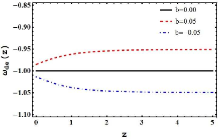
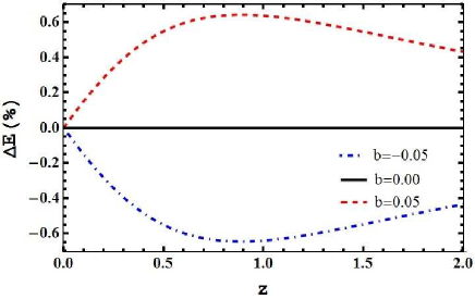
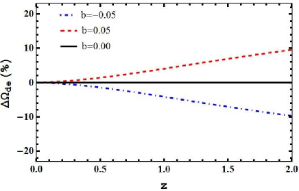
Recently, using the latest observational data that include SNIa (Suzuki et al., 2012), BAO (Blake et al., 2011b; Percival et al., 2010) and Planck CMB shift parameter (Shafer & Huterer, 2014) it has been found that , (Basilakos, 2016). These results are in agreement (within uncertainties) with those of Nesseris et al. (2013) who found , . We observe that the above analysis provide a small and negative value for but the error is quite large. In order to realize the differences of the power-law model from the cosmology at the expansion level we plot in Fig.(1) the evolution of the EoS parameter (top panel), (middle panel) and (bottom panel). Notice that the solid, dashed and dotted-dashed lines correspond to different values of the parameter, namely 0, and . Concerning the value of we have set it to which means that . Overall, the evolution of the aforementioned cosmological quantities depends on the model parameter . We verify that in the case of the effective EoS parameter of the power law model remains in the quintessence regime ( ), while it goes to phantom () for . Furthermore, from Fig.(1) (see middle and bottom panels) we observe that in the case of the cosmological quantities and of the model are large with respect to those of the reference CDM model. The opposite holds for negative values of . Regarding, the Hubble parameter we find that close to the relative deviation lies in the interval for , while the relative difference can reach up to at large redshifts .
3 growth of overdensities in gravity
In this section we explore the growth of matter over-densities in the model. First, we focus on the linear perturbation theory and then with the aid of the SCM we study the non-linear matter fluctuations.
3.1 linear growth factor
Let us start with the linear growth of non-relativistic () perturbations. In general at the sub-horizon scales matter perturbations satisfies the following differential equation
| (22) |
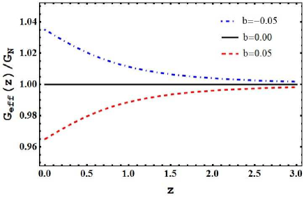
where is the effective Newton’s parameter and in the case of gravity models it takes the form (Zheng & Huang, 2011)
| (23) |
where is the Newton’s constant. Of course for Einstein’s gravity we have . Now, combining equation (16) and equation (23) we obtain
| (24) |
and utilizing a first order Taylor expansion around we find
| (25) |
Inserting equation (25) into equation (22) and changing variables from cosmic time to scale factor () we find after some calculations
| (26) |
where , and is given by equation (21). As expected for the above equation reduces to that of CDM presented in (Pace et al., 2010, and references therein).
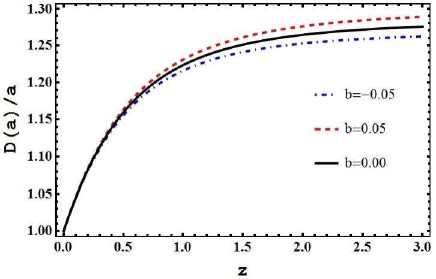
Now we numerically integrate equation (26) starting from the initial scale factor till the present epoch . Regarding the initial conditions we adopt the following case: at we use . Additionally, we also adopt the initial conditions and which guarantees that matter perturbations grow in the linear regime (see also Batista & Pace, 2013; Mehrabi et al., 2015a; Mehrabi et al., 2015b; Malekjani et al., 2017). Once the linear matter overdensity is found we compute the linear growth factor scaled to unity at the present time . In Fig.(2), we show as a function of redshift (). It is well known that for the Einstein de-Sitter (EdS) model ( the growth factor is proportional to which implies that is always equal to unity. For the concordance cosmology ( black solid curve), the growth factor is higher than the EdS model at high redshifts and progressively it starts fall down at low redshifts. The decrement of the growth factor at late times shows that the cosmological constant dominates the energy budget of the universe and consequently suppresses the growth of matter overdensities. The opposite is true at high redshifts, meaning that the effect of cosmological constant on the growth of perturbations is actually negligible and thus reaches a plateau. The above general behavior holds also for the power-law model with one difference namely, for (or -0.05) the amplitude of is somewhat larger (or lower) than the CDM model at high redshifts. Specifically, for we find that the relative difference is . Qualitatively speaking, these results are in agreement with those of DE models (see Pace et al., 2010; Devi & Sen, 2011; Pace et al., 2014a; Nazari-Pooya et al., 2016) .
3.2 The spherical collapse model
The spherical collapse model (Gunn & Gott, 1972) is a simple but still a useful tool utilized to investigate the growth of bound systems in the universe through gravitational instability (Peebles, 1993). It is well known that the main quantities of the SCM, such as the linear overdensity parameter and the virial overdensity , are affected by the presence of dark energy (Lahav et al., 1991; Wang & Steinhardt, 1998; Mota & van de Bruck, 2004; Horellou & Berge, 2005; Wang & Tegmark, 2005; Abramo et al., 2007; Basilakos & Voglis, 2007; Pace et al., 2010, 2012; Batista & Pace, 2013; Pace et al., 2014a; Pace et al., 2014b; Malekjani et al., 2015; Naderi et al., 2015). Here our aim is to extent SCM within the cosmological scenario, in order to derive the non-linear structure formation in such models and study the differences with the corresponding predictions of the usual CDM cosmology.
Since Birkhoff’s theorem holds here, we can start from the differential equation that describes the growth of matter overdensities in the non-linear regime (see also Pace et al., 2014a)
| (27) |
In the linear regime the above equation reduces to equation (22) as it should. Also, in the case of GR the full derivation of equation (22) can be found in Ref.(Abramo et al., 2007). It is interesting to mention that the non-linear matter fluctuations are affected by the law of gravity via the form of . In the case of gravity we refer the reader the work of Schaefer & Koyama (2008).
In order to understand the differences of the model from the concordance cosmology we plot in Fig. (3) a comparison of the evolution of . Notice, that the solid, dashed and the dotted-dashed curves correspond to (CDM), and . We observe that at high redshifts tends to GR (), but as we approach the present time the ratio starts to deviate from unity. As an example, at the relative deviation from GR is close to for . We also find that a positive value of implies that , while the opposite holds for .
The obvious connection between and implies that the free parameter should leave an imprint in the non-linear matter perturbations via equation (27). Indeed, using equation (25) and changing the variables from to we obtain
| (28) | |||
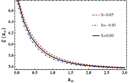
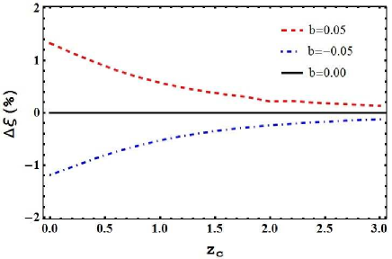
Now in order to determine and we follow the general approach of (Pace et al., 2010, 2012; Malekjani et al., 2015; Pace et al., 2014b). Specifically, regarding we utilize a two-step process. First, we numerically solve equation (28) between the epoch and the collapse redshift . As we have already mentioned in the previous section concerning the value of the initial scale factor of the universe we use . Our attempt is to calculate the initial values and for which the collapse takes place at such that (see also Malekjani et al., 2015; Nazari-Pooya et al., 2016). Second, we utilize the values for and obtained in the first step as the initial conditions for the linear equation (26) a numerical solution of which provides the critical overdensity threshold above which structures collapse . We remind the reader that in the case of the Einstein-de Sitter model is strictly equal to 1.686. In Fig. (4), we show as a function of the collapse redshift for the models explored here. We verify that converges to the Einstein de-Sitter value at high redshifts, since the matter component dominates the cosmic fluid. The critical overdensity starts to deviate from that of CDM for . In this redshift regime we observe that the critical overdensity satisfies: for and in the case of . This result is compatible with that of DE cosmologies (see Pace et al., 2010; Devi & Sen, 2011; Pace et al., 2014a; Nazari-Pooya et al., 2016) .
Furthermore we apply the following fitting function (see also Kitayama & Suto, 1996; Weinberg & Kamionkowski, 2003) to calculated in power law gravity
| (29) |
and obtain the constant coefficient in terms of parameter as
| (30) |
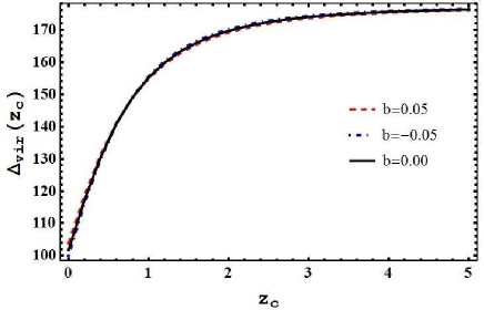
Another important quantity is the density contrast at virialization which is defined as , where is the density contrast at the turnaround point, is the normalized scale factor with respect to the turn around scale factor and is the ratio between virial radius and turn-around radius, (Wang & Steinhardt, 1998). It is well known that for the Einstein de-Sitter model we have , , and thus . However, in DE cosmologies the above quantities varies with the collapse redshift (Lahav et al., 1991; Wang & Steinhardt, 1998; Mota & van de Bruck, 2004; Horellou & Berge, 2005; Wang & Tegmark, 2005; Abramo et al., 2007; Basilakos & Voglis, 2007; Pace et al., 2010, 2012; Batista & Pace, 2013; Pace et al., 2014a; Pace et al., 2014b; Malekjani et al., 2015; Naderi et al., 2015).
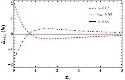
In the upper panel of Fig.(5) we plot the evolution of the density contrast at turn around. Also, in the lower panel of the same figure we present the relative difference deviation of the turn around density contrast for the power law model with respect to the solution . Obviously, the difference from the CDM case is small, namely at we find for . As expected, at very large redshifts tends to the Einstein-de Sitter value (). Moreover, in the top panel of Fig. (6) we provide as a function of and in the bottom panel of the same figure we show the behavior of . At low redshifts we find for . Therefore, in the case of positive (negative) values of we expect that the tendency for a large scale overdensity (candidate structure) is to collapse in a more (less) bound system, with respect to the CDM cosmological model.

4 Number of haloes
In this section we compute the cluster-size halo number counts within the framework of the cosmological models studied in this article. Using the Press-Schechter formalism the abundance of virialized haloes can be expressed in terms of their mass (Press & Schechter, 1974). The comoving number densities of virialized haloes with masses in the range of and is given by (Press & Schechter, 1974; Bond et al., 1991)
| (31) |
where , is the background density at the present time and is the corresponding critical density. In the standard Press-Schechter approach the mass function is Gaussian . Notice, that is the variance of the linear matter perturbations
| (32) |
where is the radius of the spherical region, is the linear power spectrum and is the Fourier transform of a spherical top-hat profile. We utilize the cold dark matter (CDM) spectrum , with the CDM transfer function according to (Eisenstein & Hu, 1998) and , following the Planck Collaboration XIII (2015) results. In this framework, the rms matter fluctuations is normalized at redshift so that for any cosmological model one has (for more detail see Basilakos et al., 2010): with
and
where the rms mass fluctuation on Mpc scales at redshift . Concerning the value of we have set it to based on the Planck 2015 results (Planck Collaboration XIV, 2016). It is worth noting that the Gaussian mass-function has a well known caveat, namely it over-predicts/under-predicts the number of low/high mass halos at the present epoch (Sheth & Tormen, 1999; Jenkins et al., 2001; Sheth & Tormen, 2002; Lima & Marassi, 2004). In order to avoid this problem in the present treatment we adopt the Sheth-Torman (ST) mass function (Sheth & Tormen, 1999, 2002):
| (33) |
Now given the determined mass range, say we can derive the halo number counts, via the integration of the expected differential halo mass function as
| (34) |
In Fig.(7), we display the expected ratio as a function of and above a limiting halo mass, which is . Concerning the upper mass limit we have set it to . We remind the reader that mass inside the radius of (Abramo et al., 2007).
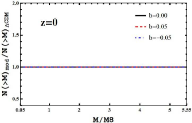

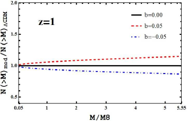
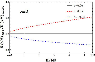
Also the panels in Fig. (7) correspond to different redshifts, namely (top left panel), (top right panel), (bottom left panel) and (bottom right panel). The results indicate that the number variation of the differences between the power law model and cosmology model is affected by variations in the value of . Considering (or ) we find that significant model differences should be expected for , with the model abundance predictions being always less (or more) than those of the corresponding cosmology. In particular, at the model with () has roughly () more (less) haloes than the standard CDM model at the low-mass tail . Obviously, as we approach the high mass haloes (see for example ) the corresponding differences become more severe. Indeed, we observe that the model with () produces () more (less) haloes with respect to those of CDM. Furthermore, the deviation between and CDM models becomes even higher at . Specifically, for the low-mass tail we find that the difference between and CDM can reach up to for , while for the high-mass end () we show that the gravity with (or -0.05) predicts (or ) more (or less) virialized haloes. We would like to point that the aforementioned predictions of the power law model are similar to those of DE models (quintessence and phantom) which adhere to GR (see Pace et al., 2014b). We have expected such a similarity because in the case of (or ) the power law model is in the quintessence (or phantom) regime, namely the effective EoS parameter obeys (or ) [see Fig. (1)].
Although our analysis is self-consistent, in the sense that we compare the expectations of model with respect to those of the concordance cosmology using the same mass function, we want to investigate how sensitive are the observational predictions to the different mass functions fitting formulas. For comparison, we use the mass function provided by Reed et al. (2007):
| (35) |
where
| (36) |
We conclude that the difference between ST mass function and Reed et al. mass function is negligible at low mass tails and low-redshifts respectively. However, as we approach the high mass tail at , we find differences between the two mass functions. Specificaly, for () the mass function of Reed et al. (2007) provides () more (less) haloes with respect to ST mass function. Overall, we verify that there are observational signatures that can be used to differentiate the power law gravity from the CDM and possibly from a large class of DE models (see also Basilakos et al., 2010; Malekjani et al., 2015).
5 conclusion
In this article, we have studied the spherical collapse model (SCM) and the number counts of massive clusters beyond the concordance cosmology by utilizing the power law model for the gravity.
First, at the level of the resulting cosmic expansion we have found that the evolution of the main cosmological quantities are affected by the power-law parameter, . In particular, for we have shown that the effective EoS parameter of the gravity is in the quintessence regime ( ), while it goes to phantom () in the case of . Concerning the Hubble parameter, we have found that the model is close to that of the CDM model (the relative difference can reach up to ), as long as they are confronted with the quoted set of observations.
Second we have investigated analytically and numerically the linear and non-linear (via SCM) regimes of the matter perturbations in the context of the current gravity. In this case we have found that the general behavior of the growth factor is similar to that of the CDM cosmological model, although the relative difference is close to at high redshifts. We have showed that at low redshidts the linear growth of matter perturbations are suppressed due to the modifications of gravity while at high redshifts the effect of modified gravity is less important. Extending the model in the non-linear phase of matter perturbations, we have computed the well known SCM parameters, namely the linear overdensity and the virial overdensity . We have showed that and are affected by the value of . As expected both quantities tend to those of Einsten-deSitter model at high redshifts. Also, we have found that the predictions of SCM model in the power law model are similar with those DE models (quintessence or phantom) which adhere to GR (for comparison see Pace et al., 2014b).
Finally, despite the fact that the model closely reproduce the CDM Hubble parameter, we have shown that the model can be differentiated from the reference cosmology on the basis of their number counts of cluster-size halos. Indeed, using the Press-Schechter formalism in the framework of Sheth-Torman (ST) mass function (Sheth & Tormen, 1999, 2002), we have found clear signs of difference, especially at , with respect to the CDM predictions. Therefore, the power-law gravity model can be distinguished from the CDM and possibly from a large class of DE models, including those of modified gravity. Also, using the mass function of Reed et al. Reed et al. (2007) we found that the difference between the two mass functions is negligible at low mass tails and low-redshifts respectively. However, as we approach the high mass tail at we found that the relative difference lies in the interval . To this end, in the light of future cluster surveys the methodology of cluster number counts appears to be very competitive towards testing the nature of dark energy on cosmological scales.
References
- Abramo et al. (2007) Abramo L. R., Batista R. C., Liberato L., Rosenfeld R., 2007, JCAP, 11, 12
- Abramo et al. (2009) Abramo L. R., Batista R. C., Liberato L., Rosenfeld R., 2009, Phys. Rev. D, 79, 023516
- Alcaniz (2004) Alcaniz J. S., 2004, Phys. Rev., D69, 083521
- Allen et al. (2004) Allen S. W., Schmidt R. W., Ebeling H., Fabian A. C., van Speybroeck L., 2004, Mon. Not. Roy. Astron. Soc., 353, 457
- Amendola et al. (2008) Amendola L., Kunz M., Sapone D., 2008, JCAP, 0804, 013
- Armendariz-Picon et al. (2001) Armendariz-Picon C., Mukhanov V., Steinhardt P. J., 2001, Phys. Rev. D, 63(10), 103510
- Ascasibar et al. (2004) Ascasibar Y., Yepes G., Gottlöber S., Müller V., 2004, MNRAS, 352, 1109
- Avila-Reese et al. (1998) Avila-Reese V., Firmani C., Hernandez X., 1998, Astrophys. J., 505, 37
- Bamba et al. (2011) Bamba K., Geng C.-Q., Lee C.-C., Luo L.-W., 2011, JCAP, 1101, 021
- Bamba et al. (2012) Bamba K., Myrzakulov R., Nojiri S., Odintsov S. D., 2012, Phys. Rev., D85, 104036
- Basilakos (2016) Basilakos S., 2016, Phys. Rev., D93, 083007
- Basilakos & Voglis (2007) Basilakos S., Voglis N., 2007, Mon. Not. Roy. Astron. Soc., 374, 269
- Basilakos et al. (2009) Basilakos S., Sanchez J. C. B., Perivolaropoulos L., 2009, Phys. Rev. D, 80, 043530
- Basilakos et al. (2010) Basilakos S., Plionis M., Lima J. A. S., 2010, Phys. Rev., D82, 083517
- Basse et al. (2011) Basse T., Bj lde O. E., Wong Y. Y. Y., 2011, JCAP, 10, 38
- Batista & Pace (2013) Batista R., Pace F., 2013, JCAP, 1306, 044
- Bengochea & Ferraro (2009) Bengochea G. R., Ferraro R., 2009, Phys. Rev., D79, 124019
- Benjamin et al. (2007) Benjamin J., et al., 2007, Mon. Not. Roy. Astron. Soc., 381, 702
- Bento et al. (2002) Bento M. C., Bertolami O., Sen A. A., 2002, Phys. Rev., D66, 043507
- Bertschinger (1985) Bertschinger E., 1985, ApJS, 58, 39
- Blake et al. (2011a) Blake C., Brough S., Colless M., Contreras C., Couch W., et al., 2011a, MNRAS, 415, 2876
- Blake et al. (2011b) Blake C., Kazin E., Beutler F., Davis T., Parkinson D., et al., 2011b, MNRAS, 418, 1707
- Bond et al. (1991) Bond J. R., Cole S., Efstathiou G., Kaiser N., 1991, ApJ, 379, 440
- Cai et al. (2016) Cai Y.-F., Capozziello S., De Laurentis M., Saridakis E. N., 2016, Rept. Prog. Phys., 79, 106901
- Caldwell (2002) Caldwell R. R., 2002, Phys. Lett. B, 545, 23
- Caldwell et al. (1998) Caldwell R. R., Dave R., Steinhardt P. J., 1998, Phys. Rev. Lett., 80, 1582
- Capozziello & Francaviglia (2008) Capozziello S., Francaviglia M., 2008, Gen. Rel. Grav., 40, 357
- Capozziello & Vignolo (2009) Capozziello S., Vignolo S., 2009, Class. Quant. Grav., 26, 175013
- Capozziello & Vignolo (2010) Capozziello S., Vignolo S., 2010, Annalen Phys., 19, 238
- Capozziello et al. (2007) Capozziello S., Stabile A., Troisi A., 2007, Phys. Rev., D76, 104019
- Capozziello et al. (2011) Capozziello S., Cardone V. F., Farajollahi H., Ravanpak A., 2011, Phys. Rev., D84, 043527
- Cardone et al. (2012) Cardone V. F., Radicella N., Camera S., 2012, Phys. Rev., D85, 124007
- Carroll (2001) Carroll S. M., 2001, Living Reviews in Relativity, 380, 1
- Chen et al. (2011) Chen S.-H., Dent J. B., Dutta S., Saridakis E. N., 2011, Phys. Rev., D83, 023508
- Chen et al. (2015) Chen Z.-C., Wu Y., Wei H., 2015, Nucl. Phys., B894, 422
- Cole et al. (2005) Cole S., et al., 2005, MNRAS, 362, 505
- Copeland et al. (2006) Copeland E. J., Sami M., Tsujikawa S., 2006, IJMP, D15, 1753
- Dent et al. (2011) Dent J. B., Dutta S., Saridakis E. N., 2011, JCAP, 1101, 009
- Devi & Sen (2011) Devi N. C., Sen A. A., 2011, Mon. Not. Roy. Astron. Soc., 413, 2371
- Einstein (1928) Einstein A., 1928, Sitz. Preuss. Akad. Wiss., p.217, ibid p. 224
- Eisenstein & Hu (1998) Eisenstein D. J., Hu W., 1998, Astrophys. J., 496, 605
- Eisenstein et al. (2005) Eisenstein D. J., et al., 2005, ApJ, 633, 560
- Elizalde et al. (2004) Elizalde E., Nojiri S., Odintsov S. D., 2004, Phys. Rev., D70, 043539
- Erickson et al. (2002) Erickson J. K., Caldwell R., Steinhardt P. J., Armendariz-Picon C., Mukhanov V. F., 2002, Phys. Rev. Lett., 88, 121301
- Fan et al. (2015) Fan Y., Wu P., Yu H., 2015, Phys. Rev., D92, 083529
- Faraoni (2010) Faraoni V., 2010, Phys. Rev., D81, 044002
- Ferraro & Fiorini (2007) Ferraro R., Fiorini F., 2007, Phys. Rev., D75, 084031
- Ferraro & Fiorini (2008) Ferraro R., Fiorini F., 2008, Phys. Rev., D78, 124019
- Fillmore & Goldreich (1984) Fillmore J. A., Goldreich P., 1984, ApJ, 281, 1
- Fu et al. (2008) Fu L., et al., 2008, Astron. Astrophys., 479, 9
- Geng & Wu (2013) Geng C.-Q., Wu Y.-P., 2013, JCAP, 1304, 033
- Geng et al. (2011) Geng C.-Q., Lee C.-C., Saridakis E. N., Wu Y.-P., 2011, Phys. Lett., B704, 384
- Geng et al. (2012) Geng C.-Q., Lee C.-C., Saridakis E. N., 2012, JCAP, 1201, 002
- Gunn & Gott (1972) Gunn J. E., Gott J. R., 1972, ApJ, 176, 1
- Hayashi & Shirafuji (1979) Hayashi K., Shirafuji T., 1979, Phys. Rev., D19, 3524
- Hoffman & Shaham (1985) Hoffman Y., Shaham J., 1985, ApJ, 297, 16
- Horellou & Berge (2005) Horellou C., Berge J., 2005, MNRAS, 360, 1393
- Iorio et al. (2015) Iorio L., Radicella N., Ruggiero M. L., 2015, JCAP, 1508, 021
- Izumi & Ong (2013) Izumi K., Ong Y. C., 2013, JCAP, 1306, 029
- Jarosik et al. (2011) Jarosik N., et al., 2011, ApJS, 192, 14
- Jenkins et al. (2001) Jenkins A., Frenk C. S., White S. D. M., Colberg J. M., Cole S., Evrard A. E., Couchman H. M. P., Yoshida N., 2001, Mon. Not. Roy. Astron. Soc., 321, 372
- Kamenshchik et al. (2001) Kamenshchik A. Yu., Moschella U., Pasquier V., 2001, Phys. Lett., B511, 265
- Karami et al. (2013) Karami K., Abdolmaleki A., Asadzadeh S., Safari Z., 2013, Eur. Phys. J., C73, 2565
- Kitayama & Suto (1996) Kitayama T., Suto Y., 1996, Astrophys. J., 469, 480
- Komatsu et al. (2009) Komatsu E., Dunkley J., Nolta M. R., et al. 2009, ApJS, 180, 330
- Komatsu et al. (2011) Komatsu E., Smith K. M., Dunkley J., et al. 2011, ApJS, 192, 18
- Kowalski et al. (2008) Kowalski M., Rubin D., Aldering G., et al. 2008, ApJ, 686, 749
- Lahav et al. (1991) Lahav O., Lilje P. B., Primack J. R., Rees M. J., 1991, MNRAS, 251, 128
- Li et al. (2009) Li M., Li X. D., Wang S., Zhang X., 2009, J. Cosmology Astropart. Phys., 6, 036
- Li et al. (2011) Li B., Sotiriou T. P., Barrow J. D., 2011, Phys. Rev., D83, 104017
- Lima & Marassi (2004) Lima J. A. S., Marassi L., 2004, Int. J. Mod. Phys., D13, 1345
- Linder (2010) Linder E. V., 2010, Phys. Rev., D81, 127301
- Malekjani et al. (2015) Malekjani M., Naderi T., Pace F., 2015, Mon. Not. Roy. Astron. Soc., 453, 4148
- Malekjani et al. (2017) Malekjani M., Basilakos S., Davari Z., Mehrabi A., Rezaei M., 2017, Mon. Not. Roy. Astron. Soc., 464, 1192
- Maluf (1994) Maluf J. W., 1994, J. Math. Phys., 35, 335
- Maor & Lahav (2005) Maor I., Lahav O., 2005, JCAP, 7, 3
- Mehrabi et al. (2015a) Mehrabi A., Basilakos S., Pace F., 2015a, MNRAS, 452, 2930
- Mehrabi et al. (2015b) Mehrabi A., Basilakos S., Malekjani M., Davari Z., 2015b, Phys. Rev., D92, 123513
- Mehrabi et al. (2017) Mehrabi A., Pace F., Malekjani M., Del Popolo A., 2017, Mon. Not. Roy. Astron. Soc., 465(3), 2687
- Meng & Wang (2011) Meng X.-h., Wang Y.-b., 2011, Eur. Phys. J., C71, 1755
- Mota & van de Bruck (2004) Mota D. F., van de Bruck C., 2004, A&A, 421, 71
- Myrzakulov (2011) Myrzakulov R., 2011, Eur. Phys. J., C71, 1752
- Naderi et al. (2015) Naderi T., Malekjani M., Pace F., 2015, MNRAS, 447, 1873
- Nazari-Pooya et al. (2016) Nazari-Pooya N., Malekjani M., Pace F., Jassur D. M.-Z., 2016, Mon. Not. Roy. Astron. Soc., 458, 3795
- Nesseris et al. (2013) Nesseris S., Basilakos S., Saridakis E. N., Perivolaropoulos L., 2013, Phys. Rev., D88, 103010
- Nojiri & Odintsov (2011) Nojiri S., Odintsov S. D., 2011, Phys. Rept., 505, 59
- Nunes et al. (2016) Nunes R. C., Pan S., Saridakis E. N., 2016, JCAP, 1608, 011
- Pace et al. (2010) Pace F., Waizmann J. C., Bartelmann M., 2010, MNRAS, 406, 1865
- Pace et al. (2012) Pace F., Fedeli C., Moscardini L., Bartelmann M., 2012, MNRAS, 422, 1186
- Pace et al. (2014a) Pace F., Moscardini L., Crittenden R., Bartelmann M., Pettorino V., 2014a, Mon. Not. Roy. Astron. Soc., 437, 547
- Pace et al. (2014b) Pace F., Batista R. C., Del Popolo A., 2014b, MNRAS, 445, 648
- Padmanabhan (2002) Padmanabhan T., 2002, Phys. Rev. D, 66, 021301
- Padmanabhan (2003) Padmanabhan T., 2003, Phys. Rep., 380, 235
- Peebles (1993) Peebles P. J. E., 1993, Principles of physical cosmology. Princeton University Press
- Peebles & Ratra (2003) Peebles P. J., Ratra B., 2003, Reviews of Modern Physics, 75, 559
- Percival et al. (2010) Percival W. J., Reid B. A., Eisenstein D. J., et al. 2010, MNRAS, 401, 2148
- Perlmutter et al. (1999) Perlmutter S., Aldering G., Goldhaber G., et al. 1999, ApJ, 517, 565
- Planck Collaboration XIII (2015) Planck Collaboration XIII 2015, ArXiv e-prints, 1502.01589
- Planck Collaboration XIV (2016) Planck Collaboration XIV 2016, Astron.Astrophys., 594, A14
- Press & Schechter (1974) Press W. H., Schechter P., 1974, ApJ, 187, 425
- Reed et al. (2007) Reed D., Bower R., Frenk C., Jenkins A., Theuns T., 2007, Mon. Not. Roy. Astron. Soc., 374, 2
- Reid et al. (2012) Reid B. A., Samushia L., White M., Percival W. J., Manera M., et al., 2012, MNRAS, 426, 2719
- Riess et al. (1998) Riess A. G., Filippenko A. V., Challis P., et al. 1998, AJ, 116, 1009
- Ryden & Gunn (1987) Ryden B. S., Gunn J. E., 1987, ApJ, 318, 15
- Saez-Gomez et al. (2016) Saez-Gomez D., Carvalho C. S., Lobo F. S. N., Tereno I., 2016, Phys. Rev., D94, 024034
- Sahni & Starobinsky (2000) Sahni V., Starobinsky A. A., 2000, IJMPD, 9, 373
- Schaefer & Koyama (2008) Schaefer B. M., Koyama K., 2008, Mon. Not. Roy. Astron. Soc., 385, 411
- Shafer & Huterer (2014) Shafer D. L., Huterer D., 2014, Phys. Rev., D89, 063510
- Sharif & Rani (2013) Sharif M., Rani S., 2013, Astrophys. Space Sci., 345
- Sheth & Tormen (1999) Sheth R. K., Tormen G., 1999, MNRAS, 308, 119
- Sheth & Tormen (2002) Sheth R. K., Tormen G., 2002, MNRAS, 329, 61
- Sotiriou & Faraoni (2010) Sotiriou T. P., Faraoni V., 2010, Rev. Mod. Phys., 82, 451
- Subramanian et al. (2000) Subramanian K., Cen R., Ostriker J. P., 2000, ApJ, 538, 528
- Suzuki et al. (2012) Suzuki N., Rubin D., Lidman C., Aldering G., et.al 2012, ApJ, 746, 85
- Tegmark et al. (2004) Tegmark M., et al., 2004, Phys. Rev. D, 69, 103501
- Wang & Steinhardt (1998) Wang L., Steinhardt P. J., 1998, ApJ, 508, 483
- Wang & Tegmark (2005) Wang Y., Tegmark M., 2005, Phys. Rev. D, 71, 103513
- Wei (2012) Wei H., 2012, Phys. Lett., B712, 430
- Wei et al. (2012) Wei H., Qi H.-Y., Ma X.-P., 2012, Eur. Phys. J., C72, 2117
- Weinberg (1989) Weinberg S., 1989, Reviews of Modern Physics, 61, 1
- Weinberg & Kamionkowski (2003) Weinberg N. N., Kamionkowski M., 2003, Mon. Not. Roy. Astron. Soc., 341, 251
- Williams et al. (2004) Williams L. L. R., Babul A., Dalcanton J. J., 2004, ApJ, 604, 18
- Wintergerst & Pettorino (2010) Wintergerst N., Pettorino V., 2010, Phys. Rev. D., 82, 103516
- Wu & Geng (2012a) Wu Y.-P., Geng C.-Q., 2012a, JHEP, 11, 142
- Wu & Geng (2012b) Wu Y.-P., Geng C.-Q., 2012b, Phys. Rev., D86, 104058
- Wu & Yu (2010a) Wu P., Yu H. W., 2010a, Phys. Lett., B692, 176
- Wu & Yu (2010b) Wu P., Yu H. W., 2010b, Phys. Lett., B693, 415
- Wu & Yu (2011) Wu P., Yu H. W., 2011, Eur. Phys. J., C71, 1552
- Yerzhanov et al. (2010) Yerzhanov K. K., Myrzakul S. R., Kulnazarov I. I., Myrzakulov R., 2010
- Zhang et al. (2011) Zhang Y., Li H., Gong Y., Zhu Z.-H., 2011, JCAP, 1107, 015
- Zheng & Huang (2011) Zheng R., Huang Q.-G., 2011, JCAP, 1103, 002