The square lattice Ising model on the rectangle
I: Finite systems

Abstract

The partition function of the square lattice Ising model on the rectangle with open boundary conditions in both directions is calculated exactly for arbitrary system size $L\times M$ and temperature. We start with the dimer method of Kasteleyn, McCoy & Wu, construct a highly symmetric block transfer matrix and derive a factorization of the involved determinant, effectively decomposing the free energy of the system into two parts, $F(L,M)=F_{\mathrm{strip}}(L,M)+F_{\mathrm{strip}}^{\mathrm{res}}(L,M)$, where the residual part $F_{\mathrm{strip}}^{\mathrm{res}}(L,M)$ contains the nontrivial finite-$L$ contributions for fixed $M$. It is given by the determinant of a $\nicefrac{{M}}{{2}}\times\nicefrac{{M}}{{2}}$ matrix and can be mapped onto an effective spin model with $M$ Ising spins and long-range interactions. While $F_{\mathrm{strip}}^{\mathrm{res}}(L,M)$ becomes exponentially small for large $L/M$ or off-critical temperatures, it leads to important finite-size effects such as the critical Casimir force near criticality. The relations to the Casimir potential and the Casimir force are discussed.

I Introduction

The two-dimensional Ising model Ising25 on the $L\times M$ square lattice is one of the best investigated models in statistical mechanics. After the exact solution of the periodic case by Onsager Onsager44 , many authors have contributed to the knowledge about this model under various aspects, such as different boundary conditions (BCs) or surface effects McCoyWu73 ; Baxter82 . Near the critical temperature $T_{\mathrm{c}}$, where the correlation length $\xi(T)$ of thermal fluctuations becomes of the order of the system size $L$ or $M$ in finite systems, interesting finite-size effects such as the critical Casimir effect emerge, which describes an interaction of the system boundaries mediated by long-range critical fluctuations FisherdeGennes78 in close analogy to the quantum electrodynamical Casimir effect Casimir48 . These finite-size effects can be described by universal finite-size scaling functions, that only depend on the bulk and surface universality classes of the model, as well as on the BCs and on the system shape. They have been calculated exactly for many cases, albeit mostly in strip geometry, where the aspect ratio $\rho=L/M$ of the system goes to zero EvansStecki94 ; Au-YangFisher80 ; BrankovDantchevTonchev00 . Directly at the critical point, exact methods or conformal field theory can be used to get exact expressions for the Casimir amplitude $\Delta_{\mathrm{C}}(\rho)$ for arbitrary $\rho$. This has been done for periodic FerdinandFisher69 ; LuWu01 as well as for open BCs KlebanVassileva91 . At arbitrary aspect ratios and temperatures, however, the finite-size scaling functions must be derived from the exact solution of the system with the correct BC. For the Ising model, this has been done only in a few cases, namely for the torus with periodic BCs in both directions HuchtGruenebergSchmidt11 ; HobrechtHucht16a and for the cylinder with open BCs in one direction HobrechtHucht16a .

In this work and in the forthcoming publication Hucht16b we will present a calculation of these finite-size contributions, namely the residual free energy also denoted Casimir potential, as well as the resulting critical Casimir forces, for open BCs at arbitrary temperatures $T$ and system size $L\times M$. In order to calculate these quantities correctly, all infinite volume free energies, i. e., the bulk free energy $LMf_{\mathrm{b}}(T)$, the surface free energies $Lf_{\mathrm{s}}^{\leftrightarrow}(T)$ and $Mf_{\mathrm{s}}^{\updownarrow}(T)$ in the two directions $\leftrightarrow$ and $\updownarrow$, as well as the corner free energy $f_{\mathrm{c}}(T)$ must be known and subtracted from the free energy of the finite system. While the bulk and surface free energies are known for a long time Onsager44 ; McCoyWu73 , the corner free energy $f_{\mathrm{c}}(T)$ was only known below $T_{\mathrm{c}}$ from a conjecture by Vernier & Jacobsen VernierJacobsen12 . The corresponding product formula for the paramagnetic phase is given in the Appendix of this work and will be discussed in Hucht16b .

In a recent preprint Baxter16 , Rodney J. Baxter presented an exact calculation of the infinite volume corner free energy $f_{\mathrm{c}}(T)$ in the ordered phase $T<T_{\mathrm{c}}$, verifying the conjecture of Vernier & Jacobsen. In this manuscript we present a calculation within the same model and geometry and discuss the similarities and differences. While Baxter focused on the corner free energy contribution $f_{\mathrm{c}}(T)$ in the thermodynamic limit, the focus of this work is on the exact finite-size corrections to the free energy at arbitrary system size and temperature.

We start the present calculation with the Pfaffian formulation of Kasteleyn, McCoy & Wu Kasteleyn63 ; McCoyWu73 in cylinder geometry and reduce the involved determinant of a sparse $4LM\times 4LM$ matrix to the determinant of a $LM\times LM$ block-tridiagonal matrix using an appropriate Schur complement. This determinant can then be calculated with the formula of Molinari Molinari08 , introducing $2\times 2$ block transfer matrices $\bm{\mathrm{\mathcal{T}}}_{\negmedspace\ell}$ with $M\times M$ blocks. Up to here the calculation is done for arbitrary local couplings $K_{\ell,m}^{\leftrightarrow}$ and $K_{\ell,m}^{\updownarrow}$ in the two directions on the cylinder. Then we assume open BCs in both directions and homogeneous, albeit anisotropic couplings $K^{\leftrightarrow}$ and $K^{\updownarrow}$. After that simplification the partition function $Z$ is of the form $Z^{2}\propto\det\langle\bm{\mathrm{1}}\,\bm{\mathrm{0}}|\bm{\mathrm{\mathcal{T}}}^{L}|\bm{\mathrm{1}}\,\bm{\mathrm{0}}\rangle$, in strong analogy to Baxter’s result Baxter16 .

While Baxter at this point performs the thermodynamic limit $L\to\infty$ with fixed $M$, neglecting the finite-$L$ contributions, we are able to proceed and further reduce the size of the involved matrices. The block transfer matrix $\bm{\mathrm{\mathcal{T}}}$ can be symmetrized and block diagonalized such that its eigenvalues $\lambda$ are real and occur in pairs $(\lambda,\lambda^{-1})$, and the calculation is simplified by the introduction of the natural angle variable $\varphi$, leading to the characteristic polynomial $P_{M}(\varphi)$. It turns out that the eigenvalues $\lambda$ are directly related to the well-known Onsager-$\gamma$ via $\gamma=\log\lambda$.

The eigenvectors $\vec{X}$ of $\bm{\mathrm{\mathcal{T}}}$ show an important symmetry with respect to the mapping $\lambda\leftrightarrow\lambda^{-1}$, which can eventually be used to reduce the involved matrices from $2M\times 2M$ to $M\times M$ and, more important, to factorize the determinant into a product of the form $\det(\bm{\mathrm{W}}^{T}\bm{\mathrm{D}}\bm{\mathrm{W}})=\det^{2}\bm{\mathrm{W}}\det\bm{\mathrm{D}}$, where $\bm{\mathrm{D}}$ is diagonal.

The remaining matrix $\bm{\mathrm{W}}$ is of Vandermonde type and can be considerably simplified using the invariance property of Vandermonde determinants with respect to basis transformations. Using the well known product formula for these determinants the matrix size can be further reduced to $\nicefrac{{M}}{{2}}\times\nicefrac{{M}}{{2}}$. We show that this determinant contains all remaining nontrivial finite-size contributions, and discuss the different resulting contributions to the free energy.

Finally we present an exact mapping of the remaining determinant onto a long-range spin model with $M$ spins and logarithmic interactions in an effective magnetic field of strength $L$, which might give rise to an alternative calculation of the remaining determinant. We conclude with a discussion of the results.

In the second part of this work Hucht16b , which will be published separately, we perform the finite-size scaling limit $L,M\to\infty$, $T\to T_{\mathrm{c}}$ with fixed temperature scaling variable $x\propto(T/T_{\mathrm{c}}-1)M$ and fixed aspect ratio $\rho$. After a number of simplifications, we derive exponentially fast converging series for the Casimir scaling functions. At the critical point $T=T_{\mathrm{c}}$ we can rewrite the Casimir amplitude $\Delta_{\mathrm{C}}(\rho)$ in terms of the Dedekind eta function, confirming a prediction from conformal field theory KlebanVassileva91 .

II Model and Pfaffian representation

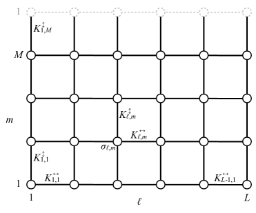
Figure 1: The square lattice with cylinder geometry for $M=4$ and $L=6$.

We consider the Ising model on the square lattice with $L$ columns and $M$ rows as shown in figure 1, and start with arbitrary reduced (in units of $k_{\mathrm{B}}T$, with Boltzmann constant $k_{\mathrm{B}}$) couplings $K_{\ell,m}^{\leftrightarrow}$ and $K_{\ell,m}^{\updownarrow}$ in horizontal and vertical direction on the cylinder periodic in vertical ($M$) direction. Our aim is to calculate the partition function

$$Z=\operatorname{Tr}\exp\sum_{\ell=1}^{L}\sum_{m=1}^{M}\left(K_{\ell,m}^{\leftrightarrow}\sigma_{\ell,m}\sigma_{\ell+1,m}+K{}_{\ell,m}^{\updownarrow}\sigma_{\ell,m}\sigma_{\ell,m+1}\right),$$ (1)

where the trace is over all $2^{LM}$ configurations of the $LM$ spins $\sigma_{\ell,m}=\pm 1$, with $\sigma_{L+1,m}=0$ and $\sigma_{\ell,M+1}=\sigma_{\ell,1}$. We assume open BC in horizontal ($L$) direction, $K_{L,m}^{\leftrightarrow}=0$, and first derive a transfer matrix formulation for this general case. After that we focus on the rectangular homogeneous case, $K_{\ell,M}^{\updownarrow}=0$, $K_{\ell,m<M}^{\updownarrow}=K^{\updownarrow}$, $K_{\ell<L,m}^{\leftrightarrow}=K^{\leftrightarrow}$, where we still allow for anisotropic couplings.

Our starting point is the Pfaffian representation by Kasteleyn, McCoy & Wu Kasteleyn63 ; McCoyWu73 , where the partition function in cylinder geometry is given by

$$Z=\sqrt{C_{0}}\,\operatorname{Pf}\bm{\mathrm{\mathcal{A}}}=\sqrt{C_{0}\det\bm{\mathrm{\mathcal{A}}}}\,,$$ (2)

with the constant

$$C_{0} \equiv 4^{LM}\prod_{\ell=1}^{L-1}\prod_{m=1}^{M}\cosh^{2}K_{\ell,m}^{\leftrightarrow}\;\prod_{\ell=1}^{L}\prod_{m=1}^{M}\cosh^{2}K_{\ell,m}^{\updownarrow}.$$ (3)

We define the antisymmetric $4LM\times 4LM$ sparse matrix $\bm{\mathrm{\mathcal{A}}}$ as a $4\times 4$ block matrix (the bar denotes transposition, “$\equiv$” denotes a definition)

$$\bm{\mathrm{\mathcal{A}}}\equiv\begin{bmatrix}\bm{\mathrm{0}}&\bm{\mathrm{1}}+\bm{\mathrm{Z}}^{\updownarrow}&-\bm{\mathrm{1}}&-\bm{\mathrm{1}}\\ -\bm{\mathrm{1}}-\bar{\bm{\mathrm{Z}}}^{\updownarrow}&\bm{\mathrm{0}}&\bm{\mathrm{1}}&-\bm{\mathrm{1}}\\ \bm{\mathrm{1}}&-\bm{\mathrm{1}}&\bm{\mathrm{0}}&\bm{\mathrm{1}}+\bm{\mathrm{Z}}^{\leftrightarrow}\\ \bm{\mathrm{1}}&\bm{\mathrm{1}}&-\bm{\mathrm{1}}-\bar{\bm{\mathrm{Z}}}^{\leftrightarrow}&\bm{\mathrm{0}}\end{bmatrix},$$ (4)

where the $LM\times LM$ matrices $\bm{\mathrm{Z}}^{\delta}$ contain the couplings $z_{\ell,m}^{\delta}\equiv\tanh K_{\ell,m}^{\delta}$ in direction $\delta=\,\leftrightarrow,\updownarrow$ via the $M\times M$ and $LM\times LM$ diagonal matrices

$$\bm{\mathrm{z}}_{\ell}^{\delta}\equiv\operatorname{\mathbf{diag}}(z_{\ell,1}^{\delta},\ldots,z_{\ell,M}^{\delta}),\quad\bm{\mathrm{z}}^{\delta}\equiv\operatorname{\mathbf{diag}}(\bm{\mathrm{z}}_{1}^{\delta},\ldots,\bm{\mathrm{z}}_{L}^{\delta}),$$ (5)

according to

$$\bm{\mathrm{Z}}^{\leftrightarrow} \equiv\bm{\mathrm{z}}^{\leftrightarrow}(\bm{\mathrm{H}}_{L}^{0}\otimes\bm{\mathrm{1}}_{M}),$$ (6a)

$$\bm{\mathrm{Z}}^{\updownarrow} \equiv\bm{\mathrm{z}}^{\updownarrow}(\bm{\mathrm{1}}_{L}\otimes\bm{\mathrm{H}}_{M}^{-})=\operatorname{\mathbf{diag}}(\bm{\mathrm{z}}_{1}^{\updownarrow}\bm{\mathrm{H}}_{M}^{-},\ldots,\bm{\mathrm{z}}_{L}^{\updownarrow}\bm{\mathrm{H}}_{M}^{-}).$$ (6b)

Here we have introduced the $n\times n$ shift matrices

$$\bm{\mathrm{H}}_{n}^{0}\equiv\begin{pmatrix}0&1\\ &\ddots&\ddots\\ &&\ddots&1\\ 0&&&0\end{pmatrix},\quad\bm{\mathrm{H}}_{n}^{-}\equiv\begin{pmatrix}0&1\\ &\ddots&\ddots\\ &&\ddots&1\\ -1&&&0\end{pmatrix},$$ (7)

that, together with the $n\times n$ identity matrix $\bm{\mathrm{1}}_{n}$, define the lattice structure. We drop the index $n$ from unit and zero matrices $\bm{\mathrm{1}}$, $\bm{\mathrm{0}}$ as long as it can be implied from the context.

III Schur reduction

We first reduce the matrix size from $4LM\times 4LM$ to $LM\times LM$ by a standard Schur reduction according to

$$\det\bm{\mathrm{\mathcal{A}}}=\det\bm{\mathrm{\mathcal{A}}}_{\bar{i},\bar{i}}\det\bm{\mathrm{\mathcal{C}}}_{i,i},$$ (8)

where $\bar{i}$ denotes the index complement of $i$, i. e. $\bm{\mathrm{\mathcal{A}}}_{\bar{i},j}$ is derived from $\bm{\mathrm{\mathcal{A}}}$ by dropping row $i$ and taking column $j$. We choose $i=4$ to find, for even $M$,

$$\det\bm{\mathrm{\mathcal{A}}}_{\bar{4},\bar{4}}=\prod_{\ell=1}^{L}\Bigg{(}\prod_{{m=1\atop m\,\mathrm{odd}}}^{M-1}z_{\ell,m}^{\updownarrow}+\prod_{{m=2\atop m\,\mathrm{even}}}^{M}z_{\ell,m}^{\updownarrow}\Bigg{)}^{2}$$ (9)

as well as the $LM\times LM$ Schur complement

$$\bm{\mathrm{\mathcal{C}}}_{4,4}\equiv\bm{\mathrm{\mathcal{A}}}/\bm{\mathrm{\mathcal{A}}}_{\bar{4},\bar{4}}\equiv\bm{\mathrm{\mathcal{A}}}_{4,4}^{\vphantom{-1}}-\bm{\mathrm{\mathcal{A}}}_{4,\bar{4}}^{\vphantom{-1}}\bm{\mathrm{\mathcal{A}}}_{\bar{4},\bar{4}}^{-1}\bm{\mathrm{\mathcal{A}}}_{\bar{4},4}^{\vphantom{-1}},$$ (10)

which is antisymmetric and block tridiagonal,

$$\bm{\mathrm{\mathcal{C}}}_{4,4}=\begin{bmatrix}\bm{\mathrm{A}}_{1}&\bm{\mathrm{B}}_{1}\\ -\bar{\bm{\mathrm{B}}}_{1}&\ddots&\ddots\\ &\ddots&\ddots&\bm{\mathrm{B}}_{L-1}\\ &&-\bar{\bm{\mathrm{B}}}_{L-1}&\bm{\mathrm{A}}_{L}\end{bmatrix},$$ (11)

with $M\times M$ matrices $\bm{\mathrm{A}}_{\ell}$ and $\bm{\mathrm{B}}_{\ell}$. We also could have chosen $i=3$ for the reduction, which would reflect the matrix $\bm{\mathrm{\mathcal{C}}}_{i,i}$ along the anti-diagonal, whereas the indices $i=1,2$ do not lead to block tridiagonal matrices $\bm{\mathrm{\mathcal{C}}}_{i,i}$. The explicit expressions for the matrices $\bm{\mathrm{A}}_{\ell}$ and $\bm{\mathrm{B}}_{\ell}$ are

$$\bm{\mathrm{B}}_{\ell}^{-1} =-(\bm{\mathrm{z}}_{\ell}^{\leftrightarrow})^{-1}\bm{\mathrm{D}}_{\ell},$$ (12a)

$$\bm{\mathrm{A}}_{1} =\bm{\mathrm{A}}_{1}^{-},$$ (12b)

$$\bm{\mathrm{A}}_{\ell>1} =\bm{\mathrm{A}}_{\ell}^{-}+\bm{\mathrm{z}}_{\ell-1}^{\leftrightarrow}\bm{\mathrm{A}}_{\ell-1}^{+}\bm{\mathrm{z}}_{\ell-1}^{\leftrightarrow},$$ (12c)

with the auxiliary matrices

$$\bm{\mathrm{A}}_{\ell}^{\pm} \equiv\pm\left[(\bm{\mathrm{1}}\pm\bar{\bm{\mathrm{Z}}}_{\ell}^{\updownarrow})^{-1}-(\bm{\mathrm{1}}\pm\bm{\mathrm{Z}}_{\ell}^{\updownarrow})^{-1}\right]^{-1},$$ (13a)

$$\bm{\mathrm{D}}_{\ell} \equiv(\bm{\mathrm{1}}-\bar{\bm{\mathrm{Z}}}_{\ell}^{\updownarrow})(\bm{\mathrm{1}}-\bm{\mathrm{Z}}_{\ell}^{\updownarrow}\bar{\bm{\mathrm{Z}}}_{\ell}^{\updownarrow})^{-1}-(\bm{\mathrm{1}}-\bm{\mathrm{Z}}_{\ell}^{\updownarrow})(\bm{\mathrm{1}}-\bar{\bm{\mathrm{Z}}}_{\ell}^{\updownarrow}\bm{\mathrm{Z}}_{\ell}^{\updownarrow})^{-1},$$ (13b)

where $$\bm{\mathrm{Z}}_{\ell}^{\updownarrow}=\bm{\mathrm{z}}_{\ell}^{\updownarrow}\bm{\mathrm{H}}_{M}^{-} \bm{\mathrm{B}}_{\ell} \det\bm{\mathrm{\mathcal{C}}}_{4,4}$$ from (6b). As the matrices are invertible, the remaining determinant can be calculated with a transfer matrix approach.

IV The block transfer matrix $\bm{\mathrm{\mathcal{T}}}$

The determinant of the block tridiagonal matrix $\bm{\mathrm{\mathcal{C}}}_{4,4}$ from (11) can be calculated with the method of Molinari Molinari08 . We introduce the $2\times 2$ block transfer matrix (TM)

$$\bm{\mathrm{\mathcal{T}}}_{\ell,\ell-1}^{\ddagger}\equiv\begin{bmatrix}-\bm{\mathrm{B}}_{\ell}^{-1}\bm{\mathrm{A}}_{\ell}&\bm{\mathrm{B}}_{\ell}^{-1}\bar{\bm{\mathrm{B}}}_{\ell-1}\\ \bm{\mathrm{1}}&\bm{\mathrm{0}}\end{bmatrix},$$ (14)

with $\ell=1,\ldots,L$, and formally define $\bm{\mathrm{B}}_{0}$ and $\bm{\mathrm{B}}_{L}$, with $\bm{\mathrm{z}}_{0}^{\delta}=\bm{\mathrm{z}}_{L}^{\updownarrow}=\bm{\mathrm{0}}$ and $\bm{\mathrm{z}}_{L}^{\leftrightarrow}=\bm{\mathrm{1}}$, in order to keep the expressions simple. We can factorize $\bm{\mathrm{\mathcal{T}}}_{\ell,\ell-1}^{\ddagger}$ into two parts depending on $\ell$ and $\ell-1$, respectively,

$$\bm{\mathrm{\mathcal{T}}}_{\ell,\ell-1}^{\ddagger}=\begin{bmatrix}(\bm{\mathrm{z}}_{\ell}^{\leftrightarrow})^{-1}\bm{\mathrm{D}}_{\ell}\bm{\mathrm{A}}_{\ell}^{-}&(\bm{\mathrm{z}}_{\ell}^{\leftrightarrow})^{-1}\bm{\mathrm{D}}_{\ell}\\ \bm{\mathrm{1}}&\bm{\mathrm{0}}\end{bmatrix}\begin{bmatrix}\bm{\mathrm{1}}&\bm{\mathrm{0}}\\ \bm{\mathrm{z}}_{\ell-1}^{\leftrightarrow}\bm{\mathrm{A}}_{\ell-1}^{+}\bm{\mathrm{z}}_{\ell-1}^{\leftrightarrow}&\bm{\mathrm{z}}_{\ell-1}^{\leftrightarrow}\bar{\bm{\mathrm{D}}}_{\ell-1}^{-1}\end{bmatrix}\equiv\bm{\mathrm{\mathcal{T}}}_{\ell}^{(1)}\bm{\mathrm{\mathcal{T}}}_{\ell-1}^{(2)},$$ (15)

and we observe that in the product of TMs, $\cdots\bm{\mathrm{\mathcal{T}}}_{\ell+1,\ell}^{\ddagger}\bm{\mathrm{\mathcal{T}}}_{\ell,\ell-1}^{\ddagger}\cdots=\cdots\bm{\mathrm{\mathcal{T}}}_{\ell+1}^{(1)}\bm{\mathrm{\mathcal{T}}}_{\ell}^{(2)}\bm{\mathrm{\mathcal{T}}}_{\ell}^{(1)}\bm{\mathrm{\mathcal{T}}}_{\ell-1}^{(2)}\cdots$, we can identify a shifted TM $\bm{\mathrm{\mathcal{T}}}_{\ell}^{\dagger}\equiv\bm{\mathrm{\mathcal{T}}}_{\ell}^{(2)}\bm{\mathrm{\mathcal{T}}}_{\ell}^{(1)}$, depending only on $\ell$, with the factorization

$$\bm{\mathrm{\mathcal{T}}}_{\ell}^{\dagger}\equiv\bm{\mathrm{\mathcal{T}}}_{\ell}^{(2)}\bm{\mathrm{\mathcal{T}}}_{\ell}^{(1)}=\begin{bmatrix}(\bm{\mathrm{z}}_{\ell}^{\leftrightarrow})^{-1}&\bm{\mathrm{0}}\\ \bm{\mathrm{0}}&\bm{\mathrm{z}}_{\ell}^{\leftrightarrow}\end{bmatrix}\begin{bmatrix}\bm{\mathrm{1}}&\bm{\mathrm{0}}\\ \bm{\mathrm{A}}_{\ell}^{+}&\bm{\mathrm{1}}\end{bmatrix}\begin{bmatrix}\bm{\mathrm{0}}&\bm{\mathrm{D}}_{\ell}\\ \bar{\bm{\mathrm{D}}}_{\ell}^{-1}&\bm{\mathrm{0}}\end{bmatrix}\begin{bmatrix}\bm{\mathrm{1}}&\bm{\mathrm{0}}\\ \bm{\mathrm{A}}_{\ell}^{-}&\bm{\mathrm{1}}\end{bmatrix}.$$ (16)

Using a block rotation by $\theta=\pi/4$, with

$$\bm{\mathrm{R}}_{\theta}\equiv\bm{\mathrm{r}}_{\theta}\otimes\bm{\mathrm{1}},\qquad\bm{\mathrm{r}}_{\theta}\equiv\begin{pmatrix}\cos\theta&\sin\theta\\ -\sin\theta&\cos\theta\end{pmatrix},$$ (17)

we find the simple representation

$$\bar{\bm{\mathrm{R}}}_{\frac{\pi}{4}}\begin{bmatrix}\bm{\mathrm{1}}&\bm{\mathrm{0}}\\ \bm{\mathrm{A}}_{\ell}^{+}&\bm{\mathrm{1}}\end{bmatrix}\begin{bmatrix}\bm{\mathrm{0}}&\bm{\mathrm{D}}_{\ell}\\ \bar{\bm{\mathrm{D}}}_{\ell}^{-1}&\bm{\mathrm{0}}\end{bmatrix}\begin{bmatrix}\bm{\mathrm{1}}&\bm{\mathrm{0}}\\ \bm{\mathrm{A}}_{\ell}^{-}&\bm{\mathrm{1}}\end{bmatrix}\bm{\mathrm{R}}_{\frac{\pi}{4}}=\begin{bmatrix}\bar{\bm{\mathrm{H}}}^{-}&\bm{\mathrm{0}}\\ \bm{\mathrm{0}}&\bm{\mathrm{1}}\end{bmatrix}\begin{bmatrix}\bm{\mathrm{t}}_{\ell,+}&\bm{\mathrm{t}}_{\ell,-}\\ \bm{\mathrm{t}}_{\ell,-}&\bm{\mathrm{t}}_{\ell,+}\end{bmatrix}\begin{bmatrix}\bm{\mathrm{H}}^{-}&\bm{\mathrm{0}}\\ \bm{\mathrm{0}}&\bm{\mathrm{1}}\end{bmatrix}\equiv\bm{\mathrm{\mathcal{V}}}_{\ell}^{\updownarrow},$$ (18)

where the matrices

$$\bm{\mathrm{t}}_{\ell}\equiv\operatorname{\mathbf{diag}}(t_{\ell,1},\ldots,t_{\ell,M})$$ (19)

contain the dual couplings $t\equiv z^{\updownarrow\,*}=\frac{1-z^{\updownarrow}}{1+z^{\updownarrow}}$ of $z^{\updownarrow}$. We have introduced the abbreviation

$$a_{\pm}\equiv{\textstyle\frac{1}{2}}(a\pm a^{-1}),$$ (20)

such that $a^{\pm 1}=a_{+}\pm a_{-}$, for couplings and other quantities. From here on we express the vertical couplings $z^{\updownarrow}$ through their dual couplings $t$, and simply write $z$ for the horizontal couplings $z^{\leftrightarrow}$. Note that our $z$ is denoted $u$ in Baxter16 .

Inserting three $\bm{\mathrm{1}}$s into (16), we find

$$\bm{\mathrm{\mathcal{T}}}_{\ell}^{\dagger} =\bm{\mathrm{R}}_{\frac{\pi}{4}}\underbrace{\bar{\bm{\mathrm{R}}}_{\frac{\pi}{4}}\begin{bmatrix}\bm{\mathrm{z}}_{\ell}^{-1}&\bm{\mathrm{0}}\\ \bm{\mathrm{0}}&\bm{\mathrm{z}}_{\ell}\end{bmatrix}\bm{\mathrm{R}}_{\frac{\pi}{4}}}_{\bm{\mathrm{\mathcal{V}}}_{\ell}^{\leftrightarrow}}\underbrace{\bar{\bm{\mathrm{R}}}_{\frac{\pi}{4}}\begin{bmatrix}\bm{\mathrm{1}}&\bm{\mathrm{0}}\\ \bm{\mathrm{A}}_{\ell}^{+}&\bm{\mathrm{1}}\end{bmatrix}\begin{bmatrix}\bm{\mathrm{0}}&\bm{\mathrm{D}}_{\ell}\\ \bar{\bm{\mathrm{D}}}_{\ell}^{-1}&\bm{\mathrm{0}}\end{bmatrix}\begin{bmatrix}\bm{\mathrm{1}}&\bm{\mathrm{0}}\\ \bm{\mathrm{A}}_{\ell}^{-}&\bm{\mathrm{1}}\end{bmatrix}\bm{\mathrm{R}}_{\frac{\pi}{4}}}_{\bm{\mathrm{\mathcal{V}}}_{\ell}^{\updownarrow}}\bar{\bm{\mathrm{R}}}_{\frac{\pi}{4}}$$

$$=\bm{\mathrm{R}}_{\frac{\pi}{4}}\bm{\mathrm{\mathcal{V}}}_{\ell}^{\leftrightarrow}\bm{\mathrm{\mathcal{V}}}_{\ell}^{\updownarrow}\bar{\bm{\mathrm{R}}}_{\frac{\pi}{4}},$$ (21)

with

$$\bm{\mathrm{\mathcal{V}}}_{\ell}^{\leftrightarrow}=\begin{bmatrix}\bm{\mathrm{z}}_{\ell,+}&-\bm{\mathrm{z}}_{\ell,-}\\ -\bm{\mathrm{z}}_{\ell,-}&\bm{\mathrm{z}}_{\ell,+}\end{bmatrix}$$ (22)

in analogy to equation (18). Following Molinari08 , the determinant (8) becomes

$$\det\bm{\mathrm{\mathcal{A}}} =C_{1}\det\langle\bm{\mathrm{1}}\,\bm{\mathrm{0}}|\bm{\mathrm{\mathcal{T}}}_{L,L-1}^{\ddagger}\bm{\mathrm{\mathcal{T}}}_{L-1,L-2}^{\ddagger}\cdots\bm{\mathrm{\mathcal{T}}}_{2,1}^{\ddagger}\bm{\mathrm{\mathcal{T}}}_{1,0}^{\ddagger}|\bm{\mathrm{1}}\,\bm{\mathrm{0}}\rangle$$

$$=C_{1}\det\langle\bm{\mathrm{1}}\,\bm{\mathrm{0}}|\bm{\mathrm{\mathcal{T}}}_{L}^{\dagger}\bm{\mathrm{\mathcal{T}}}_{L-1}^{\dagger}\cdots\bm{\mathrm{\mathcal{T}}}_{2}^{\dagger}\bm{\mathrm{\mathcal{T}}}_{1}^{\dagger}|\bm{\mathrm{1}}\,\bm{\mathrm{0}}\rangle$$

$$=C_{1}\det\langle\bm{\mathrm{e}}|\bm{\mathrm{\mathcal{V}}}_{L}^{\leftrightarrow}\bm{\mathrm{\mathcal{V}}}_{L}^{\updownarrow}\,\bm{\mathrm{\mathcal{V}}}_{L-1}^{\leftrightarrow}\bm{\mathrm{\mathcal{V}}}_{L-1}^{\updownarrow}\cdots\bm{\mathrm{\mathcal{V}}}_{2}^{\leftrightarrow}\bm{\mathrm{\mathcal{V}}}_{2}^{\updownarrow}\,\bm{\mathrm{\mathcal{V}}}_{1}^{\leftrightarrow}\bm{\mathrm{\mathcal{V}}}_{1}^{\updownarrow}|\bm{\mathrm{e}}\rangle,$$ (23)

with $|\bm{\mathrm{e}}\rangle\equiv\bar{\bm{\mathrm{R}}}_{\frac{\pi}{4}}|\bm{\mathrm{1}}\,\bm{\mathrm{0}}\rangle=\frac{1}{\sqrt{2}}|\bm{\mathrm{1}}\,\bm{\mathrm{1}}\rangle$ and the constant

$$C_{1}\equiv\det\bm{\mathrm{\mathcal{A}}}_{\bar{4},\bar{4}}\prod_{\ell=1}^{L}\det\bm{\mathrm{B}}_{\ell}=\prod_{\ell=1}^{L-1}\prod_{m=1}^{M}z_{\ell,m}^{\leftrightarrow}\;\prod_{\ell=1}^{L}\prod_{m=1}^{M}\big{(}1-z_{\ell,m}^{\updownarrow\,2}\big{)}.$$ (24)

Here and in the following we use bra-ket notation for the boundary block vectors, such that $\langle\bm{\mathrm{e}}|$ and $|\bm{\mathrm{e}}\rangle$ are $M\times 2M$ and $2M\times M$ dimensional matrices, respectively, and $\langle\bm{\mathrm{1}}\,\bm{\mathrm{0}}|\bm{\mathrm{\mathcal{T}}}_{\!\!}|\bm{\mathrm{1}}\,\bm{\mathrm{0}}\rangle$ gives the $1{,}1$-element of block matrix $\bm{\mathrm{\mathcal{T}}}_{\!\!}$.

The final result for the partition function (2) with arbitrary couplings reads

$$Z=\sqrt{C_{2}^{\dagger}\mathcal{Z}_{\vphantom{2}}^{\dagger}},$$ (25a)

with

$$\mathcal{Z}^{\dagger}\equiv\det\langle\bm{\mathrm{e}}|\bm{\mathrm{\mathcal{V}}}_{L}^{\updownarrow}\,\bm{\mathrm{\mathcal{V}}}_{L-1}^{\leftrightarrow}\bm{\mathrm{\mathcal{V}}}_{L-1}^{\updownarrow}\cdots\bm{\mathrm{\mathcal{V}}}_{2}^{\leftrightarrow}\bm{\mathrm{\mathcal{V}}}_{2}^{\updownarrow}\,\bm{\mathrm{\mathcal{V}}}_{1}^{\leftrightarrow}\bm{\mathrm{\mathcal{V}}}_{1}^{\updownarrow}|\bm{\mathrm{e}}\rangle,$$ (25b)

as $$\bm{\mathrm{\mathcal{V}}}_{L}^{\leftrightarrow}=\bm{\mathrm{1}}$$, and with the constant

$$C_{2}^{\dagger}\equiv C_{0}C_{1}=2^{(L+1)M}\prod_{\ell=1}^{L-1}\prod_{m=1}^{M}\frac{1}{z_{\ell,m,-}}.$$ (25c)

This result is valid for arbitrary couplings on the cylinder, and it is straightforward to derive an analog expression for the torus. We point out that we can “transpose” both $\bm{\mathrm{\mathcal{V}}}_{\ell}^{\leftrightarrow}$ and $\bm{\mathrm{\mathcal{V}}}_{\ell}^{\updownarrow}$ from $2\times 2$ block structure with $M\times M$ blocks to $M\times M$ block structure with $2\times 2$ blocks to get, for $M=4$,

$$\hat{\bm{\mathrm{\mathcal{V}}}}_{\ell}^{\leftrightarrow} =\begin{pmatrix}z_{\ell,1,+}&-z_{\ell,1,-}\\ -z_{\ell,1,-}&z_{\ell,1,+}\\ &&z_{\ell,2,+}&-z_{\ell,2,-}\\ &&-z_{\ell,2,-}&z_{\ell,2,+}\\ &&&&z_{\ell,3,+}&-z_{\ell,3,-}\\ &&&&-z_{\ell,3,-}&z_{\ell,3,+}\\ &&&&&&z_{\ell,4,+}&-z_{\ell,4,-}\\ &&&&&&-z_{\ell,4,-}&z_{\ell,4,+}\end{pmatrix},$$ (26a)

$$\hat{\bm{\mathrm{\mathcal{V}}}}_{\ell}^{\updownarrow}=\begin{pmatrix}t_{\ell,4,+}&\hphantom{-z_{\ell,1,-}}&\hphantom{-z_{\ell,1,-}}&\hphantom{-z_{\ell,1,-}}&\hphantom{-z_{\ell,1,-}}&\hphantom{-z_{\ell,1,-}}&\hphantom{-z_{\ell,1,-}}&-t_{\ell,4,-}\\ \hphantom{-z_{\ell,1,-}}&t_{\ell,1,+}&t_{\ell,1,-}&&&&&\hphantom{-z_{\ell,1,-}}\\ &t_{\ell,1,-}&t_{\ell,1,+}\\ &&&t_{\ell,2,+}&t_{\ell,2,-}\\ &&&t_{\ell,2,-}&t_{\ell,2,+}\\ &&&&&t_{\ell,3,+}&t_{\ell,3,-}\\ &&&&&t_{\ell,3,-}&t_{\ell,3,+}\\ -t_{\ell,4,-}&&&&&&&t_{\ell,4,+}\end{pmatrix}.$$ (26b)

We observe the intuitive picture that alternating applications $|\hat{\Psi}\rangle\mapsfrom\hat{\bm{\mathrm{\mathcal{V}}}}_{\ell}^{\updownarrow}|\hat{\Psi}\rangle$ and $|\hat{\Psi}\rangle\mapsfrom\hat{\bm{\mathrm{\mathcal{V}}}}_{\ell}^{\leftrightarrow}|\hat{\Psi}\rangle$ on the state vector $|\hat{\Psi}\rangle$ lead to a repetitive mixing of its components $|\hat{\Psi}\rangle_{m}$ with left and right neighbor entries $|\hat{\Psi}\rangle_{m\pm 1}$. We now focus on the case of open BCs in both directions and homogeneous anisotropic couplings.

V Open boundary conditions and symmetry

For homogeneous anisotropic couplings $z_{\ell<L,m}=z$, $z_{L,m}=1$, $t_{\ell,m<M}=t$ and open BCs $t_{\ell,M}=1$ also in vertical direction we define the symmetric $2\times 2$ block transfer matrix

$$\bm{\mathrm{\mathcal{T}}}_{\!\!2}\equiv\begin{bmatrix}\bm{\mathrm{\mathcal{T}}}_{\!\!+}&\bm{\mathrm{\mathcal{T}}}_{\!\!-}\\ \bm{\mathrm{\mathcal{T}}}_{\!\!-}&\bm{\mathrm{\mathcal{T}}}_{\!\!+}\end{bmatrix}\equiv\bm{\mathrm{S}}_{2}\,\bm{\mathrm{\mathcal{V}}}_{\leftrightarrow}^{1/2}\bm{\mathrm{\mathcal{V}}}_{\updownarrow}\bm{\mathrm{\mathcal{V}}}_{\leftrightarrow}^{1/2}\,\bm{\mathrm{S}}_{2},$$ (27)

where we employed a unitary reversal of the second row and column with

$$\bm{\mathrm{S}}_{2}\equiv\begin{bmatrix}\bm{\mathrm{1}}&\bm{\mathrm{0}}\\ \bm{\mathrm{0}}&\bm{\mathrm{S}}\end{bmatrix},\quad\bm{\mathrm{S}}\equiv\left(\begin{array}[]{ccc}&&1\\ &\iddots\\ 1\end{array}\right),$$ (28)

in order to achieve the highly symmetric structure of $\bm{\mathrm{\mathcal{T}}}_{\!\!2}$. Below it will become clear why we denote the two different blocks $\bm{\mathrm{\mathcal{T}}}_{\!\!\pm}$. In terms of $\bm{\mathrm{\mathcal{T}}}_{\!\!2}$ the partition function (25b) becomes

$$\mathcal{Z}\equiv z^{-M}\mathcal{Z}^{\dagger}=\det\langle\bm{\mathrm{e}}_{2}|\bm{\mathrm{\mathcal{T}}}_{\!\!2}^{L}|\bm{\mathrm{e}}_{2}\rangle,$$ (29a)

with modified boundary state

$$|\bm{\mathrm{e}}_{2}\rangle\equiv\frac{1}{\sqrt{z}}\bm{\mathrm{S}}_{2}\bm{\mathrm{\mathcal{V}}}_{\leftrightarrow}^{-1/2}|\bm{\mathrm{e}}\rangle=\frac{1}{\sqrt{2}}|\bm{\mathrm{1}}\,\bm{\mathrm{S}}\rangle.$$ (29b)

Note that we have moved an extra factor $z^{M}$ into $C_{2}\equiv z^{M}C_{2}^{\dagger}$ to get $|\bm{\mathrm{e}}_{2}\rangle$ independent of $z$.

The two symmetric $M\times M$ blocks of $\bm{\mathrm{\mathcal{T}}}_{\!\!2}$ are

$$\bm{\mathrm{\mathcal{T}}}_{\!\!+}=\begin{pmatrix}a_{0}^{+}&c\\ c&a&\ddots\\ &\ddots&\ddots&\ddots\\ &&\ddots&a&c\\ &&&c&a_{0}^{-}\end{pmatrix},\quad\bm{\mathrm{\mathcal{T}}}_{\!\!-}=\begin{pmatrix}&&&d^{-}&b_{0}\\ &&\iddots&b&d^{+}\\ &\iddots&\iddots&\iddots\\ d^{-}&b&\iddots\\ b_{\text{0}}&d^{+}\end{pmatrix},$$ (30a)

with matrix elements (cf. (20))

$$a =t_{+}z_{+} b =-t_{+}z_{-}$$

$$a_{0}^{\pm} =t_{+}z_{+}+\tfrac{1}{2}(1-t_{+})(z_{+}\pm 1) \qquad b_{0} =-\tfrac{1}{2}(1+t_{+})z_{-}$$ (30b)

$$c =-\tfrac{1}{2}t_{-}z_{-} d^{\pm} =\pm\tfrac{1}{2}t_{-}(1\pm z_{+}).$$

Note that a matrix like $\bm{\mathrm{\mathcal{T}}}_{\!\!2}$, with X-shaped structure, is sometimes called a “cruciform matrix” and also occurs in the dimer problem with open BCs Fisher61 . However, here the components are tridiagonal and slightly more complicated.

We now turn to the eigensystem $\bm{\mathrm{\mathcal{T}}}_{\!\!2}\vec{X}_{\lambda}=\lambda\vec{X}_{\lambda}$ of $\bm{\mathrm{\mathcal{T}}}_{\!\!2}$. Due to the inversion symmetry

$$\bm{\mathrm{\mathcal{T}}}_{\!\!2}^{-1}=\begin{bmatrix}\bm{\mathrm{\mathcal{T}}}_{\!\!+}&-\bm{\mathrm{\mathcal{T}}}_{\!\!-}\\ -\bm{\mathrm{\mathcal{T}}}_{\!\!-}&\bm{\mathrm{\mathcal{T}}}_{\!\!+}\end{bmatrix}$$ (31)

the $2M$ eigenvalues $\lambda$ occur in pairs $\lambda,\lambda^{-1}$, and the unitary matrix of normalized eigenvectors $(\bm{\mathrm{X}})_{\lambda,m}\equiv(\vec{X}_{\lambda})_{m}$ can be written as the direct product

$$\bm{\mathrm{X}}=\bm{\mathrm{r}}_{\frac{\pi}{4}}\otimes\bm{\mathrm{x}},$$ (32)

with rotation matrix $\bm{\mathrm{r}}_{\theta}$ from (17), provided that we sort the eigenvalues $\lambda$ of $\bm{\mathrm{\mathcal{T}}}_{\!\!2}$ in proper order $\{\lambda_{1},\ldots,\lambda_{M},\lambda_{1}^{-1},\ldots,\lambda_{M}^{-1}\}$, see below for details on the ordering. Using the $M\times M$ matrix $\bm{\mathrm{x}}$ together with the corresponding diagonal matrix of eigenvalues,

$$\bm{\mathrm{\Lambda}}\equiv\operatorname{\mathbf{diag}}(\lambda_{1},\ldots,\lambda_{M}),$$ (33)

we can define a $M\times M$ transfer matrix

$$\bm{\mathrm{\mathcal{T}}}_{\!\!}\equiv\bar{\bm{\mathrm{x}}}\bm{\mathrm{\Lambda}}\bm{\mathrm{x}}$$ (34)

such that (27) and (32) give

$$\bm{\mathrm{\mathcal{T}}}_{\!\!\pm}=\tfrac{1}{2}\left(\bm{\mathrm{\mathcal{T}}}_{\!\!}\pm\bm{\mathrm{\mathcal{T}}}_{\!\!}^{-1}\right)\quad\Leftrightarrow\quad\bm{\mathrm{\mathcal{T}}}_{\!\!}^{\pm 1}=\bm{\mathrm{\mathcal{T}}}_{\!\!+}\pm\bm{\mathrm{\mathcal{T}}}_{\!\!-}.$$ (35)

Remarkably, we find $\det\bm{\mathrm{\Lambda}}=\det\bm{\mathrm{\mathcal{T}}}_{\!\!}=t$. Note that the $\pm$ notation is as defined in (20).

We can interpret the steps above as a block diagonalization of $\bm{\mathrm{\mathcal{T}}}_{\!\!2}$ through a rotation with $\bm{\mathrm{R}}_{\theta}$ from (17) according to

$$\bm{\mathrm{R}}_{\frac{\pi}{4}}\bm{\mathrm{\mathcal{T}}}_{\!\!2}\,\bar{\bm{\mathrm{R}}}_{\frac{\pi}{4}}=\begin{bmatrix}\bm{\mathrm{\mathcal{T}}}_{\!\!}&0\\ 0&\bm{\mathrm{\mathcal{T}}}_{\!\!}^{-1}\end{bmatrix}.$$ (36)

Nonetheless, we first proceed with the simpler tridiagonal matrix $\bm{\mathrm{\mathcal{T}}}_{\!\!+}$ from (30a). The eigenvalues of $\bm{\mathrm{\mathcal{T}}}_{\!\!\pm}$ fulfill $\bm{\mathrm{\mathcal{T}}}_{\!\!\pm}\vec{x}_{\lambda}=\lambda_{\pm}\vec{x}_{\lambda}$, and we can analyze the eigensystem of $\bm{\mathrm{\mathcal{T}}}_{\!\!+}$ instead of $\bm{\mathrm{\mathcal{T}}}_{\!\!2}$ or $\bm{\mathrm{\mathcal{T}}}_{\!\!}$, which is much easier. The eigenvalues $\lambda$ and $\lambda_{\pm}$ are directly related to the Onsager-$\gamma$ via

$$\lambda=\mathrm{e}^{\gamma},\quad\lambda_{+}=\cosh\gamma,\quad\lambda_{-}=\sinh\gamma.$$ (37)

VI Eigenvalues of $\bm{\mathrm{\mathcal{T}}}_{\!\!}$ and the angle $\varphi$

The characteristic polynomial of the matrix $\bm{\mathrm{\mathcal{T}}}_{\!\!+}$,

$$P_{M}(\lambda_{+})\equiv\det(\bm{\mathrm{\mathcal{T}}}_{\!\!+}-\lambda_{+}\bm{\mathrm{1}}),$$ (38)

is derived from (30) using the well known recursion formula for tridiagonal matrices (see, e.g., Molinari08 ),

$$P_{M}(\lambda_{+}) =\langle\begin{array}[]{cc}a_{0}^{-}-\lambda_{+},&c\end{array}|\begin{pmatrix}a-\lambda_{+}&c\\ -c&0\end{pmatrix}^{M-2}|\begin{array}[]{cc}a_{0}^{+}-\lambda_{+},&-c\end{array}\rangle$$ (41)

$$=\left(\frac{t_{-}z_{-}}{2}\right)^{M}\langle\begin{array}[]{cc}1,&-t^{*}z^{*}\end{array}|\,\bm{\mathrm{Q}}^{M}\,|\begin{array}[]{cc}1,&t^{*}/z^{*}\end{array}\rangle,$$ (44)

with

$$\bm{\mathrm{Q}}=\begin{pmatrix}2\frac{t_{+}z_{+}-\lambda_{+}}{t_{-}z_{-}}&-1\\ 1&0\end{pmatrix}.$$ (45)

The eigenvalues of $\bm{\mathrm{Q}}$,

$$q^{\pm}=\frac{t_{+}z_{+}-\lambda_{+}}{t_{-}z_{-}}\mp\frac{\sqrt{(t_{+}z_{+}-\lambda_{+})^{2}-t_{-}^{2}z_{-}^{2}}}{t_{-}z_{-}}$$ (46)

have modulus one and can be written as $q^{\pm}=\mathrm{e}^{\pm\mathrm{i}\varphi}$, if we define the angle $\varphi$ such that

$$\cos\varphi=\frac{t_{+}z_{+}-\lambda_{+}}{t_{-}z_{-}},\quad\sin\varphi=\mathrm{i}\frac{\sqrt{tz-\lambda}\sqrt{1-tz\lambda}\sqrt{z-t\lambda}\sqrt{t-z\lambda}}{2tz\lambda t_{-}z_{-}}.$$ (47)

Note that the factorization of the square root determines the sign of $\sin\varphi$. Then,

$$\bm{\mathrm{Q}}^{n}=\begin{pmatrix}2\cos\varphi&-1\\ 1&0\end{pmatrix}^{n}=\frac{1}{\sin\varphi}\begin{pmatrix}\sin([n+1]\varphi)&-\sin(n\varphi)\\ \sin(n\varphi)&-\sin([n-1]\varphi)\end{pmatrix},$$ (48)

and the characteristic polynomial, now in terms of $\varphi$, simplifies to

$$P_{M}(\varphi)=\cos(M\varphi)+\left(t_{+}\cos\varphi-t_{-}\frac{z_{+}}{z_{-}}\right)\frac{\sin(M\varphi)}{\sin\varphi}$$ (49)

up to an irrelevant factor $2/(t_{+}+1)(t_{-}z_{-}/2)^{M}$. $P_{M}(\varphi)$ can be written in terms of Chebyshev polynomials of the first and second kind, $T_{M}(\cos\varphi)=\cos(M\varphi)$ and $U_{M-1}(\cos\varphi)=\sin(M\varphi)/\sin\varphi$, and is therefore a polynomial of degree $M$ in $\cos\varphi$.

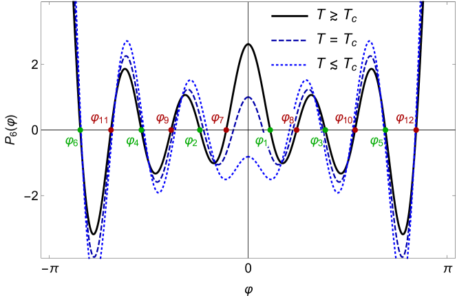
Figure 2: Characteristic polynomial $P_{M}(\varphi)$, equation (49), for $M=6$ above, at, and below $T_{\mathrm{c}}$. The eigenvalues are ordered as shown (see text).

Using the characteristic polynomial $P_{M}(\varphi)$ we can come back to the arrangement of the eigenvalues $\lambda$ of $\bm{\mathrm{\mathcal{T}}}_{\!\!2}$ and $\bm{\mathrm{\mathcal{T}}}_{\!\!}$. It turns out that it is beneficial to sort the $2M$ eigenvalues $\lambda$ of $\bm{\mathrm{\mathcal{T}}}_{\!\!2}$ by the value of $\varphi$, first selecting the zeroes of $P_{M}(\varphi)$ with negative slope ordered by $|\varphi|$ (green points in figure 2), and then selecting the zeroes of $P_{M}(\varphi)$ with positive slope ordered by $|\varphi|$ (red points in figure 2). Slightly below $T_{\mathrm{c}}$ the two zeroes $\varphi_{1}$ and $\varphi_{M+1}$ are zero and become complex below Hucht16b . However, the corresponding values $\lambda_{1}$ and $\lambda_{M+1}$ are always real and define the correct order.

The arrangement is compatible with (32) and leads to the following identities: from equation (47), we derive the identities

$$\sin\frac{\varphi}{2} =-\frac{\sqrt{z-t\lambda}\sqrt{t-z\lambda}}{2\sqrt{tz\lambda}\sqrt{t_{-}z_{-}}},$$ (50a)

$$\cos\frac{\varphi}{2} =\frac{\sqrt{\lambda-tz}\sqrt{1-tz\lambda}}{2\sqrt{tz\lambda}\sqrt{t_{-}z_{-}}},$$ (50b)

$$\tan\frac{\varphi}{2} =-\frac{\sqrt{z-t\lambda}\sqrt{t-z\lambda}}{\sqrt{\lambda-tz}\sqrt{1-tz\lambda}}$$ (50c)

and, using the characteristic polynomial (49),

$$\sin\frac{M\varphi}{2} =\pm\frac{\sqrt{z-t\lambda}\sqrt{1-tz\lambda}}{2\sqrt{tz\lambda}\sqrt{t_{-}\lambda_{-}}},$$ (51a)

$$\cos\frac{M\varphi}{2} =\pm\frac{\sqrt{t-z\lambda}\sqrt{\lambda-tz}}{2\sqrt{tz\lambda}\sqrt{t_{-}\lambda_{-}}},$$ (51b)

$$\tan\frac{M\varphi}{2} =\frac{\sqrt{z-t\lambda}\sqrt{1-tz\lambda}}{\sqrt{t-z\lambda}\sqrt{\lambda-tz}}$$ (51c)

as well as

$$\frac{\sin(M\varphi)}{\sin\varphi}=-\frac{z_{-}}{\lambda_{-}}.$$ (52)

These identities will be used in the following to simplify the eigenvectors of $\bm{\mathrm{\mathcal{T}}}$.

VII Eigenvectors of $\bm{\mathrm{\mathcal{T}}}_{\!\!}$

The common eigenvectors of $\bm{\mathrm{\mathcal{T}}}_{\!\!}$, $\bm{\mathrm{\mathcal{T}}}_{\!\!+}$ and $\bm{\mathrm{\mathcal{T}}}_{\!\!-}$ can be calculated from the recursion matrix (48), too, and read

$$(\bm{\mathrm{x}})_{\lambda,n}=(\vec{x}_{\lambda})_{n} \propto\langle\begin{array}[]{cc}1,&0\end{array}|\,\bm{\mathrm{Q}}^{n}\,|\begin{array}[]{cc}1,&t^{*}/z^{*}\end{array}\rangle$$ (55)

$$\propto\frac{\sin([n+1]\varphi)}{(1-t)(1+z)}-\frac{\sin(n\varphi)}{(1+t)(1-z)},$$ (56)

with $n=0,\ldots,M-1$. After proper normalization and an index change from $n$ to $m=-M+1,-M+3,\cdots,M-1$, running over the odd integers between $-M$ and $M$, the matrix elements of $\bm{\mathrm{x}}$ are

$$(\bm{\mathrm{x}})_{\lambda,m}=\frac{\sqrt{4tz}\,t_{-}z_{-}\lambda_{-}}{\sqrt{M\lambda_{-}^{2}+z_{+}\lambda_{+}-t_{+}}\,\sqrt{\lambda_{+}-1}}\left[\frac{\sin([M+1+m]\frac{\varphi}{2})}{(1-t)(1+z)}-\frac{\sin([M-1+m]\frac{\varphi}{2})}{(1+t)(1-z)}\right].$$ (57)

The block-diagonal transfer matrix (36) enables us to reduce the problem of calculating the partition function from $2M\times 2M$ matrices to $M\times M$ matrices, and to factorize the involved determinants. This will be demonstrated in the following chapter.

VIII Partition function factorization

Using the eigensystem defined above and the block diagonal form (36), we can write the partition function (29a) as

$$\mathcal{Z} =\det\langle\bm{\mathrm{S}}^{+}\;\bm{\mathrm{S}}^{-}|\begin{bmatrix}\bm{\mathrm{\mathcal{T}}}_{\!\!}^{L}&0\\ 0&\bm{\mathrm{\mathcal{T}}}_{\!\!}^{-L}\end{bmatrix}|\bm{\mathrm{S}}^{+}\;\bm{\mathrm{S}}^{-}\rangle$$ (58a)

$$=\det\big{(}\bm{\mathrm{S}}^{+}\bm{\mathrm{\mathcal{T}}}_{\!\!}^{L}\,\bm{\mathrm{S}}^{+}+\bm{\mathrm{S}}^{-}\bm{\mathrm{\mathcal{T}}}_{\!\!}^{-L}\,\bm{\mathrm{S}}^{-}\big{)},$$ (58b)

with $\bm{\mathrm{S}}^{\pm}\equiv\frac{1}{2}\left(\bm{\mathrm{1}}\pm\bm{\mathrm{S}}\right)$. At this point we define the $M\times M$ matrix

$$\bm{\mathrm{M}}\equiv\bm{\mathrm{x}}\big{(}\bm{\mathrm{\mathcal{T}}}_{\!\!}^{L/2}\,\bm{\mathrm{S}}^{+}+\bm{\mathrm{\mathcal{T}}}_{\!\!}^{-L/2}\,\bm{\mathrm{S}}^{-}\big{)},$$ (59)

which completes the square in (58b), as

$$\bar{\bm{\mathrm{M}}}\bm{\mathrm{M}} =\big{(}\bm{\mathrm{S}}^{+}\bm{\mathrm{\mathcal{T}}}_{\!\!}^{L/2}+\bm{\mathrm{S}}^{-}\bm{\mathrm{\mathcal{T}}}_{\!\!}^{-L/2}\,\big{)}\bar{\bm{\mathrm{x}}}\,\bm{\mathrm{x}}\big{(}\bm{\mathrm{\mathcal{T}}}_{\!\!}^{L/2}\,\bm{\mathrm{S}}^{+}+\bm{\mathrm{\mathcal{T}}}_{\!\!}^{-L/2}\,\bm{\mathrm{S}}^{-}\big{)}$$

$$=\bm{\mathrm{S}}^{+}\bm{\mathrm{\mathcal{T}}}_{\!\!}^{L}\,\bm{\mathrm{S}}^{+}+\bm{\mathrm{S}}^{+}\bm{\mathrm{S}}^{-}+\bm{\mathrm{S}}^{-}\bm{\mathrm{S}}^{+}+\bm{\mathrm{S}}^{-}\bm{\mathrm{\mathcal{T}}}_{\!\!}^{-L}\,\bm{\mathrm{S}}^{-}$$

$$=\bm{\mathrm{S}}^{+}\bm{\mathrm{\mathcal{T}}}_{\!\!}^{L}\,\bm{\mathrm{S}}^{+}+\bm{\mathrm{S}}^{-}\bm{\mathrm{\mathcal{T}}}_{\!\!}^{-L}\,\bm{\mathrm{S}}^{-}$$ (60)

and the mixed terms in the expansion vanish, $\bm{\mathrm{S}}^{+}\bm{\mathrm{S}}^{-}=\bm{\mathrm{S}}^{-}\bm{\mathrm{S}}^{+}=\frac{1}{4}\left(\bm{\mathrm{1}}-\bm{\mathrm{S}}^{2}\right)=\bm{\mathrm{0}}$. With $\bm{\mathrm{x}}\bm{\mathrm{\mathcal{T}}}_{\!\!}^{\pm L/2}=\bm{\mathrm{\Lambda}}^{\pm L/2}\bm{\mathrm{x}}$ from (34) the matrix elements of $\bm{\mathrm{M}}$ are

$$(\bm{\mathrm{M}})_{\lambda,m}=\tfrac{1}{2}(\lambda^{L/2}+\lambda^{-L/2}\,)(\bm{\mathrm{x}})_{\lambda,m}+\tfrac{1}{2}(\lambda^{L/2}-\lambda^{-L/2}\,)(\bm{\mathrm{x}})_{\lambda,-m},$$ (61)

and the partition function (58) becomes

$$\mathcal{Z}=\det\left(\bar{\bm{\mathrm{M}}}\bm{\mathrm{M}}\right)={\textstyle\det^{2}\bm{\mathrm{M}}},$$ (62)

i. e. $Z\propto\det\bm{\mathrm{M}}$.

We now insert the definition of $\bm{\mathrm{x}}$ from (57) and pull out common $m$-independent factors, primarily the normalization constants, which we can move into a diagonal matrix $\bm{\mathrm{D}}$ according to

$$\bar{\bm{\mathrm{M}}}\bm{\mathrm{M}}\equiv\bar{\bm{\mathrm{W}}}\bm{\mathrm{D}}\bm{\mathrm{W}}.$$ (63)

We first choose the decomposition

$$(\bm{\mathrm{W}}^{\ddagger})_{\lambda,m} \equiv\frac{1}{2}\sum_{\pm}(\lambda^{L/2}\pm\lambda^{-L/2})\left(\frac{\sin([M+1\pm m]\frac{\varphi}{2})}{(1-t)(1+z)}-\frac{\sin([M-1\pm m]\frac{\varphi}{2})}{(1+t)(1-z)}\right),$$ (64a)

$$(\bm{\mathrm{D}}^{\ddagger})_{\lambda,\lambda} \equiv\frac{8tz\lambda\,(t_{-}z_{-}\lambda_{-})^{2}}{(M\lambda_{-}^{2}+z_{+}\lambda_{+}-t_{+})\,(1-\lambda)^{2}},$$ (64b)

and sort $(\bm{\mathrm{W}}^{\ddagger})_{\lambda,m}$ by terms in $\lambda^{\pm L/2}$ to get, after some trigonometry,

$$(\bm{\mathrm{W}}^{\ddagger})_{\lambda,m}=\frac{\sin\varphi}{4tt_{-}zz_{-}} \left[\lambda^{L/2}\left((t-z)\frac{\sin\frac{M\varphi}{2}}{\sin\frac{\varphi}{2}}-(tz-1)\frac{\cos\frac{M\varphi}{2}}{\cos\frac{\varphi}{2}}\right)\cos\frac{m\varphi}{2}\right.$$

$${}+\left.\lambda^{-L/2}\left((t-z)\frac{\cos\frac{M\varphi}{2}}{\sin\frac{\varphi}{2}}+(tz-1)\frac{\sin\frac{M\varphi}{2}}{\cos\frac{\varphi}{2}}\right)\sin\frac{m\varphi}{2}\right].$$ (65)

Pulling out some factors and rearranging terms we get

$$(\bm{\mathrm{W}}^{\ddagger})_{\lambda,m}=\frac{\sin\varphi\cos\frac{M\varphi}{2}}{4tt_{-}zz_{-}} \left[\lambda^{L/2}\left((t-z)\frac{\tan\frac{M\varphi}{2}}{\tan\frac{\varphi}{2}}-(tz-1)\right)\frac{\cos\frac{m\varphi}{2}}{\cos\frac{\varphi}{2}}+{}\right.$$

$${}+\left.\lambda^{-L/2}\left((t-z)+(tz-1)\frac{\tan\frac{M\varphi}{2}}{\cot\frac{\varphi}{2}}\right)\frac{\sin\frac{m\varphi}{2}}{\sin\frac{\varphi}{2}}\right].$$ (66)

Further simplifications occur if we use the identities from (50) and (51), especially

$$\frac{\tan\frac{M\varphi}{2}}{\cot\frac{\varphi}{2}}=\frac{z-t\lambda}{tz-\lambda},\qquad\frac{\tan\frac{M\varphi}{2}}{\tan\frac{\varphi}{2}}=\frac{tz\lambda-1}{t-z\lambda}.$$ (67)

Shifting again $m$-independent factors from $\bm{\mathrm{W}}^{\ddagger}$ to $\bm{\mathrm{D}}^{\ddagger}$, the result can be simplified to

$$(\bm{\mathrm{W}}^{\dagger})_{\lambda,m} \equiv\frac{1}{\sqrt{t_{-}z_{-}}}\left[\lambda^{L/2}(tz-\lambda)\frac{\cos\frac{m\varphi}{2}}{\cos\frac{\varphi}{2}}-\lambda^{-L/2}(tz^{-1}-\lambda)\frac{\sin\frac{m\varphi}{2}}{\sin\frac{\varphi}{2}}\right]$$ (68a)

$$(\bm{\mathrm{D}})_{\lambda,\lambda} \equiv\frac{\lambda_{-}}{2z_{-}}\frac{(t_{+}z_{+}-\lambda_{+})^{2}-t_{-}^{2}z_{-}^{2}}{M\lambda_{-}^{2}+z_{+}\lambda_{+}-t_{+}}\,\frac{1}{(tz-\lambda)(tz^{-1}-\lambda)},$$ (68b)

and equation (62) becomes

$$\mathcal{Z}={\det}^{2}\bm{\mathrm{W}}^{\dagger}\;\prod_{\lambda}(\bm{\mathrm{D}})_{\lambda\lambda}.$$ (69)

The remaining challenge is the calculation of $\det\bm{\mathrm{W}}^{\dagger}$, which will be further simplified in the following.

IX The Vandermonde determinant

We now utilize the observation that the matrix $\bm{\mathrm{W}}^{\dagger}$ is a Vandermonde matrix, and that its determinant is invariant under basis transformations between complete polynomial bases. Hence we can transform $\bm{\mathrm{W}}^{\dagger}$ from the trigonometric basis to the simpler power basis. We identify the leading term in both $\cos\frac{m\varphi}{2}/\cos\frac{\varphi}{2}$ and $\sin\frac{m\varphi}{2}/\sin\frac{\varphi}{2}$ to be

$$\frac{\cos\frac{m\varphi}{2}}{\cos\frac{\varphi}{2}}\simeq\left(2\cos\frac{\varphi}{2}\right)^{|m|-1},\qquad\frac{\sin\frac{m\varphi}{2}}{\sin\frac{\varphi}{2}}\simeq\frac{m}{|m|}\left(2\cos\frac{\varphi}{2}\right)^{|m|-1}$$ (70)

and rewrite the result using (50b), as $2n\equiv|m|-1$ is an even integer, to

$$\left(2\cos\frac{\varphi}{2}\right)^{2n}=\left[\frac{(\lambda-tz)(1-tz\lambda)}{tz\lambda t_{-}z_{-}}\right]^{n}\simeq\left(\frac{-2}{t_{-}z_{-}}\right)^{n}\lambda_{+}^{n}.$$ (71)

The determinant becomes

$$\det\bm{\mathrm{W}}^{\dagger}=\left(\frac{2}{t_{-}z_{-}}\right)^{M^{2}/2}\det\bm{\mathrm{W}}$$ (72)

with

$$\bm{\mathrm{W}}=\left(\begin{array}[]{cccc|cccc}g_{1}c_{1}^{M/2-1}&\cdots&g_{1}c_{1}&g_{1}&f_{1}&f_{1}c_{1}&\cdots&f_{1}c_{1}^{M/2-1}\\ g_{2}c_{2}^{M/2-1}&\cdots&g_{2}c_{2}&g_{2}&f_{2}&f_{2}c_{2}&\cdots&f_{2}c_{2}^{M/2-1}\\ \vdots&&\vdots&\vdots&\vdots&\vdots&&\vdots\\ g_{M}c_{M}^{M/2-1}&\cdots&g_{M}c_{M}&g_{M}&f_{M}&f_{M}c_{M}&\cdots&f_{M}c_{M}^{M/2-1}\end{array}\right),$$ (73)

where we introduced the abbreviations

$$c_{\mu}\equiv\lambda_{\mu,+},\quad g_{\mu}\equiv-\lambda_{\mu}^{L/2}(tz-\lambda_{\mu}),\quad f_{\mu}\equiv\lambda_{\mu}^{-L/2}(tz^{-1}-\lambda_{\mu}).$$ (74)

Using a block Laplace expansion along the vertical line in (73), the determinant of $\bm{\mathrm{W}}$ can be written as alternating sum over all possible $\nicefrac{{M}}{{2}}\times\nicefrac{{M}}{{2}}$ $g$-minors $\det\bm{\mathrm{W}}_{\vphantom{\bar{\mathbf{s}}}\mathbf{s},\{1,\ldots,\nicefrac{{M}}{{2}}\}}$, times the corresponding $f$-minors $\det\bm{\mathrm{W}}_{\bar{\mathbf{s}},\{\nicefrac{{M}}{{2}}+1,\ldots,M\}}$,

$$\det\bm{\mathrm{W}}=\pm\sum_{\vphantom{\bar{\mathbf{s}}}\mathbf{s}}\operatorname{sign}(\vphantom{\bar{\mathbf{s}}}\mathbf{s},\bar{\mathbf{s}})\underbrace{\prod_{\mu\in\vphantom{\bar{\mathbf{s}}}\mathbf{s}}g_{\mu}\>\prod_{\mu<\nu\in\vphantom{\bar{\mathbf{s}}}\mathbf{s}}\negmedspace(c_{\mu}-c_{\nu})}_{\det\bm{\mathrm{W}}_{\vphantom{\bar{\mathbf{s}}}\mathbf{s},\{1,\ldots,\nicefrac{{M}}{{2}}\}}}\>\underbrace{\prod_{\mu\in\bar{\mathbf{s}}}f_{\mu}\>\prod_{\mu<\nu\in\bar{\mathbf{s}}}\negmedspace(c_{\mu}-c_{\nu})}_{\det\bm{\mathrm{W}}_{\bar{\mathbf{s}},\{\nicefrac{{M}}{{2}}+1,\ldots,M\}}},$$ (75)

where $\vphantom{\bar{\mathbf{s}}}\mathbf{s}$ denotes one of the $\binom{M}{M/2}$ possible subsets of $\nicefrac{{M}}{{2}}$ choices of the index set $\{1,\ldots,M\}$, and $\bar{\mathbf{s}}$ its complement. Both minors are simple Vandermonde determinants, and the irrelevant overall sign depends on the ordering within the sets.

In the following, we further reduce the matrix size from $M\times M$ to $\nicefrac{{M}}{{2}}\times\nicefrac{{M}}{{2}}$ by Vandermonde-type row elimination. While for simple Vandermonde determinants this procedure leads a complete factorization, in our case we can only eliminate $\nicefrac{{M}}{{2}}$ rows, which we nevertheless can choose arbitrary. We now denote the chosen set of eliminated rows and its complement by $\vphantom{\bar{\mathbf{s}}}\mathbf{s}$ and $\bar{\mathbf{s}}$ and find ($\bm{\mathrm{A}}_{\vphantom{\bar{\mathbf{s}}}\mathbf{s}}\equiv\bm{\mathrm{A}}_{\vphantom{\bar{\mathbf{s}}}\mathbf{s},\vphantom{\bar{\mathbf{s}}}\mathbf{s}}$)

$$\det\bm{\mathrm{W}}=\pm d_{\vphantom{\bar{\mathbf{s}}}\mathbf{s},\bar{\mathbf{s}}}\det\left(\bm{\mathrm{G}}_{\vphantom{\bar{\mathbf{s}}}\mathbf{s}}\bm{\mathrm{T}}_{\vphantom{\bar{\mathbf{s}}}\mathbf{s},\bar{\mathbf{s}}}\bm{\mathrm{F}}_{\bar{\mathbf{s}}}-\bm{\mathrm{F}}_{\vphantom{\bar{\mathbf{s}}}\mathbf{s}}\bm{\mathrm{T}}_{\vphantom{\bar{\mathbf{s}}}\mathbf{s},\bar{\mathbf{s}}}\bm{\mathrm{G}}_{\bar{\mathbf{s}}}\right),$$ (76)

with the $M\times M$ matrices

$$(\bm{\mathrm{G}})_{\mu\mu}\equiv g_{\mu},\quad(\bm{\mathrm{F}})_{\mu\mu}\equiv f_{\mu},\quad(\bm{\mathrm{T}})_{\mu\nu}\equiv\frac{1}{c_{\mu}-c_{\nu}},$$ (77a)

(we can set $$(\bm{\mathrm{T}})_{\mu\mu}\equiv 0 \mu\neq\nu$$, as ), and with the double product

$$d_{\vphantom{\bar{\mathbf{s}}}\mathbf{s},\bar{\mathbf{s}}}\equiv\prod_{\mu\in\vphantom{\bar{\mathbf{s}}}\mathbf{s}}\prod_{\nu\in\bar{\mathbf{s}}}(c_{\mu}-c_{\nu}).$$ (77b)

As $\bm{\mathrm{T}}_{\vphantom{\bar{\mathbf{s}}}\mathbf{s},\bar{\mathbf{s}}}$ is a Cauchy matrix, both $\bm{\mathrm{G}}_{\vphantom{\bar{\mathbf{s}}}\mathbf{s}}\bm{\mathrm{T}}_{\vphantom{\bar{\mathbf{s}}}\mathbf{s},\bar{\mathbf{s}}}\bm{\mathrm{F}}_{\bar{\mathbf{s}}}$ and $\bm{\mathrm{F}}_{\vphantom{\bar{\mathbf{s}}}\mathbf{s}}\bm{\mathrm{T}}_{\vphantom{\bar{\mathbf{s}}}\mathbf{s},\bar{\mathbf{s}}}\bm{\mathrm{G}}_{\bar{\mathbf{s}}}$ are Cauchy-like matrices. An example with $M=6$ and $\vphantom{\bar{\mathbf{s}}}\mathbf{s}=\{1,3,5\}$, such that $\bar{\mathbf{s}}=\{2,4,6\}$, reads

$$\bm{\mathrm{G}}_{\vphantom{\bar{\mathbf{s}}}\mathbf{s}}=\left(\begin{array}[]{ccc}g_{1}\\ &g_{3}\\ &&g_{5}\end{array}\right),\quad\bm{\mathrm{F}}_{\bar{\mathbf{s}}}=\left(\begin{array}[]{ccc}f_{2}\\ &f_{4}\\ &&f_{6}\end{array}\right),\quad\bm{\mathrm{T}}_{\vphantom{\bar{\mathbf{s}}}\mathbf{s},\bar{\mathbf{s}}}=\left(\begin{array}[]{ccc}\frac{1}{c_{1}-c_{2}}&\frac{1}{c_{1}-c_{4}}&\frac{1}{c_{1}-c_{6}}\\ \frac{1}{c_{3}-c_{2}}&\frac{1}{c_{3}-c_{4}}&\frac{1}{c_{3}-c_{6}}\\ \frac{1}{c_{5}-c_{2}}&\frac{1}{c_{5}-c_{4}}&\frac{1}{c_{5}-c_{6}}\end{array}\right).$$ (78)

The choice of $\vphantom{\bar{\mathbf{s}}}\mathbf{s}$ has influence on the magnitude of the two terms in (76) and has a physical interpretation: if we choose $\vphantom{\bar{\mathbf{s}}}\mathbf{s}=\mathbf{o}\equiv\{1,3,\ldots,M-1\}$ odd integers, both $\bm{\mathrm{G}}_{\vphantom{\bar{\mathbf{s}}}\mathbf{s}}$ and $\bm{\mathrm{F}}_{\bar{\mathbf{s}}}$ contain only dominant (for large $L$) eigenvalues $\lambda_{\mu}>1$, while the subdominant ones $\lambda_{\mu}<1$ enter $\bm{\mathrm{G}}_{\bar{\mathbf{s}}}$ and $\bm{\mathrm{F}}_{\vphantom{\bar{\mathbf{s}}}\mathbf{s}}$. Therefore, the term $\bm{\mathrm{G}}_{\vphantom{\bar{\mathbf{s}}}\mathbf{s}}\bm{\mathrm{T}}_{\vphantom{\bar{\mathbf{s}}}\mathbf{s},\bar{\mathbf{s}}}\bm{\mathrm{F}}_{\bar{\mathbf{s}}}$ in (76) gives the leading contribution for large $L$, and the second one $\bm{\mathrm{F}}_{\vphantom{\bar{\mathbf{s}}}\mathbf{s}}\bm{\mathrm{T}}_{\vphantom{\bar{\mathbf{s}}}\mathbf{s},\bar{\mathbf{s}}}\bm{\mathrm{G}}_{\bar{\mathbf{s}}}$ the finite-$L$ corrections. The oscillating behavior

$$\operatorname{sign}\log\lambda_{\mu}=\operatorname{sign}\gamma_{\mu}=\operatorname{sign}\varphi_{\mu}=(-1)^{\mu-1},\quad\mu=1,\ldots,M,$$ (79)

is dictated by the ordering of the zeroes of $P_{M}(\varphi)$, equation (49), as described above.

Consequently, we factor out the leading first term of the determinant in (76),

$$\det\bm{\mathrm{W}}=\pm d_{\vphantom{\bar{\mathbf{s}}}\mathbf{s},\bar{\mathbf{s}}}\det\big{(}\bm{\mathrm{G}}_{\vphantom{\bar{\mathbf{s}}}\mathbf{s}}\bm{\mathrm{T}}_{\vphantom{\bar{\mathbf{s}}}\mathbf{s},\bar{\mathbf{s}}}\bm{\mathrm{F}}_{\bar{\mathbf{s}}}\big{)}\det\big{(}\bm{\mathrm{1}}-\bm{\mathrm{F}}_{\bar{\mathbf{s}}}^{-1}\bm{\mathrm{T}}_{\vphantom{\bar{\mathbf{s}}}\mathbf{s},\bar{\mathbf{s}}}^{-1}\bm{\mathrm{G}}_{\vphantom{\bar{\mathbf{s}}}\mathbf{s}}^{-1}\bm{\mathrm{F}}_{\vphantom{\bar{\mathbf{s}}}\mathbf{s}}\bm{\mathrm{T}}_{\vphantom{\bar{\mathbf{s}}}\mathbf{s},\bar{\mathbf{s}}}\bm{\mathrm{G}}_{\bar{\mathbf{s}}}\big{)},$$ (80)

and express the inverse $\bm{\mathrm{T}}_{\vphantom{\bar{\mathbf{s}}}\mathbf{s},\bar{\mathbf{s}}}^{-1}$ through the diagonal matrix

$$(\bm{\mathrm{P}})_{\mu\mu}\equiv p_{\mu}\equiv\prod_{\nu=1}^{M}{\vphantom{\prod}}^{\prime}(c_{\mu}-c_{\nu})^{-\sigma_{\mu}\sigma_{\nu}},$$ (81)

which fulfills

$$\bm{\mathrm{P}}_{\bar{\mathbf{s}}}\bm{\mathrm{T}}_{\bar{\mathbf{s}},\vphantom{\bar{\mathbf{s}}}\mathbf{s}}\bm{\mathrm{P}}_{\vphantom{\bar{\mathbf{s}}}\mathbf{s}}\bm{\mathrm{T}}_{\vphantom{\bar{\mathbf{s}}}\mathbf{s},\bar{\mathbf{s}}}=\bm{\mathrm{1}}.$$ (82)

Here, $\prod^{\prime}$ denotes the regularized product, with zero and infinite factors removed, and we have defined the parity of $\mu$

$$\sigma_{\mu}\equiv\left\{\begin{array}[]{cc}+1&\quad\text{if }\mu\in\vphantom{\bar{\mathbf{s}}}\mathbf{s}\hphantom{.}\\ -1&\quad\text{if }\mu\in\bar{\mathbf{s}}.\end{array}\right.$$ (83)

We now introduce the diagonal matrix

$$(\bm{\mathrm{V}})_{\mu\mu}\equiv v_{\mu}\equiv-p_{\mu}\lambda_{\mu}^{L}\left(\frac{g_{\mu}}{f_{\mu}}\right)^{\sigma_{\mu}}=p_{\mu}\frac{tz^{-\sigma_{\mu}}-\lambda_{\mu}}{tz^{\sigma_{\mu}}-\lambda_{\mu}}$$ (84)

and define, with $\bm{\mathrm{\Lambda}}$ from (33), for the specific set of dominant odd indices $\mathbf{o}$ as well as the complementary set of even indices $\mathbf{e}\equiv\bar{\mathbf{o}}$ the residual matrix

$$\bm{\mathrm{Y}}\equiv-\bm{\mathrm{\Lambda}}_{\mathbf{e}}^{L}\bm{\mathrm{V}}_{\mathbf{e}}\bm{\mathrm{T}}_{\mathbf{e},\mathbf{o}}\bm{\mathrm{\Lambda}}_{\mathbf{o}}^{-L}\bm{\mathrm{V}}_{\mathbf{o}}\bm{\mathrm{T}}_{\mathbf{o},\mathbf{e}}$$ (85)

to find

$$\det\bm{\mathrm{W}}=\pm d_{\mathbf{o},\mathbf{e}}\det\bm{\mathrm{T}}_{\mathbf{o},\mathbf{e}}\det\bm{\mathrm{G}}_{\mathbf{o}}\det\bm{\mathrm{F}}_{\mathbf{e}}\det(\bm{\mathrm{1}}+\bm{\mathrm{Y}}).$$ (86)

Remember that the matrices with one index are diagonal. The determinant of the Cauchy matrix $\bm{\mathrm{T}}_{\vphantom{\bar{\mathbf{s}}}\mathbf{s},\bar{\mathbf{s}}}$ reads

$$\det\bm{\mathrm{T}}_{\vphantom{\bar{\mathbf{s}}}\mathbf{s},\bar{\mathbf{s}}}=\pm\frac{q_{\vphantom{\bar{\mathbf{s}}}\mathbf{s}}q_{\bar{\mathbf{s}}}}{d_{\vphantom{\bar{\mathbf{s}}}\mathbf{s},\bar{\mathbf{s}}}},$$ (87)

with

$$q_{\vphantom{\bar{\mathbf{s}}}\mathbf{s}}\equiv\prod_{\mu<\nu\in\vphantom{\bar{\mathbf{s}}}\mathbf{s}}\negmedspace(c_{\mu}-c_{\nu}),$$ (88)

leading to the final form

$$\det\bm{\mathrm{W}}=|q_{\mathbf{o}}q_{\mathbf{e}}|\det\bm{\mathrm{G}}_{\mathbf{o}}\det\bm{\mathrm{F}}_{\mathbf{e}}\det(\bm{\mathrm{1}}+\bm{\mathrm{Y}}).$$ (89)

X Resulting partition function

Introducing the strip residual partition function

$$Z_{\mathrm{strip}}^{\mathrm{res}}\equiv\det(\bm{\mathrm{1}}+\bm{\mathrm{Y}})$$ (90)

for the remaining determinant, and inserting explicit values for $\det\bm{\mathrm{G}}_{\mathbf{o}}$, $\det\bm{\mathrm{F}}_{\mathbf{e}}$ and $\det\bm{\mathrm{D}}$, we arrive at the final result

$$Z=\Bigg{[}C_{3}\,d_{\mathbf{o},\mathbf{e}}^{2}\,\prod_{\mu=1}^{M}\frac{(t_{+}z_{+}-\lambda_{\mu,+})^{2}-t_{-}^{2}z_{-}^{2}}{M\lambda_{\mu,-}^{2}+z_{+}\lambda_{\mu,+}-t_{+}}\,\frac{\sigma_{\mu}\lambda_{\mu,-}}{v_{\mu}}\,\lambda_{\mu}^{\sigma_{\mu}L}\Bigg{]}^{1/2}\>Z_{\mathrm{strip}}^{\mathrm{res}}$$ (91a)

for the partition function, with parity $$\sigma_{\mu}=(-1)^{\mu-1} d_{\mathbf{o},\mathbf{e}}$$, from (77b), and the constant

$$C_{3}\equiv z^{M}\left(\frac{2}{z_{-}}\right)^{LM}\left(\frac{2}{t_{-}z_{-}}\right)^{M^{2}/2}.$$ (91b)

We can discuss two limiting cases with respect to the aspect ratio $\rho$: by definition, the matrix $\bm{\mathrm{Y}}$ only contains subdominant finite-$L$ contributions, and therefore $\lim_{\rho\to\infty}\bm{\mathrm{Y}}=\bm{\mathrm{0}}$ and $\lim_{\rho\to\infty}Z_{\mathrm{strip}}^{\mathrm{res}}=1$. On the other hand, the limit $\rho\to 0$ can also be discussed. As $L$ is a real number in (85), we can let $L\to 0$ and find a Cauchy-type matrix very similar to one describing the spontaneous magnetization of the superintegrable chiral Potts model, as discussed by Baxter Baxter10a . The resulting determinant can be factorized and reads

$$\lim_{\rho\to 0}Z_{\mathrm{strip}}^{\mathrm{res}}=\pm\frac{(2tz_{-})^{M/2}{\displaystyle\prod_{\mu\in\mathbf{o}}\prod_{\nu\in\mathbf{e}}(\lambda_{\mu}-\lambda_{\nu})}}{{\displaystyle\prod_{\mu=1}^{M}(tz^{\sigma_{\mu}}-\lambda_{\mu})\prod_{\mu<\nu\in\mathbf{o}}(1-\lambda_{\mu}\lambda_{\nu})\prod_{\mu<\nu\in\mathbf{e}}(1-\lambda_{\mu}\lambda_{\nu})}}.$$ (92)

To summarize, we find closed product representations for both limit cases $L/M\to\infty$ and $M/L\to\infty$ with finite $M$. The general case $0<\rho<\infty$, however, involves the nontrivial determinant (90).

The oscillating order of the eigenvalues introduced in Chapter V was a prerequisite for the simple block diagonalization of the block transfer matrix $\bm{\mathrm{\mathcal{T}}}_{\!\!2}$, equation (36), and the subsequent factorization of $Z$. However, now we observe that this oscillation is reversed by the sets $\mathbf{o}$ and $\mathbf{e}$ of odd and even indices, used in the definition of the residual matrix $\bm{\mathrm{Y}}$. Therefore, we rewrite the results (85) and (91a) in terms of the simpler non-oscillating dominant eigenvalues $\hat{\lambda}_{\mu}$. Using the parity $\sigma_{\mu}=(-1)^{\mu-1}$, we define

$$\hat{\lambda}_{\mu}\equiv\lambda_{\mu}^{\sigma_{\mu}}>1,\quad\hat{\gamma}_{\mu}\equiv\sigma_{\mu}\gamma_{\mu}=|\gamma_{\mu}|>0,\quad\hat{\varphi}_{\mu}\equiv\sigma_{\mu}\varphi_{\mu}\stackrel{{\scriptstyle\mu>1}}{{=}}|\varphi_{\mu}|>0,\quad\mu=1,\ldots,M,$$ (93)

implying $\hat{\lambda}_{\mu,+}=\lambda_{\mu,+}=\hat{c}_{\mu}=c_{\mu}$ and $\hat{\lambda}_{\mu,-}=\sigma_{\mu}\lambda_{\mu,-}=|\lambda_{\mu,-}|$, to get

$$\hat{v}_{\mu} =v_{\mu}=p_{\mu}\frac{tz^{-\sigma_{\mu}}-\hat{\lambda}_{\mu}^{\sigma_{\mu}}}{tz^{\sigma_{\mu}}-\hat{\lambda}_{\mu}^{\sigma_{\mu}}},$$ (94a)

$$\hat{\bm{\mathrm{Y}}} =\bm{\mathrm{Y}}=-\hat{\bm{\mathrm{\Lambda}}}_{\mathbf{e}}^{-L}\bm{\mathrm{V}}_{\mathbf{e}}\bm{\mathrm{T}}_{\mathbf{e},\mathbf{o}}\hat{\bm{\mathrm{\Lambda}}}_{\mathbf{o}}^{-L}\bm{\mathrm{V}}_{\mathbf{o}}\bm{\mathrm{T}}_{\mathbf{o},\mathbf{e}},$$ (94b)

leading to the partition function (91a) in terms of $$\hat{\lambda}_{\mu}$$,

$$Z=\Bigg{[}C_{3}\,d_{\mathbf{o},\mathbf{e}}^{2}\,\prod_{\mu=1}^{M}\frac{(t_{+}z_{+}-\hat{\lambda}_{\mu,+})^{2}-t_{-}^{2}z_{-}^{2}}{M\hat{\lambda}_{\mu,-}^{2}+z_{+}\hat{\lambda}_{\mu,+}-t_{+}}\,\frac{\hat{\lambda}_{\mu,-}}{v_{\mu}}\,\hat{\lambda}_{\mu}^{L}\Bigg{]}^{1/2}\det(\bm{\mathrm{1}}+\bm{\mathrm{Y}}).$$ (94c)

This is the final result of our analysis for arbitrary temperature $T$ and finite system size $L$ and $M$. We factorized the partition function up to the factor $Z_{\mathrm{strip}}^{\mathrm{res}}$, equation (90), where the residual matrix $\bm{\mathrm{Y}}$ contains all information about the finite aspect ratio $\rho$ and will be analyzed in detail in Hucht16b . The first term in (94c) is the infinite strip contribution, which has been analyzed in great detail by Baxter recently Baxter16 .

XI Free energy contributions

In this chapter we give a decomposition of the reduced free energy (in units of $k_{\mathrm{B}}T$)

$$F(T;L,M)=-\log Z$$ (95)

appropriate for our geometry and method. We first recall that

$$F(T;L,M)=F_{\infty}(T;L,M)+F_{\infty}^{\mathrm{res}}(T;L,M),$$ (96)

with infinite volume contribution $F_{\infty}$, that for our geometry has the form

$$F_{\infty}(T;L,M)\equiv LMf_{\mathrm{b}}(T)+Lf_{\mathrm{s}}^{\leftrightarrow}(T)+Mf_{\mathrm{s}}^{\updownarrow}(T)+f_{\mathrm{c}}(T),$$ (97)

and can be viewed as a regularization term in the limit $L,M\to\infty$. The bulk free energy per spin $f_{\mathrm{b}}(T)$, surface free energies per surface spin pair $f_{\mathrm{s}}^{\delta}(T)$, and corner free energy $f_{\mathrm{c}}(T)$ are defined in the thermodynamic limit $L,M\to\infty$ and do not depend on $L,M$. However, the residual free energy $F_{\infty}^{\mathrm{res}}$, denoted $O(\mathrm{e}^{-\gamma L},\mathrm{e}^{-\gamma M})$ in equation (1.1) of Baxter16 , gives rise to important finite-size effects, most prominently the Casimir amplitude and the critical Casimir force Hucht16b .

In the limit $L\to\infty$ with fixed $M$, the strip residual partition function $Z_{\mathrm{strip}}^{\mathrm{res}}\to 1$, as shown in the last chapter. Consequently, we denote the infinite strip contribution

$$Z_{\mathrm{strip}}\equiv Z/Z_{\mathrm{strip}}^{\mathrm{res}}$$ (98)

and get a free energy decomposition slightly different from (96), namely

$$F(T;L,M)=F_{\mathrm{strip}}(T;L,M)+F_{\mathrm{strip}}^{\mathrm{res}}(T;L,M),$$ (99)

where we can identify the strip residual free energy

$$F_{\mathrm{strip}}^{\mathrm{res}}\equiv-\log\det(\bm{\mathrm{1}}+\bm{\mathrm{Y}})$$ (100)

as the $L$-dependent term in the difference between the residual free energy $F_{\infty}^{\mathrm{res}}$ of the finite rectangular system and the leading divergent term $\mathcal{O}(L)$ in the limit $L\to\infty$ HuchtGruenebergSchmidt11 ,

$$F_{\mathrm{strip}}^{\mathrm{res}}(T;L,M)=F_{\infty}^{\mathrm{res}}(T;L,M)-L\lim_{L\to\infty}L^{-1}F_{\infty}^{\mathrm{res}}(T;L,M)-F_{\mathrm{s,c}}^{\mathrm{res}}(T;M).$$ (101)

Note that the last term $F_{\mathrm{s,c}}^{\mathrm{res}}(T;M)$ drops out in the $L$-derivative below, for details we refer to Hucht16b . In this notation, Vernier & Jacobsen VernierJacobsen12 conjectured a product representation of the infinite volume contribution $Z_{\infty}\equiv\mathrm{e}^{-F_{\infty}}$ that trivially depends on the system size $L$ and $M$, see also appendix A, while Baxter derived a product formula for the infinite strip contribution $Z_{\mathrm{strip}}$ at finite strip width $M$, and then performed the limit $M\to\infty$ Baxter16 . Both results applied only to the ordered phase below $T_{\mathrm{c}}$.

Finally we turn to the critical Casimir force. The reduced Casimir force per area $M$ in $L$ direction reads

$$\mathcal{F}(T;L,M)\equiv-\frac{1}{M}\frac{\partial}{\partial L}F_{\infty}^{\mathrm{res}}(T;L,M)$$ (102)

and can be decomposed into two parts to find, in analogy to (101), the differential contribution

$$\mathcal{F}_{\mathrm{strip}}(T;L,M) \equiv-\frac{1}{M}\frac{\partial}{\partial L}F_{\mathrm{strip}}^{\mathrm{res}}(T;L,M)$$ (103a)

$$=\mathcal{F}(T;L,M)+\frac{1}{M}\lim_{L\to\infty}L^{-1}F_{\infty}^{\mathrm{res}}(T;L,M).$$ (103b)

This contribution is therefore directly related to the remaining determinant (90). For details on the involved universal amplitudes and finite-size scaling functions the reader again is referred to Hucht16b .

XII Effective spin model

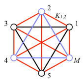
Figure 3: Effective spin model for $M=6$. The two sublattices of odd and even spins are shown as black and light blue circles. The black and light blue interactions between spins of same parity are ferromagnetic, while the red couplings are antiferromagnetic. Note that the spatial arrangement of the spins is arbitrary, as all couplings $K_{\mu\nu}$ are different.

In this last chapter we present an exact mapping of the residual determinant $Z_{\mathrm{strip}}^{\mathrm{res}}$, equation (90), onto an effective spin model with $M$ spins and long-range pair interactions. This model might be a starting point for further investigations of the residual determinant. The mapping is motivated by the observation that the determinant expansion of (90) is of the form (here we set $L=0$ for simplicity)

$$Z_{\mathrm{strip}}^{\mathrm{res}}=1+\underbrace{\sum_{\mu\in\mathbf{o}}\sum_{\nu\in\mathbf{e}}\frac{v_{\mu}v_{\nu}}{(c_{\mu}-c_{\nu})^{2}}}_{1^{\mathrm{st}}\,\mathrm{order}}+\underbrace{\sum_{\mu\neq\mu^{\prime}\in\mathbf{o}}\sum_{\nu\neq\nu^{\prime}\in\mathbf{e}}\frac{v_{\mu}v_{\mu^{\prime}}v_{\nu}v_{\nu^{\prime}}(c_{\mu}-c_{\mu^{\prime}})^{2}(c_{\nu}-c_{\nu^{\prime}})^{2}}{(c_{\mu}-c_{\nu})^{2}(c_{\mu}-c_{\nu^{\prime}})^{2}(c_{\mu^{\prime}}-c_{\nu})^{2}(c_{\mu^{\prime}}-c_{\nu^{\prime}})^{2}}}_{2^{\mathrm{nd}}\,\mathrm{order}}+\ldots$$ (104)

and consists of $\binom{M}{M/2}$ positive terms. Hence we identify these terms with the Boltzmann factors $\mathrm{e}^{-\mathcal{H}_{\mathrm{eff}}}$ of the $\binom{M}{M/2}$ possible spin configurations of $M$ spins $s_{\mu}\in\{0,1\}$ under the constraint

$$\sum_{\mu\in\mathbf{o}}s_{\mu}=\sum_{\nu\in\mathbf{e}}s_{\nu}\quad\Leftrightarrow\quad\sum_{\mu=1}^{M}\sigma_{\mu}s_{\mu}=0.$$ (105)

We interpret $\mathbf{o}$ and $\mathbf{e}$ as two sublattices, discriminated by the parity $\sigma_{\mu}$, equation (83), see figure 3. The effective spin model then has the Hamiltonian

$$\mathcal{H}_{\mathrm{eff}}=-\sum_{\mu<\nu=1}^{M}K_{\mu\nu}s_{\mu}s_{\nu}+L\sum_{\mu=1}^{M}\hat{\gamma}_{\mu}s_{\mu}+b\Big{[}\sum_{\mu=1}^{M}\sigma_{\mu}s_{\mu}\Big{]}^{2},$$ (106)

with interaction constants

$$K_{\mu\nu}=-\sigma_{\mu}\sigma_{\nu}\log\frac{v_{\mu}v_{\nu}}{(c_{\mu}-c_{\nu})^{2}},$$ (107)

while the positive $\hat{\gamma}_{\mu}$ from (93) play the role of magnetic moments in a homogeneous magnetic field of strength $-L$. Both the couplings $K_{\mu\nu}$ as well as the magnetic moments $\hat{\gamma}_{\mu}$ depend on the temperature of the underlying Ising model, and the limit $b\to\infty$ enforces the constraint (105). As $(c_{\mu}-c_{\nu})^{2}>v_{\mu}v_{\nu}$ for all $\mu,\nu$, the couplings $K_{\mu\nu}$ are ferromagnetic for spins within the same set and antiferromagnetic between different sets, as shown in figure 3. For $L>0$, the external magnetic field is antiparallel to the spins and favors states with small magnetization. Consequently, for magnetic field $L\to\infty$ all spins are forced to have $s_{\mu}=0$.

With these definitions, the residual determinant (90) is equal to the partition function of the Hamiltonian (106) in the limit $b\to\infty$,

$$Z_{\mathrm{strip}}^{\mathrm{res}}=Z_{\mathrm{eff}}\equiv\operatorname{Tr}\mathrm{e}^{-\mathcal{H}_{\mathrm{eff}}},$$ (108)

where the trace effectively runs over the $\binom{M}{M/2}$ spin states compatible with condition (105), and (104) coincides with the expansion of $Z_{\mathrm{eff}}$ around the high-field limit $L\to\infty$. In this expansion we start with $s_{\mu}=0$ ($Z_{\mathrm{eff}}=1$) and flip one spin in both sublattices to get the first order term. For two reversed spins in both subsystems we find the second order term, and so on.

On the other hand, the zero-field case $L=0$ is described by (92), which means that we have found a closed form solution for the partition function (106) at vanishing applied field.

The Casimir quantities translate into the effective model as follows: the strip Casimir potential, or strip residual free energy, (100) is simply the free energy of the effective model (106),

$$F_{\mathrm{strip}}^{\mathrm{res}}(T;L,M)=-\log Z_{\mathrm{strip}}^{\mathrm{res}}=-\log\operatorname{Tr}\mathrm{e}^{-\mathcal{H}_{\mathrm{eff}}}.$$ (109)

By the definition (103a), the differential Casimir force per surface area $M$ is given by

$$\mathcal{F}_{\mathrm{strip}}(T;L,M) =-\frac{1}{M}\frac{\partial}{\partial L}F_{\mathrm{strip}}^{\mathrm{res}}(T;L,M)$$

$$=\frac{1}{M}\frac{\partial}{\partial L}\log\operatorname{Tr}\mathrm{e}^{-\mathcal{H}_{\mathrm{eff}}}$$

$$=-\frac{1}{M}\Big{\langle}\sum_{\mu=1}^{M}\hat{\gamma}_{\mu}s_{\mu}\Big{\rangle}_{\mathrm{eff}}\equiv-m_{\mathrm{eff}}(L),$$ (110)

and is therefore identical to minus the field dependent magnetization per spin of the effective model in an antiparallel magnetic field of strength $L$.

From this mapping, one could conclude that the residual determinant $Z_{\mathrm{strip}}^{\mathrm{res}}$ cannot be factorized into a product for arbitrary $L$, as this would imply an exact solution of a spin system with long range frustrated interactions in a magnetic field. However, the couplings (107) are products of symmetric functions of the $c_{\mu}$, which might be utilized to find a factorization. In the finite-size scaling limit $L,M\to\infty$, $T\to T_{\mathrm{c}}$, at fixed temperature scaling variable $x\propto(T/T_{\mathrm{c}}-1)L$ and aspect ratio $\rho$, such a factorization indeed exists at least at the critical point $T_{\mathrm{c}}$. In this limit, the residual determinant (90) can be written in terms of the Dedekind eta function Hucht16b , confirming a result from conformal field theory KlebanVassileva91 .

XIII Conclusions

We have calculated the partition function of the two-dimensional anisotropic square lattice Ising model on a $L\times M$ rectangle with open boundary conditions. The final expression (94) involves $M$ eigenvalues $\hat{\lambda}_{\mu}$ of a $M\times M$ transfer matrix, represented as zeroes of its characteristic polynomial (49). The remaining residual part (90) is reduced to the determinant of a $\nicefrac{{M}}{{2}}\times\nicefrac{{M}}{{2}}$ matrix, for which we could not find a closed product representation (see also FredMathoverflow16 ).

An analogous calculation, with similar result (94), can be done for arbitrary coupling distributions $z_{\ell<L,m}=z_{m}$, $t_{\ell,m}=t_{m}$, as long as the involved transfer matrix $\bm{\mathrm{\mathcal{T}}}_{\!\!2}$, equation (27), is independent of $\ell$. The characteristic polynomial, eigenvalues and eigenvectors of $\bm{\mathrm{\mathcal{T}}}_{\!\!}$, equation (34), will however be more complicated. On the other hand, we can return to cylinder geometry with periodic or antiperiodic boundary conditions, $z_{\ell<L,m}=z$, $t_{\ell,m<M}=t$, $t_{\ell,M}=t^{\pm 1}$, in which case the characteristic polynomial (49) simply becomes $P_{M}^{(\mathrm{pbc})}(\varphi)=\cos\!\left(\frac{M\varphi}{2}\right)$ or $P_{M}^{(\mathrm{apbc})}(\varphi)=\sin\!\left(\frac{M\varphi}{2}\right)$ independent of temperature, which greatly simplifies the calculations.

The intermediate result (25) gives the exact partition function of the Ising model with arbitrary couplings $K_{\ell,m}^{\leftrightarrow}$ and $K_{\ell,m}^{\updownarrow}$ on the cylinder in terms of a product of very simple $2\times 2$ block transfer matrices with $M\times M$ blocks. This representation can be used to, e. g., investigate diluted systems, or to exactly determine the critical Casimir potential and force between extended particles on the lattice, as introduced in HobrechtHucht14 ; HobrechtHucht15a . Due to the reduction to $2M\times 2M$ matrices, numerically exact calculations are possible for large systems up to $M\approx 1000$ and arbitrary $L$ on actual personal computers. However, depending on the actual coupling configuration it might be necessary to use extended numerical precision.

Finally, we presented an exact mapping of the residual part $Z_{\mathrm{strip}}^{\mathrm{res}}$ of the partition function onto an effective spin system with long-range frustrated interactions in an external magnetic field of strength $L$. This model might serve as starting point for further investigations.

The finite-size scaling limit of the considered model, as well as results for the Casimir potential and Casimir force scaling functions, will be published in the second part of this work Hucht16b .

Appendix A Product formulas for free energy contributions

In this appendix we will give, without derivation, the product formulas for the singular parts of the free energies $f_{\mathrm{b}}$, $f_{\mathrm{s}}$ and $f_{\mathrm{c}}$ above and below $T_{\mathrm{c}}$ for the isotropic Ising model, where $K=K^{\leftrightarrow}=K^{\updownarrow}$ and $z=t^{*}$. The calculation is done similar to VernierJacobsen12 : using the finite lattice method Enting78 we generate the high- and low-temperature series expansion of the free energies up to some finite order and rewrite the series in terms of the natural variable $q$ BaxterSykesWatts75 using the inverse Euler transform MathWorld-EulerTransform . Interestingly, both the finite lattice method and the inverse Euler transform are based on the Möbius inversion formula from elementary number theory Hardy79 . The resulting infinite product in $q$ has a periodic structure

$$\prod_{k=1}^{\infty}(1-q^{k})^{c_{0,k}+c_{1,k}k},$$ (111)

i. e., the coefficients $c_{0,k}$ and $c_{1,k}$ are oscillating sequences, with period $p\in\{4,8,16\}$, which can be identified. These sequences are then conjectured to continue to $k\to\infty$. First we recall the results of Vernier & Jacobsen VernierJacobsen12 obtained for temperatures below $T_{\mathrm{c}}$.

Infinite products like (111) can be written in many different ways. For the sake of clarity we first introduce a simple notation for such periodic products: we define the function

$$\operatorname{\Pi}(\bm{\mathrm{C}}|q)\equiv\prod_{k=1}^{\infty}(1-q^{k})^{c_{k}},$$ (112)

where the $(m+1)\times p$ coefficient matrix $\bm{\mathrm{C}}$ defines the $m^{\mathrm{th}}$-order polynomials

$$c_{k}=\sum_{j=0}^{m}\bm{\mathrm{C}}_{j,k\,\mathrm{mod}\,p}\,k^{j}.$$ (113)

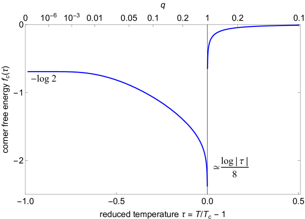
Figure 4: Corner free energy $f_{\mathrm{c}}$ vs. reduced temperature of the two-dimensional Ising model. The corresponding values of the natural variable $q$ are shown at the upper frame.

With this definition we first rewrite the results of Vernier & Jacobsen: the natural low temperature variable $q$ fulfills (VernierJacobsen12, , equation (48))

$$t^{<} =\sqrt{q}\,\operatorname{\Pi}\big{(}\begin{array}[]{cccccccc}0&1&0&-1&0&-1&0&1\end{array}|\,q\big{)}$$ (115)

$$=\sqrt{q}\frac{(q;q^{8})_{\infty}(q^{7};q^{8})_{\infty}}{(q^{3};q^{8})_{\infty}(q^{5};q^{8})_{\infty}}=\sqrt{q}\frac{(1-q^{1})(1-q^{7})(1-q^{9})(1-q^{15})\cdots}{(1-q^{3})(1-q^{5})(1-q^{11})(1-q^{13})\cdots},$$

where $t^{<}=\mathrm{e}^{-2K^{<}}$, and $(a;q)_{\infty}$ denotes the $q$-Pochhammer symbol. Then, the singular bulk, surface and corner free energies become (VernierJacobsen12, , equation (49))

$$e^{-f_{\mathrm{b,sing}}^{<}} =\frac{1}{\sqrt{q}}\operatorname{\Pi}\left(\left.\begin{array}[]{cccccccc}0&0&-1&0&2&0&-1&0\\ 0&-1&0&1&0&-1&0&1\end{array}\right|q\right),$$ (116c)

$$e^{-f_{\mathrm{s,sing}}^{<}} =\frac{1}{2}\operatorname{\Pi}\left(\left.\begin{array}[]{cccccccc}0&\frac{3}{4}&-1&-\frac{3}{4}&2&-\frac{3}{4}&-1&\frac{3}{4}\\ 0&\frac{1}{4}&0&\frac{1}{4}&0&-\frac{1}{4}&0&-\frac{1}{4}\end{array}\right|q\right)\operatorname{\Pi}\left(\left.\begin{array}[]{cccccccc}0&-\frac{1}{2}&0&\frac{1}{2}&0&\frac{1}{2}&0&-\frac{1}{2}\\ 0&-\frac{1}{2}&0&-\frac{1}{2}&0&\frac{1}{2}&0&\frac{1}{2}\end{array}\right|\sqrt{q}\right),$$ (116h)

$$e^{-f_{\mathrm{c}}^{<}} =2\operatorname{\Pi}\left(\left.\begin{array}[]{cccccccc}0&-2&3&-2&-1&-2&3&-2\\ 0&-2&\frac{1}{2}&2&0&-2&-\frac{1}{2}&2\end{array}\right|q\right),$$ (116k)

where the regular part of $f_{\mathrm{c}}$ is zero, while $f_{\mathrm{b,reg}}=-\log[2(1+z^{2})/(1-z^{2})]$ and $f_{\mathrm{s,reg}}=-\frac{1}{4}\log(1-z^{2})$. Doing the same analysis in the paramagnetic phase we first identify the high temperature variable $z^{>}=\tanh K^{>}$ by duality BaxterSykesWatts75 , such that

$$z^{>}=\sqrt{q}\,\operatorname{\Pi}\big{(}\begin{array}[]{cccccccc}0&1&0&-1&0&-1&0&1\end{array}|\,q\big{)}$$ (117)

has the same product representation as (115). Then we find the infinite products

$$e^{-f_{\mathrm{b,sing}}^{>}} =\operatorname{\Pi}\left(\left.\begin{array}[]{cccccccc}0&2&-4&2&0&2&-4&2\\ 0&-1&0&1&0&-1&0&1\end{array}\right|q\right)=\operatorname{\Pi}\left(\left.\begin{array}[]{cccc}0&2&-4&2\\ 0&-1&0&1\end{array}\right|q\right),$$ (118e)

$$e^{-f_{\mathrm{s,sing}}^{>}} =\operatorname{\Pi}\left(\left.\begin{array}[]{cccccccc}0&\frac{1}{4}&1&-\frac{1}{4}&-2&-\frac{1}{4}&1&\frac{1}{4}\\ 0&-\frac{1}{4}&0&-\frac{1}{4}&0&\frac{1}{4}&0&\frac{1}{4}\end{array}\right|q\right),$$ (118h)

$$e^{-f_{\mathrm{c}}^{>}} =\operatorname{\Pi}\left(\left.\begin{array}[]{cccccccc}0&0&0&0&-3&0&0&0\\ 0&0&-\frac{1}{2}&0&0&0&\frac{1}{2}&0\end{array}\right|q\right)=\operatorname{\Pi}\left(\left.\begin{array}[]{cccc}0&0&-3&0\\ 0&-1&0&1\end{array}\right|q^{2}\right)$$ (118m)

$$=\prod_{k=0}^{\infty}\frac{1}{(1-q^{2(4k+2)})^{3}}\frac{(1-q^{2(4k+3)})^{4k+3}}{(1-q^{2(4k+1)})^{4k+1}}.$$ (118n)

Note that the period of all three products above $T_{\mathrm{c}}$ is half of the period below $T_{\mathrm{c}}$ ($e^{-f_{\mathrm{s,sing}}^{<}}$ can be written as a single product in $\sqrt{q}$, with period 16). The second product in $e^{-f_{\mathrm{s,sing}}^{<}}$ is interpreted as the additional contribution from the surface tension. The corner free energy $f_{\mathrm{c}}^{>}$ can be written as a function of $q^{2}$, because $c_{k}\neq 0$ only for even numbers $k$. Finally, we show the corner free energy $f_{\mathrm{c}}$ in figure 4. For $T\to 0$, $f_{\mathrm{c}}\to-\log 2$, while for $T\to T_{\mathrm{c}}$ we find a logarithmic divergence from both sides, with different amplitudes. A detailed discussion of the critical region will be presented in Hucht16b .

References

- [1] E. Ising. Beitrag zur Theorie des Ferromagnetismus. Z. Phys., 31:253, 1925.
- [2] L. Onsager. Crystal statistics. I. A two-dimensional model with an order-disorder transition. Phys. Rev., 65:117, 1944.
- [3] B. M. McCoy and T. T. Wu. The Two-Dimensional Ising Model. Harvard University Press, Cambridge, 1973.
- [4] R. J. Baxter. Exactly Solved Models in Statistical Mechanics. Academic Press, London, 1982.
- [5] M. E. Fisher and P.-G. de Gennes. Phénomènes aux parois dans un mélange binaire critique. C. R. Acad. Sci. Paris, Ser. B, 287:207, 1978.
- [6] H. B. G. Casimir. On the attraction between two perfectly conducting plates. Proc. K. Ned. Akad. Wet., 51:793, 1948.
- [7] R. Evans and J. Stecki. Solvation force in two-dimensional Ising strips. Phys. Rev. B, 49:8842–8851, Apr 1994.
- [8] Helen Au-Yang and Michael E. Fisher. Wall effects in critical systems: Scaling in Ising model strips. Phys. Rev. B, 21:3956, 1980.
- [9] J. G. Brankov, D. M. Dantchev, and N. S. Tonchev. Theory of Critical Phenomena in Finite-Size Systems – Scaling and Quantum Effects. World Scientific, Singapore, 2000.
- [10] A. E. Ferdinand and M. E. Fisher. Bounded and inhomogeneous Ising models. I. Specific-heat anomaly of a finite lattice. Phys. Rev., 185:832, 1969.
- [11] Wentao T. Lu and F. Y. Wu. Ising model on nonorientable surfaces: Exact solution for the Möbius strip and the Klein bottle. Phys. Rev. E, 63:026107, 2001.
- [12] P Kleban and I Vassileva. Free energy of rectangular domains at criticality. J. Phys. A: Math. Gen., 24:3407, 1991.
- [13] Alfred Hucht, Daniel Grüneberg, and Felix M. Schmidt. Aspect-ratio dependence of thermodynamic Casimir forces. Phys. Rev. E, 83:051101, Mar 2011.
- [14] Hendrik Hobrecht and Alfred Hucht. Critical Casimir force scaling functions of the two-dimensional Ising model at finite aspect ratios. J. Stat. Mech.: Theory Exp., 2017:024002, Feb 2017. arXiv:1611.05622.
- [15] Alfred Hucht. The square lattice Ising model on the rectangle II: finite-size scaling limit. J. Phys. A: Math. Theor., 50(26):265205, 2017. arXiv:1701.08722.
- [16] Eric Vernier and Jesper Lykke Jacobsen. Corner free energies and boundary effects for Ising, Potts and fully-packed loop models on the square and triangular lattices. J. Phys. A: Math. Theor., 45:045003, 2012. arXiv:1110.2158.
- [17] R. J. Baxter. The bulk, surface and corner free energies of the square lattice Ising model. J. Phys. A: Math. Theor., 50(1):014001, 2017. arXiv:1606.02029.
- [18] P. W. Kasteleyn. Dimer statistics and phase transitions. J. Math. Phys., 4:287, 1963.
- [19] Luca G. Molinari. Determinants of block tridiagonal matrices. Linear Algebra Appl., 429:2221, 2008. arXiv:0712.0681.
- [20] Michael E. Fisher. Statistical mechanics of dimers on a plane lattice. Phys. Rev., 124(6):1664, 1961.
- [21] R. J. Baxter. Spontaneous magnetization of the superintegrable chiral Potts model: calculation of the determinant . J. Phys. A: Math. Theor., 43(14):145002, 2010.
- [22] Fred Hucht. Determinant of a certain Vandermonde matrix, April 2016. http://mathoverflow.net/questions/236323/.
- [23] Hendrik Hobrecht and Alfred Hucht. Direct simulation of critical Casimir forces. EPL, 106(5):56005, Jun 2014. arXiv:1405.4088.
- [24] Hendrik Hobrecht and Alfred Hucht. Many-body critical Casimir interactions in colloidal suspensions. Phys. Rev. E, 92:042315, Oct 2015.
- [25] I. G. Enting. Generalised Möbius functions for rectangles on the square lattice. J. Phys. A: Math. Gen., 11(3):563, 1978.
- [26] R. J. Baxter, M. F. Sykes, and M. G. Watts. Magnetization of the three-spin triangular Ising model. J. Phys. A: Math. Gen., 8:245, 1975.
- [27] Eric W. Weisstein. Euler Transform. From MathWorld–A Wolfram Web Resource. http://mathworld.wolfram.com/EulerTransform.html.
- [28] G. H. Hardy and E. M. Wright. An Introduction to the Theory of Numbers. Oxford Univ. Press, Oxford, 5 edition, 1979.