Effects of long-range disorder and electronic interactions on the optical properties of graphene quantum dots

Abstract

We theoretically investigate the effects of long-range disorder and electron-electron interactions on the optical properties of hexagonal armchair graphene quantum dots consisting of up to 10806 atoms. The numerical calculations are performed using a combination of tight-binding, mean-field Hubbard and configuration interaction methods. Imperfections in the graphene quantum dots are modelled as a long-range random potential landscape, giving rise to electron-hole puddles. We show that, when the electron-hole puddles are present, tight-binding method gives a poor description of the low-energy absorption spectra compared to meanfield and configuration interaction calculation results. As the size of the graphene quantum dot is increased, the universal optical conductivity limit can be observed in the absorption spectrum. When disorder is present, calculated absorption spectrum approaches the experimental results for isolated monolayer of graphene sheet.

I Introduction

Graphene, single layer of carbon atoms arranged in a two-dimensional honeycomb latticewallace1947band ; novoselov2004electric , has attracted enormous research interest due to superior electronic electrical conductivitynovoselov2004electric ; novoselov2005two ; zhang2005experimental ; rycerz2007valley , mechanical strengthlee2008measurement ; dikin2007preparation ; mechanicthermal1 , thermal conductivitymechanicthermal1 and unique optical propertiesoptical1 ; optical2 . Moreover, the electronic and optical properties of graphene can be manipulated at the nanoscale in a desired way by controlling lateral size, shape, type of edge, doping level and the number of layers in graphene nanostructuresnanostructures1 ; nanostructures2 ; nanostructures3 ; nanostructures4 ; nanostructures5 ; nanoribbonedge5 . Among those various nanostructures of graphene, graphene quantum dots (GQDs)nanostructures6 ; GrapheneQuantumDotBook ; quantumdot1 ; quantumdot2 ; quantumdot3 ; quantumdot4 ; quantumdot4a ; quantumdot6 ; quantumdot7 ; magneticzigzag1 ; devrimexcitonic2 ; devrimmagnetic1 ; opticzigzag1 ; opticzigzag2 ; opticzigzag3 ; electronicoptic1 offer a possibility to simultaneously control the electronic, magnetic and optical functionalities in a single material.

GQDs are classified according to their edge character since the edges play an important role in determining electronic, optical and magnetic properties of GQDsquantumdot1 ; quantumdot2 ; quantumdot3 ; quantumdot4 ; quantumdot6 ; quantumdot7 ; quantumdot4a ; magneticzigzag1 ; devrimmagnetic1 ; devrimexcitonic2 . In particular, armchair and zigzag edges are the most stable edge structuresnanoribbonedge5 ; quantumdot6 ; quantumdot7 while GQDs with zigzag edges are found to exhibit unusual magneticquantumdot4a ; magneticzigzag1 ; devrimmagnetic1 and opticaldevrimexcitonic2 ; opticzigzag1 ; opticzigzag2 ; opticzigzag3 ; electronicoptic1 properties due to the presence of a degenerate band of states at the Fermi level. On the other hand, armchair edges do not lead to degenerate band of states at the Fermi level, hence, can be used as small model of bulk graphene which does not have edge statesarmchair1 .

Properties of graphene nanostructures fabricated and observed upon substratessubstrate1 ; substrate2 may become affected by imperfections due to the environment and become disordered. In particular, if the disorder has a long-range character, it can lead to charge localizations as electron-hole puddlespuddle1 ; puddle2 ; puddle3 ; puddle4 . For instance, magnetic properties of graphene nanoribbons are found to be strongly dependent of long-range impuritiesulasmenafdevrim . In addition, the role of electron-hole puddles on the formation of Landau levels in a graphene double quantum dot was investigated experimentally by K. L. Chiu et al.disorderpuddle1 .

On the other hand, a striking optical property of graphene is the universal optical conductivity (UOC) which can be identified as explicit manifestation of light and matter interactionUOC1 ; UOC2 ; opticconductance3 . The experimental observation of UOC for a graphene sheet seems to indicate that optical properties are robust against imperfections, although significant deviations from UOC at lower energies was observedopticconductance1 ; opticconductance2 . To our knowledge, a detailed theoretical investigation of combined effects of long-range disorder and electron-electron interactions on the optical properties of graphene quantum dots is still lacking.

In this work, we investigate theoretically electronic and optical properties of medium and large sized hexagonal armchair GQDs consisting of up to 10806 atoms to understand the role of long-ranged disorder on the optical properties. Our main contribution involves inclusion of electron-electron interactions within meanfield and many-body configuration interaction approaches. We show that the electron-electron interactions play a significant role in redistributing electron-hole puddles, thus strongly affecting the optical properties. We also investigate the large size limit of the GQDs as compared to optical properties of bulk grapheneopticconductance1 ; opticconductance2 ; opticconductance3 and show that UOC can be observed in GQDs with a diameter of 18 nm.

The paper is organized as follows. In Sec. II, we describe our model Hamiltonian including electron-electron interaction and random potential term, and the computational methods that we use in order to compute optical properties of hexagonal armchair GQDs. The computational results on the electronic and optical properties are presented in Sec. III. Finally, Section IV provides summary and conclusion.

II Method and Model

In the tight-binding (TB) approach, the one electron states of GQD can be written as a linear combination of $p_{z}$ orbitals on every carbon atom since the $s$, $p_{x}$ and $p_{y}$ orbitals are considered to be mainly responsible for mechanical stability of graphene. Then, within the meanfield extended Hubbard approach, Hamiltonian can be written as:

$$H_{MFH}= \sum_{ij\sigma}(t_{ij}c^{\dagger}_{i\sigma}c_{j\sigma}+h.c)$$

$$+U\sum_{i\sigma}(\operatorname{}\langle n_{i\sigma}\rangle-\frac{1}{2})n_{i\bar{\sigma}}+\sum_{ij\sigma}V_{ij}(\operatorname{}\langle n_{j}\rangle-1)n_{i\sigma}$$

$$+\sum_{i\sigma}V_{imp}(i)c^{\dagger}_{i\sigma}c_{i\sigma}$$ (1)

where the first term represents TB Hamiltonian and $t_{ij}$ are the hopping parameters given by $t_{nn}=-2.8$ eV for nearest neighbours and $t_{nnn}=-0.2$ eV for next nearest-neighbourshopping1 . The $c^{\dagger}_{i\sigma}$ and $c_{i\sigma}$ are creation and annihilation operators for an electron at the $i$th orbital having spin $\sigma$, respectively. Expectation value of electron densities are represented by $\operatorname{}\langle n_{i\sigma}\rangle$. The second and third terms represent onsite and long range Coulomb interaction, respectively. We take onsite interaction parameter as $U=16.522/\kappa$ eV and long-range interaction parameters $V_{ij}=8.64/\kappa$ and $V_{ij}=5.33/\kappa$ for the first and second nearest neighbours with effective dielectric constant $\kappa=6$dielectricconstant1 , respectively. Distant neighbor interaction is taken to be $1/d_{ij}\kappa$ and interaction matrix elements are obtained from numerical calculations by using Slater $\pi_{z}$ orbitals Slatermatrix1 . Last term corresponds to impurity potential $V_{imp}(i)$ account for substrate effects.

After diagonalizing the mean-field Hubbard (MFH) matrix self consistently by starting with TB orbitals, we obtain the Hubbard quasi-particle spectrum which has fully occupied valance band and completely empty conduction band. Next, in order to take into account two-body configuration interactions (CI), excitonic correlation effects of electron-hole, we solve the many-body Hamiltonian for a hole and an electron:

$$\begin{split}H_{eh}=&\sum\limits_{p^{\prime}\sigma}\epsilon_{p^{\prime}}b_{p^{\prime}\sigma}^{\dagger}b_{p^{\prime}\sigma}-\sum\limits_{p,\sigma}\epsilon_{p}h_{p\sigma}^{\dagger}h_{p\sigma}\\ &-\sum\limits_{\begin{subarray}{c}p^{\prime},q,r,s^{\prime}\\ \sigma,\sigma^{\prime}\end{subarray}}\left\{<rp^{\prime}\mid V\mid s^{\prime}q>\right.\\ &\left.-\left(1-\delta_{\sigma\sigma^{\prime}}\right)<rp^{\prime}\mid V\mid qs^{\prime}>\right\}b_{p^{\prime}\sigma}^{\dagger}h_{q\sigma^{\prime}}^{\dagger}h_{r\sigma^{\prime}}b_{s^{\prime}\sigma}\\ &+\sum\limits_{\begin{subarray}{c}p^{\prime},q,r,s^{\prime}\\ \sigma,\bar{\sigma}\end{subarray}}<rp^{\prime}\mid V\mid qs^{\prime}>b_{p^{\prime}\bar{\sigma}}^{\dagger}h_{q\sigma}^{\dagger}h_{r\bar{\sigma}}b_{s^{\prime}\sigma}\\ \end{split}$$ (2)

Here, the first two terms describe electron and hole quasi-particle energies obtained from the meanfield calculations, third term describes the electron-hole Coulomb attraction, and the fourth and fifth terms represent the electron-hole exchange interactions. Indices with prime denotes electron states and without prime denotes hole states. The two-body electron-hole scattering matrix elements are calculated from two-body on-site and long-range Coulomb matrix elements GrapheneQuantumDotBook .

In this work, we consider three different sizes of hexagonal armchair GQDs (see for example Fig. 1a) consisting of 1014, 5514 and 10806 atoms and having widths of 5 nm, 13 nm and 18 nm, respectively.

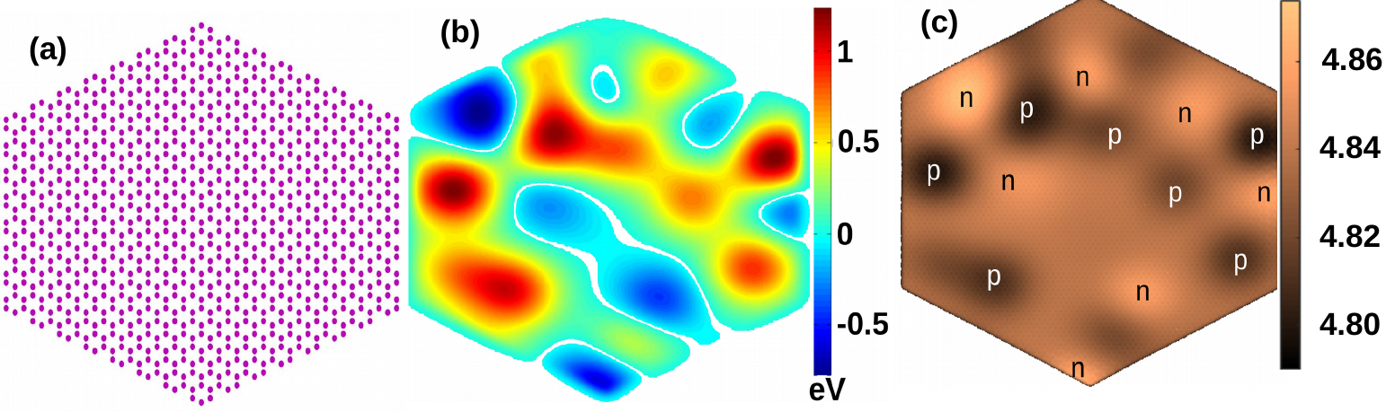
Figure 1: (Color online) (a) Lattice structure of hexagonal armchair edged GQD. (b) Impurity potential landscape. (c) Electron-hole puddle formation achieved by MFH model where local charge accumulation is indicated as n and p puddles.

In order to model the long-range disorder due to charge impurities caused by substrate effects, we use a superposition of Gaussian electrostatic potentials $V_{imp}$ which are determined randomly to have a smooth potential landscape (see Fig. 1b) on the GQD. Impurity potential is written as:

$$V_{imp}(r_{i})=\sum_{k}V_{k}\ exp\Big{[}{-\frac{(\vec{r}_{i}-\vec{R}_{k})^{2}}{2\sigma^{2}}}\Big{]}$$ (3)

where $V_{k}$ is chosen to be the potential peak value which is randomly generated between $-V_{max}<V_{k}<V_{max}$ values for an impurity at $R_{k}$, characterizing the strength of the disorder. For most of the calculations, we take $V_{max}=t_{nn}/3$ giving a medium disorder strength. However, the effect of strong ($V_{max}=t_{nn}$) and weak ($V_{max}=t_{nn}/5$) disorder is also investigated (see Fig. 5). The width of the potential, $\sigma$, is determined to be 10 times the lattice constant in order to simulate long-range lattice scatterers(puddle1, ). For 5 nm (1014 atoms), 13 nm (5514 atoms) and 18 (10806 atoms) nm wide GQDs, respectively 4, 20 and 40 source point of impurities are randomly created to have approximately similar source point densities (but different form of distribution of source points) for each GQD. Moreover, we considered 5 different randomly chosen potential configurations for each QD size. The main effect of long-range disorder on the electronic densities is the formation of electron-hole puddlespuddle1 ; ulasmenafdevrim , as seen from Fig. 1c, obtained by subtraction of the positive background charge from MFH electronic density. The effect of the electron-hole puddles on the optical properties will be investigated below using TB, MFH and CI approaches.

Interaction of GQD’s electrons with photons are evaluated within electric dipole approximation by the interaction Hamiltonian $H_{int}=\mathbf{E}\cdot\mathbf{r}$ where $\mathbf{E}$ is the photon’s electric field and $\mathbf{r}$ is the electron’s position. Hence, one can obtain absorption spectrum by using light-matter interaction which is described as:

$$A(\omega)=\sum_{f}\frac{4\pi^{2}\alpha E_{fi}{\mid<f\mid\mathbf{r}\mid i>\mid}^{2}\delta(\hbar\omega-E_{fi})}{Area}$$ (4)

where $\alpha$ is fine structure constant, $Area$ is area of the QD, $E_{fi}$ is the difference between initial and final energies, $<f\mid\mathbf{r}\mid i>$ denotes dipole matrix element, $\mid i>$ and $\mid f>$ denote initial and final occupied molecular orbitals , respectively, obtained by TB and MFH model.

On the other hand, we obtain absorption spectrum which includes many-body correlations as:

$$A(\omega)=\sum_{f}\frac{4\pi^{2}\alpha E_{fi}{\mid<f\mid\mathbf{P^{\dagger}}\mid gs>\mid}^{2}\delta(\hbar\omega-E_{fi})}{Area}$$ (5)

where $\alpha$ is fine structure constant, $Area$ is area of the QD, $E_{fi}$ is the difference between initial (ground state) and final energies of exciton, $\mathbf{P^{\dagger}}$ annihilates a photon and adds an exciton to the ground state of the GQD. The final excitonic state $\mid f>$ is obtained from CI calculations, and $\mid gs>$ is the ground state.

III Results

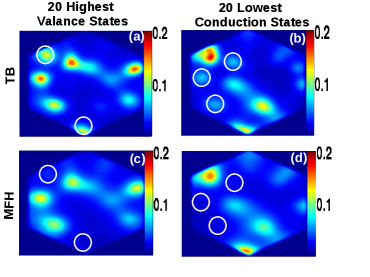
Figure 2: (Color online) Electronic density corresponding to the 20 highest valence states (left panels), and the 20 lowest conduction states (right panels), obtained from TB (upper panels) and MFH (lower panels) model of the structure 18 nm width size. Electron-electron interactions wash out abnormal localized states near Fermi level as indicated by white circles.

In Fig.2, we investigate electronic densities corresponding to 20 lowest conduction and 20 highest valence states obtained from TB and MFH calculations for the largest GQD structure that we studied, which has 10806 atoms giving a width of 18 nm (see corresponding potential landscape in Fig. 1b). We note that we repeated all the calculations for 5 different random potential landscape (for each QD size) and observed similar behaviors. In the TB results, in addition to valance states accumulated around peaks and conduction states around troughs (see Fig. 2a and 2b) as expected, we also observe abnormal valance states around troughs and conduction states around peaks (shown in circles, to be compared with Fig.1b). In fact, those abnormal states are an artifact of the TB method which is better suited for systems with homogeneous and neutral charge distributions. In our system, the charge density fluctuates strongly due to random disorder and the energy gap between valence and conduction states is not large enough to protect hole states from mixing with electron states. Thus, a mean-field correction to the TB method must be included. Indeed, when electron-electron interactions are included through MFH calculations, electronic density fluctuations are reduced in almost all area of the QD and the abnormal localized states are washed out (see Fig. 2c and 2d). Similar behavior was also observed in graphene nanoribbonsulasmenafdevrim . As we will see, the rearrangement of electron-hole puddles through electronic interactions has an important effect on optical properties.

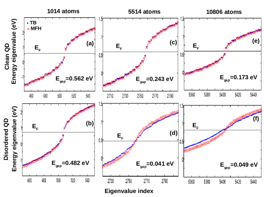
Figure 3: (Color online) Energy spectra for clean (upper panels) and disordered (lower panels) GQDs obtained by TB and MFH. Fermi energy level $E_{F}$ is determined to be in the mid-point between valance and conduction band.

Energy spectra of clean (upper panels) and disordered (lower panels) GQDs having width size of 5 nm (1014 atoms), 13 nm (5514 atoms) and 18 nm (10806 atoms) obtained by TB and MFH model are shown in Fig.3. For each case, the energy gap $E_{gap}$ between between lowest unoccupied conduction state and highest occupied valence state obtained from the MFH calculations is indicated as well. As expected, $E_{gap}$ decreases more rapidly as a function of size when impurities are present. More interestingly however, for larger size disordered GQDs the difference between TB and MFH spectra become pronounced indicating that when charge inhomogeneities (due to electron-puddle formation) are present it is important to include the effects of electronic interactions. Similar behavior was also observed for other random potential configurations that we have tested.

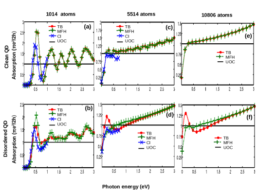
Figure 4: (Color online) Absorption Spectrum for clean (upper panels) and disordered (lower panels) GQDs obtained by TB, MFH and excitonic effect with CI model. UOC is indicated by black line. In clean GQDs, as the size of GQDs increase, a plateau develops near the UOC at low energies, before a sudden drop occurs due to finite size effects.

Figure 4 shows absorption spectra curves corresponding to the GQDs considered in Fig.3 for energies up to 3 eV. The absorption spectra are calculated using equations (4) and (5) with a Gaussian broadening (0.1 eV) of delta functions in order to obtain continuous curves, within TB (line doted curve, red color online), MFH (line plus signed curve, green color online) and CI (line cross signed curve, blue color online) approaches. The UOC is indicated by black line as a reference. For clean GQDs, there is no noticeable difference between the TB and MFH results, consistent with the results in Fig.3. We note that, as the system size increases, absorption curves approach the UOC value at low energies, until a sudden drop occurs due to finite size effects. For the CI calculations, 100 highest valence and 100 lowest conduction states were included to form a many-body basis set of 10000 excitonic states, to ensure convergence for energies up to 0.75 eV. As seen from Fig.4a and Fig.4b, the main effect of excitonic correlations is to red shift the absorption spectrumelectronicoptic1 followed by a slight decrease in the peak value. For GQDs larger than 13 nm (5514 atoms), it was not possible to calculate the CI absorption spectrum due to computational limits.

When disorder is present, we observe a dramatic difference between the TB and MFH results, shown in Fig.4b,d,f. This is mainly due to the redistribution of electron-hole puddles discussed in Fig.2. For the medium and large size GQDs without electronic interactions, in TB calculations, both electrons and hole puddles may be present at the same locations, giving rise to stronger electric dipole coupling, thus higher absorption values in average at lower energies. Note that the situation is different for the GQD with 1014 atoms, since the puddle formation is much less well defined as the size of the QD is reduced, and the specific form of the disorder landscape has a bigger role. For medium size GQD, however, a disorder peak reappears at low energies when excitonic correlations are taken into account. This is due to the fact that excitonic interactions rearranges the electron and hole distributions within the disorder troughs and peaks, as we discuss below in Fig.6. We note that the CI results obtained for the disordered GQD with 5514 atoms is consistent with the experimental results for graphene sheet optical1 ; opticconductance1 ; opticconductance2 .

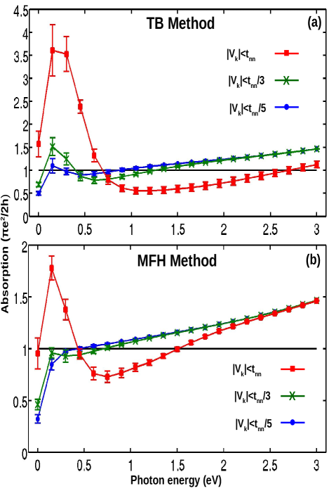
Figure 5: (Color online) Average absorption spectrum curves (each curve corresponds to average of 5 different configurations) for three different impurity potential peaks obtained by TB (upper panel) and MFH (lower panel) method with estimated error bars for the structure containing 10806 atoms. UOC is indicated by black line.

To see effects of various impurity potential strength on absorption spectrum obtained by TB and MFH methods (see Fig. 5a-b), we compare spectrum curves (each spectrum curve corresponds to average of five different samples shown with errorbars having width of twice the standard error) containing three different impurity potential strength peak values of $t_{nn}$ (line squared curve, red color online), $t_{nn}/3$ (line cross signed curve, green color online) and $t_{nn}/5$ (line doted curve, blue color online), for the largest QD structure. For the strong impurity potential strength ($|V_{k}|<t_{nn}$), both TB and MFH results deviate significantly from UOC line indicating that the system is in a strongly non-perturbative regime, and meanfield electron interactions are not sufficiently strong to wash out the impurity peak. However, for medium potential strength ($|V_{k}|<t_{nn}/3$) and small potential strength $|V_{k}|<t_{nn}/5$, the low energy absorption obtained from MFH remains always below the UOC line within our error bars.

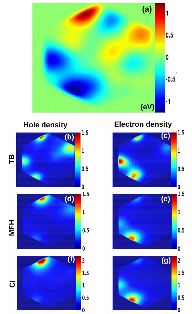
Figure 6: (Color online) (a) Impurity potential for the structure containing 5514 atoms. (b-g) show corresponding electron and hole densities weighted with absorption probabilities in the energy range between 0 eV and 0.3 eV obtained by TB, MFH and CI models, respectively.

In order to investigate the effect of excitonic correlations further, in Fig.6 we plot the electron and hole densities weighted with absorption probabilities in the energy range between 0 eV and 0.3 eV for the 5514 atom GQD, obtained from TB , MFH and CI calculations. As discussed earlier, mean-field interactions smooth the puddles so that excitonic hole states are now localized only on peaks, and the electron states are localized on troughs as seen in Fig.6d-e. On the other hand, the correlations have a less dramatic effect on the density distribution, but the electron states are now slightly more localized on a potential trough that is closer to the hole puddle (see Fig.6f-g). Indeed, the electron-hole attraction is favoured in the CI calculations minimizing the average distance between the electron and the hole, thus increasing the electric dipole strength and the absorption at lower energies.

IV Conclusions

In conclusion, we have investigated electronic and optic properties of three different sizes of clean and disordered hexagonal armchair-edged GQDs by applying tight-binding, mean-field Hubbard and configuration interaction models. Long-ranged disorder give rise to formation of electron-hole puddles, which are, however poorly described by the tight-binding model alone. Electronic interactions in the mean-field picture reorganize the electron-hole puddles, strongly affecting the dipole moments between the low-energy states in the electronic spectrum. Hence, inclusion of electronic interactions are found to be important in order to correctly describe the optical properties. As the system size is increased to 18 nm, absorption spectra obtained from configuration interaction method approach the experimental results leading to observation of universal optical conductivityopticconductance1 ; opticconductance2 .

References

- (1) P.R. Wallace, Physical Review 71, 622 (1947).
- (2) K.S. Novoselov, A.K. Geim, S.V. Morozov, D. Jiang, Y. Zhang, S.V. Dubonos, I.V. Grigorieva and A.A. Firsov, Science 306, 666 (2004).
- (3) K.S. Novoselov, A.K. Geim, S.V. Morozov, D. Jiang, M.I. Katsnelson, I.V. Grigorieva, S.V. Dubonos and A. A. Firsov, Nature 438, 197 (2005).
- (4) Yuanbo Zhang, Yan-Wen Tan, Horst L. Stormer and Philip Kim, Nature 438, 201 (2005).
- (5) A. Rycerz, J. Tworzydło and C.W.J. Beenakker, Nature 3, 172 (2007).
- (6) C. Lee, X. Wei, J.W. Kysar and J. Hone, Science 321, 385 (2008).
- (7) D.A. Dikin, S. Stankovich, E.J. Zimney, R.D. Piner, G.H.B. Dommett, G. Evmenenko, S.T. Nguyen and R.S. Ruoff, Nature 448, 457 (2007).
- (8) G. Xin, T. Yao, H. Sun, S.M Scott, D Shao, G. Wang and J. Lian, Science 349, 1083 (2015).
- (9) K.F. Mak, M.Y. Sfeir, Y. Wu, C.H. Lui, J.A. Misewich and T.F. Heinz, Physical Review Letters 101, 196405 (2008).
- (10) Y. Zhang, T.T. Tang, C. Girit, Z. Hao, M.C. Martin, A. Zettl, M.F. Crommie, Y.R. Shen and F. Wang, Nature 459, 820 (2009).
- (11) X. Li, X. Wang, L. Zhang, S. Lee and H. Dai, Science 319, 1229 (2008).
- (12) J. Cai, P. Ruffieux, R. Jaafar, M. Bieri, T. Braun, S. Blankenburg, M. Muoth, A.P. Seitsonen, M. Saleh, X. Feng, K. Müllen and R. Fasel, Nature 466, 470(2010).
- (13) M. Treier, C.A. Pignedoli, T. Laino, R. Rieger, K. Müllen, D. Passerone and R. Fasel, Nature Chemistry 3, 61 (2011).
- (14) M.L. Mueller, X. Yan, J.A. McGuire and L.S. Li, Nano Letters 10, 2679 (2010).
- (15) Y. Morita, S. Suzuki, K. Sato and T. Takui, Nature Chemistry 3, 197 (2011).
- (16) T. Wassmann, A. P. Seitsonen, A. M. Saitta, M. Lazzeri and F. Mauri, Physical Review Letters 101, 096402 (2008).
- (17) J. Shen , Y. Zhu, X. Yang and C Li, Chemical Communications 48, 3686 (2012).
- (18) A. D. Güçlü, P. Potasz, M. Korkusinski, and P. Hawrylak, Graphene Quantum Dots (NanoScience and Technology, Springer, Berlin, 2014).
- (19) K.A. Ritter and J.W. Lyding, Nature Materials 8, 235 (2009).
- (20) J. Peng, W. Gao, B.K. Gupta, Z. Liu, R.R. Aburto, L. Ge, L. Song, L.B. Alemany, X. Zhan, G. Gao, S. A. Vithayathil, B. A. Kaipparettu, A. A. Marti, T. Hayashi, J.J. Zhu and P. M. Ajayan, Nano Letters 12, 844 (2012).
- (21) B. Trauzettel, D.V. Bulaev, D. Loss and G. Burkard, Nature Physics 3, 192 (2007).
- (22) B.D. Gerardot, D. Brunner, P.A. Dalgarno, P. Öhberg, S. Seidl, M. Kroner, K. Karrai, N.G. Stoltz, P.M. Petroff and R.J. Warburton, Nature 451, 441 (2008).
- (23) M. Zarenia, A. Chaves, G.A. Farias and F.M. Peeters, Physical Review B 84, 245403 (2011).
- (24) O. Voznyy, A.D. Güçlü, P. Potasz and P. Hawrylak, Physical Review B 83, 165417 (2011).
- (25) P. Potasz, A.D. Güçlü, A. Wójs and P. Hawrylak, Physical Review B 85, 075431 (2012).
- (26) A.D. Güçlü, P. Potasz and P. Hawrylak, Physical Review B 84, 035425 (2011).
- (27) A.D. Güçlü, P. Potasz, O. Voznyy, M. Korkusinski and P. Hawrylak, Physical Review Letters 103, 246805 (2009).
- (28) A.D. Güçlü, P. Potasz and P. Hawrylak, Physical Review B 82, 155445 (2010).
- (29) T. Basak, H. Chakraborty and A. Shukla, Physical Review B 92, 205404 (2015).
- (30) C. Sun, F. Figge, I. Ozfidan, M. Korkusinski, X. Yan, L. Li, P. Hawrylak and J. A. McGuire, Nano Letters 15, 5472-5476 (2015).
- (31) Y. Li, H. Shu, S. Wang and J. Wang, The Journal of Physical Chemistry C, 119 4983-4989 (2015).
- (32) I. Ozfidan, A.D. Güçlü, M. Korkusinski and P. Hawrylak, Rapid Research Letters 9999, 1 (2015).
- (33) T. Yamamoto, T. Noguchi and K. Watanabe, Physical Review B 74, 121409 (2006).
- (34) L. Liao, Y.C. Lin, M. Bao, R. Cheng, J. Bai, Y. Liu, Y. Qu, K.L. Wang, Y. Huang and X. Duan, Nature 467, 305 (2010).
- (35) Y.M. Lin, C. Dimitrakopoulos, K.A. Jenkins, D.B. Farmer, H.Y. Chiu, A. Grill and Ph. Avouris, Science 327, 662 (2010).
- (36) Y. Zhang, V.W. Brar, C. Girit, A. Zettl and M.F. Crommie, Nature Physics 5, 722 (2009).
- (37) J. Martin, N. Akerman, G. Ulbricht, T. Lohmann, J.H. Smet, K.V Klitzing and A. Yacoby, Nature Physics 4, 144 (2008).
- (38) M. Gibertini, A. Tomadin, F. Guinea, M.I. Katsnelson and M. Polini, Physical Review B 85, 201405 (2012).
- (39) Y.W. Tan, Y. Zhang, K. Bolotin, Y. Zhao, S. Adam, E.H. Hwang, S. DasSarma, H.L. Stormer and P. Kim, Physical Review Letters 99, 246803 (2007).
- (40) H. U. Özdemir, A. Altıntaş and A. D. Güçlü, Physical Review B, 93 014415 (2016).
- (41) K. L. Chiu, M. R. Connolly, A. Cresti, J. P. Griffiths, G. A. C. Jones, and C. G. Smith, Physical Review B, 92 155408 (2015).
- (42) R. R. Nair, P. Blake, A. N. Grigorenko, K. S. Novoselov, T. J. Booth, T. Stauber, N. M. R. Peres and A. K. Geim, Science 320, 1308 (2008).
- (43) A. B. Kuzmenko, E. van Heumen, F. Carbone, and D. van der Marel, Physical Review Letters 100, 117401 (2008).
- (44) K.F. Mak, J. Shan and T.F. Heinz, Physical Review Letters 106, 046401 (2011).
- (45) C. Lee, J.Y. Kim, S. Bae, K.S. Kim, B.H. Hong and E.J. Choi, Applied Physics Letters 98, 071905 (2011).
- (46) S. Yuan, R. Roldan, H. DeRaedt and M. I. Katsnelson, Physical Review B 84, 195418 (2011).
- (47) S. Reich, J. Maultzsch, C. Thomsen and P. Ordejon, Physical Review B 66, 035412 (2002).
- (48) T. Ando, Journal of the Physical Society of Japan 75, 074716 (2006).
- (49) P. Potasz, A.D. Güçlü and P. Hawrylak, Phys. Rev. B 82, 075425 (2010).