Crawling and turning in a minimal reaction-diffusion cell motility model: coupling cell shape and biochemistry
Abstract
We study a minimal model of a crawling eukaryotic cell with a chemical polarity controlled by a reaction-diffusion mechanism describing Rho GTPase dynamics. The size, shape, and speed of the cell emerge from the combination of the chemical polarity, which controls the locations where actin polymerization occurs, and the physical properties of the cell, including its membrane tension. We find in our model both highly persistent trajectories, in which the cell crawls in a straight line, and turning trajectories, where the cell transitions from crawling in a line to crawling in a circle. We discuss the controlling variables for this turning instability, and argue that turning arises from a coupling between the reaction-diffusion mechanism and the shape of the cell. This emphasizes the surprising features that can arise from simple links between cell mechanics and biochemistry. Our results suggest that similar instabilities may be present in a broad class of biochemical descriptions of cell polarity.
I Introduction
Cell motility is a fundamental aspect of biology, crucial in processes ranging from morphogenesis to wound healing to cancer metastasis bray2001cell . Many aspects of cell motility have been extensively modeled, ranging from the biochemistry and physics of actin-polymerization-based protrusion mogilner2003force ; hu2010mechano , to the importance of cytoskeleton mechanics shao2012coupling ; rubinstein2009actin ; herant2010form to a wide variety of internal mechanisms for determining a cell’s orientation wolgemuth2011redundant ; maree2012cells ; jilkine2011comparison . Many of these aspects of the modeling of eukaryotic cell shape and motility have been reviewed in two recent papers holmes2012comparison ; ziebert2016computational .
In this paper, we will take a minimalistic approach, focusing on two main aspects of cell motility: the cell shape, as determined by a force balance at the surface of the cell, and the cell’s internal, chemical regulation of its direction, modeled by reaction-diffusion equations within the cell. This model can be characterized by a small number of unitless parameters – six physical and biochemical parameters, and a few others related to the numerical evaluation of the model. The relative simplicity of this model allows us to capture essential cell behaviors, but avoids the full parameter space of more detailed schemes.
Even with such a simple model, it is possible to create reasonable cell shapes, which can be regulated by both physical and chemical features. In addition, we show that both linear and circular crawling trajectories can be observed. We argue that the circular trajectories arise from a coupling between cell shape and the internal chemical polarity of the cell, and suggest that these effects should be visible in a broad variety of models for cell polarity. Our results may provide some insight into recent experiments linking cell turning events and cell speed gorelik2015arp2 .
II Model
We model the cell’s boundary as an interface with a tension applied to it, driven by actin polymerization at the front of the cell and myosin-based contraction at the cell rear. For simplicity, we neglect the membrane’s bending modulus; including it is straightforward shao2010computational , but we have found it does not qualitatively chage our results. The cell front and rear are characterized by the distribution of a membrane-bound Rho GTPase (a polarity protein), whose dynamics are given by a variant of the simple wave-pinning reaction-diffusion model established by Mori et al. mori2008wave . We assume that the motion of the cell membrane is overdamped, i.e. obeying a force balance . We assume that the actomyosin force is normally directed and proportional to ,
| (1) |
where and is the outward-pointing normal to the cell. Similar assumptions are used in shao2010computational ; wolgemuth2011redundant ; camley2014polarity . This corresponds to a cell pushing out at the front, where and contracting at the back, where ; is thus a measure of protrusiveness and a measure of contractility. We assume that the membrane has a tension (a line tension, since we are working in two dimensions), and thus exerts a force per unit length of
| (2) |
where is the local curvature of the membrane. We assume a fluid-like friction, proportional to the velocity of the cell boundary,
| (3) |
We will solve the combined force balance equation at the interface, , by casting it into a phase field form boettinger2002phase ; collins1985diffuse ; biben2005phase . This approach has been used to extensively model both single and collective cell dynamics over the past few years shao2010computational ; shao2012coupling ; ziebert2012model ; camley2014polarity ; lober2014modeling ; lober2015collisions ; palmieri2015multiple ; tjhung2012spontaneous ; tjhung2015minimal ; our model follows our earlier work, particularly shao2010computational ; camley2014polarity . We will describe the cell boundary by a field , where smoothly varies from zero outside of the cell to unity inside the cell; this variation has a characteristic length scale . implicitly sets the location of the boundary. As shown in shao2010computational ; camley2014polarity , the phase field version of this equation is
| (4) |
where . In the limit , we expect the motion of the interface at to follow the force-balance law described above. We have used tildes to indicate a unitful variable; we will later rescale them to unitless variables and drop the tildes to reduce the number of characteristic parameters involved.
To determine the direction the cell travels, we model the dynamics of a Rho GTPase, which will be a polarity marker indicating the front of the cell. This Rho GTPase could be, e.g. Rac, which is often localized to the cell front and leads to protrusion wu2009genetically . We apply a modification of the reaction-diffusion model of Mori et al. mori2008wave . In this model, a Rho GTPase protein switches between a membrane-bound, active state, with a concentration , and a cytosolic form . As the diffusion coefficients of cytosolic Rho GTPases are typically 100 times those of membrane-bound ones postma2004chemotaxis , we assume that the cytosolic density can be approximated as uniform over the cell. The membrane-bound form diffuses with a diffusion coefficient . In order to solve this equation on the moving, deforming cell, we apply a phase field method kockelkoren2003computational ; li2009solving in which we augment the reaction-diffusion equations with the phase field . This equation is:
| (5) |
where the reaction term is
| (6) |
This cubic reaction term is chosen for simplicity, as an example of a reaction that can create polarity by wave-pinning mori2008wave , robustly leading to a region of the cell with a high concentration of and a region of the cell with low . In a homogeneous system (constant ), has two stable steady states, whose values are set by and the total amount of in the system. controls the overall timescale of the reaction, and will set the value of at the cell front. can be found by the conservation of between its membrane-bound and cytosolic forms, , or, assuming the cytosolic actin promoter is well-mixed (uniform),
| (7) |
Eq. 5 will, in the sharp-interface limit , reproduce the results of the reaction-diffusion equation solved with no-flux boundaries on the cell interface li2009solving . However, we note that there is no advection in the reaction-diffusion equation Eq. 5 - this corresponds to an assumption that the membrane (except for its boundaries) is at rest relative to the substrate the cell is crawling on. This assumption may be challenged, but we note that similar turning phenomena are observed in models with intracellular fluid flow camley2013periodic .
We will rescale our variables into unitless form, choosing , , , , where is the typical radius of the cell and is the velocity scale. We have chosen to rescale by its typical value at the front of the cell, which is mori2008wave ; hence at the front of the cell. In these units, we find
| (8) | ||||
| (9) | ||||
| (10) |
where the only remaining parameters are the seven unitless parameters , , Pe, , , , and , as defined in Table 1.
| Peclet number: speed of cell relative to speed of diffusive transport; | |
| Relative speed of reaction compared to motility; | |
| Relative strength of tension vs actomyosin; | |
| Rescaled contractility; is the value of such that actomyosin force is zero, | |
| Rescaled total amount of | |
| Reaction parameter | |
| Rescaled interface size |
III Parameter estimation
Many of our parameters can be estimated well, or at least constrained, by using experimental data; other parameters may only be varied over a narrow range in order for our cell to effectively crawl.
We are interested in modeling the crawling of keratocytes and other fast-moving cells verkhovsky1999self ; keren2008mechanism ; barnhart2011adhesion , where cell speeds are in the range of m/s. We will thus take m/s. Keratocytes typically cover areas of around keren2008biophysical , so we will assume an initial size scale of . In the model of cell polarity we use, we describe a Rho GTPase diffusing in the cell membrane with diffusion coefficient ; typical membrane protein diffusion coefficients of these Rho GTPases are of the order of /s postma2004chemotaxis , though of course there may be some variation in this. With these estimates, we expect to take on values ranging from to , depending on the precise speed and diffusion coefficients involved. We will often report parameters in terms of the inverse Peclet number, , which enters Eq. 9 as an effective diffusion coefficient in our units.
The kinetic timescale of the Rho GTPases is expected to be on the order of seconds mori2008wave ; sako2000single ; we will therefore set the rate to be of the order of ; this allows us to estimate .
It is slightly more difficult to estimate , as we need to determine the effective friction coefficient relating the force per unit length on the cell boundary to its velocity. This friction is not simple, as it arises from a combination of hydrodynamic effects between the cell membrane and the substrate and friction from breaking adhesions with the surface; we do not know a convincing first-principles estimate of this value. In shao2010computational , a value of was found to create a reasonable cell shape. The tension on the membrane is estimated to be of the order shao2010computational , setting .
is a rescaled contractility of the cell, measuring the ratio of forces driving contraction () to those driving protrusion (), and does not have a natural scale. However, for the front of the cell, where , to protrude, we must have ; we must also have for the back of the cell, where , to contract, see Eq. 8.
The values of and are constrained by the requirement that the cell be able to polarize. These requirements include that mori2008wave ; jilkine2009wave :
| (11) |
where is the area of the cell. Clearly as , the cell will not be able to polarize unless is very carefully tuned. We choose and throughout this paper, which we have found allows cells to polarize within a reasonable range of cell sizes. We note that the asymptotic results in mori2008wave ; jilkine2009wave from which Eq. 11 is derived are only completely valid for a stationary cell. However, we have found similar transitions between polarized and unpolarized states in moving cells camley2013periodic .
IV Cell behavior
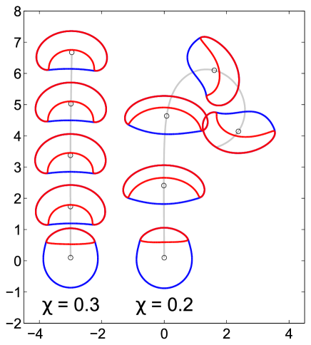
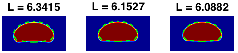
We numerically evaluate Eqs. 8-10 by a semi-implicit Fourier spectral method; see Appendix A for numerical details. We find that this simple model supports both straight and circular trajectories (Fig. 1). Initially the cell shape is taken to be circular, and we choose the -distribution to be polarized, in the front half and zero in the rear, though with a random noise added on top (Appendix A). Due to this -polarization, the front half of the cell is pushed out while the rear half is contracted, deforming the cell. After nearly , the crawling cell with reaches an equilibrium shape and undergoes a straight trajectory, while the one with undergoes a turning instability and transitions to a circular trajectory at . The straight trajectories resemble the highly persistent, half-moon shape of crawling keratocytes verkhovsky1999self ; keren2008mechanism ; barnhart2011adhesion . The turning behavior is equally likely to occur in either direction, and depends on the noise in the initial conditions; larger noise can accelerate turning, while states with zero initial noise can proceed for a very long time without turning.
While we show only cells that effectively crawl in Fig. 1, we also note that even initially polarized cells may become depolarized, with becoming uniform over the cell. This occurs at larger tensions than we plot here, in which the cell cannot effectively push the membrane out, and becomes too small to develop polarization. This corresponds to violations of the constraints in Eq. 11 in which wave-pinning fails mori2008wave ; jilkine2009wave , and only homogeneous solutions to the reaction-diffusion equations are possible.
V Transition to circular trajectories
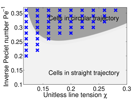
What parameters control the transition from straight trajectories to circular ones? We show a - phase diagram in Fig. 2; in this phase diagram, blue crosses indicate the parameters at which we have observed cells turning and following circular trajectories. In general, the straight trajectory is stabilized by increasing the unitless tension on the cell and decreasing the unitless diffusion coefficient of the diffusing molecule .
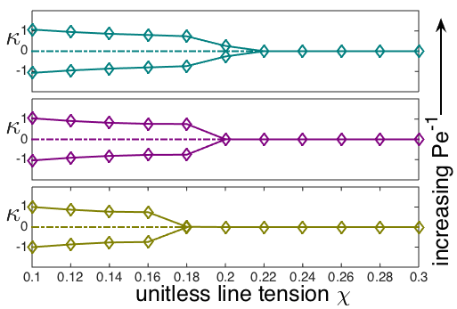
Additionally, for a crawling cell in circular trajectory, the curvature of the trajectory is affected by and . We show a bifurcation diagram of as a function of for three values of in Fig. 3. Curvature indicates the straight trajectory of the crawling cell. We see the existence of a supercritical pitchfork bifurcation point for below which the crawling cell tends to undergo circular motion (the up-down symmetry in the bifurcation diagram is due to the fact that the cell can turn to clockwise circular motion or counterclockwise circular motion with equal probability), and after which the cell becomes stable in a straight trajectory. The dashed line indicates that for small value of , the straightly crawling cell is unstable in the sense that it will turn to a circular motion under small perturbation in the system. As increases, the bifurcation value of becomes smaller, which is also observed in the phase digram Fig. 2.
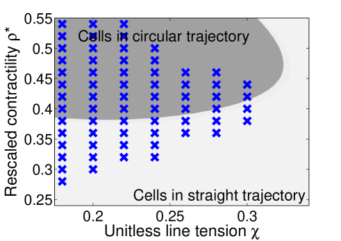
We plot a phase diagram for cell turning as a function of tension and rescaled contractility in Fig. 4; again, blue crosses indicate where the cell turns to a circular trajectory. Surprisingly, as we vary we observe reentry, as increasing first destabilizes the straight trajectory and then subsequently restabilizes it.
VI Origin of turning instability: analytical estimate of phase diagram
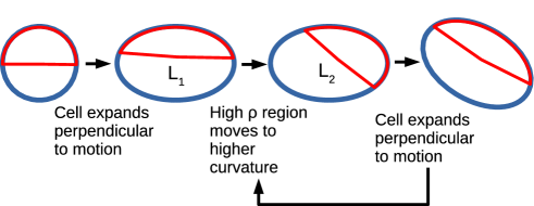
Why does turning occur? We argue that the turning instability and circular trajectory arise from the coupling between the reaction-diffusion mechanism and the cell shape in Eq. 9, in a scheme illustrated in Fig. 5. The reaction-diffusion mechanism tends to minimize the length of the interface between regions of high and low . For this reason, the high regions are attracted to high curvature vanderlei2011multiscale ; jilkine2009wave . As the cell is deformed, widening in the direction perpendicular to cell motion, the cell front becomes a local curvature minimum (Fig. 1), and the reaction-diffusion mechanism will, if the cell shape is fixed, re-orient the cell polarization to the high curvature region. The rate of this destabilizing process is controlled by the effective diffusion coefficient .
Given this instability, why can the cell maintain a straight trajectory if is low enough or high enough? Even if the polarity is linearly unstable, the straight trajectory may be rescued by the cell’s ability to adapt its shape. If the cell shape immediately reorients to any change in polarity, the cell cannot turn, and the straight trajectory is stabilized. This explain the importance of , as the dynamics of the cell shape strongly depend on . We would then naturally expect increasing to stabilize the cell, and increasing to destabilize it, as seen in Fig. 2. However, this intuition does not immediately explain the effect of in Fig. 4, which we will find to occur because of the influence of on cell shape.
We have been able to qualitatively, but not quantitatively reproduce the phase diagrams sketched in Fig. 2 and Fig. 4, including the reentry, with a calculation based on this argument. In Sec. VI.1, we show that the dynamics respond to the cell shape, and show that this instability is slower as Pe increases, but also depends on the cell shape. In Sec. VI.2, we study the dynamics of how the cell shape is controlled by the distribution of , and show that the speed at which a cell relaxes to its new shape is proportional to . In Sec. VI.3, we combine these results to predict the phase diagram of cells as a function of the effective cell tension , the Peclet number, and the rescaled contractility .
VI.1 Dynamics of Rho GTPase within a fixed geometry
Simulating the reaction-diffusion dynamics of Eq. 9 in a fixed, non-moving cell shows that the reaction-diffusion mechanism is sensitive to cell shape (Fig. 6). In particular, we find that the cell “front” (region of high ) rotates to point toward the higher-curvature region of the cell. This is consistent with the idea that the reaction-diffusion dynamics of Eq. 9 serve to minimize the interface between high and low . This behavior has been noted before jilkine2009wave ; vanderlei2011multiscale ; see also a brief discussion of this point in wolgemuth2011redundant .
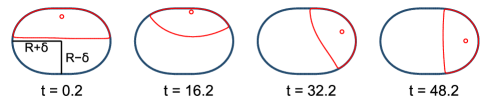
We characterize the kinetics of the instability of large moving to higher curvature, and how it depends on the cell shape and Peclet number. We will look at the dynamics of in a cell with a fixed shape,
where is, as usual, the angle counter-clockwise from the axis. To compute the evolution in in a fixed cell shape, we solve only Eq. 9 with a fixed , where is the (signed) distance from the curve .
The instability in Fig. 6 is a linear instability. We find that if the distribution of is initially centered near , we find an exponential increase of the center of mass of with time, . (Here, we define to be the angle to the center of mass of the distribution , .) If this instability is driven by the mean curvature flow identified by Ref. jilkine2009wave, , we would expect that . We have confirmed this numerically for the parameters we have studied (Fig. 7).
We also expect that as , the instability should vanish as a perfect circle has no shape asymmetry. We find, consistently with this intuition, that at small (Fig. 7). Based on these results, we hypothesize that with a constant, i.e.
| (12) |
Though this is reasonable at small , we would not expect it to necessarily generalize to larger aspect ratios. In addition, in a more complex shape, may depend on higher Fourier modes in the cell shape.
VI.2 Dynamics of cell shape response to
VI.2.1 Sharp interface theory
In the absence of any driving forces, or , the phase field Eq. 8 is simply an Allen-Cahn equation. In the sharp interface limit of , the interface evolves with a normal velocity with the interface curvature elder2001sharp (we note this is distinct from the curvature of the trajectory, which we also have labeled above, but is not addressed in this section). The added forcing terms correspond to the interface being advected with velocity where is the outward-pointing normal. Since this term varies smoothly across the boundary, we can get the normal interface velocity by adding directly to the curvature-driven relaxation velocity han2011comprehensive . Then the normal velocity of the cell boundary in arc-length should be:
| (13) |
When the cell takes on a steady shape, the normal velocity must satisfy:
| (14) |
where the integral is over the entire cell boundary.
VI.2.2 Steady cell shape in quasi-circular Fourier modes
Let us describe a cell with boundary given by the function , where the angle is with respect to the axis . We can expand in Fourier modes:
| (15) |
Here we assume that the cell shape is close to circular, , and we use to denote . The mode is excluded because it corresponds to the cell translational motion, which we include by assuming that the cell is initially traveling with a constant speed of . We have also excluded the size expansion mode; we find, in a numerically exact solution of Eq. 13, that there are many distinct solutions corresponding to different cell perimeters. Selecting or equivalently chooses which of these steady state solutions we observe, and will be done later by setting the cell perimeter .
The normal velocity at an angle is ohta2009deformation
| (16) |
Up to the first order of the deviations, we have
| (17) | ||||
| (18) |
Expanding Eq. 13 into Fourier modes, we find (assuming the cell has velocity ),
| (19) | ||||
We will treat and as zero when they arise from the term proportional to here, and
| (20) |
is the Fourier transform of the protrusion strength – how far the Rho GTPase protein exceeds the critical value .
The equations of motion for the Fourier modes (Eq. 19) depend on the velocity of the cell, . This velocity can be found, following ohta2009deformation , as
| (21) | ||||
| (22) |
where is the vector pointing from the cell’s center of mass to the element at arclength , is the cell area, and the approximation is true for small deformations.
We have seen from our simulations and the analysis of mori2008wave ; mori2011asymptotic that has a sharp interface between values and , which are controlled by the details of the reaction term Eq. 9. We thus assume a simple form for :
| (23) |
with indicating the angle of the cell over which is equal to , with . With this form,
| (24) |
Importantly, we can find without explicitly solving the reaction-diffusion equations. Integrating Eq. 13 over the arc-length and using Eq. 14, we find a relationship between , the cell shape, and that is required for there to be a steady state shape,
| (25) |
where is the cell perimeter. The integral over the arc length can be cast into one over the angle :
| (26) | ||||
| (27) |
then the Eq. 25 becomes, up to linear order in ,
| (28) |
This equation is a link between cell shape and at steady state. Expanding in as , where we assume is , we find
| (29) |
and
| (30) |
Then the Fourier modes of in Eq. 24 becomes, to linear order again,
If we look for the steady state of , which we will write , we find that, using Eq. 19,
| (31) | |||
which can be re-written as a simple matrix multiplication,
| (32) |
where
where is the Kronecker delta. Because multiplies terms of order , we can approximate it by
| (33) | ||||
| (34) |
to zeroth order in (Eq. 22).
Eq. 32 may be solved to reconstruct , and therefore , by truncating to finite number of Fourier modes, . If we only take the modes, the answer is relatively simple,
| (35) |
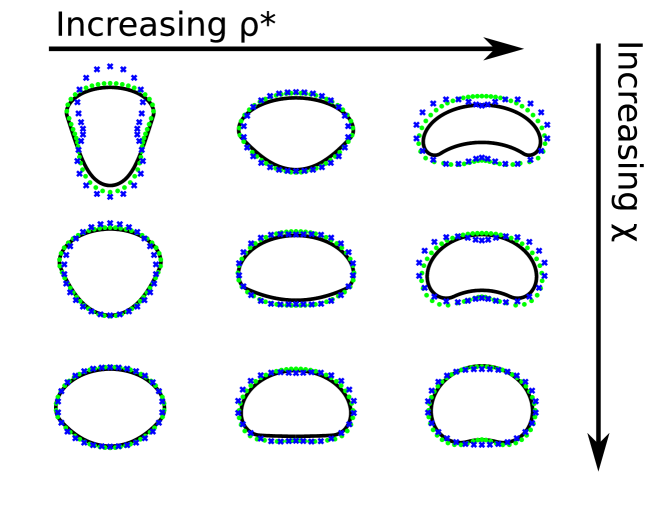
This model, with the assumptions we have made, is straightforward to solve. However, it is not numerically exact because of the assumption of quasi-circularity, . We compare the Fourier series shapes with a sharp-interface determination of the cell shape that does not require assuming in Appendix B.1.
VI.2.3 Dynamics of Perturbation from Steady-state Shape
In calculating the steady-state shape above, we have assumed that the cell travels at a steady velocity in the direction. Our simulations show that turning begins from a near-steady-state shape. To study this linear instability, we will calculate how the cell shape relaxes if we slightly change the distribution of . If the orientation of changes by a small angle , this is exactly the same as if we slightly rotate our cell shape away from the -axis, and see how it relaxes. We assume that this process is dominated by the dynamics of the lowest mode, ; we will thus look at the dynamics of when it takes on the form with small, and neglect all other modes . We will also assume that and do not depend on . With these assumptions, we find from Eq. 19 that, to linear order in ,
| (36) |
We note that because we have limited ourselves to the modes, the relaxation dynamics of this rotation do not depend on the cell’s velocity .
VI.3 Predicted Phase Diagram
We can now predict when the cell should be stable or unstable. Small perturbations of cell shape away from the direction of polarity relax with a rate , as shown in Eq. 36. We also found numerically that, in a fixed cell shape with a distortion size of , the front of the cell will move toward the narrow end of the cell with a rate (Fig. 7 and Eq. 12). Combining these results will show when the linear cell motion remains stable.
In our earlier results, computing the shape relaxation, we assumed that the initial direction of polarity was , but this is not necessary. Similarly in computing the instability of in a static cell shape, we assumed a stationary shape that is narrowed along the -axis, but we can rotate to consider the shape relative to an arbitrary axis to get equivalent results. We can then generalize our above results to
| (37) | ||||
| (38) |
Combining these equations, we find that the linear stability of , i.e. the difference between the direction of chemical polarity , and the direction of shape polarity, , is controlled by
| (39) |
from which we can see that when , we expect our straight-crawling cell to be stable to linear perturbations, and for we expect it to turn.
We established that . Using our simulations (Fig. 7), we estimate . The only other crucial feature is the steady-state shape of the crawling cell , which we know by Eq. 35 – assuming once again that the cell shape is dominated by the lowest mode. We then have the bifurcation relation for marginal stability:
| (40) |
where and is set by Eq. 29.
We show slices of this phase diagram in Fig. 2 and Fig. 4. The phase diagrams we compute are only roughly accurate, as would be expected with the number of approximations that we have made. However, we predict correctly both the order of magnitude of the transitions, and that there should be a reentry as decreases, where for both small and large there is stability (Fig. 4). However the theory also predicts a reentry for small ; this has not been observed in the simulations. This may be because as the tension becomes smaller, the cell shape becomes less and less quasi-circular, and our assumptions fail.
VII Discussion
We argue that the existence of turning and circular motion may be quite generic in cell motility of the sort we have studied here, with biochemical polarity mechanisms that create a single front. Many other reaction-diffusion dynamics or other potential biochemical models of the cell’s polarity jilkine2011comparison may display the attraction to high curvature which drives the instability we discuss here. For instance, polarity driven by phase separation of two non-miscible species zamparo2015dynamic would also tend to minimize the interface between these species. Related mechanisms, including phase separation, and the constrained Allen-Cahn equation, are known to display instabilities similar to that of Fig. 6 within fixed geometries alikakos2000motion ; stafford2001dynamics ; alikakos2000mullins ; marenduzzo2013phase . Turing patterns may also be reoriented by curvature, though in some reaction-diffusion systems, coupling to curvature can be overwhelmed by initial conditions orlandini2013domain ; vandin2016curvature . We also note that the coupling between shape and protein dynamics has been emphasized recently in a Rho GTPase model wave pinning model applied to dendritic spines ramirez2015dendritic , and cell shape-biochemistry interactions have been observed in a broad range of models and experiments camley2013periodic ; holmes2012modelling ; meyers2006potential . In general, we would expect any mechanism for that displays an effective line tension at the region between high and low to be able to generate turning instabilities of the type studied in our paper.
In addition, Ohta and Ohkuma ohta2009deformable have argued from a simple model proposed on symmetry grounds that the transition to circular motion is a generic property of active deformable particles, as long as there is a coupling between particle shape and particle polarity. Our model provides a possible example of this coupling in the context of cellular motility. However, the details of our mechanical model shows that generic models of this sort (e.g. ohta2016simple ; tarama2013oscillatory ; tarama2012spinning ; menzel2012soft ; hiraiwa2010dynamics ) can conceal surprises like reentry – it is not at all straightforward to map physical properties of cells into the effective parameters. In particular, because the destabilizing effect of the reaction-diffusion mechanism depends on the steady-state cell shape, any parameter that controls cell shape can alter the stability diagram, and cell shape may not be a simple monotonic function of changing physical parameters.
Cell turning has been studied in other models maree2006polarization ; mogilner2010actin , though primarily in a response to an altered stimulus – e.g. the rotation of a chemoattractant gradient or an actin asymmetry. This is in contrast to our example, where turning occurs spontaneously. However, we do note that Ref. maree2006polarization, , observes a drifting behavior which could be a transition into a very large-radius circular turn.
We have also observed turning and circular motion in the full model of shao2012coupling ; camley2013periodic , which includes fluid flow, separate dynamics for myosin, and individual adhesions with stochastic transitions: see Fig. S1 in the Supplementary Material of camley2013periodic . We have found that decreasing ( in camley2013periodic ) also tends to stabilize the cell in the more complex model. However, mechanical parameters do not have as straightforward an effect as studied in the simple model Eq. 8-10; in particular, we were unable to stabilize turning cells by straightforwardly increasing tension.
How do our results on turning and circular motion compare with experiments on cell motility? Recent work has shown that multi-lobed keratocytes undergo circular motion raynaud2016minimal , but with a very different shape than the cells we simulate. In addition, Gorelik and Gautreau have recently suggested that arpin dang2013inhibitory may induce cells to turn by slowing them gorelik2015arp2 ; this is consistent with our result that slowing the cell (or decreasing the Peclet number) can cause turning. However, we emphasize that in other cell types turning is associated with different morphology and may not be controlled by the simple mechanism studied here liu2015linking .
We predict, based on our analysis, that when our mechanism applies, cell slowing will correspond with increased turning, but by a different mechanism than the speed-persistence relationship identified by maiuri2015actin . Turning could potentially be prevented by reducing the membrane diffusion coefficient of polarity proteins on the surface of the cell, e.g. by increasing their binding to the cortex. We also argue that cell shape is a crucial mediator of turning: wider cells would, in this mechanism, tend to be less stable. Any interventions that alter cell tension, contractility at the cell rear, or strength of protrusiveness, and thereby alter cell shape may disrupt or induce turning.
VIII Conclusions
In this paper, we have presented a simplified variant of a phase field cell motility model, extending our earlier work shao2010computational ; camley2014polarity . We demonstrated that our model can support both straight and circular trajectories, with the circular trajectories occurring through a turning instability. We have argued that this instability occurs because of the instability of the protein dynamics model we have adapted mori2008wave that tends to orient proteins within the cell toward the cell’s narrower ends. When combination of the protein dynamics and cell shape dynamics leads to the cell widening, this may lead to destabilization of the straight trajectory. Both our model and our simple theory suggest that the phase diagram of turning can be highly complex, with changing parameters having non-monotonic effects on the stability: we observe that increasing contractility first destabilizes and then restabilizes the cell’s straight trajectory.
Appendix A Numerical Method
For the numerical method of the phase field model (Eqs. 8-10), we adopt the semi-implicit Fourier spectral method.
Let us consider a rectangular domain in :
and a periodic boundary condition is imposed for the problem. Let us discretize the spatial domain by a rectangular mesh which is uniform in each direction as follows:
for and , and . Let , denote the approximate solutions. Then the set of unknowns are
The Laplacian operator in the spectral space corresponds to the following spectrum
with
For the Eq. 8, we can write it into the semi-implicit form:
By taking the fast Fourier transform of both sides of the above equation, we get
where and stands for element-wise multiplication between matrices. The approximate solution of at can be obtained by taking inverse Fourier transform:
Similarly for the Eq. 9, we can write it into the semi-implicit form in terms of ,
and then apply the FFT and iFFT to find the approximate solution of at . The approximate solution at is obtained by:
In our numerical simulations, we take , and .
A.1 Initial Conditions
Initially the cell shape is taken to be circular with radius , with , and the -distribution equal to 0.8 in the front half and 0 in the rear half, with an added normally-distributed noise with standard deviation of 0.2.
Appendix B Sharp interface models without the quasi-circularity assumption
B.1 Exact Calculation of Steady-state Shapes of Straight Cells
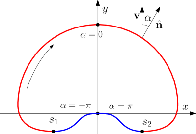
We can find a numerically exact solution to the steady-state shape of the cell by integrating the sharp-interface equation Eq. 13; related approaches, including graded radial extension models, have been applied before keren2008mechanism ; adler2013closing . If we assume that the cell is crawling along a straight trajectory with constant velocity , where stands for the unit -axis direction, then the relation between the cell velocity and cell shape can be obtained from Eq. 13:
| (41) |
where is the angle counterclockwise from to v, see Fig. 8, and the overhead dot represents the derivative with respect to the arc-length . We take the boundary conditions
| (42) |
which are appropriate if the cell perimeter is a simple closed curve, and there is no cusp at (Fig. 8). Given a solution , we can find the cell shape by integrating the tangent vector along the arclength,
| (43) |
Because the cell is a simple closed curve, we will find that and .
The only unknown parameter in Eq. 41 is the cell’s velocity , if we specify the cell perimeter. The two boundary conditions of Eq. 42 on the first-order equation of Eq. 41 shows that, for a fixed value , there will be only a particular value of for which Eq. 41 can be solved.
We know from our simulations and the analysis of mori2008wave ; mori2011asymptotic that has a sharp interface between values and :
| (44) |
where , and is the length of the region, see Fig. 8 in which the red part stands for the region. How large is ? Integrating Eq. 41 along the arc-length and using Eq. 14, we find that
and then
| (45) |
In practice, and are appropriate for our reaction-diffusion equations.
Eq. 41 coupled with the boundary conditions of 42 is numerically solved by using a shooting method to determine the value of for which the equations can be solved. As an example, we choose . We compare this result with our quasicircular approximation in Fig. 9, seeing generally good agreement on cell shape and size. Even using the model with only Fourier modes, we capture the appropriate trends of cell shape. We choose in the quasicircular approximation (Eq. 15); this is set so that the cell’s contour length in the quasicircular approximation matches that for the numerically exact method. (We note that the agreement between contour lengths is only approximate, and the contour length of some cells shown in Fig. 9 can deviate from .) Velocities predicted by the Fourier model are also in good agreement with those predicted by the numerically exact model, with errors of less than 25% for the parameters shown in Fig. 9, even only including modes.
The sharp interface solutions also have good agreement with the phase field solutions (Fig. 10). However, this agreement depends on the validity of our assumptions, e.g. that the value of at the cell front is unity. This is controlled by . Mathematically, resembles a penalty constant to maintain (Eq. 9). As becomes greater, becomes closer to and the phase field cell shrinks to the sharp interface one.
B.2 Exact Calculation of Steady-state Shape of Cells with Circular Trajectories
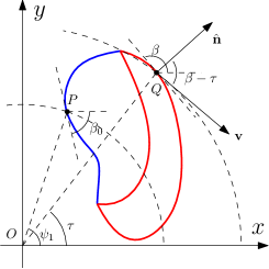

While we only used the sharp-interface results in the main paper to determine the steady-state shape of cells on straight trajectories, our techniques can also be used to determine the shape of cells undergoing circular motion. Schematically, we show a circularly moving cell in steady state in Fig. 11. The origin is the center of rotation, is a representative point on the cell boundary, is the angle made by from horizontal, is the angle of inclination from horizontal, is the normal to the cell boundary, and v is the moving direction of which is normal to . The blue curve represents the region and the red part is region. The point is the middle point of the blue region with respect to arc-length and is taken as the starting point for arc-length parameterization, namely, at . Note that the cell shape is independent of angle , so in the sharp-interface model, we take to keep on the -axis. The angle between and v is and the normal velocity
| (46) |
where is the constant angular velocity for the cell in circular steady state. Then in the circular steady state, we have
| (47) |
Notice that
Integrating Eq. 47 along the arclength, we find that
exactly as what we obtain from the equation for the straightly moving cell.
Finally we obtain the system for steady state of circular cells:
| (48) | ||||
with the following boundary conditions
| (49) | ||||||||
| (50) |
Note that for the boundary conditions (50) at , and automatically implies by considering (13), (14) and (48), so is a redundant boundary condition. Besides, the cell perimeter and the initial inclination angle are two unknown parameters, so the number of unknowns matches with the number of boundary conditions in (48-50). The length of the region is determined by Eq. 45, which is treated known once is determined.
Numerically, we solve the Eq. 48 coupled with boundary conditions (49-50) by a shooting method. The parameter values are , = 0.12 (0.18, respectively), = 1.0530 (1.3563, respectively) and = 0.5775 (0.3832, respectively) where the cell’s angular velocity and circular radius are taken from the phase field simulations (8-10). As in the earlier sharp interface limit calculations, we take . The numerical results are presented in Fig. 12 which have good agreement with the phase field simulations.
References
- (1) Dennis Bray. Cell movements: from molecules to motility. Garland Science, 2001.
- (2) Alex Mogilner and George Oster. Force generation by actin polymerization ii: the elastic ratchet and tethered filaments. Biophysical Journal, 84(3):1591, 2003.
- (3) Longhua Hu and Garegin A Papoian. Mechano-chemical feedbacks regulate actin mesh growth in lamellipodial protrusions. Biophysical Journal, 98(8):1375, 2010.
- (4) D. Shao, H. Levine, and W.-J. Rappel. Coupling actin flow, adhesion, and morphology in a computational cell motility model. Proceedings of the National Academy of Sciences, 109(18):6851, 2012.
- (5) B. Rubinstein, M.F. Fournier, K. Jacobson, A.B. Verkhovsky, and A. Mogilner. Actin-myosin viscoelastic flow in the keratocyte lamellipod. Biophysical Journal, 97(7):1853, 2009.
- (6) Marc Herant and Micah Dembo. Form and function in cell motility: from fibroblasts to keratocytes. Biophysical Journal, 98(8):1408, 2010.
- (7) Charles W Wolgemuth, Jelena Stajic, and Alex Mogilner. Redundant mechanisms for stable cell locomotion revealed by minimal models. Biophysical Journal, 101(3):545–553, 2011.
- (8) Athanasius FM Marée, Verônica A Grieneisen, and Leah Edelstein-Keshet. How cells integrate complex stimuli: the effect of feedback from phosphoinositides and cell shape on cell polarization and motility. PLoS Computational Biology, 8(3):e1002402, 2012.
- (9) Alexandra Jilkine and Leah Edelstein-Keshet. A comparison of mathematical models for polarization of single eukaryotic cells in response to guided cues. PLoS Computational Biology, 7(4):e1001121, 2011.
- (10) William R Holmes and Leah Edelstein-Keshet. A comparison of computational models for eukaryotic cell shape and motility. PLoS Computational Biology, 8(12):e1002793, 2012.
- (11) Falko Ziebert and Igor S Aranson. Computational approaches to substrate-based cell motility. npj Computational Materials, 2:16019, 2016.
- (12) Roman Gorelik and Alexis Gautreau. The arp2/3 inhibitory protein arpin induces cell turning by pausing cell migration. Cytoskeleton, 72(7):362, 2015.
- (13) Danying Shao, Wouter-Jan Rappel, and Herbert Levine. Computational model for cell morphodynamics. Physical Review Letters, 105(10):108104, 2010.
- (14) Y. Mori, A. Jilkine, and L. Edelstein-Keshet. Wave-pinning and cell polarity from a bistable reaction-diffusion system. Biophysical Journal, 94(9):3684, 2008.
- (15) Brian A Camley, Yunsong Zhang, Yanxiang Zhao, Bo Li, Eshel Ben-Jacob, Herbert Levine, and Wouter-Jan Rappel. Polarity mechanisms such as contact inhibition of locomotion regulate persistent rotational motion of mammalian cells on micropatterns. Proceedings of the National Academy of Sciences, page 201414498, 2014.
- (16) WJ Boettinger, JA Warren, C Beckermann, and A Karma. Phase-field simulation of solidification 1. Annual Review of Materials Research, 32(1):163–194, 2002.
- (17) Joseph B Collins and Herbert Levine. Diffuse interface model of diffusion-limited crystal growth. Physical Review B, 31(9):6119, 1985.
- (18) Thierry Biben, Klaus Kassner, and Chaouqi Misbah. Phase-field approach to three-dimensional vesicle dynamics. Physical Review E, 72(4):041921, 2005.
- (19) Falko Ziebert, Sumanth Swaminathan, and Igor S Aranson. Model for self-polarization and motility of keratocyte fragments. J. Roy. Soc. Interface, 9(70):1084–1092, 2012.
- (20) Jakob Löber, Falko Ziebert, and Igor S Aranson. Modeling crawling cell movement on soft engineered substrates. Soft matter, 10(9):1365–1373, 2014.
- (21) Jakob Löber, Falko Ziebert, and Igor S Aranson. Collisions of deformable cells lead to collective migration. Scientific Reports, 5, 2015.
- (22) Benoit Palmieri, Yony Bresler, Denis Wirtz, and Martin Grant. Multiple scale model for cell migration in monolayers: Elastic mismatch between cells enhances motility. Scientific Reports, 5, 2015.
- (23) Elsen Tjhung, Davide Marenduzzo, and Michael E Cates. Spontaneous symmetry breaking in active droplets provides a generic route to motility. Proceedings of the National Academy of Sciences, 109(31):12381, 2012.
- (24) E Tjhung, A Tiribocchi, D Marenduzzo, and ME Cates. A minimal physical model captures the shapes of crawling cells. Nature Communications, 6, 2015.
- (25) Yi I Wu, Daniel Frey, Oana I Lungu, Angelika Jaehrig, Ilme Schlichting, Brian Kuhlman, and Klaus M Hahn. A genetically encoded photoactivatable Rac controls the motility of living cells. Nature, 461(7260):104, 2009.
- (26) Marten Postma, Leonard Bosgraaf, Harriët M Loovers, and Peter JM Van Haastert. Chemotaxis: signalling modules join hands at front and tail. EMBO Reports, 5(1):35, 2004.
- (27) Julien Kockelkoren, Herbert Levine, and Wouter-Jan Rappel. Computational approach for modeling intra-and extracellular dynamics. Physical Review E, 68(3):037702, 2003.
- (28) X Li, J Lowengrub, A Rätz, and A Voigt. Solving PDEs in complex geometries: a diffuse domain approach. Communications in Mathematical Sciences, 7(1):81, 2009.
- (29) Brian A Camley, Yanxiang Zhao, Bo Li, Herbert Levine, and Wouter-Jan Rappel. Periodic migration in a physical model of cells on micropatterns. Physical Review Letters, 111(15):158102, 2013.
- (30) Alexander B Verkhovsky, Tatyana M Svitkina, and Gary G Borisy. Self-polarization and directional motility of cytoplasm. Current Biology, 9(1):11, 1999.
- (31) Kinneret Keren, Zachary Pincus, Greg M Allen, Erin L Barnhart, Gerard Marriott, Alex Mogilner, and Julie A Theriot. Mechanism of shape determination in motile cells. Nature, 453(7194):475–480, 2008.
- (32) Erin L Barnhart, Kun-Chun Lee, Kinneret Keren, Alex Mogilner, and Julie A Theriot. An adhesion-dependent switch between mechanisms that determine motile cell shape. PLoS Biology, 9(5):e1001059, 2011.
- (33) Kinneret Keren and Julie A Theriot. Biophysical aspects of actin-based cell motility in fish epithelial keratocytes. In Cell Motility, page 31. Springer, 2008.
- (34) Yasushi Sako, Kayo Hibino, Takayuki Miyauchi, Yoshikazu Miyamoto, Masahiro Ueda, and Toshio Yanagida. Single-molecule imaging of signaling molecules in living cells. Single Molecules, 1(2):159, 2000.
- (35) Alexandra Jilkine. A wave-pinning mechanism for eukaryotic cell polarization based on Rho GTPase dynamics. PhD thesis, University of British Columbia (Vancouver), 2009.
- (36) Takao Ohta and Takahiro Ohkuma. Deformable self-propelled particles. Physical Review Letters, 102(15):154101, 2009.
- (37) Ben Vanderlei, James J Feng, and Leah Edelstein-Keshet. A computational model of cell polarization and motility coupling mechanics and biochemistry. Multiscale Modeling and Simulation, 4(9):1420–1443, 2011.
- (38) KR Elder, Martin Grant, Nikolas Provatas, and JM Kosterlitz. Sharp interface limits of phase-field models. Physical Review E, 64(2):021604, 2001.
- (39) Tao Han and Mikko Haataja. Comprehensive analysis of compositional interface fluctuations in planar lipid bilayer membranes. Physical Review E, 84(5):051903, 2011.
- (40) Takao Ohta, Takahiro Ohkuma, and Kyohei Shitara. Deformation of a self-propelled domain in an excitable reaction-diffusion system. Physical Review E, 80(5):056203, 2009.
- (41) Y. Mori, A. Jilkine, and L. Edelstein-Keshet. Asymptotic and bifurcation analysis of wave-pinning in a reaction-diffusion model for cell polarization. SIAM Journal on Applied Mathematics, 71(4):1401, 2011.
- (42) Marco Zamparo, F Chianale, Claudio Tebaldi, M Cosentino-Lagomarsino, M Nicodemi, and A Gamba. Dynamic membrane patterning, signal localization and polarity in living cells. Soft Matter, 11(5):838, 2015.
- (43) Nicholas D Alikakos, Xinfu Chen, and Giorgio Fusco. Motion of a droplet by surface tension along the boundary. Calculus of Variations and Partial Differential Equations, 11(3):233–305, 2000.
- (44) Doug Stafford, Michael J Ward, and Brian Wetton. The dynamics of drops and attached interfaces for the constrained Allen–Cahn equation. European Journal of Applied Mathematics, 12(01):1, 2001.
- (45) Nicholas D Alikakos, Peter W Bates, Xinfu Chen, and Giorgio Fusco. Mullins-Sekerka motion of small droplets on a fixed boundary. Journal of Geometric Analysis, 10(4):575, 2000.
- (46) Davide Marenduzzo and Enzo Orlandini. Phase separation dynamics on curved surfaces. Soft Matter, 9(4):1178, 2013.
- (47) E Orlandini, D Marenduzzo, and AB Goryachev. Domain formation on curved membranes: phase separation or Turing patterns? Soft Matter, 9(39):9311, 2013.
- (48) Giulio Vandin, Davide Marenduzzo, Andrew B Goryachev, and Enzo Orlandini. Curvature-driven positioning of Turing patterns in phase-separating curved membranes. Soft Matter, 12(17):3888, 2016.
- (49) Samuel A Ramirez, Sridhar Raghavachari, and Daniel J Lew. Dendritic spine geometry can localize GTPase signaling in neurons. Molecular Biology of the Cell, 26(22):4171, 2015.
- (50) William R Holmes, Benjamin Lin, Andre Levchenko, and Leah Edelstein-Keshet. Modelling cell polarization driven by synthetic spatially graded rac activation. PLoS Computational Biology, 8(6):e1002366, 2012.
- (51) Jason Meyers, Jennifer Craig, and David J Odde. Potential for control of signaling pathways via cell size and shape. Current Biology, 16(17):1685–1693, 2006.
- (52) Takao Ohta, Mitsusuke Tarama, and Masaki Sano. Simple model of cell crawling. Physica D: Nonlinear Phenomena, 318:3, 2016.
- (53) Mitsusuke Tarama and Takao Ohta. Oscillatory motions of an active deformable particle. Physical Review E, 87(6):062912, 2013.
- (54) Mitsusuke Tarama and Takao Ohta. Spinning motion of a deformable self-propelled particle in two dimensions. Journal of Physics: Condensed Matter, 24(46):464129, 2012.
- (55) Andreas M Menzel and Takao Ohta. Soft deformable self-propelled particles. EPL (Europhysics Letters), 99(5):58001, 2012.
- (56) T Hiraiwa, MY Matsuo, T Ohkuma, T Ohta, and M Sano. Dynamics of a deformable self-propelled domain. EPL (Europhysics Letters), 91(2):20001, 2010.
- (57) Athanasius FM Marée, Alexandra Jilkine, Adriana Dawes, Verônica A Grieneisen, and Leah Edelstein-Keshet. Polarization and movement of keratocytes: a multiscale modelling approach. Bulletin of Mathematical Biology, 68(5):1169, 2006.
- (58) A Mogilner and B Rubinstein. Actin disassembly’clock’and membrane tension determine cell shape and turning: a mathematical model. Journal of Physics: Condensed Matter, 22(19):194118, 2010.
- (59) Franck Raynaud, Mark E Ambühl, Chiara Gabella, Alicia Bornert, Ivo F Sbalzarini, Jean-Jacques Meister, and Alexander B Verkhovsky. Minimal model for spontaneous cell polarization and edge activity in oscillating, rotating and migrating cells. Nature Physics, 12(4):367, 2016.
- (60) Irene Dang, Roman Gorelik, Carla Sousa-Blin, Emmanuel Derivery, Christophe Guérin, Joern Linkner, Maria Nemethova, Julien G Dumortier, Florence A Giger, Tamara A Chipysheva, et al. Inhibitory signalling to the Arp2/3 complex steers cell migration. Nature, 503(7475):281, 2013.
- (61) Xiaji Liu, Erik S Welf, and Jason M Haugh. Linking morphodynamics and directional persistence of T lymphocyte migration. Journal of The Royal Society Interface, 12(106):20141412, 2015.
- (62) Paolo Maiuri, Jean-François Rupprecht, Stefan Wieser, Verena Ruprecht, Olivier Bénichou, Nicolas Carpi, Mathieu Coppey, Simon De Beco, Nir Gov, Carl-Philipp Heisenberg, et al. Actin flows mediate a universal coupling between cell speed and cell persistence. Cell, 161(2):374, 2015.
- (63) Yair Adler and Sefi Givli. Closing the loop: Lamellipodia dynamics from the perspective of front propagation. Physical Review E, 88(4):042708, 2013.