Spectropolarimetric observations of an arch filament system
with the GREGOR solar telescope

Abstract

Arch filament systems occur in active sunspot groups, where a fibril structure connects areas of opposite magnetic polarity, in contrast to active region filaments that follow the polarity inversion line. We used the GREGOR Infrared Spectrograph (GRIS) to obtain the full Stokes vector in the spectral lines Si i $\lambda$1082.7 nm, He i $\lambda$1083.0 nm, and Ca i $\lambda$1083.9 nm. We focus on the near-infrared calcium line to investigate the photospheric magnetic field and velocities, and use the line core intensities and velocities of the helium line to study the chromospheric plasma. The individual fibrils of the arch filament system connect the sunspot with patches of magnetic polarity opposite to that of the spot. These patches do not necessarily coincide with pores, where the magnetic field is strongest. Instead, areas are preferred not far from the polarity inversion line. These areas exhibit photospheric downflows of moderate velocity, but significantly higher downflows of up to 30 km s^-1 in the chromospheric helium line. Our findings can be explained with new emerging flux where the matter flows downward along the fieldlines of rising flux tubes, in agreement with earlier results.

1 Introduction

The structure of solar filaments depends on the magnetic field at their photospheric footpoints. Thus, to understand the processes forming a filament, a good knowledge of the underlying magnetic vector field is mandatory. In active regions, one has to distinguish between active region filaments and arch filament systems (AFS). Active region filaments follow the neutral or polarity inversion line (PIL), while structures in AFS cross the PIL. Commonly, active region filaments are related to magnetic shearing at the PIL, and AFSs appear where the emergence of new flux is still ongoing. The physical processes that lead in both cases to dark structures in chromospheric lines need to be investigated in more detail. It is generally assumed that the dark structures of an AFS represent the emerging fluxtubes. In this work we investigate such an AFS. For active region filaments we refer to recent works of Kuckein et al. (2012a), Kuckein et al. (2012b), Sasso et al. (2014) and Schwartz et al. (2016) and references therein.

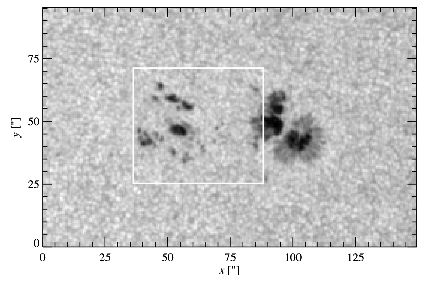
Figure 1: Intensity image taken at 08:16 UT by HMI. The white box outlines the area investigated in this work.

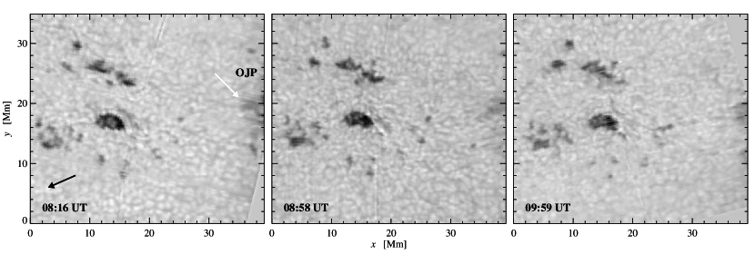
Figure 2: Temporal evolution of the slit-reconstructed continuum images. We apply an unsharp masking to enhance the displayed contrast. The black arrow points towards disk center and the white arrow to an outjutting part of the penumbra (OJP) of the nearby spot.

Howard & Harvey (1964) distinguished between filaments and fibrils, where filaments lie parallel to iso-contour lines of the magnetic field and fibrils traverse them perpendicularly. Martres et al. (1966) observed fibrils (“traces filamenteuses”) that connect areas of opposite polarity crossing the PIL. Systems of fibrils were described by Bruzek (1967), and he suggested to call them AFS. They appear in the inter spot area and connect spots of opposite polarities and cross the PIL. Strong downflows of about 50 km s^-1 occur at the footpoints of arch filaments (Bruzek 1969). The dynamic evolution of an AFS was investigated by Spadaro et al. (2004), who found upward motions in central parts of the fibrils and downward flows at their ends. Recently, Vargas Domínguez et al. (2012) used Hinode data to study AFS related to granular scale flux emergence in an active region. Grigor’eva et al. (2012) considered the formation of AFS in an active region as the onset of newly emerging flux before a strong flare occurred one day later. Ma et al. (2015) investigate an AFS in H$\alpha$, and they use magnetograms from the Helioseismic and Magnetic Imager (HMI) onboard the Solar Dynamics Observatory (SDO). In their case, the arch filaments are related to moving magnetic features of opposite polarity to that of the main sunspot and the arch filaments are controlled by the moving magnetic features. Solanki et al. (2003) and Lagg et al. (2007) observed an AFS in the infrared helium line at 1083 nm and determined its magnetic structure. The chromospheric magnetic field of another AFS is investigated by Xu et al. (2010). In the zone of flux emergence they find a magnetic field strength of 300 G, and the magnetic field is almost horizontal. At the edge of the emerging zone, the field is more vertical and stronger with a field strength of up to 850 G. Supersonic downflows occur at both footpoints of a fibril (or loop as the authors call the structures).

In the present work, we investigate an AFS, and we will concentrate on the magnetic field and the Doppler velocities in the lower photosphere. According to Howard & Harvey (1964) we will use the term “fibril” instead of “arch filament” for the single structures of the AFS in this work. Results of the upper photosphere and chromosphere will be topic of another article, except for a velocity determination from the infrared helium triplet line at $\lambda$1083 nm.

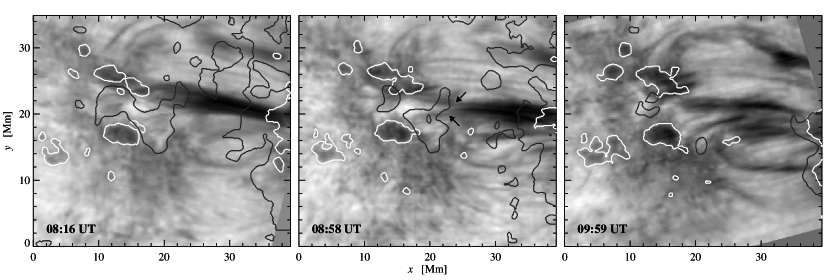
Figure 3: Temporal evolution of the slit-reconstructed helium line core intensity. White contours mark the dark photospheric intensity structures as seen in Fig. 2, and the black ones indicate the PILs. The small arrows in the mid panel indicate the splitting of the main fibril.

2 Observations

A small AFS in active region NOAA 12353 was observed on 2015 May 24 at the 1.5-meter GREGOR solar telescope (Schmidt et al. 2012; Kneer 2012; Denker et al. 2012). The whole group is depicted in Fig. 1. It was located at $x=380\arcsec$ and $y=140\arcsec$, corresponding to cos$\vartheta$ = 0.904. The image was stabilized and corrected in real-time by the GREGOR Adaptive Optics System (GAOS, Berkefeld et al. 2012). The AO system locked on the central pore in the marked subfield of Fig. 1.

We used the GREGOR Infrared Spectrograph (GRIS, Collados et al. 2012) in spectropolarimetric mode. More details about the polarimeter are presented in Collados et al. (2007). The spectral range was 1082.4 – 1084.2 nm which covers the silicon line $\lambda$1082.7 nm from the upper photosphere, the chromospheric helium triplet $\lambda$1083.0 nm and the calcium line $\lambda$1083.9 nm from the deep photosphere. The silicon and the calcium lines are both Zeeman triplets with an effective Landé-factor of $g_{\mathrm{eff}}=1.5$. The spectral dispersion was 1.810 pm per pixel, and the spectral resolution element is 5.7 pm assuming the measured resolution power given by Collados et al. (2012). Lagg et al. (2016) re-determined the spectral resolution power in a lower order to 110 000 very close to the value of Collados et al. (2012). We scanned five times across the region with the slit scanner in the time interval 08:06 – 10:08 UT. The step size was 0135, and a scan consisted of 400 steps, except for the first scan when we carried out 450 steps. We covered roughly 60^′′ along the slit. The single exposure time was 100 ms, and we accumulated four cycles through the different states of the ferro-electric liquid crystals. A scan of 400 steps thus takes about 18 min.

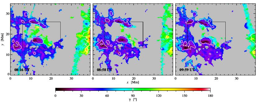
Figure 4: The inclination of the magnetic field strength for three different scans. White contours indicate the dark photospheric structures. The rectangular boxes indicate the area over which we integrated the negative magnetic flux, see text. In the gray areas, the polarization signal is below the significance threshold.

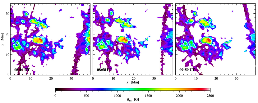
Figure 5: The total magnetic field strength for three different scans. White contours indicate the dark photospheric structures. In the white areas, the polarization signal is below the significance threshold.

3 Data reduction

The data were corrected using dark and flat-field frames. The polarimetric calibration was carried out with measurements taken with the GREGOR Polarimetric calibration Unit (GPU, Hofmann et al. 2012). The demodulation of the measurements follows the description by Collados (1999). A crosstalk correction is performed similar as described by Collados & Schlichenmaier (2002) for the VTT, but for the GRIS-data, only the influence of Stokes $I$ on $Q$, $U$ and $V$ is corrected to force the continuum in the polarization parameters to zero. No correction for the crosstalk between linear and circular polarization is applied. To derive the magnetic vector field, we use the code Stokes Inversion based on Response functions (SIR, Ruiz Cobo & del Toro Iniesta 1992). Since the calcium line is rather weak, it forms in a narrow atmospheric height layer, and we can restrict the calculation to one node for Doppler velocity, magnetic field strength, inclination, and azimuth, and we keep these values height-independent. Only for the temperature, we do allow three nodes. We assumed a single atmospheric component. The dispersed straylight was kept fixed at a level of 2%. This value seems to be rather low, but we found the fits to be more reliable than with a significantly higher amount of straylight. The true amount of straylight is probably higher, but in our case the assumption of unpolarized light from the non-magnetic quiet sun, as only foreseen in the SIR-code, is insufficient.

Photospheric Doppler shifts suffer from temporal spectrograph drifts. We assume that the wavelength of a nearby telluric line caused by water vapor does not change, so that we can use it to correct for the spectrograph drifts. We determine its wavelength by applying a polynomial fit through the line core. The drifts correspond to several 100 m s^-1 during a single scan.

All maps shown in this article are compensated for the differential image rotation (for details see Appendix A). The magnetic vector is transferred to the local frame of reference. Then, all images are rotated as a whole to have the $y$-axis parallel to the solar North-South direction, and the geometrical foreshortening has been corrected. Finally, we cut out the common area as shown in Fig 2.

4 Results

The morphology and dynamics of AFS are closely linked to the photospheric and chromospheric flows and magnetic fields. A display of three slit-reconstructed continuum images is shown in Fig. 2. Since the evolution in the area was not too fast, we show only three of the five scans in this and the following figures. We scanned an area containing several pores of the following part of the group, while the main spot was just outside of this area. The AFS connected the main spot just outside at the right of Fig. 2 with following pores of opposite magnetic polarity (see Fig. 3). The fibrils were more or less perpendicular to the PIL. In the first scan, the AFS is rather compact and connects an outjutting (protruding) part of the penumbra (OJP), indicated by the white arrow in Fig. 2 with the merging pores at $x=10-20$ Mm and $y=26$ Mm. Then the AFS becomes weaker on the side towards the pores, and we see two branches, marked by little arrows in the mid panel of Fig. 3. The stronger branch now reaches the central pore at $x=20$ Mm and $y=18$ Mm. In the last scan the AFS separates into several substructures, and the OJP is no longer in the field of view. In addition, some arc structures, barely visible before, become more pronounced. The central pore did not change very much, but the two pores above were merging during our observing period. In the following, we present the results from near-infrared spectropolarimetry.

4.1 Magnetic field

The larger pores have a positive magnetic polarity corresponding to small values for the magnetic inclination as seen in Fig. 4. The leading spot has negative polarity, and there is negative polarity between the pores (inclination larger than 90^∘). The total magnetic field strength is displayed in Fig. 5. The central pore is the strongest one and contains fields of up to 2500 G. The two merging pores have cores with field strengths of about 2000 G in the first scan. Other pores have 1600 – 1800 G. Below the AFS, we encounter magnetic fields with 200 – 400 G, and the vertical component is less than 100 G with varying sign. The magnetic field at the edge of the penumbra amounts to 900 – 1000 G. In the OJP, the vertical component of the magnetic field amounts to values between $-300$ and $-200$ G, as expected for a spot with negative magnetic polarity. At 08:16 UT, the magnetic field in the OJP is almost horizontal ( 100^∘), but at 08:58 UT, it is more vertical (140^∘ – 150^∘). In contrast, the nearby areas show a positive component of several hundred Gauss.

We estimate the positive magnetic flux in the pores and their surroundings and the flux of opposite sign in the intermediate area between the pores by integrating the vertical component of the magnetic field. The negative flux between the pores is integrated in the rectangular subfield with the coordinates 5.9 Mm $<x<$ 24.6 Mm and 13.2 Mm $<y<$ 26.0 Mm, which is indicated by the rectangles in Fig. 4. Both the area containing negative flux and the magnetic flux of negative sign decreases with time. The value of positive flux is increasing with time, but the errors are quite large. If real, this increase is much larger than the decaying negative flux. Values are given in Table 1.

Table 1: Magnetic flux in pores and intermediate area.

Scan	Time	positive flux	negative flux
		($10^{13}$ Wb)	($10^{11}$ Wb)
1	08:06 UT	1.5 $\pm$ 0.5	$-5.2$ $\pm$ 2.6
2	08:27 UT	1.2 $\pm$ 0.4	$-3.2$ $\pm$ 2.2
3	08:58 UT	1.7 $\pm$ 0.5	$-2.8$ $\pm$ 1.3
4	09:36 UT	1.8 $\pm$ 0.5	$-0.8$ $\pm$ 0.9
5	09:59 UT	1.8 $\pm$ 0.6	$-0.6$ $\pm$ 0.8

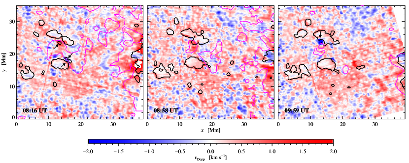
Figure 6: Doppler velocities determined from the photospheric calcium line. The black contours mark the dark photospheric structures and the magenta contours indicate the PILs. Values larger than 2 km s^-1 are clipped. Little arrows indicate special patches discussed in the text.

4.2 Photospheric Doppler velocities

Photospheric Doppler velocities are displayed in Fig. 6. Inside the central pore, we encounter very low velocities, but at the edge towards the opposite magnetic polarity, we see a patch of redshifts and just outside at the PIL blueshifts, which might indicate a horizontal flow roll. These patches are marked by little arrows in Fig. 6, as well as the following one. At the edge of the two merging pores, where the dark fibrils end, the line is redshifted during the scans at 08:16 UT and at 08:58 UT (about 2 km s^-1 in the beginning). In the last scan at 09:59 UT, we find a blueshift of about $-2$ km s^-1 instead of the previously observed downflow. The OJP exhibits mainly a blueshift of about $-0.5$ km s^-1. A blueshift here is in agreement with the expected Evershed effect, because the disk center is towards the left. However, on both sides of the OJP, we see strong redshifts up to 5 km s^-1 inside the penumbra. A similar configuration was described by Schlichenmaier et al. (2011) and Schlichenmaier et al. (2012), in that case it was observed during the formation of the penumbra. In the intermediate area between the main spot and the pores, we find dominantly redshifts in the order of 0.4 – 1 km s^-1.

4.3 Chromospheric Doppler velocities

Chromospheric Doppler velocities are determined from the helium line by applying the method introduced by González Manrique et al. (2016). The velocities are calibrated on an absolute scale following the steps in Appendices A and B of Kuckein et al. (2012b). Here, we present the results for a one-component line fit. Upflows (blueshifts) amount to up to 5 km s^-1 and appear mainly with an arch-like structure between the main spot and the opposite polarity pores. In general, these blueshifts do not coincide with the PIL of the deep photosphere. Downflows (redshifts) reach values up to 30 km s^-1. In the beginning at 08:16 UT, they occur next to the end of the most pronounced arch at the merging pores. We also find a redshift above the penumbra, while there is a blueshift in the OJP, in the photosphere caused by the Evershed effect (see Fig. 6). Later we encounter the maximum values between the central pore and the merging ones hitting the polarity inversion lines. The results are displayed in Fig. 7. A similar distribution of strong redshifts (up to 15 km s^-1) at the footpoints of magnetic loops and moderate blueshifts (up to -5 km s^-1) in their central parts was observed by Lagg et al. (2007).

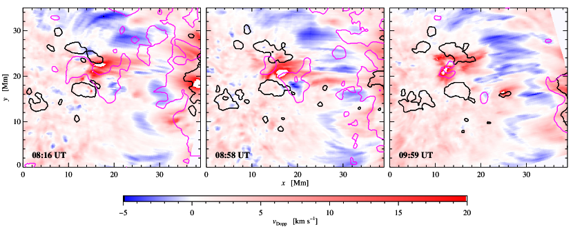
Figure 7: Doppler velocities determined from the helium line. The velocities are limited to 20 km s^-1, i.e., in the white patches they reach up to 30 km s^-1. Black contours indicate the dark photospheric structures and magenta ones the photospheric PILs.

5 Discussion

We examine an AFS, where the fibrils cross the photospheric PIL, and it is likely that the fibrils connect areas of different polarities, in contrast to active region filaments that follow the PIL. AFSs are related to new emerging bipolar magnetic flux. We conjecture that the physics behind the fibrils described by Howard & Harvey (1964) and the arch filaments observed by Bruzek (1967) is very similar, and that the difference lies in their appearance in H$\alpha$. Unfortunately, we do not have H$\alpha$ data taken in parallel to our observations.

In the beginning of our observations at 08:16 UT, the dark fibrils connect apparently the OJP, where we see the normal Evershed effect in photospheric layers, with the region next to the merging pores, where the matter is flowing downward. Next to the OJP, we encounter redshifts, probably downflows. In the helium line, we see downflows above the penumbra, but the strongest downflows appear at the other footpoints of the fibrils. These chromospheric downflows correspond probably to the photospheric downflows next to the OJP. However, Schad et al. (2013) find that is rather difficult to connect the involved height layers, even although they performed an inversion of the helium line. In the present state of our work, we do not know in which height layer the helium line is formed, perhaps so high that there is a big spatial gap to the photosphere. The magnetic field in the OJP becomes less inclined with time, and at the end of our observations, the OJP is no longer in the field of view. It seems that this area plays an important role for the understanding of the fibrils that are dark in the helium core, but for sophisticated conclusions we would need the results from different atmospheric layers that we do not have already for this paper. The fibrils seem to end in most cases at patches with opposite polarity to that of the main spot, but at locations that are not very far from the PIL. These patches do not necessarily coincide with the dark pores, where the magnetic field is strongest.

Possibly, rising bipolar flux cancels the negative magnetic polarity between the pores. The positive magnetic flux in the pores remains more or less constant, but the negative flux in this area decreases. Ultimately, the negative flux in the spot itself should increase, but we cannot confirm this because the spot itself is outside our field-of-view.

6 Conclusions

We observe blueshifts (upflows) in the helium velocities along the central part of the fibrils, which hints at rising flux tubes. At their summits, matter can move only along the field line, and thus the matter has to rise with the flux tube. At the footpoints of the flux tubes we see a downward motion. These results are in qualitative agreement with previous results obtained by Bruzek (1969), Solanki et al. (2003), Spadaro et al. (2004), Lagg et al. (2007) and Xu et al. (2010). Since we observe redshifts at both ends of the fibrils, we can exclude a siphon flow, in that case one would expect a blueshift on one side. In total, this picture is in good agreement with the sketch of Bruzek (1969). The rising flux tube does not gain much matter by condensations out of the surroundings, and after a while, not enough matter remains to maintain the downward drain and to absorb light in the helium line. The fibrils are no longer visible, and the downflow ends. This process is repeated when a new flux tube emerges.

The analysis of the helium and silicon data is ongoing work, and we have to refer to a future work answering the question: How is the magnetic field oriented in the layers of the fibrils? The analysis of the helium and silicon data will shed more light on the connection between the deep photosphere to the chromosphere. In addition, we plan new observations to elucidate the physical properties of AFSs.

Appendix A Differential image rotation compensation

The alt-azimuthal mount of the GREGOR-telescope (Volkmer et al. 2012) causes an image rotation, which is not negligible even during a scan of just 18 min. In the future, this image rotation can be compensated by a derotator, which was not available during our observations. To compensate for the differential image rotation during a scan, an IDL routine was developed. We assume that GAOS is locking on a structure next to the center of the scanned area keeping the solar structure at this position. Thus, the apparent axis of rotation falls together with this position, and we leave the central slit position untouched. According to the telescope elevation and azimuth, we calculate the relative rotation angle for each scan position with respect to the central one. The ephemeris are calculated at five-minute intervals, and then these results are interpolated to the exact time of each scan step. Next, we calculate the true position of each observed pixel within the map. Finally, we interpolate the map to a grid, which is equally spaced in seconds of arc along the two directions. Since we keep the orientation of the central slit position, a rotation of the whole image is still needed to orient the map with respect to the solar North-South direction. Thus, a rotation by a quite large angle might be required, while the differential rotation adds up to only a few degrees. Therefore, we separate these two steps. This routine will be included in the sTools IDL software library, which AIP’s solar physics research group develops in the framework of the EU-funded SOLARNET project for “High-Resolution Solar Physics”. For the present work, we apply this routine to the results of the SIR inversion but not to the spectra to save computation time.

The source code can be obtained on request from the corresponding author.