Chiral corrections to the Adler-Weisberger sum rule

Abstract

The Adler-Weisberger sum rule for the nucleon axial-vector charge, $g_{\scriptscriptstyle A}$, offers a unique signature of chiral symmetry and its breaking in QCD. Its derivation relies on both algebraic aspects of chiral symmetry, which guarantee the convergence of the sum rule, and dynamical aspects of chiral symmetry breaking—as exploited using chiral perturbation theory—which allow the rigorous inclusion of explicit chiral symmetry breaking effects due to light-quark masses. The original derivations obtained the sum rule in the chiral limit and, without the benefit of chiral perturbation theory, made various attempts at extrapolating to non-vanishing pion masses. In this paper, the leading, universal, chiral corrections to the chiral-limit sum rule are obtained. Using PDG data, a recent parametrization of the pion-nucleon total cross-sections in the resonance region given by the SAID group, as well as recent Roy-Steiner equation determinations of subthreshold amplitudes, threshold parameters, and correlated low-energy constants, the Adler-Weisberger sum rule is confronted with experimental data. With uncertainty estimates associated with the cross-section parameterization, the Goldberger-Treimann discrepancy, and the truncation of the sum rule at $\mathcal{O}(M_{\pi}^{4})$ in the chiral expansion, this work finds $g_{\scriptscriptstyle A}=1.248\pm 0.010\pm 0.007\pm 0.013$.

1 Introduction

The success of the Adler-Weisberger (AW) sum rule Adler (1965); Weisberger (1965) in calculating the nucleon axial-vector charge, $g_{A}$, was important historically Adler (2006) as it provided a striking pre-QCD confirmation of the importance of chiral symmetry in understanding nucleon structure through the strong interaction. The original derivation of the sum rule used some of the language of the infinite momentum frame as well as then-available knowledge of current algebra low-energy theorems. These two technologies have substantially advanced and evolved, and therefore it is interesting to reassess the theoretical basis for the AW sum rule. In addition, knowledge of the experimental total cross-sections in the resonance region Workman et al. (2012)—which is essential for a confrontation of the sum rule with experiment—as well as overall knowledge of the pion-nucleon interaction Hoferichter et al. (2015) have advanced to a high level. Therefore, an updated analysis of the experimental validity of the AW sum rule and its implications for the nucleon axial-vector charge, with controlled uncertainties, is timely.

It is worth summarizing the standard view of how the AW sum rule is obtained. Firstly, soft-pion theorems are derived using current algebra methods or chiral perturbation theory Weinberg (1979); Gasser and Leutwyler (1984); Gasser et al. (1988); Jenkins and Manohar (1991); Becher and Leutwyler (2001) ($\chi$PT) to obtain the crossing-odd, forward scattering amplitude at a special low-energy kinematical point. The Regge model of asymptotic behavior is then invoked to argue that this amplitude vanishes sufficiently quickly at high energy to guarantee an unsubracted dispersion relation, and the optical theorem is used to replace the absorptive part of the scattering amplitude with the total cross-section. While there is nothing wrong with this perspective of the sum rule, one goal of this paper is to stress that it is not necessary to invoke Regge lore in deriving the AW sum rule de Rafael (1997), as the scattering amplitude in question is explicitly calculable in the Regge limit ($s\gg-t$), and is found to vanish as a consequence of the chiral symmetry of QCD Beane and Hobbs (2016); Weinberg (1969). The convergence of the AW sum rule is therefore a direct consequence of the chiral symmetry of QCD and does not depend on model input.

In the original derivations, the major theoretical hurdle in confronting the AW sum rule with experiment was the ambiguity in extrapolating from the world of massless pions to the physical world Weinberg (June 15–July 24, 1970), as $\chi$PT did not yet exist. Here, the leading chiral corrections to the chiral-limit expression of the AW sum rule are obtained. Of course, these chiral corrections are universal. However, there is no unique analog of the AW sum rule away from the chiral limit, as there is freedom to evaluate the underlying dispersion relation at the threshold point, or in the subthreshold region, in such a way that the resulting sum rule reduces to the AW sum rule in the chiral limit. In the language of effective field theory, these variants are equivalent, up to distinct resummations of pion-mass effects. It is natural to formulate the AW sum rule in a manner that leaves the chiral-limit form invariant and includes chiral corrections perturbatively using $\chi$PT. This sum rule can then be treated as a constraint on $g_{A}$ that is rigorous in QCD up to subleading corrections in the chiral expansion.

This paper is organized as follows, Section 2 introduces the basic pion-nucleon scattering conventions that are essential for our investigation. Section 3 reviews the connection between algebraic chiral symmetry and the soft asymptotic behavior of the crossing-odd, forward pion-nucleon scattering amplitude. In Section 4, the well-known, crossing-odd, forward dispersion relation is written down and evaluated at several kinematical points. While the results of this section are well known, they are essential for what follows. The leading chiral corrections to the chiral-limit form of the AW sum rule are derived in Section 5. A confrontation of the AW sum rule with experimental data requires detailed knowledge of the total pion-nucleon cross-sections. Therefore, a parametrization of the cross-sections across all relevant ranges of energies is constructed in Section 6 and used to put the AW sum rule to the test. Finally, we state our conclusions in Section 7.

2 Notation and conventions

We use the standard conventions of Ref. Höhler (1983). The four momenta of the incoming nucleon and pion are $p$ and $q$ and the four momenta of the outgoing nucleon and pion are $p^{\prime}$ and $q^{\prime}$. Therefore, $s=(p+q)^{2}$, $t=(q-q^{\prime})^{2}$ and $u=(p-q^{\prime})^{2}$ with $s+t+u=2M_{\pi}^{2}+2m_{N}^{2}$. The lab energy of the incoming pion is $\omega={(s-m_{N}^{2}-M_{\pi}^{2})}/{2m_{N}}$ and the lab momentum of the incoming pion is $k=\sqrt{\omega^{2}-M_{\pi}^{2}}$. It is convenient to express the energy in terms of the crossing-symmetric variable $\nu={(s-u)}/{4m_{N}}$. In the forward limit, $\nu=\omega$. We denote the chiral limit values of $g_{A}$, $F_{\pi}$, $m_{N}$ and $M_{\pi}$ as $g$, $F$, $m$ and $M$. The scattering amplitude can be expressed as

$$T_{\alpha\beta} = \delta_{\alpha\beta}T^{+}\ +\ \textstyle{1\over 2}[{\bf\tau}_{\alpha},{\bf\tau}_{\beta}]\,T^{-}\ ;$$ (1)

$$T^{\pm} = \bar{u}(p^{\prime})\left\{D^{\pm}(\nu,t)-\frac{1}{4m_{N}}[\,q/^{\,\prime},\,q/\hskip 1.49994pt]B^{\pm}(\nu,t)\right\}u(p)\ ,$$ (2)

where $\alpha,\beta$ are isospin indices. This paper is about crossing-odd, forward-scattering and therefore concerns itself solely with $D^{-}(\nu,0)$, which is related to the total pion-proton ($\pi p$) scattering cross-sections via the optical theorem:

$$\mbox{Im}D^{-}(\nu,0)\ =\ k\,\sigma^{-}(\nu)\ =\ k\textstyle{1\over 2}\left(\sigma^{\pi^{-}p}(\nu)\ -\ \sigma^{\pi^{+}p}(\nu)\right)\ .$$ (3)

As crossing symmetry implies that $D^{-}(\nu,0)/\nu$ is even in $\nu$, the expansion of the amplitude about $\nu=0$ in the forward direction is

$$\frac{D^{-}(\nu,0)}{\nu}\ =\ \frac{g_{\pi N}^{2}}{m_{N}}\,\frac{\nu_{B}}{\nu_{B}^{2}-\nu^{2}}\ -\ \frac{g_{\pi N}^{2}}{2m_{N}^{2}}\ +\ d^{-}_{00}\ +\ d^{-}_{10}\,\nu^{2}\ +\ \ldots\ ,$$ (4)

where $\nu_{B}\equiv-{M_{\pi}^{2}}/{2\,m_{N}}$, $g_{\pi N}$ is the pion-nucleon coupling constant, and the $d^{-}_{n0}$ are subthreshold amplitudes. The scattering length $a_{0+}^{-}$ is defined via

$$4\pi a_{0+}^{-}\,\left(1\,+\,\frac{M_{\pi}}{m_{N}}\right)\ \equiv\ D^{-}(\nu,0)|_{\nu=M_{\pi}}\ .$$ (5)

It will prove useful to give the chiral expansions of various quantities Becher and Leutwyler (2001); Hoferichter et al. (2016). The pion-nucleon coupling constant may be expressed as

$$g_{\pi N}\ =\ \frac{g_{A}m_{N}}{F_{\pi}}\left(\;1\;+\;\Delta_{GT}\;\right)\ ,$$ (6)

where $\Delta_{GT}$ is the Goldberger-Treiman (GT) discrepancy Goldberger and Treiman (1958); Bernard et al. (1992), whose chiral expansion is

$$\Delta_{GT}\ =\ -\frac{2\bar{d}_{18}M^{2}}{g}\ +\ \mathcal{O}(M^{4})\ .$$ (7)

The chiral expansion of the leading subthreshold amplitude is Fettes and Meissner (2000)

$$d_{00}^{-} = \frac{1}{2{F_{\pi}}^{2}}+\frac{4\,(\bar{d}_{1}+\bar{d}_{2}+2\,\bar{d}_{5})\,{M_{\pi}^{2}}}{F_{\pi}^{2}}+\frac{{g_{A}^{4}}\,M_{\pi}^{2}}{48\,\pi^{2}\,F_{\pi}^{4}}$$ (8)

$$\qquad\qquad-\ M_{\pi}^{3}\left(\frac{8+12g_{A}^{2}+11g_{A}^{4}}{128\pi F_{\pi}^{4}m_{N}}-\frac{4c_{1}+g_{A}^{2}(c_{3}-c_{4})}{4\pi F_{\pi}^{4}}\right)\ +\ \mathcal{O}(M_{\pi}^{4})\ ,$$

where the ${c}_{i}$ and $\bar{d}_{i}$ in Eqs. (7) and (8) are (scale-independent) low-energy constants (LECs) that are unconstrained by chiral symmetry.

3 Asymptotic behavior and chiral symmetry

The existence of a sum rule hinges on the asymptotic behavior of the crossing-odd forward amplitude. As mentioned above, this amplitude is special in QCD as its asymptotic behavior is constrained by chiral symmetry. This constraint is most easily derived by considering the light-cone current algebra that naturally arises when QCD is quantized on light-like hyperplanes. Remarkably, there is a set of scattering amplitudes whose Regge-limit values can be expressed as matrix elements of the current algebra moments Beane and Hobbs (2016); Weinberg (1969). The Regge-limit value of the crossing-odd, forward, $\pi p$ scattering amplitude is given by Beane and Hobbs (2016)

$$\frac{D^{-}(\nu,0)}{\nu}|_{\nu=\infty}=\frac{1}{F_{\pi}^{2}}\int\frac{dk^{+}d^{2}\mbox{\boldmath$k$}_{\perp}}{2k^{+}(2\pi)^{3}}\langle\,{\rm p}\,,\,\lambda\,;\,k\,|\left(2{\tilde{Q}}^{3}-{[\,{\tilde{Q}}^{+}_{5}(x^{+})\,,\,{\tilde{Q}}^{-}_{5}(x^{+})\,]}\right)|\,{\rm p}\,,\,\lambda\,;\,k\,\rangle\ ,$$ (9)

where $p$ denotes the proton, $k=(k^{+},\mbox{\boldmath$k$}_{\perp})$ is the null-plane momentum, and ${\tilde{Q}}^{\pm}_{5}(x^{+})\equiv{\tilde{Q}}^{1}_{5}(x^{+})\pm i{\tilde{Q}}^{2}_{5}(x^{+})$ with ${\tilde{Q}}^{\alpha}_{5}(x^{+})$ the null-plane axial-vector charge Beane and Hobbs (2016). The conserved null-plane vector charge is ${\tilde{Q}}^{\alpha}$. The null-plane axial-vector charges are not conserved, even in the chiral limit, and therefore they carry explicit dependence on null-plane time, $x^{+}$. This property allows the charges to mediate transitions between states of different energies, and is, in a fundamental sense, responsible for the existence of the AW sum rule, as will be further discussed below. As QCD with two massless flavors has an $SU(2)_{L}\otimes SU(2)_{R}$ invariance, for any initial quantization surface, there exist charges satisfying the associated Lie algebra. In particular, if one works with null planes then the following Lie bracket is clearly satisfied at the operator level:

$$[\,{\tilde{Q}}_{5\alpha}(x^{+})\,,\,{\tilde{Q}}_{5\beta}(x^{+})\,]\,=\,i\,\epsilon_{\alpha\beta\gamma}\,{\tilde{Q}}_{\gamma}\ ,$$ (10)

which guarantees, via Eq. (9), the vanishing asymptotic behavior of the crossing-odd, forward $\pi p$ scattering amplitude . In the chiral limit, the AW sum rule then follows either through direct evaluation of the matrix element of the Lie bracket of Eq. (10) de Alfaro et al. (1973); Beane and Hobbs (2016) or by using dispersion theory (see below), and is given by

$$g^{2}\ =\ 1\ -\ {{2F^{2}}\over\pi}\int_{0}^{\infty}{{d\nu}\over\nu}\;\Big{[}\sigma^{\pi^{-}p}(\nu)-\sigma^{\pi^{+}p}(\nu)\Big{]}\ ,$$ (11)

where it is understood that the cross-section in the integrand is evaluated from the chiral-limit amplitude. Replacing all chiral-limit parameters and amplitudes with the physical ones yields a sum rule that can be confronted with experiment:

$$g_{A}^{2}\ =\ 1\ -\ {{2F_{\pi}^{2}}\over\pi}\int_{M_{\pi}}^{\infty}{{d\nu}\over\nu^{2}}\;k\Big{[}\sigma^{\pi^{-}p}(\nu)-\sigma^{\pi^{+}p}(\nu)\Big{]}\ .$$ (12)

Of course this sum rule is valid only to $\mathcal{O}(M_{\pi}^{0})$ and receives a non-trivial correction at each order in the chiral expansion. It is the main purpose of this paper to compute the leading chiral corrections and confront the corrected sum rule with data.

4 Sum rule review

4.1 Crossing-odd forward dispersion relation

Away from the chiral limit, the asymptotic behavior of the crossing-odd, forward scattering amplitude guaranteed by the chiral symmetry algebra is unchanged  and therefore the scattering amplitude satisfies the dispersive representation

$$\frac{D^{-}(\nu,0)}{\nu}\ =\ \frac{g_{\pi N}^{2}}{m_{N}}\frac{\nu_{B}}{\left(\nu_{B}^{2}\,-\,\nu^{2}\right)}\ +\ \frac{2}{\pi}P\int\frac{{\rm Im}D^{-}(\nu^{\prime},0)d\nu^{\prime}}{\nu^{\prime 2}-\nu^{2}}\ ,$$ (13)

where $P$ denotes the principal value. Apart from general physical principles, the sole ingredient that enters the derivation of Eq. (13) is the asymptotic behavior implied by chiral symmetry via Eq. (9) and Eq. (10). In the chiral limit, this dispersion relation is profitably exploited only at threshold, $\nu_{th}=0$, which leads to Eq. (11) using the formulas of Section 2. However, away from the chiral limit, both the threshold point, $\nu_{th}=M_{\pi}$, and the subthreshold point, $\nu=0$, provide useful sum rules.

4.2 Threshold evaluation

Evaluating the general dispersion relation, Eq. (13), at $\nu_{th}=M_{\pi}$ gives the sum rule

$$a_{0+}^{-}\,\left(1\,+\,\frac{M_{\pi}}{m_{N}}\right)\ =\ \frac{g_{\pi N}^{2}}{2\pi}\frac{M_{\pi}}{\left(4m_{N}^{2}\,-\,M^{2}_{\pi}\right)}\ +\ \frac{M_{\pi}}{4\pi^{2}}\int_{M_{\pi}}^{\infty}\frac{k\Big{[}\sigma^{\pi^{-}p}(\nu)-\sigma^{\pi^{+}p}(\nu)\Big{]}d\nu}{\nu^{2}-M_{\pi}^{2}}\ .$$ (14)

Eq. (14) is the Goldberger-Miyazawa-Oehme (GMO) sum rule Goldberger et al. (1955) which predates the AW sum rule. Note that the GMO sum rule follows only from the asymptotic constraint of Eq. (9). Therefore, while this sum rule is a consequence of the chiral symmetry algebra, it has nothing to do with $\chi$PT unless one chooses to expand the various physical quantities that enter the sum rule in the chiral expansion. Recent analyses of this sum rule can be found in Refs. Abaev et al. (2007); Baru et al. (2011a, b).

4.3 Subthreshold evaluation

Evaluating the general dispersion relation at the subthreshold point, $\nu=0$, gives the sum rule Becher and Leutwyler (2001); Höhler (1983)

$$d^{-}_{00}=\frac{g_{\pi N}^{2}}{2m_{N}^{2}}\ +\ \frac{1}{\pi}\int_{M_{\pi}}^{\infty}\frac{d\nu}{\nu^{2}}{k\left[\sigma^{\pi^{-}p}(\nu)\ -\ \sigma^{\pi^{+}p}(\nu)\right]}\ .$$ (15)

Again, this sum rule relies solely on chiral symmetry to validate the soft asymptotic behavior of the cross-section.

4.4 Higher moments

There are also sum rules that follow from the higher moments ($n>0$) of the general dispersion relation, Eq. (13), around $\nu=0$:

$$d_{n0}^{-}=\frac{1}{\pi}\int_{M_{\pi}}^{\infty}\frac{d\nu}{\nu^{2(n+1)}}{k\left[\sigma^{\pi^{-}p}(\nu)\ -\ \sigma^{\pi^{+}p}(\nu)\right]}\ .$$ (16)

These moment sum rules are not related to chiral symmetry as they rely solely on unitarity via the Froissart-Martin bound Froissart (1961); Martin (1963), which requires $\sigma(\nu)<\ln^{2}\nu$ at large $\nu$ (See also Ref. Höhler (1983)). These moments will prove to be useful checks of the parametrization of the total cross-section that is developed below.

5 The AW discrepancy

The chiral corrections to the (chiral limit) AW sum rule of Eq. (12) are obtained by noting that the exact sum rule, Eq. (15), contains the same integral over cross-sections . Expanding the pion-nucleon coupling constant and the subthreshold amplitude, $d_{00}^{-}$, using the results of Section 2, leads to

$$g_{\scriptscriptstyle A}^{2}=1\ -\ \frac{2F_{\pi}^{2}}{\pi}\int_{M_{\pi}}^{\infty}\frac{d\nu}{\nu^{2}}k{\left[\sigma^{\pi^{-}p}(\nu)\ -\ \sigma^{\pi^{+}p}(\nu)\right]}\ +\ \Delta_{AW}\ ,$$ (17)

with the dimensionless AW discrepancy given by

$$\Delta_{AW} =-1\ +\ 2F_{\pi}^{2}d^{-}_{00}\ +\ 4g_{\scriptscriptstyle A}M_{\pi}^{2}\bar{d}_{18}\ +\ \mathcal{O}(M_{\pi}^{4})$$ (18)

$$=M_{\pi}^{2}\left(8\left[\bar{d}_{1}+\bar{d}_{2}+2\bar{d}_{5}+\frac{g_{\scriptscriptstyle A}\bar{d}_{18}}{2}\right]+\frac{g_{\scriptscriptstyle A}^{4}}{24\pi^{2}F_{\pi}^{2}}\right)$$ (19)

$$\hskip 42.67912pt-\ M_{\pi}^{3}\left(\frac{8+12g_{A}^{2}+11g_{A}^{4}}{64\pi F_{\pi}^{2}m_{N}}-\frac{4c_{1}+g_{A}^{2}(c_{3}-c_{4})}{2\pi F_{\pi}^{2}}\right)\ +\ \mathcal{O}(M_{\pi}^{4})\ .$$

Values of $d^{-}_{00}$ and the ${\bar{d}}_{i}$ and $c_{i}$ LECs (with their correlation matrix) may be obtained from the Roy-Steiner equation analysis of Ref. Hoferichter et al. (2015).

In what follows, the $\mathcal{O}(M_{\pi}^{3})$-corrected sum rule, Eq. (17), will be analyzed using a parametrization of the total cross-section together with both dependent and independent determinations of the AW discrepancy.

6 The AW sum rule confronts experiment

6.1 Parametrization of total cross-sections

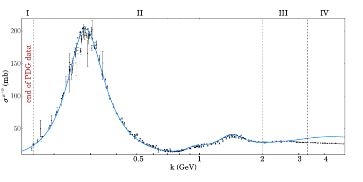
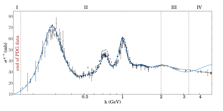
Figure 1: The SAID parameterization Workman et al. (2012) superposed on the PDG data Olive et al. (2014). This SAID solution is used only in the resonance region (region II).

In order to confront the chirally-corrected AW sum rule, Eq. (17), with experimental data in a controlled manner, it is necessary to construct a parametrization of the cross-section difference $\sigma^{-}$ of Eq. (3) over all energies. In what follows, four distinct energy regions are considered, as outlined in Table 1. The cross-section at very-low energies (region I), where there is no PDG data Olive et al. (2014), is constrained by the effective range expansion supplemented with the partial-wave expansion, while the cross-section at very-high energies (region IV) is parametrized using a Regge-model function fit to PDG $\pi p$ total cross-section data. The resonance region (region II) is parametrized by the recent SAID solution of partial wave fits to $\pi p$ scattering Workman et al. (2012) (see Fig. 1) while the transition region (region III) from the resonance region to the Regge region is constructed from an interpolation of PDG data.

		$k$ (GeV)	Source
Ia	Threshold	[0.0,0.02]	Effective Range
Ib		[0.02,0.16]	PWA Workman et al. (2012)
II	Resonance	[0.16,2.0]	SAID Workman et al. (2012)
III	Transition	(2.0,3.3)	PDG Olive et al. (2014)
IV	Regge	[3.3,$\infty$]	PDG Olive et al. (2014)

Table 1: Regions of the $\pi p$ total cross-sections. The distinguishing characteristics of these regions are the types of data available and the theoretical considerations that enter the parameterization. PDG data does not exist in region $I$. This region is further divided into $I_{a}$ where the effective range expansion is valid and $I_{b}$ where parametrizations based on partial wave analyses accurately extend.

Region I

While no experimental data exists for $\sigma^{-}$ below $k=0.16$ GeV, the total cross-section is constrained by various partial wave analyses and—within its realm of applicability—the effective range expansion, whose input parameters can be independently determined both experimentally and from Roy-Steiner-equation analyses Ditsche et al. (2012); Hoferichter et al. (2015, 2016).

As the lab-frame momentum of the pion approaches zero, the open $\pi^{0}n$ channel causes the $\pi^{-}p$ total cross-section to diverge. However, the integrated contribution in the region between the $\pi^{0}n$ and $\pi^{-}p$ threshold has been determined to be small Ericson et al. (2002); Baru et al. (2011b). Therefore, isospin invariance is assumed at $k=0$. This allows an effective range expansion of the cross-section, including the leading momentum dependence, to model the region around $k=0$. The first two terms in the effective range expansion are conventionally parametrized by combinations of isospin even and odd (upper indices $+,-$) S-wave threshold parameters. In the center-of-mass frame Höhler (1983),

$$2\sigma^{-}(q_{cm})\ =\ 8\pi\Big{[}(a_{0+}^{-})^{2}+2a_{0+}^{+}a_{0+}^{-}+\\ 2q_{cm}^{2}\left(a_{0+}^{-}b_{0+}^{-}+a_{0+}^{-}b_{0+}^{+}+a_{0+}^{+}b_{0+}^{-}+\frac{1}{24}(a_{1}^{4}-a_{3}^{4})\right)\Big{]}$$ (20)

where $q_{cm}$ is the c.m. momentum, $a_{0+}^{\pm}$ ($b_{0+}^{\pm}$) are scattering lengths (effective ranges) defined in Ref. Höhler (1983) $a_{1,3}$ are isospin $\frac{1}{2},\frac{3}{2}$ S-wave scattering lengths, and the subscripts ${\ell\pm}$ denote total angular momentum states of $j=\ell\pm\frac{1}{2}$. The relevant isovector and isoscalar scattering lengths are well known from the spectra of pionic atoms Baru et al. (2011b). In addition, recently an extraction of scattering lengths and effective ranges for the $\pi p$ system (with virtual photons removed) has been conducted using Roy-Steiner equations Hoferichter et al. (2016). Using these latter determinations, one finds (in mb)

$$2\sigma^{-}(q_{cm})=3.56(14)-2q_{cm}^{2}86(3)\ ,$$ (21)

where $q_{cm}$ is expressed in GeV. This parametrization is plotted in Fig. 2 together with the results of partial-wave analyses (PWAs) by the Jülich group Ronchen et al. (2013) and by the SAID group Workman et al. (2012). The region of applicability of the effective range expansion is less than that suggested by a naïve estimate of its radius of convergence. Figure 2 illustrates that this is due to the influence of the $P_{33}$ ($\Delta(1232)$) partial wave, which contributes even at low values of the pion momentum. Both the SAID and Jülich S-wave determinations follow the S-wave effective-range expansion throughout this region. However, the correct structure of $\sigma^{-}$ is captured only after the P-wave contributions are included. Varying the demarcation of regions I_a and I_b between $k=0.02$ GeV and $k=0.08$ GeV is treated as a means to estimate parameterization-related systematic uncertainties to the sum rule in the low-energy region.

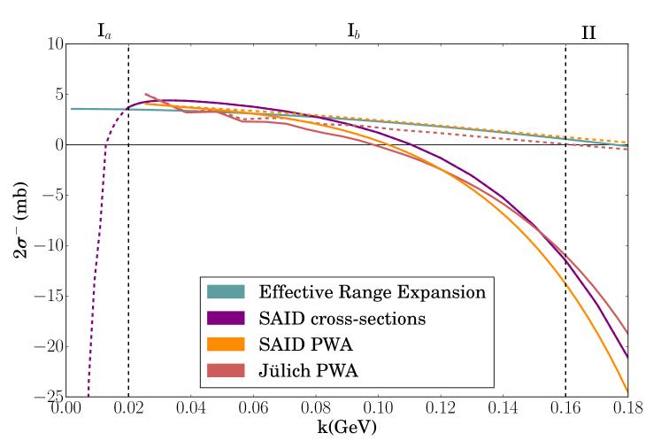
Figure 2: Parameterization of $\sigma^{-}$ in the threshold region with respect to the lab momentum, $k$, of the incoming pion. The dashed and solid lines correspond to S-wave and S,P-wave determinations of this quantity. Clearly, the P-wave is an essential contributor. The low-energy dashed region of the SAID WI08 observables solution has not been corrected for Coulomb effects and is thus replaced with the effective range expansion in this region.

Region IV

The behaviour of $\sigma^{-}$ at large momenta (Region IV) is effectively parametrized by a simple power law decay, consistent with expectations from the Regge model. This is sufficient for the purposes of this paper, and $\chi^{2}$ fitting to PDG data above $k=3.3$ GeV gives (in mb)

$$2\sigma^{-}(k)\ =\ 5.76(2)k^{-0.459(1)}\ ,$$ (22)

where again $k$ is in GeV.

Though other parametrizations of the data have been explored (see Fig. 3), the high-energy contributions to the sum rule are suppressed in the integrand, rendering differences between this simple parametrization and various other models indistinguishable. We treat these alternate fits as a means to estimate systematic uncertainties to the sum rule in the high-energy region.

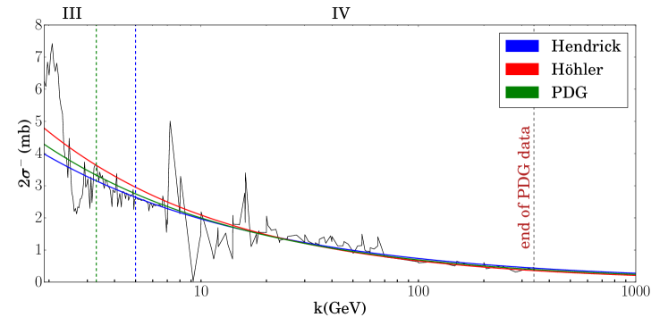
Figure 3: Three distinct (HendrickHendrick et al. (1975), HöhlerHöhler (1983) and PDGOlive et al. (2014)) power-law fits to the high-energy region of the sum rule integrand with respect to lab momentum of the incoming pion, $k$, as in Eq. (22). The dashed lines of corresponding color represent the lower-limit to the parametrization’s claimed domain of validity. The sporadic black line (ending at the right, black, dashed, vertical line) is a raw depiction of the PDG data through $\mathcal{O}(1)$ interpolation of the individual $\pi p$ cross-sections contributing to $2\sigma^{-}$ as in the decomposition of Eq. (3).

6.2 Testing the parametrization: integral moments

Given the size of the uncertainties due to the integral parametrization and the GT discrepancy, there are several sources of uncertainty that are not treated as, comparatively, they constitute fine structure: isospin violation is not considered, and uncertainties associated with interpolations of cross-section data are not treated systematically. One option in the latter case would be to implement a Gaussian process to interpolate between the $\pi^{+}$p and $\pi^{-}$p cross-section data, propagating the resulting uncertainties to $\sigma^{-}$ and to the integral of Eq. (17). Thus, the error bars quoted in this paper are a representation of expectations under reasonable variation of the dominant sources of uncertainty (neither necessarily gaussian nor defined by a definite probability to encompass the true value).

Calculating the subthreshold amplitudes through evaluation of the moment sum rules, Eqs. (15) and (16), and comparing results to other determinations establishes confidence in the parametrization of $\sigma^{-}$ developed above.

	$d_{00}^{-}\left[M_{\pi}^{-2}\right]$	$d_{10}^{-}\left[M_{\pi}^{-4}\right]$	$d_{20}^{-}\left[M_{\pi}^{-6}\right]$	$d_{30}^{-}\left[M_{\pi}^{-8}\right]$
Höhler Höhler (1983)	1.53(2)	-0.167(5)	-0.039(2)	-
$\Delta(1232)$	-0.91+1.17	-0.18	-0.04	-
Roy-Steiner Equations Hoferichter et al. (2015)	1.41(1)	-0.159(4)	-	-
This Paper	1.50(3)	-0.150(5)	-0.033(2)	-0.0075(8)
$\Delta(1232)$ $\delta$-function	1.9-1.36	-0.25	-0.046	-0.0084
S,P wave	1.9-0.77	-0.15	-0.034	-0.0089

Table 2: Calculated values of subthreshold parameters. Uncertainties represent systematic uncertainties associated with alternative parametrizations of regions I and IV and the GT discrepancy, as described in the text. Listed also are estimates of the $\Delta(1232)$-pole contributions to the moments integrals of Eq. (15) and Eq. (16). This paper has constructed two independent estimates of this contribution by (1) saturating the $\pi p$ cross-sections with a $\Delta(1232)$ $\delta$-function and (2) considering the $\pi p$ cross-sections to be constructed only of S and P partial waves. The two values stated for $d_{00}^{-}$ correspond to the $g_{\pi N}$ contribution and integral contribution to Eq. (15), respectively.

Table 2 displays the subthreshold parameters as calculated from (i) the work of Höhler Höhler (1983) (ii) a recent analysis of the $\pi p$ amplitude with Roy-Steiner (RS) equations Hoferichter et al. (2016), and (iii) the moment sum rules using the cross-section parameterization of Section 6.1. The uncertainty estimate of $d_{00}^{-}$ is dominated by the uncertainty in the value of $g_{\pi N}$ stemming from the GT discrepancy. This explains the order of magnitude larger uncertainties as compared to the higher moments. To construct this estimate, we have used the 2% upper limit expected on the GT discrepancy as discussed in Ref. Hoferichter et al. (2010). Contributions to the uncertainty arising from alternative Regge fits or from modifying the threshold values of the effective-range parameters are comparatively insignificant, although they are incorporated into the table above.

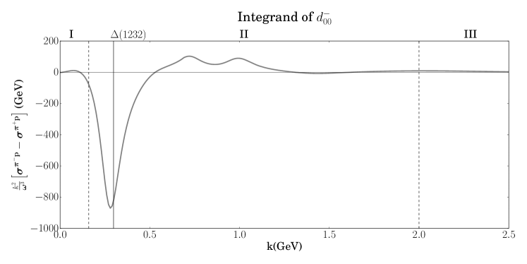
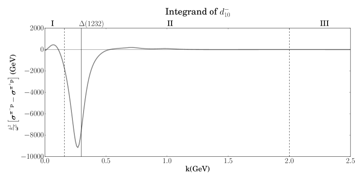
Figure 4: Integrands expressed in the integration variable $k$ associated with the first two subthreshold coefficients. Note that $k$ is not the variable chosen to express these coefficients in Eqs. (15) and (16). Thus, the solid vertical line is placed at the $\Delta(1232)$ contribution as a pertinent reference. For higher moments, the integrand tends to increase the influence of the threshold region as well as the influence of the $\Delta(1232)$ relative to higher $\Delta$ and $N$ resonances. This is consistent with the numerical findings that the value of subthreshold parameters in Table 2 are closely approximated when considering only the $\Delta(1232)$ resonance.

The higher moments are only sensitive to the cross-section very near threshold and the $\Delta(1232)$ peak. Evidently, several of the coefficients are effectively saturated by the $\Delta(1232)$ resonance contribution to the sum rule. These observations are illustrated in Figure 4 as well as in Table 2, where saturation with the $P_{33}$ partial wave results in a 3% difference for $d_{20}^{-}$ and even less for $d_{10}^{-}$. These statements are based on replacing the full PWA of the resonance region with S and P partial waves only. Saturation of the integrand with a $\delta$-function constructed from PDG values for the $\Delta(1232)$ resonance leads to similar agreement and will be discussed in greater detail in Section 6.3 and 6.4 where, for comparison with the full continuous parameterization, the integrand is saturated with N and $\Delta$ resonances of three and four star PDG significance. It is reasonable to conclude that beyond these two coefficients, $d_{00}^{-}$ and $d_{10}^{-}$, even the dominant peak of the $\Delta$ begins to lose its significance in light of the increased weighting of the threshold region.

We stress that the goal of this section is not to achieve precision but rather to test the parametrization of the cross-section for consistency against existing data and theoretical constraints. It is encouraging that the values of the subthreshold parameters found here from the moment sum rules are comparable to those found from independent sources. The combination of these internal and external consistencies is taken as license to make use of the parameterization of Section 6.1 in evaluating the $\mathcal{O}(M_{\pi}^{3})$ corrected AW sum rule for $g_{\scriptscriptstyle A}$.

6.3 Results: the axial-vector coupling constant

Eq. (18)	$g_{A}\,\mathcal{O}(M_{\pi}^{2})$	$\Delta_{AW}$	%
Höhler	1.282(12)	0.28(3)	21.8
Roy Equations	1.242(10)	0.18(3)	14.5
This Paper	1.272(15)	0.257(36)	20.2
Eq. (19)	$g_{A}\,\mathcal{O}(M_{\pi}^{2})$	$\Delta_{AW}$	%
Roy Equations	1.255(10)	0.21(2)	16.7

Table 3: Calculations of the axial-vector coupling constant and AW discrepancy (Eq. (17)) using the subthreshold coefficients of Table 2. Uncertainties, as discussed in the text, are estimated from the parameterization, the GT discrepancy (7), and the truncation of the AW discrepancy beyond $\mathcal{O}\left(M_{\pi}^{3}\right)$. The third column corresponds to the relative contribution of the AW discrepancy to calculations of $g_{A}$ at this order in $\chi$PT.

With a controlled parameterization of the total cross-section over all energies in hand, the AW sum rule can now be used to determine $g_{\scriptscriptstyle A}$. Note that $g_{\scriptscriptstyle A}$ appears within the value of the AW discrepancy itself (see Eq. (18)). Hence, one can treat the AW sum rule as a non-linear equation for $g_{A}$, and then use this calculated value to determine the contribution from $\Delta_{AW}$. Having done this with the current parameterization and coefficients from Roy-Steiner equations leads to the value: $g_{\scriptscriptstyle A}=1.248\pm 0.010\pm\ 0.007\pm 0.013$, where uncertainties are from the parametrization of the integral in the sum rule, the GT discrepancy, and the truncation of the chiral expansion. Table 3 presents the results of this calculation from Eq. (18) with alternate sets of subthreshold parameters detailed in Table 2 and Eq. (19) using the LECs of Ref. Hoferichter et al. (2015). The distribution of uncertainties for these estimates are comparable to that stated above. In what follows, we will discuss the sources of uncertainty in some detail.

The non-linear equation for $g_{A}$ was solved using gaussian-approximated, correlated uncertainties for $\bar{d}_{1}+\bar{d_{2}}$, $\bar{d}_{5}$, $c_{1}$, $c_{3}$, and $c_{4}$ as well as uncorrelated uncertainties for $d_{00}^{-}$, $\bar{d}_{18}$, and the 2012 PDG value of $F_{\pi}$. These sources of uncertainty are associated with specific parameterization choices and the GT discrepancy (2% as discussed in Ref. Hoferichter et al. (2010)), and are represented by the first two numbers of the quoted, partitioned uncertainty for $g_{A}$. For the third source of uncertainty, we considered the truncation of $\Delta_{AW}$ at $\mathcal{O}\left(M_{\pi}^{3}\right)$. Note that estimating the truncation uncertainty from, for instance, a number of order unity times $\left({M_{\pi}}/{4\pi F_{\pi}}\right)^{4}$, leads to uncertainties much smaller than those that are quoted. Instead, the uncertainty due to truncation is estimated by the consistency of the analysis in the event that one returns to the dispersion relation, Eq. (13), and derives a new AW discrepancy. The alternate expansion that we considered occurs when the pion-mass dependence of the lab momentum, $k$, appearing in the sum rule integrand is also expanded in powers of $M_{\pi}$. While this no longer arrives at a correction to the chiral-limit AW sum rule, this resummation allows for an estimate of the influence of neglected higher order terms. Using this method leads to an estimated truncation uncertainty slightly larger than that implied by naive dimensional analysis. Included also in this estimate of the truncation error is the higher-order difference between Eq. (18) and Eq. (19). Together, the three dominant sources of uncertainty combine to yield the overall uncertainty stated in Table 3.

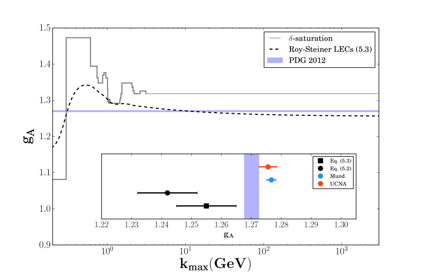
Figure 5: Calculated value of $g_{\scriptscriptstyle A}$ with increasing upper bound of the integrated total cross-section within the AW sum rule, Eq. (17). Results in the main plot are from the evaluation of Eq. (19) with the LEC values of Ref. Hoferichter et al. (2015). The subplot includes the corresponding evaluation with Eq. (18) as well as two recent measurements of $g_{\scriptscriptstyle A}$ from neutron $\beta$-decay Mund et al. (2013); Mendenhall et al. (2013) for comparison. The light gray line represents a similar analysis with the total cross-section saturated by $\delta$-function resonances Beane and van Kolck (2005) and this paper’s evaluation of subthreshold parameters. The light-blue band is the 2012 PDG value for $g_{\scriptscriptstyle A}$.

Focusing on the independent evaluations which rely on recent Roy-Steiner calculations of $d_{00}^{-}$ and the correlated LECs, one finds that the two $\mathcal{O}(M_{\pi}^{3})$ evaluations of $g_{\scriptscriptstyle A}$ are internally consistent. More importantly, one finds that the magnitude and sign of $\Delta_{AW}$ are in agreement with the experimental observation that the value of $g_{\scriptscriptstyle A}$ is approximately 25% larger than its chiral limit value. In the next section, we will examine this symmetry breaking in greater detail.

6.4 The physical picture

The AW sum rule is a constraint on the flow of null-plane, axial-vector charge between the nucleon and all other states that the nucleon can transition to through the emission or absorption of a pion. The transitions can occur only because the charges are not conserved (they depend on $x^{+}$) and therefore they are able to mediate the energy transfer that is necessary for the processes to take place. Of course, physically, the non-conservation of the null-plane axial-vector charge signals spontaneous chiral symmetry breaking. This picture is, strictly speaking, correct only in the chiral limit and therefore in this case the deviations of $g_{\scriptscriptstyle A}$ from unity are a measure of spontaneous symmetry breaking. As we have seen here, $\chi$PT allows the quantitative inclusion of corrections to this picture due to non-vanishing light-quark masses via $\Delta_{AW}$. An intuitive visual representation of the sum rule gives the value of $g_{\scriptscriptstyle A}$ as a function of the upper value of the integration momentum ($k_{\text{max}}$) as it is increased from zero to its asymptotic value. (See Figure 5.) As one sees in the plot, methodically adding states of higher energy under the integral (increasing $k_{\text{max}}$) adds and subtracts chiral charge, depending on the intermediate state.

When the chiral-limit sum rule (Eq. (11)) is expressed in terms of physical quantities to produce the leading, $\mathcal{O}(M_{\pi}^{0})$ contribution (Eq. (12)), the axial-vector coupling constant at $k_{max}=M_{\pi}$ is exactly 1. With the introduction of chiral corrections, this value is shifted to $1+\Delta_{AW}$. Once the chiral symmetry is spontaneously broken, intermediate states that transition to the nucleon via the non-conserved axial-vector charge can and do appear. In the interest of gaining understanding of the weightings associated with these states, depicted by the evolution of the integral in Figure 5, the integrand can be modeled with a finite number of known resonances which couple strongly to the pion-nucleon system. This process, $\delta$-saturation, was carried out in Ref. Beane and van Kolck (2005), where the cross-sections participating in the AW sum rule were approximated by $\delta$-functions of the appropriate N and $\Delta$ resonances using the chiral-limit form of the sum rule. Here, this exercise is repeated, but including the effect of the AW discrepancy. Figure 5 shows that the delta functions lead to a series of step functions in the calculation of $g_{A}$ that, as expected, qualitatively track the curvature of the actual integrand obtained from the parameterization of cross-sections.

While the $\delta$-saturation of Ref. Beane and van Kolck (2005) neglected the AW discrepancy, the analysis resulted in an evaluation of $g_{A}\simeq 1.26$—a value surprisingly close to experiment, albeit with no measure of uncertainty. Saturating the AW sum rule using the same set of resonances but with Breit-Wigner line shapes and a threshold region as discussed in Section 6.1 yields the value $g_{\scriptscriptstyle A}\simeq 1.27$ (with $\Delta_{AW}=0$). With the now-improved understanding of the chiral corrections to the AW sum rule, these past successes of $\delta$-saturated models may seem more fortuitous than illuminating. However, both this “leading-order” agreement and the qualitative agreement of Figure 5 indicates that models of pion-nucleon scattering, and more generally of the nucleon null-plane wave-function, that implement a finite number of resonances, provide an approximate description that could prove useful for modeling the internal axial structure of the nucleon.

The subplot of Figure 5, provides a comparison between sum rule determinations of $g_{\scriptscriptstyle A}$ and current experimental measurements of the coupling constant. According to the 2012 PDG review, $g_{\scriptscriptstyle A}=1.2701(25)$. Recent experimental measurements of the neutron $\beta$-decay asymmetry parameter gives $g_{\scriptscriptstyle A}=1.276(3)$ Mund et al. (2013)Mendenhall et al. (2013). While the uncertainties that arise in the AW sum rule determination of $g_{\scriptscriptstyle A}$ presented in this paper are not particularly aggressive (claiming high precision), the results bring the sum-rule determination of $g_{\scriptscriptstyle A}$ into consistency with current measured values of $g_{\scriptscriptstyle A}$ and emphasize the physical mechanism of QCD that is responsible for the axial-vector charge’s deviation from unity.

7 Conclusions

The AW sum rule is a unique signature of chiral symmetry and its breaking in QCD as its validity resides in both the algebraic content of chiral symmetry, which guarantees the convergence of the sum rule, and the dynamical content of chiral symmetry, which allows the systematic inclusion of light-quark mass effects. In this paper, it has been shown how, using results of $\chi$PT, the chiral limit sum rule may be systematically extended to include corrections up to $\mathcal{O}(M_{\pi}^{3})$. In addition, the introduction of the AW discrepancy allows a non-unique but useful means of separating the contributions to the deviation of $g_{\scriptscriptstyle A}$ from unity into distinct parts that arise from spontaneous and explicit chiral symmetry breaking.

While the calculation presented here is, by construction, independent of experimental measurements of $g_{\scriptscriptstyle A}$, the parameterization we have established may be useful beyond the determinations of $\Delta_{AW}$ and $g_{\scriptscriptstyle A}$ provided here. Considering the current precision of $g_{\scriptscriptstyle A}$ measurements, it is reasonable to consider rearranging the $\mathcal{O}(M_{\pi}^{3})$ sum rule to take the value of $g_{\scriptscriptstyle A}$ as experimental input for a determination of LECs. For example, recall that $\Delta_{AW}$ may be expressed in terms of a linear combination of LECs of the $\pi p$ system (Eq. (19)). Thus, $g_{\scriptscriptstyle A}$ is a physical quantity with direct dependence on the LEC correlation matrix—a now essential piece of any LEC extraction. Similarly, the AW sum rule may be used to constrain the LEC $\bar{d}_{18}$, which parametrizes the GT discrepancy, a significant source of uncertainty in many calculations, including those of $g_{\pi N}$. Whether the AW sum rule (with the correction of $\Delta_{AW}$) will provide significant constraints on such LECs will be left as a question for future research.