Detecting fast radio bursts at decametric wavelengths

Abstract

Fast radio bursts (FRBs) are highly dispersed, sporadic radio pulses that are likely extragalactic in nature. Here we investigate the constraints on the source population from surveys carried out at frequencies $<1$ GHz. All but one FRB has so far been discovered in the 1–2 GHz band, but new and emerging instruments look set to become valuable probes of the FRB population at sub-GHz frequencies in the near future. In this paper, we consider the impacts of free-free absorption and multi-path scattering in our analysis via a number of different assumptions about the intervening medium. We consider previous low frequency surveys alongwith an ongoing survey with the University of Technology digital backend for the Molonglo Observatory Synthesis Telescope (UTMOST) as well as future observations with the Canadian Hydrogen Intensity Mapping Experiment (CHIME) and the Hydrogen Intensity and Real-Time Analysis Experiment (HIRAX). We predict that CHIME and HIRAX will be able to observe $\sim$ 30 or more FRBs per day, even in the most extreme scenarios where free-free absorption and scattering can significantly impact the fluxes below 1 GHz. We also show that UTMOST will detect 1–2 FRBs per month of observations. For CHIME and HIRAX, the detection rates also depend greatly on the assumed FRB distance scale. Some of the models we investigated predict an increase in the FRB flux as a function of redshift at low frequencies. If FRBs are truly cosmological sources, this effect may impact future surveys in this band, particularly if the FRB population traces the cosmic star formation rate.

1 Introduction

The origin of fast radio bursts (FRBs) remains an unanswered question since their discovery a decade ago (Lorimer et al., 2007). FRBs are millisecond duration, highly sporadic and dispersed radio pulses which follow the same dispersion relation seen in radio pulses from neutron stars. Of the 20 FRBs known so far, 18 have been found at Parkes (Thornton et al., 2013; Lorimer et al., 2007; Petroff et al., 2015; Keane et al., 2016; Champion et al., 2016), one at Arecibo (Spitler et al., 2014, 2016) and one at Green Bank (Masui et al., 2015). With the exception of the latter, FRB 110523, which was detected at 800 MHz, all the other FRBs have so far been seen in the 1–2 GHz band. FRB dispersion measures (DMs) are substantially greater than that expected from free electrons in our Galaxy, suggesting that FRBs are extragalactic in origin. There have been arguments about local origin of FRBs but the models cannot explain all the observed characteristics (for a review, see Katz, 2016).

Broadly speaking, the FRB source models fall into two categories: those of a catastrophic nature which would only be seen once (e.g., prompt emission from a gamma-ray burst; Yamasaki et al., 2016) or those with the possibility to repeat (e.g., giant pulses from Crab-like pulsars; Cordes & Wasserman, 2016; Cordes et al., 2004). So far, the only source known to repeat is FRB 121102 (Spitler et al., 2016). In the light of these recent discoveries, and to try to shed light on the origins of FRBs a number of groups are carrying out extensive radio surveys at sub-GHz frequencies (Karastergiou et al., 2015; Caleb et al., 2016; Deneva et al., 2016). To date, however, the 0.7–0.9 GHz detection of FRB 110523 remains the only source found below 1 GHz (Masui et al., 2015).

Lyutikov et al. (2016) argues that a lack of detections could be due to absorption in an ionized medium along the line of sight. Recent discoveries suggest low scattering in all FRBs which precludes a local plasma in the vicinity of the progenitor to explain their high DMs (Masui et al., 2015; Macquart & Koay, 2013). Kulkarni et al. (2015) argue for a young magnetar model with circum-dense medium around the star which can explain the high DM and the non-detections at lower frequency due to free-free absorption. The non-detections can also be explained by young neutron star progenitor within an expanding supernova remnant shell with hot ionized filaments (Piro, 2016).

In this paper, we present a detailed analysis of the aforementioned absorption and scattering models. We use the approach to investigate the significance of non-detections in three recently completed surveys to constrain the spectral index of the burst for each model. Based on these constraints we make predictions for FRB detections from CHIME, UTMOST and HIRAX. Connor et al. (2016) make optimistic predictions for these upcoming low frequency surveys based on single FRB detection in the 0.7–0.9 GHz band. Here, we present predictions on the FRB detection rates based on different models of flux mitigation in the ISM. The plan for this rest of this paper is as follows. We describe our analysis methods in §2. In §3, we describe our results and discuss their implications in §4.

2 Methods

This section describes the methodology used for obtaining upper limits on FRB predictions with CHIME under different astrophysical scenarios. Our study is motivated by our recent work on modeling gigahertz peaked spectrum pulsars via free-free absorption (Rajwade et al., 2016). Here, we investigate what could happen to an FRB that is absorbed or scattered and how that affects detectability with CHIME and UTMOST. We will begin by making use of the recent null results of FRB detections in the ongoing UTMOST survey (Caleb et al., 2016), the Arecibo drift scan survey (AO327; Deneva et al., 2016) and the 145 MHz LOFAR survey (Karastergiou et al., 2015). We also considered the 155 and 182 MHz surveys with the Murchison Widefield Array (MWA) (Tingay et al., 2015; Rowlinson et al., 2016) in our analysis. However, since the flux limits for those surveys are higher than the LOFAR survey, the spectral index constraints are less stringent than the LOFAR survey. We do not include results from single-pulse searches in the ongoing Green Bank North Celestial Cap (GBNCC) survey (Stovall et al., 2014) in this analysis. A paper describing the constraints from these results will be presented elsewhere (Chawla et al., in prep).

2.1 Flux–redshift relationship and baseline model

Our methodology builds upon that used by Karastergiou et al. (2015) in their LOFAR survey, to include the effects of free-free absorption and scattering. Following these authors, we assume that FRBs are standard candles and the energy output from the source follows a power law with respect to frequency (see, e.g., Lorimer et al., 2013). Then, the peak flux density

$$S_{\rm peak}=\frac{L~{}\int_{\nu_{1}(1+z)}^{\nu_{2}(1+z)}E_{\nu^{\prime}}d\nu^{\prime}}{4\pi D(z)^{2}~{}\left(\nu_{2}-\nu_{1}\right)~{}\int_{\nu^{\prime}_{\rm low}}^{\nu^{\prime}_{\rm high}}E_{\nu^{\prime}}d\nu^{\prime}},$$ (1)

where $L$ is the bolometric luminosity, the pulse energy $E_{\nu^{\prime}}\propto\nu^{\prime\alpha}$ for some spectral index $\alpha$ and source frame frequency $\nu^{\prime}=(1+z)\nu$ at redshift $z$ and luminosity distance $D(z)$. Also in the source frame, $\nu^{\prime}_{\rm low}$ and $\nu^{\prime}_{\rm high}$ are the frequency bounds in which the source emits. Following Lorimer et al. (2013), we assumed $\nu^{\prime}_{\rm high}=$10 GHz and $\nu^{\prime}_{\rm low}=$10 MHz. The observed frequency band is defined by $\nu_{1}$ and $\nu_{2}$ and is different for each survey under consideration. We will discuss the implications of this standard-candle assumption in §4.3.

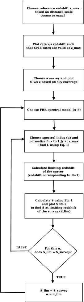
Figure 1: Flow diagram showing the logical flow of our analysis procedure for placing constraints on the spectral index. For further details, see §2.1.

Our implementation of the earlier study by Karastergiou et al. (2015) to place constraints on FRB spectral indices is summarized in Fig. 1 and described below. Since the distance scale for FRBs is not well known, we consider two scenarios: (i) a “cosmological model” for which the maximum redshift $z_{\rm max}=0.75$ (see, e.g., Lorimer et al., 2013); (ii) an “extragalactic model” for which the characteristic distance is 100 Mpc (i.e. $z_{\rm max}=0.025$; see, e.g. Lyutikov et al. 2016). Having chosen one of these two scales, we then derive the FRB rate versus redshift relationship by assuming an FRB population with constant density per unit comoving volume out to $z_{\rm max}$. At the chosen value of $z_{\rm max}$ this rate matches, by definition, the rates published by Crawford et al. (2016) based on FRB surveys at Parkes. Using this curve, for each of the other surveys under consideration (i.e. LOFAR, AO327 and UTMOST), we can compute the number of FRBs expected as a function of redshift by multiplying the rate–redshift relationship by the appropriate survey sky and time coverage. The resulting number versus redshift curves then lead to a limiting redshift $z_{\rm lim}$ for each survey. This limiting redshift is defined to be that at which $<1$ FRB is predicted to be seen in each survey. An example of one such calculation is shown for UTMOST in the left panel of Fig. 2.

Next, for each of the source models A–F described in detail below, we choose a spectral index $\alpha$ and, using Eq. 1, find the corresponding value of $L$ such that $S_{\rm peak}=1$ Jy at $z_{\rm max}$. The 1 Jy reference flux is approximate, and motivated by the results of Thornton et al. (2013). Our results turn out to be insensitive to the exact value adopted here. For each of the surveys under consideration, we calculate the corresponding flux at the survey’s redshift limit, i.e. $S_{\rm peak}(z_{\rm lim})$ and iterate until the spectral index is found where $S_{\rm peak}(z_{\rm lim})$ equals the survey flux limit. This spectral index is, by definition, the limiting value appropriate to the assumptions of that particular model and distance scale, and we refer to this lower limit as $\alpha_{\rm lim}$.

Our baseline model, which follows this process using a simple power-law spectral behaviour amounts to a repeat of the analysis of Karastergiou et al. (2015). We refer to this case as model “A” henceforth and, as necessary, distinguish between the cosmological and extragalactic cases in the text. The relevant parameters used for each of these models and constraints obtained from them are given in Table 2 and discussed further in the sections below.

2.2 FRB survey sensitivity model

From radiometer noise considerations, if $W$ is the width of the FRB then, for a search in which the pulse is optimally match filtered by a top-hat pulse of peak flux density $S$, the signal-to-noise ratio

$${\rm S/N}=\frac{S\,G\sqrt{Wn_{\rm p}\Delta\nu}}{T_{\rm sys}},$$ (2)

where $T_{\rm sys}$ is the system temperature, $\Delta\nu$ is the bandwidth, $n_{\rm p}$ is the number of polarizations summed and $G$ is the gain. In all current FRB surveys, where incoherent dedispersion techniques are used to process the data, and in the context of our models DM depends on redshift, then there is a dispersive broadening effect that results in a dependence between survey sensitivity and redshift. To model this effect, we compute the effective width of the pulse

$$W_{\rm eff}=\sqrt{W_{\rm int}^{2}+W_{\rm DM}^{2}+W_{\tau}^{2}},$$ (3)

where $W_{\rm int}$ is the intrinsic pulse width of the FRB, $W_{\rm DM}$ is the intra-channel dispersion smear and $W_{\tau}$ is the additional broadening due to the finite sampling interval of the survey. To calculate $W_{\rm DM}$, we adopted a DM-redshift scaling from (Inoue, 2004) where DM $=1200~{}z$ cm^-3 pc. Using the standard expression for dispersion broadening (see, e.g., Lorimer & Kramer, 2004), we have

$$W_{\rm DM}=99.6\,{\rm ms}\left(\frac{z}{n_{\rm chan}}\right)\left(\frac{\Delta\nu}{\rm MHz}\right)\left(\frac{\nu}{\rm GHz}\right)^{-3},$$ (4)

where $n_{\rm chan}$ is the number of frequency channels used for dedispersion. Future FRB surveys may well introduce high-speed algorithms to implement coherent dedispersion (see, e.g. Zackay & Ofek, 2014), in which case $W_{\rm DM}$ will not be necessary. To model the degradation due to incoherent dedispersion of current and near-future surveys, consider an “optimal survey” signal-to-noise ratio, S/N₀ which is obtained from Eq. 2 for the case for a top-hat pulse with height $S_{0}$ and width $W_{\rm int}$. For a broadened pulse of width $W_{\rm eff}$, energy conservation means that its peak flux density is $S_{0}W_{\rm int}/W_{\rm eff}$. It is straightforward to show that the S/N of the broadened pulse is lower than S/N₀ by a factor of $\sqrt{W_{\rm int}/W_{\rm eff}}$. For an actual survey with a constant S/N threshold, this amounts to an increase in the limiting peak flux density for detection by the reciprocal of this factor, so that the resulting limiting sensitivity

$$S_{\rm lim}=S_{0}\sqrt{\frac{W_{\rm eff}}{{W_{\rm int}}}}=\frac{{\rm S/N}_{\rm lim}\,T_{\rm sys}}{G\,W_{\rm int}}\sqrt{\frac{W_{\rm eff}}{n_{p}\Delta\nu}}.$$ (5)

This expression is used when calculating the sensitivity curves throughout this paper (see, e.g., the right panel of Fig. 2). Here S/N_lim is the limiting signal-to-noise ratio required for a detection in a given survey. Table 1 summarizes the essential observing parameters for each of the surveys considered in this paper.

Survey	Centre frequency	Bandwidth	Flux limit	Reference
	(MHz)	(MHz)	mJy
UTMOST	843	31.5	11000	Caleb et al. (2016)
AO327	327	57	83	Deneva et al. (2016)
LOFAR	145	6	62000	Karastergiou et al. (2015)
CHIME	600	400	125	Newburgh et al. (2014)
HIRAX	600	400	24	Newburgh et al. (2016)

Table 1: Table showing various parameters of different surveys. The system parameters of CHIME and HIRAX are estimated values (see text for details).

3 Models for flux mitigation

Radio signals propagating through the ISM are modulated by free electrons in the intervening medium. These interactions leave observational signatures in the received radiation at the earth. Some of these signatures (e.g. scattering, free-free absorption and scintillation) have been observed in various radio sources. FRBs, being astrophysical in nature, are subject to the same phenomena. It is therefore important to model these effects in detail before we draw any inferences about their intrinsic spectral indices and make predictions for future surveys. Below, we describe our mathematical models to characterize effects of scattering and free-free absorption.

3.1 Models including free-free absorption

As discussed by other authors (Kulkarni et al., 2015; Lyutikov et al., 2016), but not taken into account by Karastergiou et al. (2015), thermal absorption can significantly reduce FRB fluxes at lower frequencies. For this analysis, following our earlier work (Rajwade et al., 2016), we assume

$$E_{\nu^{\prime}}\propto\nu^{\prime\alpha}~{}{\rm exp}\left(-\tau\nu^{\prime-2.1}\right),$$ (6)

where, as described further by Rajwade et al. (2016), the optical depth of the absorber

$$\tau=0.082~{}T_{e}^{-1.35}~{}{\rm EM}.$$ (7)

Here $T_{e}$ is the electron temperature and EM is the emission measure of the absorber. Then the peak flux is computed by combining Eq. 1 and Eq. 6. We consider two cases for absorption: (i) cold, molecular clouds with ionization fronts for which $T_{e}=200$ K and EM $=1000$ cm^-6 (Lewandowski et al., 2015) (hereafter, model B); (ii) hot, ionized magnetar ejecta/circum-burst medium for which $T_{e}=8000$ K and EM $=1.5\times 10^{6}$ cm^-6 (hereafter, model C). The value of EM for model C has been chosen from a range of values reported in Rajwade et al. (2016), Kulkarni et al. (2015) and Lewandowski et al. (2015).

Model	$T_{e}$	EM		$\alpha_{\rm lim}$					$z_{\rm lim}$
	(K)	cm-6pc	UTMOST		LOFAR		AO327		CHIME
			cosmo	exgal	cosmo	exgal	cosmo	exgal	cosmo	exgal
A	—	—	–0.70	–1.30	0.0	–0.50	0.70	1.25	1.54	0.10
B	200	1000	–0.80	–1.30	–1.0	–2.10	0.50	1.10	1.56	0.10
C	8000	$1.5\times 10^{6}$	–1.50	–2.50	—	—	–0.30	–2.85	1.64	0.09
D	—	—	–2.10	–3.30	–3.0	–4.0	–3.30	–2.20	0.84	0.06
E	200	1000	–2.20	–3.30	–4.10	–5.70	–3.50	–2.50	0.85	0.06
F	8000	1.5$\times$106	–2.70	–4.50	—	—	–4.50	–6.45	0.82	0.05

Table 2: Model parameters and resulting spectral constraints from the various surveys considered. From left to right, we list the model, assumed electron temperature ($T_{e}$) and emission measure (EM), limiting spectral index ($\alpha_{\rm lim}$) for the three published surveys (LOFAR, AO327 and UTMOST). For the future CHIME survey, we list the limiting redshift ($z_{\rm lim}$) predicted by our models. The “cosmo” and “exgal” columns give results from the two different distance scales assumed: “cosmological” ($z=0.75$) and “extragalactic” ($z=0.025$) as defined further in the text.

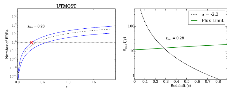
Figure 2: Left: Number of FRBs versus redshift for the UTMOST survey parameters Caleb et al. (2016). The curves indicate the Crawford et al. (2016) rates with 99$\%$ bounds. The horizontal line corresponds to one FRB. The intersection of the horizontal line and the upper bound of the curve is shown by the red cross at $z=0.28$. Right: peak flux versus redshift for UTMOST survey for model E (dashed curve). The solid line shows the flux limit of the UTMOST survey. The intersection of the two curves is denoted by z_lim. Note the non-linear dependence of flux limit with redshift for both surveys shown here is due to the impact on intra-channel dispersion broadening upon sensitivity (see §2.2 for details).

3.2 Models including multi-path scattering

Multi-path scattering due to free electrons in the ionized medium along the line of sight to the observer can cause a reduction in the measured flux at the telescope. Scattering manifests itself as an exponential tail in the radio pulse of the FRB. FRBs that have been discovered so far, show only a modest amount of scattering: for the 17 FRBs, 10 of them have scattering measurements and 7 have them have upper limits (Cordes et al., 2016). Hence, we computed the scattering timescale by taking the average of the published values (estimates and upper limits) of these 17 sources. For sources with upper limits, conservatively, we assumed those values as measured values when taking the average. We obtained a mean scattering timescale of $\sim$8.1 ms at 1 GHz. We note that if we assume the scattering timescales for sources with upper limits as half of the upper limit values, we get a average timescale of $\sim$6.7 ms which is also a high value. Using the most conservative value, the scattering timescale $\tau_{s}$ can be computed for any frequency $\nu$ via the $\nu^{-4}$ scaling law (Bhat et al., 2004) as opposed to $\nu^{-4.4}$. The non-Kolmogorov scaling exponent is due to fact that the diffraction length scale is smaller than the inner scale of the wavenumber spectrum (see Bhat et al., 2004, , and references therein). Assuming that energy of the burst is conserved, if the pulse scatters with a timescale of $\tau_{s}$, the width increases and hence, the measured flux reduces by a factor of $\sqrt{1+(\tau_{s}/W_{\rm eff})^{2}}$ where $W_{\rm eff}$ is the effective pulse width defined in the preceding section. Including this effect into our analysis, we introduce three final models. Model D has scattering with no free-free absorption, while models E and F have scattering in addition to the respective absorption parameters adopted for models B and C.

4 Results

4.1 Spectral index constraints

Taking into account all the factors discussed in the previous section, the results of our analysis are collected for models A–F in in Table 2. For each of these models, we constrained the spectral indices assuming each of the two distance constraints in turn. A graphical illustration of this process is shown for model E as an example in Fig. 2 where we show the constrained spectral index for one of the models for the UTMOST survey (Caleb et al., 2016). As mentioned previously, our baseline model (A) is an update on the results of Karastergiou et al. (2015) using the more recent rate FRB rate estimates from Crawford et al. (2016). In our analysis, which also includes the non-detections in UTMOST and AO327, the most constraining power-law spectral index for this model is $\alpha>0.7$ for the cosmological distance scale from AO327. The most constraining spectral index ($\alpha>1.25$) is obtained from the AO327 survey if the extragalactic distance scale is applied to this survey.

In model B, where we go beyond the simple power-law spectral dependence and include free-free absorption with cold molecular clouds, we find only a modest change in the results for model A for AO327 and UTMOST but as expected a greater deviation at the LOFAR frequency band where spectral turnover effects are more severe. The LOFAR survey does not in fact provide any constraints on the spectral index for models C and F, where a hot ionized medium is assumed. These models predict flux densities below the survey threshold for essentially all values of $\alpha>-10$. The corresponding $\alpha_{\rm lim}$ values are therefore not listed in Table 2.

The spectral index constraints become much weaker when the effects of interstellar scattering are incorporated in models D, E and F. For model D, with scattering but no free-free absorption is assumed, the UTMOST null results only bound $\alpha>-2.2$ for the cosmological case and the AO327 results bound $\alpha>-2.2$ for the extragalactic case. When free-free absorption and scattering are considered in models E and F, these constraints are diminished further.

4.2 FRB rate predictions for future surveys

Fig 3 shows the predicted detection rates for UTMOST, CHIME and HIRAX for the two distance scales considered. The vertical line corresponds to the redshift limit of the survey for all models A–F. These predictions were obtained from the spectral constraints on each model obtained in the previous section, and computing the sensitivity of each survey as described below.

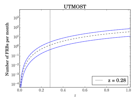
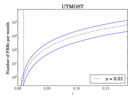
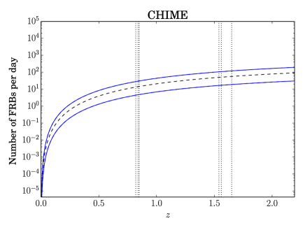
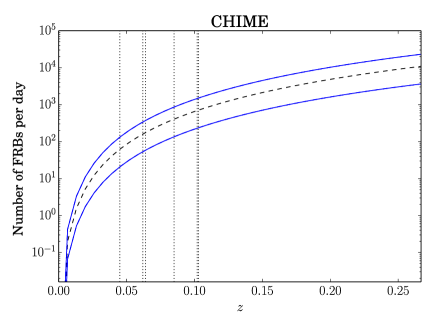
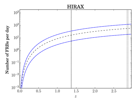
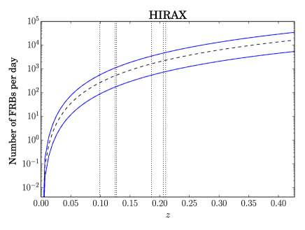
Figure 3: The number of FRBs predicted per day/month as a function of redshift for various surveys. The black dashed curve is the number of FRBs per day based on the  (Crawford et al., 2016) rates. The blue curves are the 99$\%$ upper and lower bounds on the black dashed curve. Left panels show predictions for the cosmological case while the right panels show predictions for extragalactic case. In predictions for CHIME (cosmological case), from left to right, the vertical lines correspond to models F,D,E,A,B and C respectively while they correspond to models F,E,D,C,B and A respectively for the extragalactic case. Similarly for HIRAX, the vertical lines from left to right correspond to models D,E,F,A,B and C respectively for the cosmological case and F,E,D,C,B and A respectively for the extragalactic case. In case of UTMOST, the single vertical line corresponds to all models for their respective constrained spectral index at the limiting redshift of the survey. The ordinate of intersection of the vertical line and the curves gives the predicted number for each model.

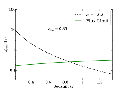
Figure 4: Peak flux versus redshift predicted for model E assuming the nominal parameters of CHIME. The intersection of the survey limit and the curve gives the limiting redshift probed by CHIME for this model.

In modeling the sensitivity of CHIME, we assume that the gain $G=2$ K Jy^-1 and system temperature $T_{\rm sys}=50$ K remain constant over the band. We also assumed a single CHIME beam of width 1.5 by 90 degrees (Bandura, private communication). Using Eq 2, we obtained the optimum flux limit of 0.125 Jy for a 5 ms duration burst. For the scattering scenario, we used the frequency weighted average value of $\tau_{s}$ over the whole CHIME band. We obtained $\tau_{s}=$ 92.2 ms. For each of the models described in Table. 2, and the using the constraint on the spectral index from the UTMOST survey, we plotted the peak flux versus redshift using Eq. 2. For each model at the constrained spectral index, we obtained the $z_{\rm lim}$ which is the redshift where the peak flux of the FRB is equal to the flux sensitivity limit of CHIME as shown in Fig. 4. Then, using the expected sky coverage of CHIME and scaling the Crawford et al. (2016) rate with the comoving volume, we obtained the predicted number of FRB detections per day versus redshift as shown in left panel of Fig. 3. The ordinate of the point at which the $z_{\rm lim}$ for each model intersects the curve and the bounds gives the predicted number of FRB detections per day for that given model. We investigated the yield for HIRAX surveys with identical parameters as the ones used for CHIME except for $G$ = 10.5 K Jy^-1. The analysis suggests that CHIME will be able to detect from 30–100 FRBs per day depending on the model for the cosmological case while the yield increases by an order of magnitude ($\sim$150–1000 FRBs per day) for the extragalactic case due to the sharp dependence of rates with redshift. Similarly, HIRAX will be able to detect 50–100 FRBs per day for the cosmological case and 700–4000 FRBs per day for the extragalactic case.

4.3 Caveats

Our analysis has a number of simplifying assumptions about the nature of FRBs. In this section, we investigate the sensitivity of our results to these assumptions. A key simplification we have made is to assume that FRBs are standard candles. Recent models and surveys for FRBs suggest that there might be distribution of luminosities for these bursts (see, e.g., Caleb et al., 2016; Vedantham et al., 2016). Hence, we investigated the effect of FRBs having a range of luminosities. By definition, for a population of standard candles, all sources are detected out to a survey’s redshift limit. This means that, for a distribution of luminosities, only those FRBs that are fainter than the currently assumed value will have any impact on the results. To investigate this, we repeated our analysis by reducing the luminosities by a factor of 10 from the value assumed above. This factor is motivated by the approximate distribution of energies in the study of Caleb et al. (2016). This exercise resulted in weaker constraints on the spectral index values for each model such that the $\alpha_{\rm lim}$ values reported in Table 2 are reduced by factor of anywhere between 1.5 and 2 . Therefore, for a population with a range of luminosities in general, we would expect the constraints given in Table 2 to be reduced slightly. We also note that lowering the luminosities assumed necessarily results in lower predicted yields for future FRB surveys. For example, we found that our predictions for CHIME were reduced by up to a factor of 2. In summary, a range of luminosities for the FRB population will tend to reduce the constraints on spectral index and lead to different survey yields. This complication only further highlights the value that future surveys will have in probing the FRB population.

The recent discovery of a repeating FRB (Spitler et al., 2016) provides some evidence that a neutron star scenario is the most plausible model for these bursts. If FRBs do originate from neutron stars, we detect the brightest pulses from them in the local universe. This constrains the distance to these sources to $z=0.025$ (i.e. 100 Mpc). We also investigated the effect of such an assumption and results are shown in Table 2 and Fig. 3. One would assume that given a smaller distance to the sources, CHIME would see more of them. The results agree with this conjecture. Fig. 3 suggests that even with models including scattering and free-free absorption, CHIME would see $\sim$100 FRBs per day if they were in the local universe.

In all of our calculations, we have implicitly assumed that the FRB rate is constant per unit comoving moving probed by the surveys. If the FRB rate traces the cosmological star formation rate (SFR), then we would expect the maximum number of sources to be found at $z=2$ (5.3 Gpc) (Madau & Dickinson, 2014). Caleb et al. (2016) compared a sample population of FRBs based on the SFR to the observed sample and found a good match with different parameters of the observed sample although the pulse widths could not be accounted for. Given the current size of the FRB population, and difficulties in ascribing a distance scale, we regard this as a subtlety that is currently not well probed by the observations. We do, however, comment on a related factor that may impact future observations in the discussion below.

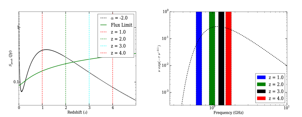
Figure 5: Left: peak flux versus redshift for the AO327 survey for model F illustrating the effect of absorption and Doppler shift of the observed frequency as described in the text. The black dashed line is the flux of the FRB. The different vertical lines correspond to different redshifts. In this case, we assumed $\alpha=-2$, EM = 3$\times 10^{6}$ cm^-6 pc and $T_{e}=8000$ K. Right: the different regions of the absorption spectrum probed by the survey at different redshifts. The different shaded regions correspond to the rest frame frequency probed by the survey at different redshifts.

5 Discussion

Our results suggest that telescopes in the 0.4–1.0 GHz band will make vital contributions to our understanding of FRBs. Even with free-free absorption and scattering playing a vital role in flux mitigation of FRBs, CHIME will be able to detect these bursts on a daily basis by the virtue of its extensive bandwidth and vast instantaneous sky coverage. We also looked into the possible caveats in the analysis and the effects those would have on the predictions for CHIME. Our investigation suggests that with all the caveats considered, the lowest yield for a future CHIME survey is $\sim 30$ FRBs per day which is very optimistic compared to expected yield from other surveys. For example, the corresponding yield for future UTMOST observations is about 1–2 FRBs per month for future observations which makes it difficult to differentiate between the two models at the moment.

We also discussed certain caveats in our analysis (§4.3) and how these assumptions affect the results. We found that a distribution in luminosities for FRBs, rather than a standard candle model assumed here, results in weaker constraints for the spectral indices of the population. Future surveys, however, will be excellent at probing the FRB luminosities through the dependence of luminosity on survey yield.

If the FRBs currently observed lie predominantly in the local Universe (i.e. have characteristic distances of 100 Mpc), then the large DMs cannot be accounted for by the Milky Way, host and IGM contributions. This discrepancy suggests that a large contribution to the DM comes from the local plasma around the source which favours models C and F as the most plausible scenarios describing these events. Assuming the parameters in model C, we can estimate the linear size of the absorber around the source in order to produce the high DMs observed for FRBs. If we take the FRB with the highest known DM (FRB 121002) and place it at $z=0.025$ then, assuming model C, we obtain a linear size of $\sim$ 1.4 pc. This is very similar to the parsec size high density filaments found in supernova remnants and magnetar ejecta (Lewandowski et al., 2015; Koo et al., 2007; Kulkarni et al., 2015). Thus, if future observations establish this distance scale for the FRB population, it should be possible to better constrain the model of absorption and the progenitor.

During the course of this work, we observed an interesting trend in the FRB flux as a function of redshift for observations in the $<1$ GHz band where models C and F predict an increase in flux density as a function of redshift (see, e.g., the left panel of Fig. 5). This behaviour is due to the Doppler shifting of a spectrum with a turn-over in its rest frame, which is a natural feature of the free-free absorption models. For sources at higher redshifts, we sample a different region in the spectrum of the source (see the right panel of Fig. 5). If the spectrum has a turnover, the peak flux increases as we sample the rising edge of the spectrum. At higher redshifts, the frequency band passes over the turnover resulting in a decrease in the peak flux as expected. As discussed in §4.3, we have not included the potential increase in the FRB rate with redshift that is predicted in cosmological models invoking star formation (Madau & Dickinson, 2014). If these models prove to be relevant in future, the aforementioned effect will be even stronger than seen in Fig. 5.

The constraints given in Table 2 can tell us about the nature of the FRB progenitors. The observed and predicted spectral indices suggest that FRB spectral indices are different from pulsar spectral indices which have a mean of -1.4 (Bates et al., 2014). Observations have suggested that at least some FRB spectral indices are positive (Spitler et al., 2016). Assuming a synchrotron source, the spectral index and the flux together can give us order of magnitude estimates about the magnetic field and effective electron temperature of the source (see for e.g Condon & Ransom, 2016). For example, if FRBs truly have a positive spectral index at frequencies of 1 GHz, the results favour a compact source with large magnetic field that is perpendicular to the line of sight (e.g., as seen in magnetar bursts) since the frequency at which the source becomes optically thick is proportional to the magnitude of the magnetic field while a negative spectral index would suggest other synchrotron sources (e.g., giant pulses from neutron stars). A large sample size of these sources expected from CHIME and HIRAX will definitely help to alleviate the problem.

In summary, we have carried out a detailed analysis of possible FRB source populations and the expected yield from ongoing and future radio surveys below 1 GHz, based on results from the previous surveys. The previous results help in constraining the spectral index of the burst although no inference on the emission model can be drawn currently. Even with the most stringent model, in which spectral turnovers are expected in the observing band, CHIME is expected to see FRBs very frequently. Similar results are expected to be seen by HIRAX. The yields of CHIME, HIRAX and UTMOST will undoubtedly lead to a large sample that will provide great insights into the nature of and emission mechanism of these enigmatic sources.

References

- Bates et al. (2014) Bates S. D., Lorimer D. R., Rane A., Swiggum J., 2014, MNRAS, 439, 2893
- Bhat et al. (2004) Bhat N. D. R., Cordes J. M., Camilo F., Nice D. J., Lorimer D. R., 2004, ApJ, 605, 759
- Caleb et al. (2016) Caleb M., Flynn C., Bailes M., Barr E. D., Bateman T., Bhandari S., Campbell-Wilson D., Green A. J., et al. 2016, MNRAS, 458, 718
- Caleb et al. (2016) Caleb M., Flynn C., Bailes M., Barr E. D., Hunstead R. W., Keane E. F., Ravi V., van Straten W., 2016, MNRAS, 458, 708
- Champion et al. (2016) Champion D. J., Petroff E., Kramer M., Keith M. J., Bailes M., Barr E. D., Bates S. D., Bhat N. D. R., et al. 2016, MNRAS
- Condon & Ransom (2016) Condon J., Ransom S., 2016, Essential Radio Astronomy. Princeton University Press
- Connor et al. (2016) Connor L., Lin H.-H., Masui K., Oppermann N., Pen U.-L., Peterson J. B., Roman A., Sievers J., 2016, MNRAS, 460, 1054
- Cordes et al. (2004) Cordes J. M., Bhat N. D. R., Hankins T. H., McLaughlin M. A., Kern J., 2004, ApJ, 612, 375
- Cordes & Wasserman (2016) Cordes J. M., Wasserman I., 2016, MNRAS, 457, 232
- Cordes et al. (2016) Cordes J. M., Wharton R. S., Spitler L. G., Chatterjee S., Wasserman I., 2016, ArXiv e-prints 1605.05890
- Crawford et al. (2016) Crawford F., Rane A., Tran L., Rolph K., Lorimer D. R., Ridley J. P., 2016, MNRAS
- Deneva et al. (2016) Deneva J. S., Stovall K., McLaughlin M. A., Bagchi M., Bates S. D., Freire P. C. C., Martinez J. G., Jenet F., Garver-Daniels N., 2016, ApJ, 821, 10
- Inoue (2004) Inoue S., 2004, MNRAS, 348, 999
- Karastergiou et al. (2015) Karastergiou A., Chennamangalam J., Armour W., Williams C., Mort B., Dulwich F., Salvini S., Magro A., et al. 2015, MNRAS, 452, 1254
- Katz (2016) Katz J. I., 2016, ArXiv e-prints 1604.01799
- Keane et al. (2016) Keane E. F., Johnston S., Bhandari S., Barr E., Bhat N. D. R., Burgay M., Caleb M., Flynn C., et el. 2016, Nature
- Koo et al. (2007) Koo B.-C., Moon D.-S., Lee H.-G., Lee J.-J., Matthews K., 2007, ApJ, 657, 308
- Kulkarni et al. (2015) Kulkarni S. R., Ofek E. O., Neill J. D., 2015, ArXiv e-prints 1511.09137
- Lewandowski et al. (2015) Lewandowski W., Rożko K., Kijak J., Melikidze G. I., 2015, ApJ, 808, 18
- Lorimer et al. (2007) Lorimer D. R., Bailes M., McLaughlin M. A., Narkevic D. J., Crawford F., 2007, Science, 318, 777
- Lorimer et al. (2013) Lorimer D. R., Karastergiou A., McLaughlin M. A., Johnston S., 2013, MNRAS, 436, L5
- Lorimer & Kramer (2004) Lorimer D. R., Kramer M., 2004, Handbook of Pulsar Astronomy. Cambridge University Press
- Lyutikov et al. (2016) Lyutikov M., Burzawa L., Popov S. B., 2016, ArXiv e-prints 1603.02891
- Macquart & Koay (2013) Macquart J.-P., Koay J. Y., 2013, ApJ, 776, 125
- Madau & Dickinson (2014) Madau P., Dickinson M., 2014, ARA&A, 52, 415
- Masui et al. (2015) Masui K., Lin H.-H., Sievers J., Anderson C. J., Chang T.-C., Chen X., Ganguly A., et al. 2015, Nature, 528, 523
- Newburgh et al. (2014) Newburgh L. B., Addison G. E., Amiri M., Bandura K., Bond J. R., Connor L., Cliche J.-F., Davis G., Deng M., et al. 2014, in Ground-based and Airborne Telescopes V Vol. 9145 of SPIE, Calibrating CHIME: a new radio interferometer to probe dark energy. p. 91454V
- Newburgh et al. (2016) Newburgh L. B., Bandura K., Bucher M. A., Chang T.-C., Chiang H. C., Cliche J. F., Dave R., Dobbs M., et al. 2016, ArXiv e-prints 1607.02059
- Petroff et al. (2015) Petroff E., Bailes M., Barr E. D., Barsdell B. R., Bhat N. D. R., Bian F., Burke-Spolaor S., Caleb M., et al. 2015, MNRAS, 447, 246
- Piro (2016) Piro A. L., 2016, ArXiv e-prints 1604.04909
- Rajwade et al. (2016) Rajwade K., Lorimer D. R., Anderson L. D., 2016, MNRAS, 455, 493
- Rowlinson et al. (2016) Rowlinson A., Bell M. E., Murphy T., Trott C. M., Hurley-Walker N., Johnston S., Tingay S. J., Kaplan D. L., et al. 2016, MNRAS, 458, 3506
- Spitler et al. (2014) Spitler L. G., Cordes J. M., Hessels J. W. T., Lorimer D. R., McLaughlin M. A., Chatterjee S., Crawford F., Deneva J. S., et al. 2014, ApJ, 790, 101
- Spitler et al. (2016) Spitler L. G., Scholz P., Hessels J. W. T., Bogdanov S., Brazier A., Camilo F., Chatterjee S., Cordes J. M., et al. 2016, Nature, 531, 202
- Stovall et al. (2014) Stovall K., Lynch R. S., Ransom S. M., Archibald A. M., Banaszak S., Biwer C. M., Boyles J., Dartez L. P., et al. 2014, ApJ, 791, 67
- Thornton et al. (2013) Thornton D., Stappers B., Bailes M., Barsdell B., Bates S., Bhat N. D. R., Burgay M., Burke-Spolaor S., et al. 2013, Science, 341, 53
- Tingay et al. (2015) Tingay S. J., Trott C. M., Wayth R. B., Bernardi G., Bowman J. D., Briggs F., Cappallo R. J., Deshpande A. A., et al. 2015, AJ, 150, 199
- Vedantham et al. (2016) Vedantham H. K., Ravi V., Hallinan G., Shannon R., 2016, ArXiv e-prints:1606.06795
- Yamasaki et al. (2016) Yamasaki S., Totani T., Kawanaka N., 2016, MNRAS, 460, 2875
- Zackay & Ofek (2014) Zackay B., Ofek E. O., 2014, ArXiv e-prints 1411.5373