All-phononic Amplification in Coupled Cantilever Arrays based on Gap Soliton Dynamics

Abstract

We present a mechanism of amplification of phonons by phonons on the basis of nonlinear band-gap transmission phenomenon. As a concept the idea may be applied to the various number of systems, however we introduce the specific idea of creating amplification scenario in the chain of coupled cantilever arrays. One chain is driven at the constant frequency located in the upper band of the ladder system, thus no wave enters the system. However the frequency is specifically chosen to be very close to the maximum value of frequency corresponding to dispersion relation of the system. Amplification scenario happens when a counter phase pulse of same frequency with a small amplitude is introduced to the second chain. If both signals exceed a threshold amplitude for the band-gap transmission a large amplitude soliton enters the system - therefore we have an amplifier. Although the concept may be applied in a variety of contexts - all optical or all-magnonic systems, we choose the system of coupled cantilever arrays and represent a clear example of the application of presented conceptual idea. Logical operations is the other probable field, where such mechanism could be used, which might significantly broaden the horizon of considered applications of band-gap soliton dynamics.

IIntroduction

The first documented observations of soliton waves occurred in 1834 by John Scott Russell, although the significance of soliton waves became clear later, with the studies of Korteweg - de Vries equation, ultimately brought mathematical clarity to the processes observed before.

As the studies on nonlinear phenomena went on, the numerical experiments on discrete nonlinear structures emerged. The first of those is known to be conducted by Fermi, Pasta and Ulam in 1954 fpu . The studies on FPU model and its developments klein ; braun ; toda led to the discovery of solitons flach0 ; zabusky ; thierry1 . The model of anharmonic oscillator chains became a strong tool for modeling and explaining phenomenas in various branches of physics and contributed to the fundamentals nonlinear wave phenomena scott ; flach01 as well as statistical physics izrailev ; ruffo1 , has been applied to explain thermal conductivity in various physical systems kaburaki ; bambi , contributed to understanding the interrelation between integrability and chaos chaos ; chaos1 , was used as a model for representing complex condensed matter systems flach1 ; flach2 and electric transmission lines trans ; trans1 .

The studies of phononics and advancements in phonon laser technology led to researches on phonon diodes laser ; laser1 ; diode ; diode1 ; diode2 ; diode3 and all-phonon transistors all ; acoust ; merab .

In this article we are going to consider a system of coupled cantilever arrays and apply non-linear band gap transmissionleon ; ramaz1 ; ramaz2 in order to achieve the amplification of weak acoustic waves.

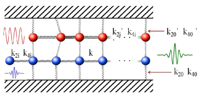
Figure 1: We have coupled FPU chains to represent the system of coupled cantilever arrays - the units of the chains represent the cantilevers, while the means of linking cantilevers one to another are represented by strings. Its also worth mentioning that we consider the system where any particular unit is not linked solely to its neighbors, but to any number of units in its neighborhood. The upper chain - red is driven with a constant frequency below the gap transmission value. A signal with a small amplitude is introduced to the bottom chain - blue, chosen so that the amplitude of both signals is enough to exceed the threshold value and a large amplitude soliton enters the system - green curve.

We study mono-element cantilever arrays, which consist of same cantilevers, which are connected to neighbors by means of the overhang, so that any particular cantilever can be observed as an oscillator [see Fig.2]. A number of works on wave propagation as well as logic operation tools have been made on the basis of cantilever arrays system canti ; canti1 ; canti2 . We are going to represent the system of coupled cantilever arrays by introducing a model of coupled FPU chains sievers1 , with on-site terms [Fig.1]; we also consider a system where any particular oscillator is linked to any number of oscillators in its neighborhood, although we are going to use six neighbors in numerical experiments. The idea behind the mechanism is driving one upper chain with a constant frequency just below the band gap transmission, while the bottom chain is at rest. We then introduce a pulse with a small amplitude to the lower chain with phase specifically chosen so that the overall amplitude of both signals is enough to exceed the threshold value. As a result large amplitude soliton enters into the system, thus we have amplification of a small acoustic signal.

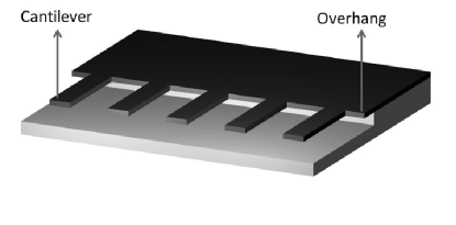
Figure 2: The scheme of a mono-element cantilever array. Exactly same cantilevers are linked by means of the overhang, thus any particular cantilever can be represented as an oscillator.

IIDeriving Analytical Solution for the Problem

IIIntroducing Equations of Motion

We begin with the Hamiltonian for system of coupled ladders with $N$ units each:

$$H=H_{u}+H_{w}+\frac{k}{2}(w_{n}-u_{n})^{2}$$ (1)

Where $H_{u}$:

$$H_{u}=\sum\limits_{n=1}^{N}\bigg{[}\frac{m{\dot{u}_{n}}^{2}}{2}+\sum\limits_{i=-N_{1}}^{N_{1}}\frac{k_{2i}}{2}(u_{n+i}-u_{n})^{2}+$$

$$\sum\limits_{i=-N_{1}}^{N_{1}}\frac{k_{4i}}{4}(u_{n+i}-u_{n})^{4}+\frac{k_{20}}{2}u_{n}^{2}+\frac{k_{40}}{4}u_{n}^{4}\bigg{]}$$ (2)

where $m$, $k$, $k_{2i}$, $k_{4i}$, $k_{20}$, $k_{40}$ are the parameters of the chain, namely, masses of units and stiffness coefficients of springs. Note that $H_{w}$ has the identical form with just other parameters except of $m$, which we consider the same for units in both ladders.We should point out that $N_{1}$ representing the number of units which are considered to interact with unit $u_{n}$ may vary. This fact brings up the possibility of describing the whole variety of systems using the pattern which is going to be considered below.

The equations of motion for $n$-th unit in each chain corresponding to the Hamiltonian $H$ will have the form of:

$$m\ddot{u}_{n} = \sum\limits_{i=-N_{1}}^{N_{1}}k_{2i}(u_{n+i}-u_{n})+\sum\limits_{i=-N_{1}}^{N_{1}}k_{4i}(u_{n+i}-u_{n})^{3}$$

$$+k_{20}u_{n}+k_{40}u_{n}^{3}+k(w_{n}-u_{n})$$

$$m\ddot{w}_{n} = k_{1}^{\prime}\sum\limits_{i=-N_{1}}^{N_{1}}k_{2i}^{\prime}(w_{n+i}-w_{n})+\sum\limits_{i=-N_{1}}^{N_{1}}k_{4i}^{\prime}(w_{n+i}-w_{n})^{3}$$ (3)

$$+k_{20}^{\prime}w_{n}+k_{40}^{\prime}w_{n}^{3}+k(u_{n}-w_{n})$$

IIDeriving the Solution

We use well-known approach, seeking the solution in a form of the following perturbative expansion:

$$\textbf{U}=\sum_{\alpha=1}^{\infty}\epsilon^{\alpha}\sum_{m=-\infty}^{+\infty}{\textbf{U}_{m}^{(\alpha)}(\tau,\xi)e^{im(pn-\Omega t)}}$$ (4)

where we define column vector $\textbf{U}^{(\alpha)}=(u_{n}^{(\alpha)},w_{n}^{(\alpha)})$, while $\xi$ and $\tau$ are slow variables introduced through: $\xi=\epsilon(n-vt)$ and $\tau=\epsilon t^{2}$; $v$ is a soliton group velocity defined below and $\epsilon$ is a small expansion parameter.

We go on with equating powers of $\epsilon$ substituting expansion (4) in set of equations (3). In the linear approximation we have the column vector $\textbf{U}_{1}^{(1)}\equiv\left(u_{n}^{(1)},w_{n}^{(1)}\right)=\varphi(\xi,\tau)\mathbf{R}$ and $\textbf{U}_{m}^{(1)}=0$ for $|m|\neq 1$; not restricting generality we can take a space-time independent column vector as $\mathbf{R}=\left(R,1\right)$, where $R$ is a complex number and $\varphi(\xi,\tau)$ is a scalar function of slow variables to be determined in the next approximations. Then by considering $\alpha=1$ (linear approximation) and the harmonic $m=1$ we arrive to the equation:

$$\hat{\mathbf{W}}*\mathbf{R}=0$$ (5)

where

$$\hat{\mathbf{W}}=\left(\begin{array}[]{cc}m\Omega^{2}+2s_{p}-k_{20}-k~{}~{}~{}~{}~{}~{}~{}~{}~{}~{}~{}~{}~{}~{}k{}{}{}{}{}{}{}{}{}{}{}{}{}\\ ~{}~{}~{}~{}~{}~{}~{}~{}~{}~{}~{}k~{}~{}~{}~{}~{}~{}~{}~{}~{}~{}~{}~{}~{}~{}m\Omega^{2}+2l_{p}-k_{20}^{\prime}-k\end{array}\right)$$ (8)

with

$$s_{p}=\sum\limits_{s=1}^{N_{1}}k_{2s}(\cos sp-1),l_{p}=\sum\limits_{l=1}^{N_{1}}k_{2l}^{\prime}(\cos lp-1)$$

The solvability of this equation demands Det($\hat{\mathbf{W}})=0$, which gives us two branches of dispersion relations:

$$\Omega^{2}_{1,2} = \frac{1}{m}\bigg{[}-s_{p}-l_{p}+\frac{1}{2}(k_{20}+k_{20}^{\prime})+k\pm$$ (9)

$$\pm \sqrt{(s_{p}-l_{p}+\frac{1}{2}(k_{20}-k_{20}^{\prime}))^{2}+k^{2}}\bigg{]}$$

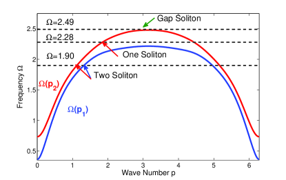
Figure 3: The dispersion relation for the considered system of two weakly coupled cantilever arrays. The blue and red curves represent dispersion relations for $p_{1}$ and $p_{2}$ respectively. As a result of these relations we consider three regimes: a)Two Soliton (lower dashed line), b)One soliton (middle dashed line), c) Amplification scenario (upper dashed line), with respective frequencies.

As a result of (9) we obtain two corresponding column vectors $\mathbf{R}_{j}=(R_{j},1)$ with $R_{j}$ expressed with the linear parameters of the problem $R_{j}=k/[k+k_{20}-m\Omega^{2}_{j}-2s_{p}]$, where $j=1,2$. Next we introduce a row vector $\mathbf{L}=(L,1)$ through the equation $\mathbf{L}*\hat{\mathbf{W}}=0$, that gives us two row vectors $\mathbf{L}_{j}$. In our case the respective components of row $\mathbf{L}_{j}$ and column $\mathbf{R}_{j}$ are identical $L_{j}=R_{j}$.Thus in linear limit we have following matrix relations:

$$\hat{\mathbf{W}}\left(\Omega_{j}\right)*\mathbf{R}_{j}=0,\qquad\mathbf{L}_{j}*\hat{\mathbf{W}}\left(\Omega_{j}\right)=0.$$ (10)

In the following for presentation clarity we omit the indexes $j$ and restore them at the end of the calculations. We go on with a second approximation ($\alpha=2$) substituting again (4) into (3) and considering first harmonic $m=1$, which leads us to the following equation:

$$\hat{\mathbf{W}}\textbf{U}^{(2)}+2i(\hat{\mathbf{B}}-m\Omega v\hat{\mathbf{I}})\frac{\partial\varphi}{\partial\xi}\mathbf{R}=0,$$ (11)

where

$$\hat{\mathbf{B}}=\left(\begin{array}[]{cc}\sum\limits_{s=1}^{N_{1}}sk_{2s}\sin sp&0\\ 0&\sum\limits_{l=1}^{N_{1}}lk_{2l}^{\prime}\sin lp\end{array}\right)$$ (14)

Then multiplying (11) by $\mathbf{L}$ one has

$$\mathbf{L}(\hat{\mathbf{B}}-m\Omega v\hat{\mathbf{I}})\frac{\partial\varphi}{\partial\xi}\mathbf{R}=0.$$ (15)

In order to identify constant $v$ in the equation above, let us take the derivative of (5) over $p$ and multiply then on the row vector $\mathbf{L}$. One gets:

$$\mathbf{L}\frac{\partial\hat{\mathbf{W}}}{\partial p}\mathbf{R}=2\mathbf{L}\left(m\frac{d\Omega}{dp}\Omega\hat{\mathbf{I}}-\hat{\mathbf{B}}\right)\mathbf{R}=0.$$ (16)

Comparing now (15) and (16) we immediately get the equality $v=\partial\Omega/\partial p$, thus the definition for group velocity, while from (11) one can solve $\textbf{U}^{(2)}$ as follows:

$$\textbf{U}^{(2)}=-2i\hat{\mathbf{W}}^{-1}(\hat{\mathbf{B}}-m\Omega v\hat{\mathbf{I}})\frac{\partial\varphi}{\partial\xi}\mathbf{R}.$$ (17)

In the third approximation, equating powers of $\epsilon$ for $\alpha=3$ and first harmonic $m=1$ we have:

$$\hat{\mathbf{W}}\textbf{U}^{(3)}+2i(\hat{\mathbf{B}}-m\Omega v\hat{\mathbf{I}})\frac{\partial\textbf{U}^{(2)}}{\partial\xi}+2im\Omega\frac{\partial\varphi}{\partial\tau}{\mathbf{R}}-$$ (18)

$$-\hat{\mathbf{C}}\frac{\partial^{2}\textbf{U}^{(1)}}{\partial\xi^{2}}+12\hat{\mathbf{P}}{\mathbf{N}}|\varphi|^{2}\varphi=0$$

where

$$\hat{\mathbf{C}}=mv^{2}\hat{\mathbf{I}}-\left(\begin{array}[]{cc}\sum\limits_{s=1}^{N_{1}}s^{2}k_{2s}\cos sp~{}~{}~{}~{}~{}0{}{}{}{}{}{}{}\\ ~{}~{}~{}0~{}~{}~{}~{}\sum\limits_{l=1}^{N_{1}}l^{2}k_{2l}^{\prime}\cos lp\end{array}\right)$$ (21)

$$\hat{\mathbf{P}}=\left(\begin{array}[]{cc}\sum\limits_{s=1}^{N_{1}}k_{4s}(1-\cos sp)^{2}+k_{40}~{}~{}~{}~{}~{}0{}{}{}{}{}{}{}\\ ~{}~{}~{}0~{}~{}~{}~{}\sum\limits_{l=1}^{N_{1}}k_{4l}^{\prime}(1-\cos lp)^{2}+k_{40}^{\prime}\end{array}\right)$$ (24)

$${\mathbf{N}}=\left(\begin{array}[]{cc}R^{3}\\ 1\end{array}\right)$$ (27)

Now noting that

$$2\left(\hat{\mathbf{B}}-m\Omega v\hat{\mathbf{I}}\right)\equiv-\frac{\partial\hat{\mathbf{W}}}{\partial p};$$

$$\quad\hat{\mathbf{C}}\equiv\frac{1}{2}\frac{\partial^{2}\hat{\mathbf{W}}}{\partial p^{2}}-m\Omega\frac{\partial^{2}\Omega}{\partial p^{2}}\hat{\mathbf{I}}$$ (28)

We can further simplify (II.2) multiplying it on $\mathbf{L}$ and taking into account (17) and (28):

$$\mathbf{L}\left(m\Omega\frac{\partial^{2}\Omega}{\partial p^{2}}\hat{\mathbf{I}}+\frac{\partial\hat{\mathbf{W}}}{\partial p}\hat{\mathbf{W}}^{-1}\frac{\partial\hat{\mathbf{W}}}{\partial p}-\frac{1}{2}\frac{\partial^{2}\hat{\mathbf{W}}}{\partial p^{2}}\right)\textbf{R}\frac{\partial^{2}\varphi}{\partial\xi^{2}}$$

$$+2im\Omega\frac{\partial\varphi}{\partial\tau}\mathbf{L}\mathbf{R}+12\mathbf{L}\hat{\mathbf{P}}{\mathbf{N}}|\varphi|^{2}\varphi=0$$ (29)

We can get a final form for (29) taking first and second derivatives of Eq. (5) over $p$:

$$\frac{\partial\hat{\mathbf{W}}}{\partial p}\mathbf{R}+\hat{\mathbf{W}}\frac{\partial\textbf{R}}{\partial p}=0;$$ (30)

$$\frac{\partial^{2}\hat{\mathbf{W}}}{\partial p^{2}}\mathbf{R}+2\frac{\partial\hat{\mathbf{W}}}{\partial p}\frac{\partial\textbf{R}}{\partial p}+\hat{\mathbf{W}}\frac{\partial^{2}\textbf{R}}{\partial p^{2}}=0$$

Solving now $\partial\textbf{R}/\partial p$ from the first equation and substituting it in the second one and then multiplying it on L one gets the following relation:

$$\mathbf{L}\frac{\partial\hat{\mathbf{W}}}{\partial p}\hat{\mathbf{W}}^{-1}\frac{\partial\hat{\mathbf{W}}}{\partial p}\textbf{R}-\frac{1}{2}\mathbf{L}\frac{\partial^{2}\hat{\mathbf{W}}}{\partial p^{2}}\mathbf{R}=0,$$ (31)

and now substituting this into the (29) and restoring indexes $j$-s one finally arrives to the Nonlinear Schrödinger (NLS) Equation for two nonlinear modes $j=1,2$:

$$2i\frac{\partial\varphi_{j}}{\partial\tau}+\Omega_{j}^{\prime\prime}\frac{\partial^{2}\varphi_{j}}{\partial\xi^{2}}-\Delta_{j}|\varphi_{j}|^{2}\varphi_{j}=0$$ (32)

where

$$\quad\Omega_{j}^{\prime\prime}={\frac{\partial^{2}\Omega_{j}}{\partial p^{2}}}\biggr{|}_{p=p_{j}},$$

$$\Delta_{j}=\frac{1}{m\Omega_{j}(1+R_{j}^{2})}\bigg{[}12R_{j}^{4}\sum\limits_{s=1}^{N_{1}}k_{4s}(1-\cos sp)^{2}+$$

$$+12\sum\limits_{l=1}^{N_{1}}k_{4l}^{\prime}(1-\cos lp)^{2}+R_{j}^{4}k_{40}+k_{40}^{\prime}\bigg{]}$$ (33)

and wavenumbers $p_{j}$ are the solutions of respective dispersion relations:

$$\Omega=\Omega_{j}+\Delta_{j}A_{j}^{2}/4$$ (34)

The solutions of (31) with respect to modes have solitonic form taniuti ; oikawa ; ramaz4

$$\left(u_{n}^{j},w_{n}^{j}\right)=\left(R_{j},~{}~{}1\right)\frac{A_{j}\cos(\Omega t-p_{j}n)}{\cosh\left[(n-v_{j}t)/\Lambda_{j}\right]}$$ (35)

where $A_{j}$ is a soliton amplitude, while soliton width $\Lambda_{j}$:

$$\Lambda_{j}=\frac{1}{A_{j}}\sqrt{\frac{2\Omega_{j}^{\prime\prime}}{\Delta_{j}}}$$ (36)

IIINumerical Experiments

IIIParameters

For the purpose of numerical experiments we are going to consider dimensionless parameters. We divide (3) by $k_{21}$ and introduce the following transformations:

$$x\longrightarrow x\sqrt{k_{21}/k_{41}},t\longrightarrow\sqrt{m/k_{21}}$$ (37)

After that we rescale the parameters of the chain and consider new dimensionless $k_{21}=1$ and $k_{41}=1$. Using (37) we obtain a new set of parameters (Table 1). Note the real parameters of the chain: $k_{21}=0.0828kg/s^{2}$, $k_{41}=4.0\times 10^{10}kg/s^{2}m^{2}$ $m=7.67\times 10^{-13}kg$. Thus by considering (37) and these parameters one can obtain the actual characteristics of the chain.

Table 1: We represent the parameters of considered coupled FPU chains: mass - m, $k_{20}$, $k_{40}$ - linear and qubic onsite terms respectively, $k_{21-26}$, $k_{41-46}$, linear and qubic intersite terms, as we consider six nearest neighbor oscillators of the every unit of the chain, $k$ - interchain term. Note that all of the parameters are obtained based on the characteristics of cantilever arrays sievers1

Parameter	Chain no.1	Chain no.2
$m$	1	1
$k_{20}$	0.1	0.17
$k_{21-26}$	1, 0.3720	1.3, 0.3297
	0.1304, 0.0489	0.1075, 0.0562
	0.0300, 0.0100	0.0272, 0.0106
$k_{40}$	0.2	0.7
$k_{41-46}$	1.0000, 0.3725	3.500, 1.3900
	0.1305, 0.0488	0.5771, 0.1505
	0.0300, 0.0100	0.0807, 0.0395
$k$	0.2	0.2

IIICombining Solutions

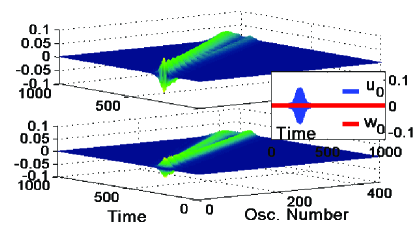
Figure 4: The two soliton regime: Combining solutions corresponding to two different modes(lower dashed line in [Fig.3]), we generate a soliton wave through the upper chain, while the lower chain is being at rest. As a result due to different velocities solitons depart from each other and propagate independently through the system. Corresponding frequency and amplitude: $\Omega=1.90,A=0.025$

Strictly speaking the linear combination of the solutions (35) of different $j=1$ and $j=2$ modes is not a solution of the initial nonlinear problem (3), however, in weakly nonlinear limit (small soliton amplitudes $A_{j}\ll 1$) and large relative group velocities $\left|v_{1}-v_{2}\right|/v_{1,2}\gtrsim 1$ one can combine the solutions (35) acquiring additional phase shift oikawa which could be safely neglected in the mentioned limits. By this one is able to construct the solution, which describes the initial excitation of the boundary of the solely upper chain. In particular, if one takes $A_{1}=A_{2}$ and finds such an excitation frequency that $v_{1}/\Lambda_{1}=v_{2}/\Lambda_{2}$, the combination $\left(u_{n}^{1},w_{n}^{1}\right)-\left(u_{n}^{2},w_{n}^{2}\right)$ at the origin $n=0$ gives

$$\left(u_{0}^{1},w_{0}^{1}\right)-\left(u_{0}^{2},w_{0}^{2}\right)=\left(R_{1}-R_{2},~{}~{}0\right)\frac{A_{1}\cos(\Omega t)}{\cosh\left[v_{1}t/\Lambda_{1}\right]},$$ (38)

thus driving both chains in time according to the above expression one can excite two soliton solution belonging to different branches. That is displayed in [Fig.4], driving in numerical simulations the left end of the upper chain $u_{0}$ with a frequency $\Omega=1.90$ and amplitude $A=\left(R_{1}-R_{2}\right)A_{1}$ with $A_{1}=0.025$ and calculating $R_{j}$ from Eq. (11). At the same time the lower chain is kept pinned at the left boundary ($w_{0}=0$) according again to the expression (38). As seen, the numerical test is just in tact with the expectation, as far as according to (35) we observe different amplitudes for the solitons in the upper chain and just the same $A_{1}=0.025$ in the lower one.

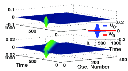
Figure 5: The one soliton regime: Combining soliton solution corresponding to $p_{1}$ with a soliton-like pulse with imaginary $p_{2}$ (39) (middle dashed line in [Fig.3]). As a result we generate one soliton wave through the upper chain. It then propagates freely into the system, while the first unit of the lower chain $w_{0}$ is at rest. Corresponding frequency and amplitude: $\Omega=2.28,A=0.025$

Next we examine one soliton generation driving again only upper chain with a frequency lying in the limits $\Omega_{2}(\pi)<\Omega<\Omega_{1}(\pi)$, particularly we apply $\Omega=2.28$ in numerical simulations (see middle horizontal line in [Fig.3]. In this case antisymmetric mode ($j=1$) solution could be again presented in solitonic form (35), while the symmetric mode ($j=2$) has no longer a solitonic profile, instead it is described by evanescent wave since the corresponding wavenumber $p_{2}$ is imaginary number (solution of dispersion relation $\Omega=\Omega_{2}(p)$ has no real roots):

$$\left(u_{n}^{2},w_{n}^{2}\right)=\left(R_{2},~{}~{}1\right)B(t)e^{-\left|p_{2}\right|n}\cos(\Omega_{2}t)$$ (39)

where $B(t)$ can slowly vary in time. This means that we observe only one soliton entering the chain. As we try to nullify oscillations in the lower chain $B(t)$ should take a form of $B(t)=A_{1}\rm sech\left(\emph{v}_{1}t/\Lambda_{1}\right)$ and then the combination $\left(u_{n}^{1},w_{n}^{1}\right)-\left(u_{n}^{2},w_{n}^{2}\right)$ at the origin $n=0$ gives the same form of the driving as in the previous case (38) of the two soliton generation. The results are displayed in [Fig.5], and as seen driving the upper chain with a frequency $\Omega=2.28$ now one monitors the generation of a single envelope soliton.

IIINumerical Experiments for Amplification Scenario

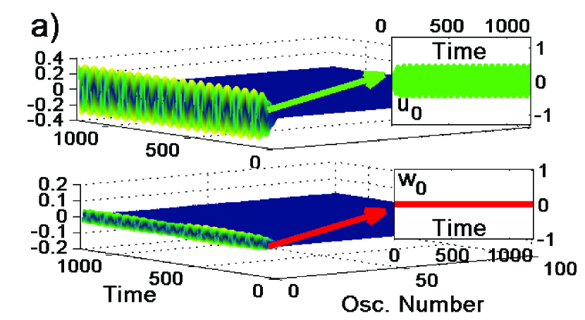
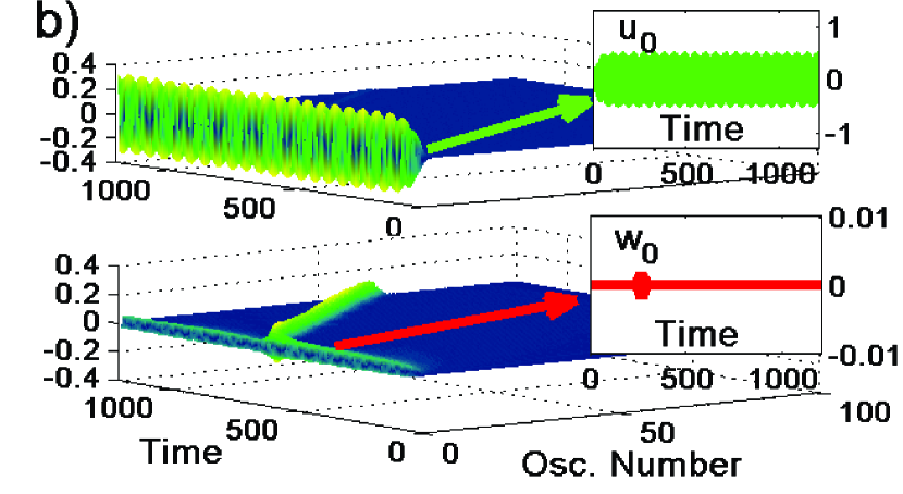
Figure 6: The amplification scenario: we consider driving frequency of the upper chain at $\Omega=2.49$ with $A=0.5098$, which is slightly above possible frequencies introduced through dispersion relation (upper dashed line in [Fig.3]). In both instances the insets show the motion of first unit of the chain - the source. a) - no wave enters the system as the first unit of the upper chain oscillates with given frequency and amplitude, while there is no excitation introduced to the lower chain. b) - a pulse with small amplitude - $A^{\prime}=0.004$ (41) is introduced through the lower chain. As a result the band gap soliton enters the system with amplitude of $A_{f}=0.3274$, thus giving the amplification of $80$ times at the output of the system.

Finally we consider the case $\Omega=2.49$ (upper dashed line in [Fig.3]) lying in the band gap of both modes, for which only evanescent wave solutions (39) is realized for the modes if the driving amplitude is small. However, if the amplitude exceeds some threshold value, a gap soliton can be created and propagate along the ladder. For the estimation of this threshold value, we assume that the upper chain is driven with the amplitude $A$ while the lower one is kept pinned.Then, looking at the typical solution of such a scenario (38) one can notice that the weight of the antisymmetric mode $A_{1}$ is defined from the relation $A=A_{1}\left(1-R_{1}/R_{2}\right)$ and the threshold value is calculated from the expression of nonlinear frequency shift (34). Thus a threshold amplitude for which driving of the upper chain produces a gap soliton could be straightforwardly derived as follows:

$$A_{th}=\left(1-R_{1}/R_{2}\right)\sqrt{4\left[\Omega-\Omega_{1}(\pi)\right]/\Delta_{1}}.$$ (40)

Determining $A_{th}$ gives us an opportunity to realize the amplification scenario. For this we create the continuous driving in the upper chain with a band-gap frequency $\Omega=2.49$ and amplitude just below the threshold, then even small counter-phase pulse in the lower chain can help to overcome the threshold and provide the necessary amplification effect for the weak pulse. Thus we choose the driving amplitude and estimate a pulse needed for a single gap soliton to enter the system using (34):

$$A^{\prime}=R_{1}\sqrt{4\left[\Omega-\Omega_{1}(\pi)\right]/\Delta_{1}}.$$ (41)

For the numerical experiment displayed in the [Fig.6] we use a continuous driving with the amplitude $A=0.5098$, while the pulse amplitude in the lower chain can be of the order of $0.004$. As seen such a small pulse is enough to create a gap soliton and realize amplification scenario in the oscillator ladder. Returning to dimension units we have $\nu=130.2MHz$ for frequency, $A=0.73\mu m$ $A^{\prime}=0.005\mu m$ for driving and pulse amplitude.

Concluding, a clear advantage of the proposed mechanism is that in a wide range of a weak signal shape and amplitude the generated output soliton amplitude keeps unchanged providing thus digital amplification scenario. Moreover, taking into account that we are using a single operational frequency, the output signal could be readily used for the further processing. Besides that, different geometries of the coupled chains could be proposed for implementing the developed mechanism of amplification for logic gate operations. We considered any number of interacting neighbor units and then applied theory for coupled cantilever arrays. Therefore one has possibilities of studying systems with any precision in terms of number of interacting neighbor units.

We thank A. Gurchumelia for creating clear visual scheme of a cantilever array [Fig.2].

References

- (1) E. Fermi, J. Pasta, S. Ulam, and M. Tsingou, in The Many-Body Problems, edited by D. C. Mattis (World Scientific, Singapore, 1993); The Fermi-Pasta-Ulam Problem: A Status Report, edited by G. Gallavotti (Springer, New York, 2008).
- (2) F. Abdullaev, V.V. Konotop, (eds.) Nonlinear Waves: Classical and Quantum Aspects, NATO Science Series II: Mathematics, Physics and Chemistry 153 (2005).
- (3) O.M. Braun, Y.S. Kivshar, The Frenkel-Kontorova Model: Concepts, Methods, and Applications, Springer (2004).
- (4) M. Toda, Jour. Phys. Soc. Japan 22, 431 (1967). M. Toda, Theory of Nonlinear Lattices, Springer (1978).
- (5) S. Flach, A. Gorbach, Chaos 15, 015112 (2005).
- (6) N.J. Zabusky, M.D. Kruskal, Phys. Rev. Lett. 15, 240-243 (1965).
- (7) T. Dauxois, M. Peyrard, Physics of Solitons, Cambridge University Press (2005).
- (8) A. Gorbach, S. Flach, Phys. Rev. E 72, 056607 (2005).
- (9) A.C. Scott (ed), Encyclopedia of Nonlinear Science, Routledge, New Yourk and London (2005).
- (10) F.M. Izrailev, B.V. Chirikov, Soviet Phys. Dokl. 11, 30 (1966).
- (11) R. Livi, M. Pettini, S. Ruffo, M. Sparpaglione, A. Vulpiani, Phys. Rev. A 28, 3544 (1985).
- (12) H. Kaburaki, M. Machida, Phys. Lett. A 181, 1 (1993).
- (13) Bambi Hu, Baowen Li, Hong Zhao, Phys. Rev. E 57, 2992 (1998).
- (14) Chaos, Focus Issue, 15, The ”Fermi-Pasta-Ulam” problem: the first fifty years, (2005).
- (15) Marco Pettini, Lapo Casetti, Monica Cerruti-Sola, Roberto Franzosi, E. G. D. Cohen, Chaos 15, 015106 (2005).
- (16) D.K. Campbell, S. Flach, Y.S. Kivshar, Physics Today, 43 (January 2004).
- (17) S. Flach, C.R. Willis, Phys. Rep. 295, 181 (1995).
- (18) D.S. Ricketts, D. Ham, Electrical Solitons: Theory, Design, and Applications, CRC Press (2011).
- (19) M. Sato, T. Mukaide, T. Nakaguchi, and A. J. SieversPhys. Rev. E 94, 012223
- (20) K. Vahala, M. Herrmann, S. Knünz, V. Batteiger, G. Saathoff, T. W. H nsch, Th. Udem, Nature Physics 5, 682 (2009).
- (21) A. Fainstein, N. D. Lanzillotti-Kimura, B. Jusserand, B. Perrin, Phys. Rev. Lett. 110 , 037403 (2013).
- (22) Liang et al., Nature, 9, 989 (2010).
- (23) Li et al., Phys. Rev. Lett. 106, 084301 (2011).
- (24) B. Liang, B. Yuan, J.-c. Cheng, Phys. Rev. Lett. 103, 104301 (2009).
- (25) N. Boechler, G. Theocharis, C. Daraio, Nature Materials, 10, 665 (2011).
- (26) B. Liang, W.-w. Kan, X.-y. Zou, L.-l. Yin, and J.-c. Cheng, Appl. Phys. Lett. 105, 083510 (2014).
- (27) D. Hatanaka, I. Mahboob, K. Onomitsu, and H. Yamaguchi, Appl. Phys. Lett., 102, 213102 (2013).
- (28) Merab Malishava, Ramaz Khomeriki Phys. Rev. Lett. 115, 104301.
- (29) M. Sato, Y. Sada, W. Shi, S. Shige, T. Ishikawa, Y. Soga, B. E. Hubbard, B. Ilic and A. J. Sievers, Chaos 25, 013103 (2015).
- (30) M. Sato and A. J. Sievers, Phys. Rev. Lett. 98, 214101 (2007).
- (31) M. Sato, B. E. Hubbard, A. J. Sievers, B. Ilic and H. G. Craighead, EPL, 66, 3 (2004).
- (32) F. Geniet, J. Leon, Phys. Rev. Lett. 89, 134102 (2002).
- (33) R. Khomeriki, Phys. Rev. Lett. 92, 063905 (2004).
- (34) R. Khomeriki, S. Lepri, S. Ruffo, Phys. Rev. E, 70, 066626 (2004).
- (35) M. Sato, B. E. Hubbard, and A. J. Sievers, Rev. Mod. Phys., 78, 137 (2006).
- (36) T. Taniuti, N. Yajima, J. Math. Phys. 10, 1369 (1969).
- (37) M. Oikawa and N. Yajima, J. Phys. Soc. Jpn. 37, 486 (1974).
- (38) N. Giorgadze, R. Khomeriki, Phys. Stat. Solidi (b), 207, 249 (1998).