Anisotropic residual based a posteriori mesh adaptation in 2D: element based approach

Abstract

An element-based adaptation method is developed for an anisotropic a posteriori error estimator. The adaptation does not make use of a metric, but instead equidistributes the error over elements using local mesh modifications. Numerical results are reported, comparing with three popular anisotropic adaptation methods currently in use. It was found that the new method gives favourable results for controlling the energy norm of the error in terms of degrees of freedom at the cost of increased CPU usage. Additionally, we considered a new $L^{2}$ variant of the estimator. The estimator is shown to be conditionally equivalent to the exact $L^{2}$ error. We provide examples of adapted meshes with the $L^{2}$ estimator, and show that it gives greater control of the $L^{2}$ error compared with the original estimator.

1 Introduction

In the last twenty years, anisotropic mesh adaptation has seen great activity. Since the work of D’Azevedo and Simpson in [13] and [12] for piecewise linear approximation of quadratic functions there has been a significant amount of research dedicated to producing practical adaptation procedures based on their results. In addition, there has been much software written for the implementation, which either construct an entirely new mesh, such as BAMG [22], BL2D [24], GAMANIC3D [18], or apply local modifications to a previous mesh, such as MEF++ [19], MMG3D [14], YAMS [31]. The main idea they share in common is to construct a non-Euclidean metric from the Hessian of the solution. We will refer to them as Hessian adaptation methods, see for instance [25], [26], [17], [7], [21].

Residual a posteriori error estimation for elliptic equations has been around for some time. In [2] and [3], Babuska and Rheinboldt introduced a local estimator, constructed entirely from the approximate solution, that is globally equivalent to the energy norm of the error. Numerical results showed that it was suitable for the purposes of mesh adaptation by determining regions in which the mesh could be refined or coarsened. While initially an entirely isotropic method, recently, the residual method was modernized by the introduction of anisotropic interpolation estimates from [15]. Unlike classical results, the new estimates did not require a minimum (or maximum) angle condition, and instead took into account the geometric properties of the element. In [32] and [16] these interpolation results were combined with the standard a posteriori estimates to drive mesh adaptation by constructing a metric. We will refer to this method as the residual metric method. The method results in highly anisotropic meshes, reducing the error by an order of magnitude compared to isotropic methods [32]. Moreover, the procedure has been successfully applied to a variety of nonlinear situations, including a reaction-diffusion system to model solutal dendrites in [9] and the Euler equations to model the supersonic flow over an aircraft in [8].

Recent work in [5] demonstrates the potential advantages of element-based anisotropic mesh adaptation over the usual metric based mesh adaptation methods used so far. The error estimator they use is hierarchical: from a given approximate solution, they construct a higher-order, more accurate approximation. For the Hessian method it is necessary to take the absolute value of the eigenvalues of the Hessian, thus treating positive and negative curvature as essentially equal, while the distinction can be seen very clearly in meshes adapted with the hierarchical method. Further, the hierarchical estimator has the advantage that it can naturally be applied to finite elements of arbitrary order.

The primary goal of this paper is to introduce, and numerically assess, an element-based adaptation approach to be used with the residual estimator from [32]. We will refer to this method as the element-based residual method. Motivation for implementing such a method includes avoiding the additional steps involved in converting the estimator defined on elements, to a metric defined on the nodes, during which information could be lost. Additionally, we would like to attempt to mimic the success of the hierarchical method. The adaptation will be implemented by interfacing the estimator with the hierarchical adaptation code MEF++. We also introduce a variant of the estimator for the $L^{2}$ norm error, which is shown to be reliable and efficient under certain assumptions, and show that the estimator is also suitable for anisotropic mesh adaptation. A secondary goal of the paper will be to provide a comparative performance analysis between four different adaptation techniques: element-based residual, metric based residual, Hessian, and hierarchical.

The outline of this paper is as follows: in Section 2 we introduce the model problem and error estimator, as well as recall some results from the literature; in Section 3 we discuss both the metric and element-based adaptation procedures; in Section 4 we produce numerical results, validating the element-based method, and comparing it with other anisotropic adaptation procedures.

2 The estimator

We discuss the model problem and introduce a residual estimator. Main results will be summarized from the literature. Full details can be found for instance in [15], [32], and [28].

2.1 Model problem

Let $\Omega\subseteq\mathbb{R}^{2}$ be a bounded polygonal domain, with boundary $\partial\Omega.$ Let $V=H^{1}(\Omega)$ and $V_{0}=\{v\in H^{1}(\Omega):v|_{\partial\Omega}=0\}$. For $g\in H^{1/2}(\partial\Omega)$, let $V_{g}=\{v\in H^{1}(\Omega):v|_{\partial\Omega}=g\}$, which may be thought of as the translation of $V_{0}$ by $g$. For $f\in L^{2}(\Omega),$ and a positive definite matrix $A$, let $u\in V_{g}$ be the solution of the equation

$$\left\{\begin{array}[]{ll}-\text{div}(A\nabla u)=f,&\quad\text{in }\Omega,\\ u=g,&\quad\text{on }\partial\Omega.\end{array}\right.$$ (1)

Then $u$ is the solution to the variational equation

$$B(u,v)=F(v),\quad\quad\forall v\in V_{0},$$

where

$$B(u,v) =\int_{\Omega}A\nabla u\cdot\nabla v\,\,\mathrm{d}x,\quad\quad u\in V_{g},v\in V_{0},$$

$$F(v) =\int_{\Omega}fv\,\,\mathrm{d}x,\quad\quad v\in V_{0}.$$

For $h>0$, let $\mathcal{T}_{h}$ be a conformal triangulation of $\Omega$ consisting of triangles $K$ with diameter $h_{K}\leq h.$ Denote by $V_{h}$ the finite element space of continuous, piecewise linear functions ($P_{1}$) on $\mathcal{T}_{h}$ and $V_{h,0}$ the subspace of functions vanishing on $\partial\Omega$. Let $g_{h}$ be a piecewise linear approximation of $g$ on $\partial\Omega$ and let $V_{h,g}=\{v_{h}\in V_{h}:v_{h}|_{\partial\Omega}=g_{h}\}.$ Then the finite element approximation $u_{h}\in V_{h,g}$ of $u$ satisfies the discrete variational equation

$$B(u_{h},v_{h})=F(v_{h}),\quad\quad\forall v_{h}\in V_{h,0}.$$ (2)

For details on the finite element method for elliptic problems, see for instance [34].

2.2 Anisotropic residual error estimator

Define the energy norm by ${\left|\kern-1.07639pt\left|\kern-1.07639pt\left|v\right|\kern-1.07639pt\right|\kern-1.07639pt\right|}=B(v,v)^{1/2}$ for $v\in V$. The residual mesh adaptation procedure is based on controlling the energy norm of the discretization error $e_{h}=u-u_{h}$. The error estimator, which will be outlined below, combines information of the residual with anisotropic interpolation estimates.

Define the localized residual by

$$R_{K}(u_{h})=f+\text{div}(A\nabla u_{h}),$$

where the divergence operator is local to $K$. The jump of the derivative for an element $K$ with edges $e_{i}$ is defined by

$$r_{K}(u_{h})=\sum_{i=1}^{3}[A\nabla u_{h}]_{e_{i}},$$

where the jump $[A\nabla v_{h}]_{e_{i}}$ over $e_{i}$ is defined as follows: denoting the outward unit normal by $n_{i}$ and the adjacent element (if it exists) by $K^{\prime}$, then

$$[A\nabla v_{h}]_{e_{i}}=\left\{\begin{array}[]{ll}0,&\quad e_{i}\in\partial\Omega,\\ A\nabla(v_{h})|_{K}\cdot n_{i}-A\nabla(v_{h})|_{K^{\prime}}\cdot n_{i},&\quad\text{otherwise}.\end{array}\right.$$

For a triangular element $K$, the anisotropic information comes from the affine mapping $F_{K}:\hat{K}\rightarrow K$. The reference element $\hat{K}$ is taken to be the equilateral triangle centred at the origin with vertices at the points $(0,1),\,(\frac{-\sqrt{3}}{2},\frac{-1}{2}),\,(\frac{\sqrt{3}}{2},\frac{-1}{2})$. The Jacobian $J_{K}$ of $F_{K}$ is non-degenerate, so the singular value decomposition (SVD) $J_{K}=\mathcal{R}_{K}^{T}\Lambda_{K}\mathcal{R}_{K}\mathcal{Z}_{K}$ consists of orthogonal matrices $\mathcal{R}_{K},\,\mathcal{Z}_{K}$, and positive definite diagonal matrix $\Lambda_{K}$. The matrices $\mathcal{R}_{K},\,\Lambda_{K}$ take the form

$$\mathcal{R}_{K}=\begin{pmatrix}r_{1,K}^{T}\\ r_{2,K}^{T}\end{pmatrix},\quad\quad\quad\Lambda_{K}=\begin{pmatrix}\lambda_{1,K}&&0\\ 0&&\lambda_{2,K}\end{pmatrix},$$

where $\lambda_{1,K}\geq\lambda_{2,K}>0$, $r_{1,K},\,r_{2,K}$ are orthogonal unit vectors. Geometrically, these eigenvalues and eigenvectors represent the deformation of the unit ball in $\mathbb{R}^{2}$ to an ellipse with axes of length $\lambda_{1,K},\,\lambda_{2,K}$ in directions $r_{1,K},\,r_{2,K}$ respectively. Moreover, they represent $K$ in the sense that the ellipse circumscribes the element.

Denote by $\Delta_{K}$ the patch of elements containing a vertex of $K.$ As noted in [29], for the bounds for the quasi-interpolation operator to be uniform, there must be an integer $\Gamma>0$ and a constant $C>0$ such that all such patch satisfies $\text{card}(\Delta_{K})\leq\Gamma$ (cardinality) and $\text{diam}(F_{K}^{-1}(\Delta_{K}))\leq C$ (diameter). For $v\in V,$ define the following “Hessian” type matrix:

$$\tilde{G}_{K}(v)=\left(\int_{\Delta_{K}}\frac{\partial v}{\partial x_{i}}\frac{\partial v}{\partial x_{j}}\,\,\mathrm{d}x\right)_{i,j},$$ (3)

and let

$$\tilde{\omega}_{K}(v)=(\lambda_{1,K}^{2}r_{1,K}^{T}\tilde{G}_{K}(v)r_{1,K}+\lambda_{2,K}^{2}r_{2,K}^{T}\tilde{G}_{K}(v)r_{2,K})^{1/2},$$

Finally, define

$$\hat{\eta}_{K}^{2} =\left(\|R_{K}(u_{h})\|_{0,K}+\left(\frac{h_{K}}{\lambda_{1,K}\lambda_{2,K}}\right)^{1/2}\|r_{K}(u_{h})\|_{0,\partial K}\right)\tilde{\omega}_{K}(e_{h}).$$ (4)

Theorem 1 ([32][33][28]).

There exist constants $C_{1,\hat{K}},\,C_{2,\hat{K}}>0$ such that

$$C_{1,\hat{K}}\sum_{K}\hat{\eta}_{K}^{2}\leq{\left|\kern-1.07639pt\left|\kern-1.07639pt\left|e_{h}\right|\kern-1.07639pt\right|\kern-1.07639pt\right|}^{2}\leq C_{2,\hat{K}}\sum_{K}\hat{\eta}_{K}^{2}.$$

The upper and lower bounds in Theorem 1 still depend on the unknown solution due to the $\tilde{\omega}_{K}(e_{h})$ term. The approach taken in [32] is to remove this dependency by using a gradient recovery operator of the form $\Pi:V_{h}\rightarrow V_{h}\oplus V_{h}.$ The operator should be super-convergent in the sense that $\Pi(u_{h})$ converges to $\nabla u$ faster than $\nabla u_{h}$, at least of order $1+\epsilon$ where $\epsilon>0$. For full details on the derivation of upper and lower bounds using super-convergence assumptions, see [28]. Therefore, for the remainder we replace $\tilde{G}_{K}(e_{h})$ by

$$G_{K}(u_{h})=\left(\int_{K}\left(\frac{\partial u_{h}}{\partial x_{i}}-\Pi(u_{h})_{i}\right)\left(\frac{\partial u_{h}}{\partial x_{j}}-\Pi(u_{h})_{j}\right)\,\mathrm{d}x\right)_{i,j},$$

and $\tilde{\omega}_{K}(e_{h})$ by $\omega_{K}(u_{h})=(\lambda_{1,K}^{2}r_{1,K}^{T}G_{K}(u_{h})r_{1,K}+\lambda_{2,K}^{2}r_{2,K}^{T}G_{K}(u_{h})r_{2,K})^{1/2}$ and the estimator becomes

$$\eta_{K}^{2} =\left(\|R_{K}(u_{h})\|_{0,K}+\left(\frac{h_{K}}{\lambda_{1,K}\lambda_{2,K}}\right)^{1/2}\|r_{K}(u_{h})\|_{0,\partial K}\right)\omega_{K}(u_{h}).$$ (5)

Note furthermore, that the integral for the matrix $\tilde{G}_{K}(e_{h})$ is taken on the patch $\Delta_{K}$ while that for $G_{K}(u_{h})$ is taken only on the element $K$. We found simplification works in practice and greatly reduces the computational complexity of the estimator, and has been used for instance in [32], [27].

2.3 Gradient recovery

Here we discuss briefly our choice of gradient recovery method. A popular choice is the simplified Zienkiewicz-Zhu (ZZ) operator, see [35], which generally performs very well. For instance, on certain regular meshes (parallel) it is asymptotically exact. Moreover, despite the fact that it cannot be proven to be super-convergent for non-regular meshes, in practice superconvergence has been observed for adapted meshes, as in [32] and [28].

An improved method is proposed by Zhang and Naga in [36]. The main idea is that for each node, one fits the solution values to a higher-order polynomial on a surrounding patch, the fit being obtained in a least-square sense. The value of the recovered gradient at the node is obtained by taking the gradient of the higher-order polynomial. They prove that the method is super-convergent for any regular mesh pattern, including situations where the ZZ estimator is not, such as the chevron pattern [35]. In addition, while the ZZ estimator only preserves polynomials of degree 1, their method can be extended to higher-order elements.

In this paper we have chosen to use the recovery method of Zhang and Naga due to an observed increase in performance. We remark that the usual justification of use of the ZZ estimator is its low cost. However, the gradient recovery is only computed once at the start of each iteration of the adaptation loop. As it turns out in our case, calculation of the Zhang/Naga gradient recovery accounted for less than $0.5$% of the total CPU time.

3 Adaptive procedure

In this section, we describe the four mesh adaptation methods that will be compared in Section 4, starting with the new, element-based adaptation procedure for the residual estimator $\eta_{K}.$ The section concludes with a discussion of the control of the $L^{2}$ norm error vs. the $H^{1}$ seminorm error.

3.1 Element-based adaptation

By Theorem 1, the estimator $\eta=\left(\sum_{K}\eta_{K}^{2}\right)^{1/2}$ is globally equivalent to the energy norm of the error ${\left|\kern-1.07639pt\left|\kern-1.07639pt\left|e_{h}\right|\kern-1.07639pt\right|\kern-1.07639pt\right|}$. Given an error tolerance $TOL>0,$ the adaptation algorithm will attempt to control the error so that $\eta\approx TOL$. Moreover, the mesh should have the least possible number of elements $N_{T}$. Therefore, the primary goal of the adaptation algorithm is to equidistribute the estimated error by asking that every element $K$ satisfies $\eta_{K}^{2}\approx\frac{TOL^{2}}{N_{T}}$. From an initial calculation of $\eta_{K}$ we adapt the mesh by performing the following local mesh modifications: edge refinement, edge swapping, node removal, and node displacement. For a complete description of local mesh modifications, see for instance [5], [11], [17], [21].

For convenience we define two element patches, which will be referred to frequently while discussing the local modifications. For an edge $e$, the patch $\Delta_{e}$ will denote the patch of elements containing $e$. Similarly, for a vertex $p$, the patch $\Delta_{p}$ will denote the patch of elements containing $p$.

3.1.1 Edge Refinement

Edge refinement is used to decrease the level of error where it is too large. The candidate edges for refinement are those belonging to an element $K$ for which $\eta_{K}^{2}>1.5\frac{TOL^{2}}{N_{T}}.$ For such an edge $e$ with associated edge patch $\Delta_{e}$, denote by $\Delta_{e}^{\prime}$ the resulting patch after refining $e$, and suppose they have respectively $N_{T,e},$ $N_{T,e^{\prime}}$ elements. Denote respectively by $\eta_{\Delta_{e}}^{2}$ and $\eta_{\Delta_{e}^{\prime}}^{2}$ the error on the patch before and after refinement. The refinement is accepted if the new error is closer to the goal in the following sense:

$$\left|\frac{\eta_{\Delta_{e}^{\prime}}^{2}}{N_{T,e^{\prime}}}-\frac{TOL^{2}}{N_{T}}\right|<\left|\frac{\eta_{\Delta_{e}}^{2}}{N_{T,e}}-\frac{TOL^{2}}{N_{T}}\right|.$$ (6)

3.1.2 Edge swapping

Edge swapping is used to minimize the error without changing the number of elements. For an internal edge $e$, consider the edge patch $\Delta_{e}$, test the reconnection of the edge, and denote this patch $\Delta_{e^{\prime}}$. Note that it may be geometrically impossible to swap an edge, for instance if the patch is not convex, or degenerates to a triangle. Edge swapping is performed if the global error decreases. At first, one might try swapping if the following criterion holds:

$$\sum_{K^{\prime}\in\Delta_{e^{\prime}}}\eta_{K^{\prime}}^{2}<\sum_{K\in\Delta_{e}}\eta_{K}^{2}.$$

However, for the residual estimator, the above criteria is not enough, and we had to enlarge the patch as in Figure 1. Note that swapping the edge changes the normal jump of the derivative for elements adjacent to $\Delta_{e}$. Including these elements in the error calculation means that we have included all elements for which $\eta_{K}$ is changed by swapping, so that if the error decreases on the patch, then in fact the error will have decreased globally.

Figure 1: Extension of the edge patch for edge swapping.

The edges are stored in an ordered list, and edge swapping is carried out by looping over this list and checking all internal edges. When an edge is swapped, the new edge is placed at the end of the list, so will be considered for swapping again. After the list is exhausted, if any edges were swapped the entire procedure will be repeated.

We remark that the loop will in fact terminate. There are only finitely many ways to reconfigure the mesh by swapping, and the edges are only swapped if the global error decreases. Furthermore, because no interpolation of the solution takes place during edge swapping, the map from edge configuration to global error calculation is well-defined, so it is not possible to arrive at a previous configuration but with smaller error. Also, as noted on p. 1339 of [32], the choice of reference element means that the contribution of the SVD will not depend on a reordering of the nodes.

3.1.3 Node removal

Node removal is used to reduce the number of mesh elements where possible, particularly where the error is small. Node removal consists in removing a node $p$ from the mesh, as well as the patch of elements, $\Delta_{p}$, attached to the node. The resulting “hole” then is remeshed, and we will call the resulting patch $\Delta_{p}^{\prime}$. The initial choice of remeshing is not important because the optimal choice will be determined by edge swapping. One compares the error before and after the procedure, denoted $\eta_{\Delta_{p}},$ $\eta_{\Delta_{p}^{\prime}}$, and the node is accepted for removal if the following analogue to (6) holds

$$\left|\frac{\eta_{\Delta_{p}^{\prime}}^{2}}{N_{T,p^{\prime}}}-\frac{TOL^{2}}{N_{T}}\right|<\left|\frac{\eta_{\Delta_{p}}^{2}}{N_{T,p}}-\frac{TOL^{2}}{N_{T}}\right|.$$ (7)

3.1.4 Node displacement

The goal of node displacement is to equidistribute the error over the mesh elements. Node displacement is applied to each vertex $p$ to determine the optimal position of the vertex within the vertex patch $\Delta_{p}$. Note that this patch might not be convex, so care has to be taken to avoid overlapping elements. We consider the value of the error on the elements as a discrete distribution, and find the position within the patch which minimizes the variance: $\min_{p}\left(\text{Var}_{K\in\Delta_{p}}\{\eta_{K}^{2}\}\right).$ No attempt is made to solve the minimization problem fully for each vertex, but only to find an approximate solution with one iteration of a gradient recovery method. Computing the full solution could be costly, and moreover might not even be possible depending on the shape of the function being minimized. Instead, one applies several iterations of the global node displacement procedure. As we will see in Section 3.2, node movement minimizes a different function in the hierarchical method from [5].

Edge refinement and node removal work towards achieving the error tolerance, node movement “smooths” the mesh by equidistributing the error, while edge swapping minimizes the error.

After a mesh operation is performed the error estimator needs to be recalculated. First we interpolate the continuous data, which in this case is $u_{h}$ and the recovered gradient $\Pi(u_{h}).$ The discontinuous data needs to be recalculated on each element, i.e. the singular value decomposition, discontinuous gradient, jump of the derivative, and the residual. Additionally, after each operation is performed there is a check to ensure degenerate elements were not produced.

All numerical results are produced with MEF++. The hierarchical estimator adaptation driver was used, described in [5], suitably adjusted.

3.2 Hierarchical

We summarize the ideas from [5]. Given a $P_{k}$ approximation $u_{h,k},$ construct a higher-order solution $P_{k+1}$, $\tilde{u}_{h,k+1}$, which is supposed to be more accurate. From this, one obtains an approximation of the error

$$e_{h}\approx\tilde{u}_{h,k+1}-u_{h,k}.$$ (8)

Taking $k=1$, and the barycentric representation of the element $K$ by $u_{h,1}|_{K}=u_{1}\lambda_{1}+u_{2}\lambda_{2}+u_{3}\lambda_{3}$, one builds $\tilde{u}_{h,2}$ in the “hierarchical” basis

$$\tilde{u}_{h,2}|_{K}=u_{1}\lambda_{1}+u_{2}\lambda_{2}+u_{3}\lambda_{3}+4(e_{1}\lambda_{1}\lambda_{2}+e_{2}\lambda_{1}\lambda_{3}+e_{3}\lambda_{2}\lambda_{3}),$$

where $e_{i}$ denotes the mid-edge values. Taking the Zhang-Naga (or any other sufficiently accurate) recovered gradient $\Pi(u_{h,1})=(\Pi(u_{h,1})_{1},\Pi(u_{h,1})_{2})$, the mid-edge values are found by enforcing consistency between the Hessian of $\tilde{u}_{h,2}$ and the derivatives of $\Pi(u_{h})$:

$$\frac{\partial^{2}\tilde{u}_{h,2}}{\partial x_{1}^{2}}=\frac{\partial\Pi(u_{h,1})_{1}}{\partial x_{1}},\quad\quad\frac{\partial^{2}\tilde{u}_{h,2}}{\partial x_{2}^{2}}=\frac{\partial\Pi(u_{h,1})_{2}}{\partial x_{2}},$$

$$\frac{\partial^{2}\tilde{u}_{h,2}}{\partial x_{1}\partial x_{2}}=\frac{1}{2}\left(\frac{\partial\Pi(u_{h,1})_{1}}{\partial x_{2}}+\frac{\partial\Pi(u_{h,1})_{2}}{\partial x_{1}}\right).$$

Having computed the higher-order solution, the adaptation process follows similarly to that used in Section 3.1. But since (8) gives a direct representation of the error field, one has considerably more freedom in how to calculate the error on each element. The choice in [5], and as implemented by the authors in MEF++, is to target the global error in the $L^{2}$ norm. The operations of edge refinement and node removal will be used to achieve a global level of error, while node displacement and edge swapping are used to locally equidistribute the error by minimizing the gradient of the error, i.e. the $H^{1}$-seminorm error.

In this paper, we only consider hierarchical adaptation for $P_{1}$ finite elements for the sake of comparison. However, note that (8) is quite general, and it is very easy to generalize these ideas to higher-order finite elements. The hierarchical method has been successfully applied to $P_{2}$ finite elements in [6].

3.3 Metric adaptation

Currently, the most popular anisotropic mesh adaptation methods in use are metric based. Here, the main idea is to control the edge length in a Riemannian metric. For a planar domain $\Omega$, an inner product is given by a set $\{\mathcal{M}(x)|x\in\Omega\}$ of $2\times 2$ positive definite matrices. In practice we only have a discrete approximation, consisting of a metric defined at the nodes of the mesh, the values at other points being obtained by interpolation [7]. For an edge $e=PQ$, the edge length is given by

$$|e|_{\mathcal{M}}=\int_{0}^{1}\sqrt{e^{T}\mathcal{M}(P+te)e}\,\,\mathrm{d}t.$$ (9)

The goal of a metric based adaptation algorithm will be to generate meshes which are “unit” with respect to the metric. For 2D meshes this simply means that, up to some tolerance, the edges have unit length.

The metric adaptation will be done using MEF++, applying the same mesh modification operations discussed Section 3.1. The goal of edge refinement and node removal is to achieve unit edge length, while the second two locally equidistribute the error. More precisely, edge swapping applies a non-Euclidean variant of the classical Delaunay edge swapping criterion to maximize the minimum angle. For node movement, the edges attached to a node are seen as a network of springs with stiffness proportional to metric edge length, and the goal is to minimize the “energy” of the system. For full details see for instance [21].

3.4 Residual metric based

Now we describe how the residual estimator introduced in Section 2 can be used to define a metric. There exist at least two approaches used in the literature, both following similar principles. The one we will use is that from [28] since it resulted in unit meshes in only a few iterations. The metric is constructed locally for the element $K$ by finding the shape of a new element $K_{new}$ which minimizes $\eta_{K_{new}}$ up to a fixed area. From [28], Proposition 26, the minimizing shape is given by $\tilde{r}_{1,K}=p_{2},\,\tilde{r}_{2,K}=p_{1},$ and $\tilde{s}_{K}=\sqrt{\frac{\alpha_{1,K}}{\alpha_{2,K}}},$ where $\alpha_{1,K}\geq\alpha_{2,K}>0$ and $p_{1},\,p_{2}$ are respectively the eigenvalues and eigenvectors of the normalized matrix $\frac{G_{K}}{|K|}.$ Under these conditions, one obtains a simple relation for the error [28, p. 826]. Imposing $\eta_{K}\equiv\tau$, where $\tau>$ is the local error tolerance, one determines the area from this relation, and then easily recovers the optimal values $\tilde{\lambda}_{1,K}$, $\tilde{\lambda}_{2,K}$. Finally, defining $\tilde{R}_{K},\,\tilde{\Lambda}_{K}$ in the obvious way, the metric on $K$ is then given by $\tilde{\mathcal{M}}_{K}=\tilde{R}_{K}^{T}\tilde{\Lambda}_{K}^{-2}\tilde{R}_{K}.$ We remark that the mesh adaptation software used for this paper requires the metric to be defined on vertices, and for this purpose we apply metric intersection. For a vertex $p$, the metric $\tilde{\mathcal{M}}_{p}$ will be defined as the intersection of all the metrics $\tilde{\mathcal{M}}_{K}$ over the patch $\Delta_{p}.$ For details on metric intersection, see for instance [17]. Note that, alternatively to metric intersection, we found that a simple averaging procedure gave satisfactory results.

3.5 Hessian

The Hessian metric approach introduced here follows the expositions from [7], [21]. The $P_{1}$ interpolation error $e_{h}^{I}=u-I_{h}(u)$ of a function $u$ on an edge $\ell=[x_{i},x_{j}]$ satisfies

$$|e_{h}^{I}|_{L^{\infty}(\ell)}=\frac{|\ell|^{2}}{8}\left|\frac{\mathrm{d}^{2}u}{\mathrm{d}x^{2}}(\xi)\right|,$$

where $\xi$ is some point in $\ell.$ The error on the edge can then approximated using the end-points of the interval

$$|e_{h}^{I}|_{L^{\infty}(\ell)}\approx\frac{1}{2}\left(\ell^{T}|H(x_{i})|\ell+\ell^{T}|H(x_{j})|\ell\right),$$ (10)

where $H(x)$ is the Hessian of $u$ at $x,$ and $|H(x)|$ is the positive semi-definite matrix obtained by taking the absolute value of the eigenvalues of the symmetric matrix $H(x)$. Fixing an error level $e_{D},$ defining the metric $\mathcal{M}_{x}=\frac{1}{8\cdot e_{D}}|H(x)|$, and computing the edge length from (9) with the trapezoid rule give $|\ell|_{\mathcal{M}}=1$ precisely when the approximate error (10) is equal to $e_{D}.$ For a slightly different approach to Hessian methods, see [25] and [26].

Note that (10) depends on the unknown Hessian of the solution. One may obtain a piecewise linear approximation of the Hessian from the computed solution, for instance, with the least square fitting method used in [4].

3.6 $L^{2}$ error vs. $H^{1}$ seminorm error estimation

While the residual estimator targets the energy norm of the error, it is also interesting to determine whether we can expect to control the $L^{2}$ norm of the error. Recall that for elliptic problems such as (1), if a set of meshes uniformly satisfies the minimum (or maximum) angle condition for some angle $\theta>0,$ then there exists $C_{1}>0$ such that for any such mesh with maximum edge length $h>0$,

$$|e_{h}|_{1,\Omega}\leq C_{1}h.$$ (11)

Furthermore, the Aubin-Nitsche Lemma states that there is a $C_{2}>0$ such that the $L^{2}$ error satisfies

$$\|e_{h}\|_{0,\Omega}\leq C_{2}h|e_{h}|_{1,\Omega}.$$ (12)

Combining (11) with (12) one concludes that there is a $C_{3}>0$ such that

$$\|e_{h}\|_{0,\Omega}\leq C_{3}h^{2}.$$ (13)

Therefore, if we adapt the mesh to control the $H^{1}$ seminorm error, which is the case for the residual estimator, we expect higher-order convergence for the $L^{2}$ error coming from an upper bound similar to (13).

In the absence of an Aubin-Nitsche Lemma in the context of anisotropic meshes, we attempt to find a comparison at the element level between the $L^{2}$ and energy norm of the error. The ultimate goal of the analysis is to derive an $L^{2}$ norm variant of the residual estimator $\eta_{K}$, which could be used for mesh adaptation.

To motivate our results, we first recall two existing a posteriori $L^{2}$ error estimators. The first, in the isotropic setting is of the form $\eta_{L^{2}(K)}=h_{K}\eta_{H^{1}(K)},$ where $\eta_{H^{1}(K)}$ is an estimator for the energy norm, see (3.20) and (3.31) from [1] and 5.1 from [10]). Similarly, the authors in [23] derived an anisotropic estimate of the form $\tilde{\eta}_{E}=(h_{\min,E})\eta_{E}$, where $\eta_{E},\,\tilde{\eta}_{E}$ are respectively estimates for the $H^{1}$ seminorm and $L^{2}$ norm of the error for the edge $E$, and where $h_{\min,E}$ plays an analogous role to $\lambda_{2,K}$ in the current setting. These observations lead us to propose the following candidate for an $L^{2}$ error estimator:

$$\tilde{\eta}_{K}=\lambda_{2,K}\eta_{K},$$ (14)

where $\eta_{K}$ is the energy norm estimator (5). In what follows we present some partial results towards the reliability and efficiency of this estimator.

We make the following strong assumption on the equivalence of the energy norm error: there exist $C_{1},\,C_{2}>0$ such that for every element $K$,

$$C_{1}\eta_{K}\leq|e_{h}|_{1,K}\leq C_{2}\eta_{K}.$$ (15)

Given this assumption, the strategy will be to relate the $L^{2}$ error and energy norm locally. Note that in the literature, the upper bound in (15) only appears globally (for the entire domain $\Omega$), while the lower bound holds on a patch related to a quasi-interpolation operator, see [28, Propositions 16, 21]. Numerical results in Section 4.1.1 suggest that provided the mesh is not too coarse, the inequality holds with $C_{1}=1$ and $C_{2}=10$, see Figure 4.

We begin with a technical lemma. In what follows we let $W_{h}$ denote the space of continuous piecewise quadratic functions on $\mathcal{T}_{h}$. We note, however, that $W_{h}$ could be replaced by a higher-order finite element space, with different constants for the inequalities.

Lemma 1.

Let $v_{h}\in V_{h}$.

1. There exists $C_{\hat{K}}>0$ depending only on the reference element $\hat{K}$ such that for all $w_{h}\in W_{h}$ and $K\in\mathcal{T}_{h}$,

   $$\|v_{h}-w_{h}\|_{0,K}\geq \,C_{\hat{K}}\lambda_{2,K}|v_{h}-w_{h}|_{1,K}.$$ (16)

2. Suppose that $w_{h}\in W_{h}$ and $C_{\hat{K},1}>0$ such that for all $K\in\mathcal{T}_{h}$

   $$\lambda_{1,K}\|\nabla(v_{h}-w_{h})\cdot r_{1,K}\|_{0,K} \leq C_{\hat{K},1}\lambda_{2,K}\|\nabla(v_{h}-w_{h})\cdot r_{2,K}\|_{0,K}.$$ (17)

   Then there exists $C_{\hat{K}}>0$ depending only on the reference element $\hat{K}$ and $C_{\hat{K},1}$ such that for all $K\in\mathcal{T}_{h}$,

   $$\|v_{h}-w_{h}\|_{0,K} \leq C_{\hat{K},2}\lambda_{2,K}|v_{h}-w_{h}|_{1,K}.$$ (18)

Proof.

By [15], Lemma 2.2 we have

$$|w_{h}-v_{h}|_{1,K} \leq\left(\frac{\lambda_{1,K}}{\lambda_{2,K}}\right)^{1/2}|\hat{w}_{h}-\hat{v}_{h}|_{1,\hat{K}},$$

where $\hat{w}=w\circ F_{K}$ for a function $w$ on $K.$ Since $P_{2}(\hat{K})$ is finite dimensional, there exist positive constants $\tilde{C}_{1},\,\tilde{C}_{2}$ such that

$$\tilde{C}_{1}\|\hat{w}\|_{0,\hat{K}}\leq|\hat{w}|_{1,\hat{K}}\leq\tilde{C}_{2}\|\hat{w}\|_{0,\hat{K}},\quad\quad\forall\hat{w}\in P_{2}(\hat{K}).$$

Therefore,

$$|w_{h}-v_{h}|_{1,K} \leq\tilde{C}_{2}\left(\frac{\lambda_{1,K}}{\lambda_{2,K}}\right)^{1/2}\|\hat{w}_{h}-\hat{v}_{h}\|_{0,\hat{K}}$$

$$=\tilde{C}_{2}\left(\frac{1}{\lambda_{1,K}\lambda_{2,K}}\right)^{1/2}\left(\frac{\lambda_{1,K}}{\lambda_{2,K}}\right)^{1/2}\|w_{h}-v_{h}\|_{0,K}$$

$$=\frac{\tilde{C}_{2}}{\lambda_{2,K}}\|w_{h}-v_{h}\|_{0,K},$$ (19)

and (16) follows. For (18), we have

$$\|v_{h}-w_{h}\|_{0,K} =\left(\lambda_{1,K}\lambda_{2,K}\right)^{1/2}\|\hat{u}_{h}-\hat{u}_{h,2}\|_{0,\hat{K}}$$

$$\leq\tilde{C}_{1}\left(\lambda_{1,K}\lambda_{2,K}\right)^{1/2}|\hat{u}_{h}-\hat{u}_{h,2}|_{1,\hat{K}}.$$

Applying [15], equation (17) to the right side of the inequality, and applying assumption (17),

$$\|v_{h}-w_{h}\|_{0,K}$$

$$\leq\tilde{C}_{1}\left(\lambda_{1,K}^{2}\|\nabla(v_{h}-w_{h})\cdot r_{1,K}\|_{0,K}^{2}+\lambda_{2,K}^{2}\|\nabla(v_{h}-w_{h})\cdot r_{2,K}\|_{0,K}^{2}\right)^{1/2}$$

$$\leq\tilde{C}_{1}C_{\hat{K},1}\lambda_{2,K}|v_{h}-w_{h}|_{1,K}.$$

∎

In the present situation we take $v_{h}=u_{h}.$ To apply Lemma 1 in a meaningful way, we would like to find functions $\{w_{h}\in W_{h}\}_{h}$ that converge to $u$ faster than $\{u_{h}\in V_{h}\}_{h}$ and that moreover satisfy (17) uniformly. Let $g_{h}=\Pi_{h}(u_{h})$ denote the recovered gradient, which is assumed to be superconvergent. In the literature, the adaptive algorithm is designed to achieve the equality

$$\lambda_{1,K}\|(\nabla u_{h}-g_{h})\cdot r_{1,K}\|_{0,K}=\lambda_{2,K}\|(\nabla u_{h}-g_{h})\cdot r_{2,K}\|_{0,K},$$

In the context of [28], this equality means that $\eta_{K}$ has been minimized with respect to the choice of $r_{1,K},\,r_{2,K}$ and aspect ratio $s_{K}$. The adaptive algorithm discussed in Section 4.1.1 will ensure that the equality holds by minimizing of $\eta_{K}$ with edge swapping and node movement. In general, $g_{h}$ is not the gradient of a function in $W_{h}$. Instead, we take $\tilde{u}_{h,2}\in W_{h}$ to be the hierarchical reconstruction introduced in [5], which in practice provides a higher-order approximation to $u$, for instance [5, Figure 17]. Additionally, it will be assumed that $\nabla\tilde{u}_{h,2}$ and $g_{h}$ are close enough so that (17) holds with $w_{h}=\tilde{u}_{h,2}.$

Proposition 1.

With the notation and assumptions of the preceding paragraph, there exist positive constants $C_{\hat{K},1},\,C_{\hat{K},2}$ such that for all $K\in\mathcal{T}_{h}$,

$$\|e_{h}\|_{0,K} \geq C_{\hat{K},1}\left(\lambda_{2,K}|e_{h}|_{1,K}-\|u-\tilde{u}_{h,2}\|_{0,K}-\lambda_{2,K}|u-\tilde{u}_{h,2}|_{1,K}\right),$$ (20)

and

$$\|e_{h}\|_{0,K} \leq C_{\hat{K},2}\left(\lambda_{2,K}|e_{h}|_{1,K}+\|u-\tilde{u}_{h,2}\|_{0,K}+\lambda_{2,K}|u-\tilde{u}_{h,2}|_{1,K}\right)$$ (21)

Proof.

This follows directly from Lemma 1 and straightforward triangle inequality arguments. ∎

Finally, if we apply the superconvergence assumptions on $\tilde{u}_{h,2}$ and $\nabla\tilde{u}_{h,2}$, and the strong energy norm error assumption (15), we conjecture that there exists $C_{\hat{K},1},\,C_{\hat{K},2}>0$ such that for every element $K,$ up to the addition of higher-order terms, the $L^{2}$ norm error satisfies

$$C_{\hat{K},1}\tilde{\eta}_{K}\leq\|e_{h}\|_{0,K}\leq C_{\hat{K},2}\tilde{\eta}_{K}.$$ (22)

This local estimate will be verified numerically in the following section.

4 Numerical results

In this section we provide numerical validation for the new, element-based adaptation method for the residual estimator. The full adaptation loop is given in Algorithm 1. The first test case will begin with an illustration of the convergence of the loop for the element-based residual method introduced in this paper, the notion of convergence to be made more precise in the following section. Next, we will assess how well the method performs in achieving the goal of equidistributing the error over the elements of the mesh. Since what we are really interested in is controlling the actual error, the analysis will include an element-level comparison of the estimated versus exact error. Following will be a numerical validation of the $L^{2}$ error control results from Section 3.6. Finally, the remainder of the section will be devoted to the comparison of the adaptation methods outlined in Section 3.

Algorithm 1 Solution-adaptation loop

1. Compute the solution and error estimator on the current mesh.

2. Adapt the current mesh by performing the following loop one or more times:

   1. Refine edges where the error is too large.

   2. Minimize the error by swapping edges until the algorithm terminates, then equidistribute the error by applying node displacement. Repeat the procedure one or more times.

   3. Remove nodes where the error is too small, or when the impact on the error is minimal.

   4. Apply 2 ‣ 2.

4.1 First test case

We consider the problem (1) using $A=I,$ with domain $\Omega=(0,1)\times(0,1),$ and $f,\,g$ chosen so that the exact solution is

$$u_{1}(x,y)=4(1-e^{-100x}-x(1-e^{-100}))y(1-y).$$

Due to the boundary layer near $x=0$, this function can be used to check the anisotropy of an error estimator and adaptation method, and appears for instance in [15] and [32].

4.1.1 Assessment of the residual element-based method

Convergence of the adaptation loop.

(a)

(b)

(c)

Figure 2: Left: initial uniform mesh with 121 vertices. Middle: first adapted mesh with 324 vertices. Right: final mesh with 8559 vertices.

The convergence of the algorithm for the element-based residual method is assessed. Starting from a relatively coarse initial mesh, the tolerance $TOL$ is set to $0.125$ and the loop is run for $40$ iterations (which for our purposes will be more than sufficient). See Figure 2 for initial and adapted meshes. In the context of Algorithm 1, the edge swapping/node movement step is always run $3$ times. Additionally, the adaptation step 2 is only run once before the solution and the estimator are recomputed. The point of view taken here is that the adaptation algorithm should not be run too long before recomputing the solution and error estimator. For comparison, we computed an example where step 2 from Algorithm 1 is run twice, as opposed to just once. From Figure 3a, repeating the loop initially calls for too much refinement. This is likely due to a loss of accuracy of the estimator on coarse meshes (see Figure 4 and the related discussion).

(a) Solid line: applying the adaptation step from Algorithm 1 twice before recalculating the solution. Dotted line: applying the adaptation step once.

(b) Solid line: maximum displacement. Dotted line: average displacement.

Figure 3: Left: Number of vertices after refinement/derefinement. Right: Maximum and average displacement of nodes for cumulative node movement loops.

Table 1 records the number of refinements, derefinements and edge swappings performed at each iteration. The columns for edge swapping include the sum of three separate edge swapping loops. In all cases, note that the number of operations performed becomes small by about $10$ iterations.

it.	refinement		derefinement		swapping
					after refinement		after derefinement
	edges	%	nodes	%	edges	%	edges	%
1	212	175.21	9	2.70	500	53.48	251	27.61
2	415	128.09	47	6.36	1049	49.23	418	20.93
3	487	70.38	55	4.66	1179	34.40	569	17.41
4	996	88.61	20	0.94	1616	25.96	768	12.44
5	2383	113.48	78	1.74	3275	24.66	1235	9.45
6	3295	74.80	256	3.32	4556	19.91	1675	7.57
7	2031	27.28	507	5.35	3926	13.95	1380	5.18
8	265	2.95	497	5.38	1902	6.94	990	3.82
9	189	2.16	223	2.50	1173	4.43	677	2.62
10	87	1.00	132	1.50	777	2.98	535	2.08
⋮	⋮	⋮	⋮	⋮	⋮	⋮	⋮	⋮
40	5	0.06	4	0.05	153	0.60	110	0.43

Table 1: Number of local operations for complete adaptation loop.

Convergence of node movement is measured by norm of the displacement of individual nodes. For a node $p$ denote by $D_{p}$ the norm of its displacement. Figure 3b plots the max and mean displacement for each iteration of node movement during the adaptation loop. While the maximum displacement remains of the order $10^{-2}$, this value represents only a few outlier cases, with the average displacement occurring between $10^{-5}$ and $10^{-4}.$

Control of the energy norm of the error.

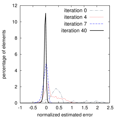
(a)

(b)

Figure 4: Left: distribution of the error over elements. Middle: standard deviation of error distribution. Right: Distribution of the local effectivity. The global effectivity index is indicated by a red star for the coarse uniform mesh, by a blue square for the fine uniform mesh, and a black plus for the adapted mesh.

Next we assess the performance of the algorithm towards equidistributing the error. The distribution of the estimated error for different iterations is plotted in Figure 4. The error is normalized by taking $e_{K}=\log_{10}\left(\frac{\eta_{K}}{TOL/\sqrt{N_{T}}}\right)$. From the figure, we see that after successive iterations the error increasingly tends to cluster towards the target error and the distribution tends to be more normal. Furthermore, the standard deviation of the error decreases from $0.58$ on the initial mesh to $0.041$ on the final mesh.

Next we establish numerically the equivalence between the exact and estimated error. The motivation is to assess to what degree we can expect to control the exact error, both locally and globally, by equidistributing the estimated error as in Figure 4. Define the global effectivity index with respect to the energy norm by $ei=\frac{\eta}{{\left|\kern-0.75346pt\left|\kern-0.75346pt\left|e_{h}\right|\kern-0.75346pt\right|\kern-0.75346pt\right|}},$ where $\eta=\sqrt{\sum_{K}\eta_{K}^{2}}.$ Theorem 1 says that globally the energy norm of the error is equivalent to the estimated error, so that the effectivity index assesses this equivalence on a given mesh. Ideally, the effectivity index satisfies $ei\rightarrow 1$ as the mesh element size goes to $0$, in which case we say that the estimator is asymptotically exact. This effectivity index is studied for instance in [32] and [28], where it was observed to remain reasonably low for adapted meshes (between 2 to 5). Furthermore, for meshes adapted with target error $TOL$, the index remains bounded as $TOL\rightarrow 0$, see for instance [32, Table 3.7]. Thus, while the estimator is not asymptotically exact, it is clearly equivalent to the exact error.

We define the local effectivity index for a triangle $K$ by

$$ei_{K}=\frac{\eta_{K}}{|e_{h}|_{1,K}}.$$ (23)

(Recall that since $A=I$ in (1) the energy norm is just the $H^{1}$ seminorm.) The quantity (23) measures the equivalence of the exact and estimated error at the level of the element. In Figure 4 we plotted the distribution of (23) for a few meshes. For the coarse uniform mesh with $200$ elements, note that while the global effectivity index is quite low ($ei=1.08$), the distribution of the local effectivity index is spread out, with a large upper tail. On the other hand, the finer uniform mesh with $20000$ elements has a higher global effectivity index ($ei=1.70$) with a smaller tail, suggesting that the accuracy of the estimator improves with refinement. We also show the distribution for a relatively coarse adapted mesh with $4500$ elements. While the global effectivity index is higher ($ei=2.42$), the local effectivity index is more closely distributed about the global effectivity index. What appears to happen is that refinement exaggerates the overestimation of the error that already occurs in uniform meshes.

Control of the $L^{2}$ norm of the error.

In the remainder of the subsection, we will assess numerically the lower and upper bounds for the $L^{2}$ error given in (22), and briefly present some results using the estimator (14) for mesh adaptation.

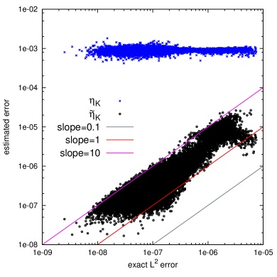
(a) Estimated error (5) and (14) vs. the exact $L^{2}$ error for a mesh adapted using the original estimator (5).

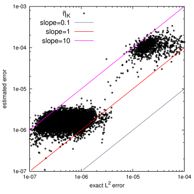
(b) Estimated error (14) vs. the exact $L^{2}$ error for two meshes adapted using the scaled estimator (14).

Figure 5: Estimated error vs. exact $L^{2}$ error over elements.

Setting $TOL=0.125$, the final adapted mesh using $\eta_{K}$ mesh has about $18000$ elements. Figure 5a records for each element the estimated error $\eta_{K}$ (in blue) and $\tilde{\eta}_{K}$ (in black) vs. the exact $L^{2}$ error $\|e_{h}\|_{0,K}$. While $\eta_{K}$ remains within less than $1$ order of magnitude, the exact $L^{2}$ error is spread by about $3$ orders. Therefore, equidistributing the estimator $\eta_{K}$ does not lead to equidistribution of the $L^{2}$ error. In verifying the lower and upper from (22), we see that the local effectivity index $\tilde{ei}_{K}=\frac{\tilde{\eta}_{K}}{\|e_{h}\|_{0,K}}$ remains between about $0.1$ and $10,$ with the lower bound appearing sharp.

Next we adapt the mesh using the scaled error $\tilde{\eta}_{K}$. The mesh is adapted using the hybrid error approach from [5] for the hierarchical estimator. That is, edge refinement and node removal are used to control the global $L^{2}$ error level (here using (14)), while edge swapping and node movement are used to equidistribute the error by minimizing the energy norm (here using (5)). Results of two meshes adapted using different target error levels are presented in Figure 5b: a mesh with about $1000$ elements (top right) and one with $14000$ (bottom left). The spread of the $L^{2}$ error is significantly lower, going from $3$ orders of magnitude to about $1.5$.

(a)

(b)

Figure 6: Energy norm (left) and $L^{2}$ norm (right) error calculations for $u_{1}$ for residual estimators.

We compare global error calculations using the scaled and non-scaled estimator in Figure 6. Clearly, the non-scaled estimator results in lower energy norm error for the same degrees of freedom. Moreover, as predicted, the scaled error significantly improves the results for the $L^{2}$ error.

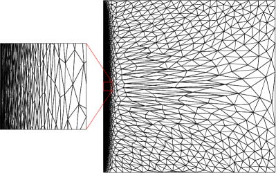
(a)

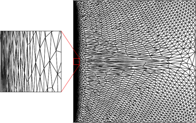
(b)

Figure 7: Adapted meshes with $2500$ vertices using the $H^{1}$ estimator (left) and scaled estimator (right).

Lastly, we compare meshes adapted with the scaled and unscaled estimators in Figure 7. Both meshes have roughly the same number of vertices/elements, but the distribution of the elements for the mesh adapted using the scaled estimator is much more spread throughout the domain, while that in the original estimator tends to concentrate near the boundary $x=0.$ This observation is really not surprising, since scaling the estimator by the smallest eigenvalue will permit elements to be larger in areas where the $H^{1}$ error is largest, such as the boundary layer. Generally, we expect that the error converges at a higher order in the $L^{2}$ norm than for the $H^{1}$ seminorm error. But as seen in Figure 5b, this higher order is not just global (at the level of the domain), but local (element level). This observation about mesh quality being related to the norm will be further confirmed in what follows when we consider the hierarchical estimator, which natively controls the $L^{2}$ error.

4.1.2 Comparison of the adaptation methods

Qualitative comparison.

Figure 8 presents examples of adapted meshes with about $2500$ vertices produced by each method. In all cases, we see that the meshes contain elements that are very stretched near the boundary layer. Note that in general the meshes obtained from the residual estimators tend to have more elements near the boundary layer, while the meshes from Hessian and hierarchical methods tends to be more spread out. The difference in mesh density is likely due to the target norm used by each method. As discussed in the previous section, the target norm is related to the local order of convergence, which affects local element size.

Another note is that the mesh for the Hessian is quite regular in the top and bottom right corners. The initial mesh is regular, consisting of right triangles as in Figure 2a, so what seems to be happening is that in these regions the main operation performed is edge refinement. In particular, node displacement appears to be less smooth for the Hessian. Repeating the adaptation loop starting from a non-uniform mesh does in fact result in a final mesh which is not regular.

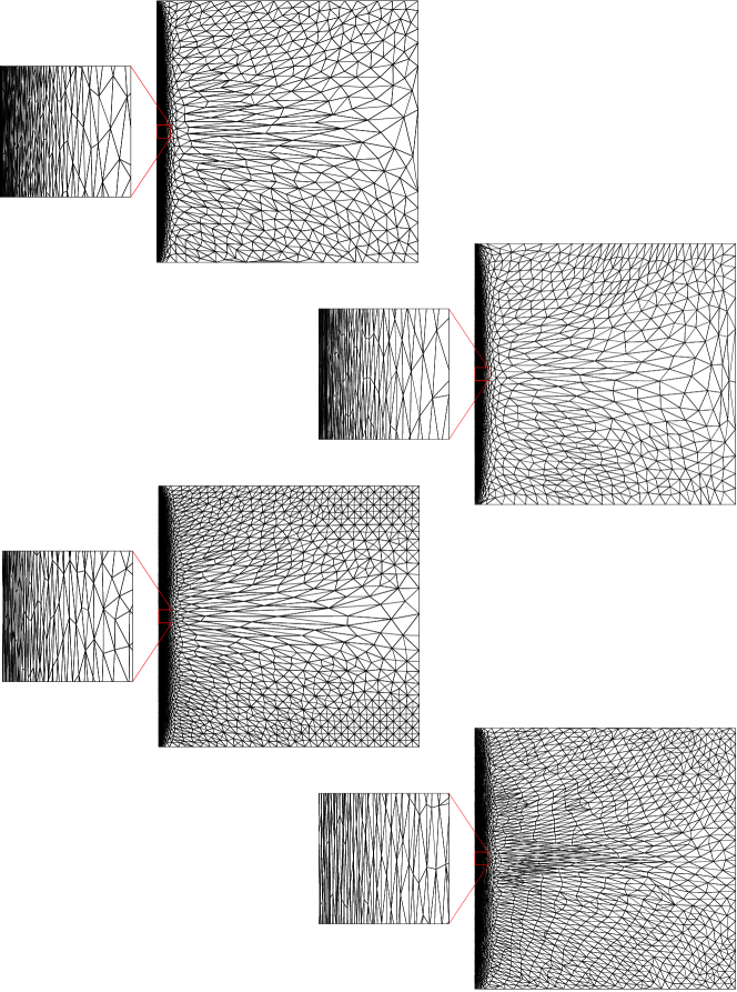
Figure 8: Adapted meshes for $u_{1}$ with approximately 2500 vertices, with zoom near the boundary at $x=0$. From top to bottom: residual (element), residual (metric), Hessian, hierarchical.

Analytical comparison.

The error is reported in Figure 9 as a function of the number of vertices. Recall that for a regular mesh in $2D$, the number of vertices is roughly proportional to $(\frac{1}{h})^{2}$, so that the theoretically optimal (logarithmic) slope corresponding to (11) is $-1/2$, while for (13) it is $-1$.

Figure 9 reports the error in the energy and $L^{2}$ norm. We see that all methods approach the theoretical rate of convergence for the energy norm. Moreover the hierarchical method, which reports the largest error, remains about $1.3$ times higher than the residual element-based method, which reports the smallest error. The convergence for the $L^{2}$ norm, on the other hand, appears to be more erratic, with none of the methods achieving the optimal rate of convergence. Here the hierarchical method reports the lowest error, the residual methods report an error $2$ to $3$ times as large, while the Hessian method reports an error about $4$ to $5$ times as large. Note that for both, the energy and $L^{2}$ norms, the results for both residual methods are close.

(a)

(b)

Figure 9: Energy norm (left) and $L^{2}$ norm (right) error calculations for $u_{1}$.

In Table 2 we record the mean and variance of the distribution of the error over the elements. While Figure 9 shows that the global energy norm is lowest for the residual methods and highest for the hierarchical, the situation is reversed here, with the hierarchical reporting the lowest mean error. This can be partially accounted for by the fact that the residual methods result in the lowest standard deviation for the energy norm of the error, which is likely the result of the equidistribution of the estimated error achieved by the adaptive method. For the $L^{2}$ error, as expected the hierarchical method reports the lowest mean and standard deviation.

We remark that the target norm for the Hessian adaptation is $L^{\infty},$ so it is possible that the Hessian does the best job equidistributing the error in the $L^{\infty}$ norm. We did not calculate the $L^{\infty}$ norm. Furthermore, it should be noted that in [26], a Hessian-based error estimator was developed to control the the $L^{p}$ error for $1\leq p<\infty.$ Adaptation is, as before, done by constructing a metric, which turns out to be the the same as that discussed in Section 3.5 with the eigenvalues appropriately scaled for the choice of $p$, see [26, Section 2]. It is reasonable to expect that the results for the $L^{2}$ error could be improved using their estimates.

method	vertices	mean	st. dev.	mean	st. dev.
		$\|\nabla(e_{h})\|_{K}$	$\|\nabla(e_{h})\|_{K}$	$\|e_{h}\|_{K}$	$\|e_{h}\|_{K}$
residual (element)	657	5.37e-03	1.20e-03	2.16e-05	3.16e-05
residual (metric)	639	6.04e-03	1.74e-03	2.63e-05	3.93e-05
Hessian	691	5.27e-03	3.84e-03	2.27e-05	2.07e-05
hierarchical	670	5.42e-03	5.30e-03	1.84e-05	1.21e-05
residual (element)	2369	1.42e-03	2.82e-04	3.25e-06	5.13e-06
residual (metric)	2251	1.62e-03	4.09e-04	3.55e-06	4.99e-06
Hessian	2342	1.51e-03	1.08e-03	4.40e-06	5.98e-06
hierarchical	2356	1.41e-03	1.54e-03	2.14e-06	1.08e-06
residual (element)	8992	3.63e-04	7.24e-05	4.51e-07	7.65e-07
residual (metric)	8701	4.01e-04	8.88e-05	4.99e-07	8.20e-07
Hessian	8842	3.85e-04	2.56e-04	6.63e-07	1.09e-06
hierarchical	8786	3.55e-04	3.62e-04	2.96e-07	1.72e-07
residual (element)	35218	9.12e-05	1.76e-05	7.13e-08	1.44e-07
residual (metric)	33448	1.02e-04	2.14e-05	8.16e-08	1.58e-07
Hessian	38290	8.78e-05	7.92e-05	1.06e-07	1.85e-07
hierarchical	38205	7.90e-05	8.10e-05	3.95e-08	2.97e-08

Table 2: Distribution of error.

Computational performance.

Figure 10a records the CPU time for the adaptation part of each iteration of the loop. For each method, we chose the global error level so that the final mesh has about $9000$ vertices. The number of vertices at each iteration is recorded in Figure 10b, and the gap between lowest and highest at the last step is about $6$%. We find that metric adaptation requires much less time than the other methods, and in the plot both metric based methods appear superimposed. This result is not surprising. The only that value we really need to keep track of is the metric tensor at each vertex. The local error calculations are relatively insubstantial compared to those required for element-based adaptation.

In addition, note that the element-based residual method takes roughly $5$ to $6$ times that of the hierarchical estimator. For one thing, the residual estimator requires the contribution from discontinuous functions. These functions cannot be directly interpolated after performing local modifications, and must be recomputed on each element/edge. Especially problematic is the calculation of the singular value decomposition. Even for a $2\times 2$ matrix $A$, it can be numerically disastrous to calculate the singular value decomposition of $A$ directly by first computing $AA^{T}$ [20], and instead it is recommended to use an iterative method. We have used the implementation provided by DGESVD from LAPACK. Overall, it was found that this computation takes between $13-18$% of the total adaptation process. Another contribution towards increased CPU time is due to the fact that the jump term depends on more than one element. As mentioned in Section 3.1.2, when performing edge swapping, the error needs to be calculated on an enlarged patch as in Figure 1 in order to accurately compute the jump term. The construction and handling of this patch introduces significant computational overhead.

(a) CPU-time in seconds

(b) Number of nodes

Figure 10: Left: CPU time for each iteration. Right: number of nodes at each iteration.

4.2 Second test case

With the same parameters for problem (1) as test case 1, we consider the function taken from [30]

$$u_{2}=\tan^{-1}(\alpha(r-r_{0})),$$

where $r=\sqrt{(x+0.05)^{2}+(y+0.05)^{2}},$ and $r_{0}=0.7$. Thus, we have a circular a wave-front type solution, centered at $(-0.05,-0.05)$ with a transition region with thickness of order $\alpha^{-1}.$ We will run simulations with both $\alpha=100$ and $\alpha=1000.$

4.2.1 Qualitative comparison

In Figures 11 we show some examples of adapted meshes. In each case, the mesh follows what we would expect from the solution. The elements are mainly concentrated near the wave-front where the gradient is steep in the direction orthogonal to the wave, and with the alignment of the elements in this region reflecting the curvature. Outside this region, variation in the solution is reduced significantly, so that the elements can be much larger. What is striking, however, is the difference between the mesh produced by the hierarchical method compared to the others. For the hierarchical method, the mesh is more spread out and less concentrated near the wave-front. As discussed in Section 4.1, we attribute this difference to the target norm used. Another feature of interest, seen in the zoom to the wave-front, is a sub-layer of elements where the mesh is coarser. In this region, the function is almost linear in the direction orthogonal to the wave-front, so that the error is somewhat smaller than in the immediate surroundings.

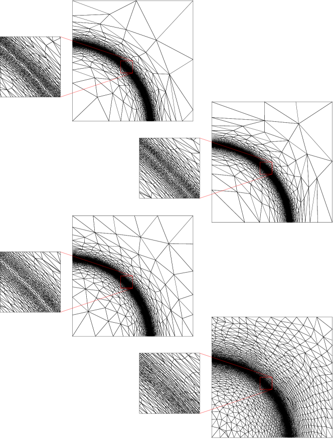
Figure 11: Adapted meshes for $u_{2}$, $\alpha=100$ with approximately 3000 vertices, with zoom to wave front. From top to bottom: residual (element), residual (metric), Hessian, hierarchical.

4.2.2 Analytical comparison

Calculation of the residual term.

This test case highlights one of the drawbacks of residual estimators. To calculate the error $\eta_{K}$, we need to evaluate the integrals $\int_{K}f^{2}\,\,\mathrm{d}x$ of the source term $f.$ (Since $A=I$ and $u_{h}$ is piecewise linear, we get $R_{K}(u_{h})=f$.) At the wave front with $\alpha=1000$ this value is very difficult to compute accurately. The immediate effect on adaptation was that some elements were not being refined despite being flagged as having large error. In particular, the algorithm reported

$$\int_{K_{1}}f^{2}\,\,\mathrm{d}x+\int_{K_{2}}f^{2}\,\,\mathrm{d}x \gg\int_{K}f^{2}\,\,\mathrm{d}x,$$ (24)

where $K_{1},\,K_{2}$ are obtained by refining an edge of $K.$

We improve the accuracy of the integral by subdivision. For a given quadrature rule $\mathcal{Q}_{K}$ on an element, we divide the triangle into $4$ by splitting the edges in half, then define the subdivided quadrature rule $\mathcal{Q}_{K,1}$ to be that composed of four copies of the original, each weighted $\frac{1}{4}|K|.$ The effect is that if the rule we had before was $Ch^{k}$ accurate, the subdivided scheme is $\frac{C}{2^{k}}h^{k}$ accurate. We therefore increase the accuracy without introducing a large constant from a higher-order method. See Algorithm 2 for implementation details.

Algorithm 2 Calculation of the residual on element $K$.

1. Calculate the residual $\tilde{R}_{0}$ with the original quadrature $\mathcal{Q}_{K,0}$.

2. Choose $\epsilon>0$ to be small. For $i=0,1,2$ do the following:

   1. Subdivide the current quadrature $\mathcal{Q}_{K,i}$ into $\mathcal{Q}_{K,i+1}$ and compute the residual $\tilde{R}_{i+1}.$

   2. If $i=2$ or if $\frac{|\tilde{R}_{i}-\tilde{R}_{i+1}|}{\tilde{R}_{i+1}}\leq\epsilon$ then accept $\tilde{R}_{i+1}$ as the residual and exit.

Since each time we subdivide, we multiply the number of Gauss points by $4$, subdivision can quickly become expensive. We always subdivide at least once, so that at the very least we need to compute values at $(1+4)B_{G}$ points, where $B_{G}$ is the base number of Gauss points. Therefore, higher-order quadrature rules are virtually unusable for subdivision, and the total number of subdivisions never exceeds $3$. Fortunately, in our case it was sufficient to use the single point (barycenter) integration scheme. Even still, this comes at the high cost of $64$ Gauss points for the third subdivision. The percentage of subdivisions that occur for an adaptation loop with $\epsilon$ from Algorithm 2 set to $0.05$ are reported Figure 3. By the tenth iteration, additional subdivision is not significant.

it.	2 sub. %	3 sub. %
1	7.55	4.02
5	10.69	2.69
10	1.79	0.88
20	1.49	0.77

Table 3: Percentage of elements where additional subdivision occurs at each iteration of the global adaptation step.

We remark that subdivision integration is not necessary if adapting using a metric. There, the residual is calculated only once to compute the metric so that issues such as (24) will not be seen during adaptation. Furthermore, when computing the metric, the residual term is often left out altogether to save computational time, as is done in [9]. Theoretically, this simplification can be justified for the Laplace equation as proven in [23]. In the case of element-based adaptation, we found that including the residual term was necessary, since experiments with removing the residual term generally resulted in meshes of poor quality.

Global error comparison.

In Figures 12 and 13, we record the error convergence for $u_{2}$ for $\alpha=100$ and $\alpha=1000$. The results are very similar to that for $u_{1}$: for the energy norm, the results are close, with the element-based residual method reporting the lowest error, while for the $L^{2}$ error, as in Section 4.1, the hierarchical method reports the lowest. The results for the $L^{2}$ error for $\alpha=1000$ will be discussed in some detail here, for they clearly highlight the issue of controlling the $L^{2}$ norm with an estimator for the $H^{1}$ seminorm. We found that the $L^{2}$ error oscillates over consecutive iterations when adapting with the residual in some situations. To illustrate this issue, we reported the results in a different way in Figure 13. For each target error, after the number of local modifications and vertices has stabilized, we take the smallest and largest error after $10$ further adaptation iterations, giving an upper and lower envelope. With the exception of the residual element-based, where we see a persistent spread of about $5$ to $10$%, the envelope becomes narrow as the number of nodes increases.

(a)

(b)

Figure 12: Energy norm error calculations for $u_{2}$ with $\alpha=100$ (left) and $\alpha=1000$ (right).

(a)

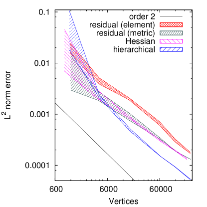
(b)

Figure 13: $L^{2}$ norm error calculations for $u_{2}$ with $\alpha=100$ (left) and $\alpha=1000$ (right). The plot on the right depicts the envelope of the oscillating error.

In Figure 14, we illustrate that the oscillation is due to a few outlier elements, appearing just before and after the wave-front. These elements account for a significant percentage of the overall error, and at each iteration, slight variations in this region cause significant fluctuation in the error. From the Figure 13b we see that for coarse meshes, this instability arises for all methods. For the hierarchical method, as we decrease the target error, the region is refined, and the $L^{2}$ error stabilizes. The lack of stability for the $L^{2}$ error in the case of the residual estimator is the result of two combined factors. First, the estimator does not detect the fact that the $L^{2}$ error is still quite large outside the wave-front, and therefore, even at very fine meshes of over $250000$ vertices, the mesh is not refined in those regions. This observation fits within the context of Proposition 1 very well, because while we have equidistributed the $H^{1}$ seminorm error over the elements, the value of $\lambda_{2,K}$ is much smaller for elements at the wave-front, which predicts that the $L^{2}$ error should also be much lower. The other contributing factor is that the mesh is not completely stationary in this region, so that slight variations in the mesh, which barely registered as far as the $H^{1}$ seminorm is concerned, cause large variations in the $L^{2}$ error.

(a)

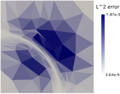
(b)

Figure 14: Mesh with about $1100$ vertices adapted with the hierarchical method (left) and the distribution of the exact $L^{2}$ error (right).

5 Conclusion

We introduced an element-based mesh adaptation method for the anisotropic a posteriori error estimator appearing in [32]. The method is done by interfacing with the hierarchical estimator driver from MEF++, as introduced in [5]. We tested the method in numerical test cases that feature significant anisotropic behaviour and verified that the adaptation algorithm produces anisotropic meshes and converges. Additionally, we considered an $L^{2}$ norm error variant of the estimator, which, under some hypotheses on the mesh, is equivalent to the exact $L^{2}$ error. Numerical examples were provided to confirm the equivalence with the exact error. Examples of adapted meshes using the modified estimator were provided, and it was found to give improved performance for control of the $L^{2}$ error over the original estimator.

The new element-based method was compared with three existing anisotropic mesh adaptation methods for $P_{1}$ finite elements: residual metric based, Hessian metric, and hierarchical. In terms of controlling the level of error with respect to degree of freedom, the new method generally performed slightly better for the energy norm, while the hierarchical method performed significantly better than the other methods for the $L^{2}$ norm. However, the new method is significantly more expensive from a computational standpoint. We note that the results for both element and metric based methods for the residual estimator were generally very close for both norms. Given the results presented in Section 4, it seems likely that the method that obtains a given level of error in the energy norm in the shortest time would be the residual metric method, while for $L^{2}$ error it would be one of the residual metric or Hessian methods.

Currently the authors are working on optimizing the computational aspects of the method to make it more competitive with the other methods in terms of CPU efficiency. Additionally, an investigation is being made to determine why the element residual cannot be dropped from the computation, as for instance in [9].

References

- [1] M. Ainsworth and J.T. Oden. A posteriori error estimation in finite element analysis. Comput. Methods Appl. Mech. Engrg., 142:1–88, 1997.
- [2] I. Babuska and W. Rheinboldt. Error estimates for adaptive finite element method computations. Int. J. Numer. Methods Engrg., 12:1597–1615, 1978.
- [3] I. Babuska and W. Rheinboldt. A posteriori error estimatimates for the finite element method. Int. J. Numer. Methods Engrg., 12:1597–1615, 1978.
- [4] Y. Belhamadia, A. Fortin, and E. Chamberland. Anisotropic mesh adaptation for the solution of the stefan problem. J. Comput. Phys., 194(1):233–255, 2004.
- [5] R. Bois, M. Fortin, and A. Fortin. A fully anisotropic mesh adaptation method based on a hierarchical error estimator. Comput. Methods Appl. Mech. Engrg., 209-212:12–27, 2012.
- [6] Richard Bois. Adaptation de maillages anisotropes par un estimateur d’erreur hierarchique. PhD thesis, Universite Laval, 2012.
- [7] H. Borouchaki, P. George, F. Hecht, P. Laug, and E. Saltel. Delaunay mesh generation governed by metric specifications. Part I. Algorithms. Finite Elem. Anal. Des., 25(1-2):61–83, 1997.
- [8] Y. Bourgault, M. Picasso, F. Alauzet, and A. Loseille. On the use of anisotropic a posteriori error estimates for the adaptative solution of 3D inviscid compressible flows. Int. J. Numer. Meth. Fluids, 59:47–74, 2009.
- [9] E. Burman and M. Picasso. Anisotropic, adaptive finite elements for the computation of a solutal dentrite. Interfaces and Free Boundaries, 5:103–127, 2003.
- [10] C. Carstensen and R. Verfürth. Edge residuals dominate a posteriori error estimates for low order finite element methods. SIAM J. Numer. Anal., 27:1571–1587, 1999.
- [11] Franco Dassi, Simona Perotto, and Luca Formaggia. A priori anisotropic mesh adaptation on implicitly defined surfaces. SIAM J. Sci. Comput., 37(6):A2758–A2782, 2015.
- [12] E. D’Azevedo. Optimal triangular mesh generation by coordinate transformation. SIAM J. Sci. Stat. Comput., 12(4):755–786, 1991.
- [13] E. D’Azevedo and R. Simpson. On optimal interpolation triangle incidences. SIAM J. Sci. Stat. Comput., 10(6):1063–1075, 1989.
- [14] C. Dobrzynski. Adaptation de maillage anisotrope 3D et application à l’aéro-thermique des bâtiments. PhD thesis, Université Pierre et Marie Curie, 2005.
- [15] L. Formaggia and S. Perotto. New anisotropic a priori error estimates. Numer. Math., 89:641–667, 2001.
- [16] L. Formaggia and S. Perotto. Anisotropic error estimates for elliptic problems. Numer. Math., 94:67–92, 2003.
- [17] P. Frey and P.L. George. Mesh Generation: Application to Finite Elements. Wiley, Hoboken, NJ, 2nd edition, 2008.
- [18] P.L. George. Gamanic3d, adaptive anisotropic tetrahedral mesh generator. Technical note, INRIA, Paris, 2003.
- [19] GIREF. http://giref.ulaval.ca/.
- [20] G. Golub and C. Van Loan. Matrix Computations. Johns Hopkins Studies in the Mathematical Sciences. Johns Hopkins University Press, Baltimore, MD, 3rd edition, 1996.
- [21] W. Habashi, J. Dompierre, Y. Bourgault, D. Ait-Ali-Yahia, M. Fortin, and M. Vallet. Anisotropic mesh adaptation: towards user-independent, mesh-independent and solver-independent cfd. part I: General principles. Int. J. Numer. Meth. Fluids, 32:725–744, 2000.
- [22] F. Hecht. BAMG: Bidimensional anisotropic mesh generator. http://www.ann.jussieu.fr/hecht/ftp/bamg/bamg.pdf.
- [23] G. Kunert and R. Verfürth. Edge residuals dominate a posteriori error estimates for linear finite element methods on anisotropic triangular and tetrahedral meshes. Numer. Math., 86(2):283–303, 2000.
- [24] P. Laug and H. Bourochaki. BL2D-V2 : mailleur bidimensionnel adaptatif. Technical Report RT-0275, INRIA, Paris, 2003.
- [25] A. Loseille and F. Alauzet. Continuous mesh framework part I: Well-posed continuous interpolation error. SIAM J. Numer. Anal., 49(1):38–60, 2011.
- [26] A. Loseille and F. Alauzet. Continuous mesh framework part II: Validations and applications. SIAM J. Numer. Anal., 49(1):61–86, 2011.
- [27] A. Lozinski, M. Picasso, and V. Prachittham. An anisotropic error estimator for the Crank-Nicolson method: applications to a parabolic problem. SIAM J. Sci. Comput., 31(4):2757–2783, 2009.
- [28] S. Micheletti and S. Perotto. Reliability and efficiency of an anisotropic Zienkiewicz-Zhu error estimator. Comput. Methods Appl. Mech. Engrg., 195:799–835, 2006.
- [29] Stefano Micheletti, Simona Perotto, and Marco Picasso. Stabilized finite elements on anisotropic meshes: a priori error estimates for the advection-diffusion and the Stokes problems. SIAM J. Numer. Anal., 41(3):1131–1162 (electronic), 2003.
- [30] W. Mitchell. A collection of 2D elliptic problems for testing adaptive algorithms. Technical report, NISTIR 7668, 2010.
- [31] J Pascal. A fully automatic adaptive isotropic surface remeshing procedure. 2001.
- [32] M. Picasso. An anisotropic error indicator based on Zienkiewicz-Zhu error estimator: Application to elliptic and parabolic problems. SIAM J. Sci. Comput., 24(4):1328–1355, 2003.
- [33] M. Picasso. Adaptive finite elements with large aspect ratio based on an anisotropic error estimator involving first order derivatives. Comput. Methods Appl. Mech. Engrg., 916:14–23, 2006.
- [34] A. Quarteroni and A. Valli. Numerical Approximation of Partial Differential Equations. Number 23 in Springer Series in Computational Mathematics. Springer-Verlag, 1997.
- [35] R. Rodriguez. Some remarks on Zienkiewicz-Zhu estimator. Numer. Methods Partial Different. Equat., 10:625–635, 1994.
- [36] Z. Zhang and A. Naga. A new finite element gradient recovery method: Superconvergence property. SIAM J. Sci. Comput., 26(4):1192–1213, 2005.