Information Measures, Inequalities and Performance Bounds for Parameter Estimation in Impulsive Noise Environments

Abstract

Recent studies found that many channels are affected by additive noise that is impulsive in nature and is best explained by heavy-tailed symmetric alpha-stable distributions. Dealing with impulsive noise environments comes with an added complexity with respect to the standard Gaussian environment: the alpha-stable probability density functions do not possess closed-form expressions except in few special cases. Furthermore, they have an infinite second moment and the “nice” Hilbert space structure of the space of random variables having a finite second moment –which represents the universe in which the Gaussian theory is applicable, is lost along with its tools and methodologies.

This is indeed the case in estimation theory where classical tools to quantify the performance of an estimator are tightly related to the assumption of having finite variance variables. In alpha-stable environments, expressions such as the mean square error and the Cramer-Rao bound are hence problematic.

In this work, we tackle the parameter estimation problem in impulsive noise environments and develop novel tools that are tailored to the alpha-stable and heavy-tailed noise environments, tools that coincide with the standard ones adopted in the Gaussian setup; namely a generalized “power” measure and a generalized Fisher information. We generalize known information inequalities commonly used in the Gaussian context: the de Bruijn’s identity, the data processing inequality, the Fisher information inequality, the isoperimetric inequality for entropies and the Cramer-Rao bound. Additionally, we derive upper bounds on the differential entropy of independent sums having a stable component. Intermediately, the new power measure is used to shed some light on the additive alpha-stable noise channel capacity in a setup that generalizes the linear average power constrained AWGN channel. Our theoretical findings are paralleled with numerical evaluations of various quantities and bounds using developed Matlab packages.

Keywords: Impulsive noise, alpha-stable, power, estimation, Fisher information, Fisher information inequality, Cramer-Rao bound, differential entropy of sums, upper bounds, de Bruijn’s identity, isoperimetric inequality.

I Introduction

The presence of impulsive-noise such as those with alpha-stable statistics, is rather frequent in communications theory. Indeed, interference has been often found to be of impulsive nature and is best explained by alpha-stable distributions. This is the case for telephone noise [1] and audio noise signals [2]. Furthermore, in many works that treated the multiuser interference in radio communication networks, a theoretical derivation, based on the assumption that the interferers are distributed over the entire plane and behave statistically as a Point Poisson Process (PPP), yielded an interference with alpha-stable statistics, starting with Sousa [3] who computed the self interference, considering only the pathloss effect for three spread spectrum schemes, direct sequence with binary phase shift keying (DS/BPSK), frequency hopping with M-ary frequency shift keying (FH/MFSK), and frequency hopping with on-off keying (FH/OOK), where a sinusoidal tone is transmitted as the “on” symbol. In [4], the authors introduced a novel approach to stable noise modeling based on the LePage series representation which permits the extension of the results on multiple access communications to environments with lognormal shadowing and Rayleigh fading. Continuous time multiuser interference was also found [5] to be well represented as an impulsive alpha-stable random process. Recently in [6], alpha-stable distributions were found to model well the aggregate interference in wireless networks: the authors treated the problem in a general framework that accounts for all the essential physical parameters that affect network interference with applications in cognitive radio, wireless packets, covert military schemes and networks where narrowband and ultra-wide band systems coexist. In [7], Gulati et al. showed that the statistical-physical modeling of co-channel interference in a field of Poisson and Poisson-Poisson clustered interferers obeys an alpha-stable or Middleton class A statistics depending whether the interferers are spread in the entire plane, in a finite area or in a finite area with a guard zone with the alpha-stable being suitable for wireless sensor, ad-hoc and femtocells networks when both in-cell and out-of-cell interference are included. A generalization of the previous results for radio frequency interference in multiple antennas is found in [8] where joint statistical-physical interference from uncoordinated interfering sources is derived without any assumption on spatial independence or spatial isotropic interference. Lastly, the alpha-stable model arises as a suitable noise model in molecular communications [9].

An important problem in the theory of non-random parameter estimation is to find “good” estimators of some quantity of interest based on a given observation. Generally, this is done by using a quality measure of the estimator’s (average) performance: the Mean Square Error (MSE). The use of the MSE is tightly related to the assumption of finite variance noise and one can even argue that it is related to a “potential Gaussian” setup. Naturally, under this finite-variance assumption, one can restrict the quest of finding “good” estimators to the Hilbert space of finite second moment Random Variables (RV)s which leads to the well-established “Gaussian” or “linear” estimation theory. When the observation is contaminated with an impulsive noise perturbation –having an infinite variance, restricting the look-up universe for good estimators to that of finite variance RVs is no longer optimal neither necessarily sensible. Additionally, tools such as the MSE will turn out to be problematic.

In this work we consider the non-random parameter estimation problem whereby we want to estimate a non-random parameter(s) $\theta\in\mathbb{R}\,(\mathbb{R}^{d})$ based on a noisy observation $X=\theta+N$ and where the additive noise $N$ is of impulsive nature. In the case where the noise $N$ has a finite variance, the problem is well-understood: let $\hat{\theta}(X)$ be an estimator of $\theta$ based on observing $X$, then

• The quality of the estimator is measured via the MSE: “$\,\textsf{E}\left[{\left|\hat{\theta}(X)-\theta\right|^{2}}\right]$”. Hence, Minimum Mean Square Error (MMSE) estimators are optimal.

• A lower-bound on the MSE of the estimator is given by the Cramer-Rao (CR) bound:

  $$\textsf{E}\left[{\left|\hat{\theta}(X)-\theta\right|^{2}}\right]\geq\frac{1}{J(N)},$$ (1)

  where $J(N)$ is the Fisher information of the RV $N$.

• Equality holds in equation (1) whenever $N$ is Gaussian distributed and $\hat{\theta}(X)=X$ is the Maximum Likelihood (ML) estimator.

In order to understand the parameter estimation problem in the impulsive noise scenario, one must answer the following:

• Under the impulsive noise assumption, the MMSE estimator is not necessarily optimal and the linear MSE estimator is not sensible. “Good” estimators candidates might possibly have an infinite second moment which implies that a new quality measure has to be defined. This quality measure is to be interpreted as the average “strength” or power of the estimation error.

• Since the Fisher information $J(\cdot)$ is tightly related to Gaussian variables through de Bruijn’s identity, a new information measure has to be defined– one that is adapted to impulsive noise variables. Similarly to $J(\cdot)$, the new information measure is to be related to the alpha-stable distribution through a de Bruijn’s type of equality.

• Establishing a new CR bound: the new quality measure of an estimator is to be lower bounded, function of the inverse of the new information measure.

When it comes to objective 1, a survey of the literature shows that few alternative measures of power were proposed:

• In [10], Shao and Nikias proposed the “dispersion” of a RV as a measure that plays a similar role to the variance. However, since no analytical expression is defined for the dispersion except for alpha-stable distributions, they propose the usage of the Fractional Lower Order Moments (FLOM) $\textsf{E}\left[{|X|^{r}}\right]$ ($r<2$) as an alternative which yields a non-linear signal processing theory.

• Based on logarithmic moments of the form $\textsf{E}\left[{\log|X|}\right]$, an alternative notion of power was introduced by Gonzales [11] for heavy-tailed distributions which he labeled as the Geometric Power (GP):

  $$\mathcal{S}_{0}(X)\;\hat{=}\;e^{\textsf{E}\left[{\log|X|}\right]}.$$

  The author considered logarithmic moments as a “universal framework” for dealing with algebraic tail processes that will overcome the shortcomings of the FLOM approach which he summarized by the fact that no appropriate value of $r$ is feasible for all impulsive processes. Also the discontinuity in the FLOM is yet another unpleasant feature. In fact, for a given $0<r<2$, two alpha stable distributions with characteristic exponents $\alpha_{1}=r+\epsilon$ and $\alpha_{2}=r-\epsilon$ (for some $\epsilon>0$), will respectively have a finite and infinite $r$-th absolute moment, though one can agree that they would have similar statistical behavior. However, all stable distributions have a finite logarithmic moment [11].

The GP was used in formulating new impulsive signal processing techniques with the proposition of new types of non-linear filters referred to as “myriad filters”, which are basically Maximum Likelihood (ML) estimators of the location of a Cauchy distribution with an optimality tune parameter [12]. However, the GP suffers from a serious drawback since for any variable $X$ that has a mass point at zero, $\mathcal{S}_{0}(X)$ will be necessarily null even if say other non-zero mass points are existent. This would yield a zero power for a non-zero signal.

In relation to objective 2, generalizing “Gaussian” information-theoretic properties and tools to “stable” ones is done in [13] where a new score function is defined in terms of a scaled conditional expectation and a de Bruijn’s identity is found in terms of the new score function in a relative manner with respect to that of a stable variable. Recently in [14], Toscani proposed a fractional score function using fractional derivatives and defined a fractional Fisher information that evaluates to infinity for stable variables. Using it in a relative manner –with respect to stable variables, the relative fractional Fisher information is found to satisfy a Fisher information inequality and is used to find the rate of convergence in relative entropy of scaled Independent and Identically Distributed (IID) sums to stable variables.

Up to the authors’ knowledge, objective 3 has only been addressed in [15] where the authors derived a Cramer-Rao type of inequality featuring the finite fractional moment of order $r\geq 1$ of a variable and a generalized Fisher information. The work in [15] was in the direction of extending information theoretic inequalities to new ones where generalized Gaussians are extremal distributions rather than characterizing the quality of estimators in impulsive noise environments. We also note that the CR result in [15] suffers from the restriction of having variables with finite fractional moments of order $r\geq 1$ which is not the case in this paper where variables with only finite logarithmic moments are considered.

Naturally, this parameter estimation problem is also that of estimating the location parameter of an alpha-stable variable. Previous works that treated the estimation of the various parameters of alpha-stable distribution [16, 17, 18, 19, 20, 21, 22] had a primary goal of finding specific estimators. They are based on heuristics for which the authors either conducted consistency or asymptotic analysis, or tested empirical evaluations versus numerical computations and Monte-Carlo simulations in order to validate and evaluate the proposed estimators. In this context, in this work we define and find quality measures and universal bounds that are satisfied by all location parameter estimators of impulsive distributions. Our main contributions are four fold:

1. A generalized power notion: The evaluation of performance measures in multiple applications in communications theory is generally done function of the channel state quality. A key quantity that summarizes the quality of the channel is the Signal-to-Noise Ratio (SNR) which is a ratio between the power of a signal containing the relevant information to that of the noise signal. A standard measure of the signal power is made through the evaluation of the second moment. When working in alpha-stable noise environments, some information bearing signals will necessarily have an infinite second moment which eventually leads to having zero SNRs, a fact that masks the possibility to quantify the channel’s state. We propose in Definition 1 a new “relative” power measure that we call the $\alpha$-power ​: a strength measure that takes into account the type of the disturbing noise. This would seem reasonable whenever the goal of the communication system is to maintain a Quality of Service (QoS) level for some or all of its users which is translated, for example, to a threshold rate (output entropy) or an output SNR. In both cases the QoS will be dependent on the output signal. Our “output”-based approach is tailored to this type of applications since it focuses on the output signal and takes into account the type of the encountered noise in the received signal in order to define sensible tools to quantify the QoS criteria. As an example, we derive in Theorem 2 the capacity of an additive stable noise channel under a constraint on its output’s $\alpha$-power .

   Another application is the parameter estimation problem where the observed output, affected by stable noise is sufficient for the characterization of the estimator’s performance. The generalized power measure is chosen in such a way that when constraining it, stable variables will be entropy maximizers, proven in Theorem 1. It is then shown to comply with generic properties that are satisfied by the standard deviation and is numerically evaluated for different types of probability densities.

2. A generalized information measure: We consider an alternative formulation of the Fisher information that is more relevant than $J(X)$ when dealing with RVs corrupted by additive noise of infinite second moment; In essence, our starting point is one where –in a similar fashion to the Gaussian case– we enforce a generalized de Bruijn identity to hold: motivated by the fact that the derivative of the differential entropy with respect to small variations in the direction of a Gaussian variable is a scaled $J(\cdot)$, we propose in Definition 2 a new notion of Fisher information as a derivative of differential entropy in the direction of infinitesimal perturbations along stable variables and we label it the “Fisher information of order $\alpha$” or the $\alpha$-Fisher information ​​. Next, we derive in Lemma 1 an integral expression for the new quantity that is a generalization of the well-known expression of the Fisher information. We note that the definition of the $\alpha$-Fisher information in this manuscript is an absolute measure and different from the one in [14]. It has different usages and applications and was independently developed.

3. Generalized information-theoretic inequalities: Information inequalities have been investigated since the foundation of information theory. It started with Shannon [23] with the fact that Gaussian distributions maximize entropy under a second moment constraint. Then a lower bound on the entropy of independent sums of RVs, commonly known as the Entropy Power Inequality (EPI) was proved. The EPI states that given two real independent RVs $X$, $Z$ such that $h(X)$, $h(Z)$ and $h(X+Z)$ exist, then (Corollary 3, [24])

   $$N(X+Z)\geq N(X)+N(Z),$$ (3)

   where $N\left(X\right)$ is the entropy power of $X$ and is equal to

   $$N\left(X\right)=\frac{1}{2\pi e}e^{2h(X)}.$$

   The EPI was a proposition of Shannon who provided a local proof. Later Stam [25] followed by Blachman [26] presented complete proofs. These proofs of the EPI relied on two information identities: the de Bruijn’s identity and the Fisher Information Inequality (FII). The latter states that given $X$ and $Z$ two independent RVs such that the respective Fisher information $J(X)$ and $J(Z)$ exist. Then

   $$\frac{1}{J(X+Z)}\geq\frac{1}{J(X)}+\frac{1}{J(Z)}.$$ (4)

   The remarkable similarity between  equations (3) and (4) was pointed out in Stam’s paper [25] who in addition, related the entropy power and the Fisher information by an “uncertainty principle-type” relation:

   $$N(X)J(X)\geq 1,$$ (5)

   which is commonly known as the Isoperimetric Inequality for Entropies (IIE) [27, Theorem 16]. Interestingly, equality holds in equation (5) whenever $X$ is Gaussian distributed and in equations (3)–(4) whenever $X$ and $Z$ are independent Gaussians. As it can be noticed, the previously cited inequalities revolve around Gaussian variables. When it comes to the general stable family, the relative fractional Fisher information defined in [14] is found to satisfy a Fisher information inequality and is used to find the rate of convergence in relative entropy of scaled IID sums to stable variables. In this paper, we generalize these information theoretic inequalities that are based on the Gaussian setting to generic ones in the stable setting which coincide with the regular identities in the Gaussian setup. Namely, when restricted to the range $1<\alpha\leq 2$, the $\alpha$-Fisher information is found in Theorem 7 to satisfy a Generalized Fisher Information Inequality (GFII). Then, we use the GFII and the generalized de Bruijn (proven in Theorem 4) to derive in Theorem 8 an upper bound on the differential entropy of the independent sum of two RVs where one of them is stable. Finally, in Theorem 9 a Generalized Isoperimetric Inequality for Entropies (GIIE) is proved to hold.

4. A Generalized Cramer-Rao bound: Well-known identities such as the Cramer-Rao bound which provides a lower bound on the mean square error of estimators in the from of the inverse of $J(X)$ are adequate in the finite variance setup. If the observed noisy variable has an infinite second moment, the use of the Cramer-Rao bound in its classical form is problematic. We derive in Theorem 10 a generalized Cramer-Rao bound, that relates the “relative” power of the estimation error to the generalized Fisher information $J_{\alpha}(\cdot)$.

The rest of this paper is organized as follows: we propose in Section II the $\alpha$-power , a generalized power parameter and we provide some of its properties and applications. We define in Section III the $\alpha$-Fisher information , we list its properties and we establish a generalized de Bruijn’s identity. In Section IV, information inequalities are shown to be satisfied by the the $\alpha$-Fisher information with applications in finding upper bounds on the differential entropy of independent sums when one of the variables is stable and establishing a generalized IIE. The generalized CR bound is stated and proved in Section V and Section VI concludes the paper.

II The $\alpha$-power ​, a Relative Power Measure

Power measures are important tools that can provide partial yet fundamental information about a signal. They serve multiple purposes such as signal strength comparisons or as reference units for the computation of performance and quality indicators. We stipulate that a “strength” or power measure $\text{P}\left({\mathbf{X}}\right)$ of a random vector $\mathbf{X}$ should satisfy the following:

• $\text{P}\left({\mathbf{X}}\right)\geq 0$, with equality if and only if ${\bf X}=0$.

• $\text{P}\left({a\mathbf{X}}\right)=|a|\text{P}\left({\mathbf{X}}\right)$, for all $a\in\mathbb{R}$.

These restrictions are “minimal” and do not contain for example some of the dispensable properties satisfied by the GP such as the multiplicativity and the triangular inequality properties [11]. However they are deemed sufficient to define a strength measure.

As a notion of average power, the second moment is the answer to a widely known result in communications theory; it is the constraint under which a Gaussian density function is entropy maximizer. In order to come up with a notion of average power in the presence of alpha-stable distributions, one might consider adopting the measure/constraint under which sub-Gaussian  symmetric alpha-stable  (S$\alpha$S ) density functions with an underlying Gaussian vector having IID zero-mean components (refer to Definition 5, Appendix A) are entropy maximizers; an approach that we adopt in what follows.

II-A A Power Parameter in the Presence of Stable Variables

In this manuscript we denote by $\tilde{\mathbf{Z}}_{\alpha}\!\sim\bm{\mathcal{S}}\left(\alpha,\left(\frac{1}{\alpha}\right)^{\frac{1}{\alpha}}\right)$ a reference Symmetric Stable (SS) vector, i.e.,

• whenever $\alpha\neq 2$: a reference sub-Gaussian S$\alpha$S vector with an underlying Gaussian vector having IID zero-mean components with variance $\sigma^{2}=2\left(\frac{1}{\alpha}\right)^{\frac{2}{\alpha}}$.

• when $\alpha=2$: a reference Gaussian vector of IID components with mean zero and variance 1.

Definition 1 (Power Parameter).

The “power of order $\alpha$” or $\alpha$-power of non-zero random vector $\mathbf{X}$ is the non-negative scalar $\text{P}_{\!\alpha\!}\left({\mathbf{X}}\right)$ such that:

$$-\textsf{E}\left[{\ln p_{{\bf\tilde{Z}_{\alpha}\!}}\left(\frac{{\mathbf{X}}}{\text{P}_{\!\alpha\!}\left({\mathbf{X}}\right)}\right)}\right]=h(\tilde{\mathbf{Z}}_{\alpha}\!),$$ (6)

where $h(\tilde{\mathbf{Z}}_{\alpha}\!)$ is the differential entropy of $\tilde{\mathbf{Z}}_{\alpha}\!\,$. For the deterministic $\mathbf{X}={\bf 0}$, we define $\text{P}_{\!\alpha\!}\left({\mathbf{X}}\right)=0$.

The existence and uniqueness of the $\alpha$-power will be addressed shortly. Intuitively, one may think of $\text{P}_{\!\alpha\!}\left({\mathbf{X}}\right)$ as a “relative power” with respect to $\tilde{\mathbf{Z}}_{\alpha}\!$ which is a reference variable whose $\alpha$-power is equal to unity. In the two special cases where closed-form expression of the PDF is available, the $\alpha$-power can be evaluated:

• When $\alpha=2$, $\tilde{\mathbf{Z}}_{2}\!$ is a zero-mean Gaussian vector with identity covariance matrix and

  $$\text{P}_{\!2\!}\left({\mathbf{X}}\right)=\sqrt{\frac{\textsf{E}\left[{\|\mathbf{X}\|^{2}}\right]}{d}}.$$

• When $\alpha=1$ (see [28]),

  $$p_{{\bf\tilde{Z}_{1}\!}}(\mathbf{x})=\frac{1}{\pi^{\frac{d+1}{2}}}\Gamma\left(\frac{d+1}{2}\right)\,\frac{1}{\left(1+\|\mathbf{x}\|^{2}\right)^{\frac{d+1}{2}}},$$

  and $\text{P}_{\!1\!}\left({\mathbf{X}}\right)$ is the solution of

  $$\textsf{E}\left[{\ln\left(1+\left\|\frac{\mathbf{X}}{\text{P}_{\!1\!}\left({\mathbf{X}}\right)}\right\|^{2}\right)}\right]=\textsf{E}\left[{\ln\left(1+\left\|\tilde{\mathbf{Z}}_{1}\!\right\|^{2}\right)}\right].$$

As defined in (6), the quantity $\text{P}_{\!\alpha\!}\left({\mathbf{X}}\right)$ is endowed with some power properties that we list hereafter and prove in Appendix B.

Property 1.

Let $\mathbf{X}$ and $\mathbf{Y}$ be random vectors such that:

$$\left\{\begin{array}[]{ll}\textsf{E}\left[{\ln\left(1+\|\mathbf{X}\|\right)}\right]<\infty,&\text{ when considering cases where }\alpha<2.\\ \textsf{E}\left[{\|\mathbf{X}\|^{2}}\right]<\infty&\text{ when considering cases where }\alpha=2.\end{array}\right.$$

The following properties hold:

• The $\alpha$-power $\text{P}_{\!\alpha\!}\left({\mathbf{X}}\right)$ exists, is unique and $\text{P}_{\!\alpha\!}\left({\mathbf{X}}\right)\geq 0$ with equality if and only if $\mathbf{X}={\bf 0}$.

• For any $a\in\mathbb{R},\text{P}_{\!\alpha\!}\left({a\mathbf{X}}\right)=|a|\,\text{P}_{\!\alpha\!}\left({\mathbf{X}}\right)$.

• If $\mathbf{X}$ and $\mathbf{Y}$ are independent and $\mathbf{Y}$ has a rotationally symmetric PDF that is non-increasing in $\|\mathbf{y}\|$, then $\text{P}_{\!\alpha\!}\left({\mathbf{X}+\mathbf{Y}}\right)\geq\text{P}_{\!\alpha\!}\left({\mathbf{Y}}\right)$.

• If $\mathbf{X}$ and $\mathbf{Y}$ are independent and $\mathbf{Y}$ has a rotationally symmetric PDF that is non-increasing in $\|\mathbf{y}\|$, then $\text{P}_{\!\alpha\!}\left({c\mathbf{X}+\mathbf{Y}}\right)$ is non-decreasing in $|c|$, $c\in\mathbb{R}$.

• Whenever $\mathbf{X}\sim\bm{\mathcal{S}}\left(\alpha,\gamma_{\mathbf{X}}\right)$, $\text{P}_{\!\alpha\!}\left({\mathbf{X}}\right)=(\alpha)^{\frac{1}{\alpha}}\gamma_{\mathbf{X}}$.

Though the definition of the $\alpha$-power as stated in equation (6) is implicit and dependent on the density function of the SS vector ${\bf\tilde{Z}_{\alpha}\!}$ which does not have closed form expression except in the special cases of the Cauchy and the Gaussian distributions, the computation of the $\alpha$-power $\text{P}_{\!\alpha\!}\left({\mathbf{X}}\right)$ of a certain random vector $\mathbf{X}$ can be done efficiently using numerical computations. In fact, the stable densities can be computed numerically as inverse Fourier transforms or by using Matlab packages that compute these densities such as the “Stable” package provided by Nolan [29]. We use here the latter and we develop a Matlab code that computes the $\alpha$-power for a scalar RV according to Definition 1. We plot in Figure 1, the $\alpha$-power of several probability laws– Gaussian, uniform, Laplace, Cauchy and alpha-stable, with respect to a multitude of symmetric alpha-stable distributions with the characteristic exponent $\alpha$ ranging from $0.4$ to $1.8$.

• Consider for example $\tilde{Z}_{1.2\,}\!$. The $\alpha$-power of a Gaussian variable $X\sim\mathcal{N}(0,2)$ is equal to $\text{P}_{\!{1.2}\!}\left({X}\right)=0.7869$. Using the scalability property (ii), the $\alpha$-power of a Gaussian variable $X\sim\mathcal{N}(0,\sigma^{2})$ is equal to $\text{P}_{\!{1.2}\!}\left({X}\right)=0.7869\frac{\sigma}{\sqrt{2}}=0.5564\,\sigma$. Note that as already known, the power the Gaussian variable $X\sim\mathcal{N}(0,\sigma^{2})$ with respect to $\tilde{Z}_{2}\!\sim\mathcal{N}(0,1)$ is equal to $\text{P}_{\!2\!}\left({X}\right)=\sigma$.

• Another example is when $X\sim\mathcal{U}[-a,+a]$, a uniform RV with zero mean and variance equal to $\frac{a^{2}}{3}$. With respect to $\tilde{Z}_{0.8}\!$, it has an $\alpha$-power of $\text{P}_{\!{\;0.8}\!}\left({X}\right)=0.3036\frac{a}{\sqrt{3}}=0.1753\,a$, whereas with respect to the Gaussian law the power is equal to the standard deviation $\text{P}_{\!2\!}\left({X}\right)=\frac{a}{\sqrt{3}}=0.5774\,a$.

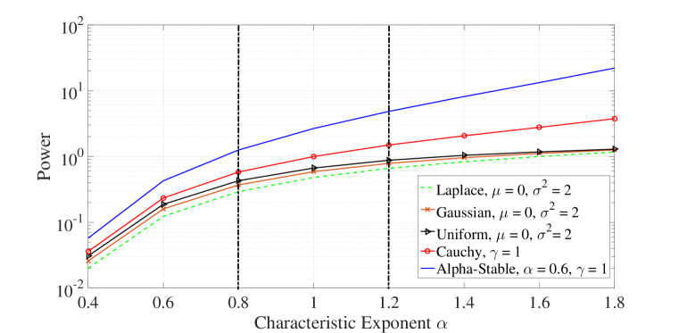
Figure 1: Evaluation of the $\alpha$-power of some probability laws with respect to $\tilde{Z}_{\alpha}\!\sim\mathcal{S}\left(\alpha,(\alpha)^{-\frac{1}{\alpha}}\right)$ for different values of $\alpha$.

For the value of the exponent $\alpha=2$, the $\alpha$-power of the Cauchy and alpha-stable laws evaluate to infinity and they are not shown in Figure 1.

II-B Applications

The new “power” measure may be used in a variety of setups. We showcase in what follows two scenarios related to two fundamental information-theoretic problems: entropy maximization and channel capacity evaluation.

II-B1 Stable Maximizing Entropy

Having adopted a generic power definition when considering stable noise environments, we study the solution of the entropy maximization problem subject to a constraint on the newly defined power. Namely, let $\text{P}>0$ and consider the set of random variables whose $\alpha$-power is equal to P:

$$\mathcal{P}=\left\{\text{distribution functions}\,\,F\,\,\text{on}\,\,\mathbb{R}^{d}:-\int\ln p_{\bf\tilde{Z}_{\alpha}\!}\left(\frac{\bf x}{\text{P}}\right)\,dF(\mathbf{x})=h({\bf\tilde{Z}_{\alpha}\!})\right\}.$$

According to [30, Section 12.1], among all distribution functions $F\in\mathcal{P}$, the one that maximizes differential entropy has the following PDF:

$$p^{*}(\mathbf{x})=e^{\lambda_{0}+\lambda_{1}\ln p_{\bf\tilde{Z}_{\alpha}\!}\left(\frac{\bf x}{\text{P}}\right)}=e^{\lambda_{0}}p_{\bf\tilde{Z}_{\alpha}\!}^{\lambda_{1}}\left(\frac{\bf x}{\text{P}}\right),$$

where $\lambda_{0}$ and $\lambda_{1}$ are chosen so that $p^{*}(\mathbf{x})\in\mathcal{P}$. Since $\frac{1}{\text{P}}\,p_{\bf\tilde{Z}_{\alpha}\!}\left(\frac{\bf x}{\text{P}}\right)$ is of the sought after form,

$$\arg\max_{F\in\mathcal{P}}\,h(F)=\text{P}{\bf\tilde{Z}_{\alpha}\!}\sim\bm{\mathcal{S}}\left(\alpha,\left(\frac{1}{\alpha}\right)^{\frac{1}{\alpha}}\text{P}\right),$$ (7)

and the value of the maximum is:

$$h(F^{*})=h({\bf\tilde{Z}_{\alpha}\!})+d\ln\text{P}.$$

As a direct generalization, one can write:

Theorem 1.

Let

$$\mathcal{P}_{A}=\left\{\text{distribution functions}\,\,F\,\,\text{on}\,\,\mathbb{R}^{d}:0<\text{P}_{\!\alpha\!}\left({F}\right)\leq A,\,A>0\right\}.$$ (8)

Then

$$A{\bf\tilde{Z}_{\alpha}\!}=\arg\max_{F\in\mathcal{P}_{A}}\,h(F),$$

and the maximum entropy value is $h({\bf\tilde{Z}_{\alpha}\!})+d\ln A$ .

II-B2 Communicating over Stable Channels

Consider the additive linear channel:

$$\mathbf{Y}=\mathbf{X}+\mathbf{N},$$ (9)

where $\mathbf{Y}$ is the channel output, $\mathbf{X}$ is the input and $\mathbf{N}\sim\bm{\mathcal{S}}\left(\alpha,\gamma_{\bf N}\right)$ is the additive SS noise vector which is independent of $\mathbf{X}$. We ask the following question: what constraint is to be imposed on the input such that a stable input achieves the capacity of channel (9)? Under this scenario, and knowing that a stable input generates a stable output, a sufficient condition is that the output space induced by the channel is the space where a stable variable maximizes entropy, specifically a space of a form as in (8). This leads to the following result:

Theorem 2.

Let $\mathbf{N}\sim\bm{\mathcal{S}}\left(\alpha,\gamma_{\bf N}\right)$ and $A$ be a non-negative scalar such that $A\geq\text{P}_{\!\alpha\!}\left({\mathbf{N}}\right)=(\alpha)^{\frac{1}{\alpha}}\gamma_{\bf N}$. Consider the space $\mathcal{P}_{\left[\text{P}_{\!\alpha\!}\left({\mathbf{N}}\right),A\right]}$ of probability distributions:

$$\mathcal{P}_{\left[\text{P}_{\!\alpha\!}\left({\mathbf{N}}\right),A\right]}=\left\{\text{distribution functions}\,\,F\,\,\text{on}\,\,\mathbb{R}^{d}:\text{P}_{\!\alpha\!}\left({\mathbf{N}}\right)\leq\text{P}_{\!\alpha\!}\left({F}\right)\leq A\right\}.$$ (10)

Whenever the output $\mathbf{Y}$ of channel (9) is subjected to (10), the channel capacity evaluates to:

$$C=d\ln\left(\frac{A}{\text{P}_{\!\alpha\!}\left({\mathbf{N}}\right)}\right)=d\ln\left(\text{SNR}_{\text{output}}\right),$$

and is achieved by $\mathbf{X}^{*}\sim\bm{\mathcal{S}}\left(\alpha,\left(\frac{1}{\alpha}\right)^{\frac{1}{\alpha}}\sqrt[\alpha]{A^{\alpha}-\text{P}_{\!\alpha\!}\left({\mathbf{N}}\right)^{\alpha}}\right)$. Furthermore, the input cost constraint can be written as:

$$\exists\,\text{P}\in\left[\text{P}_{\!\alpha\!}\left({\mathbf{N}}\right),A\right],\qquad\textsf{E}_{\mathbf{X}}\left[{D\left(p_{\text{P}_{\!\alpha\!}\left({\mathbf{N}}\right){\bf\tilde{Z}_{\alpha}\!}}(\mathbf{v}-\mathbf{X})\big{\|}p_{\text{P}{\bf\tilde{Z}_{\alpha}\!}}({\bf v})\right)}\right]=\ln\frac{\text{P}}{\text{P}_{\!\alpha\!}\left({\mathbf{N}}\right)}.$$ (11)

Proof:

By Theorem 1, under condition (10) a stable output $\mathbf{Y}^{*}\sim\bm{\mathcal{S}}\left(\alpha,\left(\frac{1}{\alpha}\right)^{\frac{1}{\alpha}}A\right)$ maximizes the output entropy and achieves the channel capacity $C$:

$$C=h(\mathbf{Y}^{*})-h(\mathbf{N}) = d\ln(A)+h({\bf\tilde{Z}_{\alpha}\!})-d\ln(\text{P}_{\!\alpha\!}\left({\mathbf{N}}\right))-h({\bf\tilde{Z}_{\alpha}\!})$$

$$= d\ln\left(\frac{A}{\text{P}_{\!\alpha\!}\left({\mathbf{N}}\right)}\right),$$

where we used the fact that $h(\mathbf{N})=\ln(\text{P}_{\!\alpha\!}\left({\mathbf{N}}\right))+h({\bf\tilde{Z}_{\alpha}\!})$ since $\gamma_{\bf N}=\text{P}_{\!\alpha\!}\left({\mathbf{N}}\right)\gamma_{\bf\tilde{Z}_{\alpha}\!}$. The optimal input $\mathbf{X}^{*}$ which yields $\mathbf{Y}^{*}$ is also distributed according to a stable variable with parameter $\gamma_{\mathbf{X}^{*}}$:

$$\gamma^{\alpha}_{\mathbf{X}^{*}}=\gamma^{\alpha}_{\mathbf{Y}^{*}}-\gamma^{\alpha}_{\mathbf{N}}=\frac{1}{\alpha}\left(A^{\alpha}-\text{P}_{\!\alpha\!}\left({\mathbf{N}}\right)^{\alpha}\right),$$

which by property (v) yields,

$$\text{P}_{\!\alpha\!}\left({\mathbf{X}^{*}}\right)^{\alpha}=\alpha\gamma^{\alpha}_{\mathbf{X}^{*}}=A^{\alpha}-\text{P}_{\!\alpha\!}\left({\mathbf{N}}\right)^{\alpha}.$$

Finally, we determine below the input cost constraint that yields the output space $\mathcal{P}_{\left[\text{P}_{\!\alpha\!}\left({\mathbf{N}}\right),A\right]}$. The output condition (10) is explicitly stated as the space of all random vectors $\mathbf{Y}$ such that there exists a $\text{P}>0$, such that $\text{P}_{\!\alpha\!}\left({\mathbf{N}}\right)\leq\text{P}\leq A$ and

$$-\textsf{E}\left[{\ln p_{\bf\tilde{Z}_{\alpha}\!}\left(\frac{\mathbf{Y}}{P}\right)}\right]=h({\bf\tilde{Z}_{\alpha}\!})\quad\iff\quad\textsf{E}_{\mathbf{X}}\left[{-\textsf{E}_{\mathbf{N}}\left[{\ln p_{\bf\tilde{Z}_{\alpha}\!}\left(\frac{\mathbf{X}+\mathbf{N}}{P}\right)\Bigg{|}\mathbf{X}}\right]}\right]=h({\bf\tilde{Z}_{\alpha}\!}),$$ (12)

where we used the iterated expectations to write the second equation. Equation (12) can be interpreted as the input cost function $\mathcal{C}(\cdot)$ being

$$\mathcal{C}\left(\mathbf{x},\text{P}\right)=-\textsf{E}_{\mathbf{N}}\left[{\ln p_{\bf\tilde{Z}_{\alpha}\!}\left(\frac{\mathbf{x}+\mathbf{N}}{P}\right)}\right],$$ (13)

and the input cost constraint being:

$$\exists\,\text{P}\in\left[\text{P}_{\!\alpha\!}\left({\mathbf{N}}\right),A\right],\qquad\textsf{E}_{\mathbf{X}}\left[{\mathcal{C}\left(\mathbf{X},\text{P}\right)}\right]=h({\bf\tilde{Z}_{\alpha}\!}).$$

The cost function and the cost constraint can be written in a different form:

$$\mathcal{C}(\mathbf{x},\text{P}) = -\int p_{\text{P}_{\!\alpha\!}\left({\mathbf{N}}\right){\bf\tilde{Z}_{\alpha}\!}}(\mathbf{n})\,\ln p_{\bf\tilde{Z}_{\alpha}\!}\left(\frac{\mathbf{x}+\mathbf{n}}{P}\right)\,d\mathbf{n}$$ (14)

$$= -\int p_{\text{P}_{\!\alpha\!}\left({\mathbf{N}}\right){\bf\tilde{Z}_{\alpha}\!}}\left(\mathbf{v}-\mathbf{x}\right)\,\ln\left(\frac{1}{\text{P}}p_{\bf\tilde{Z}_{\alpha}\!}\left(\frac{\mathbf{v}}{\text{P}}\right)\right)\,d\mathbf{v}-\ln\text{P}$$

$$= -\int p_{\text{P}_{\!\alpha\!}\left({\mathbf{N}}\right){\bf\tilde{Z}_{\alpha}\!}}(\mathbf{v}-\mathbf{x})\,\ln p_{\text{P}{\bf\tilde{Z}_{\alpha}\!}}(\mathbf{v})\,d\mathbf{v}-\ln\text{P}$$

$$= D\left(p_{\text{P}_{\!\alpha\!}\left({\mathbf{N}}\right){\bf\tilde{Z}_{\alpha}\!}}(\mathbf{v}-\mathbf{x})\big{\|}p_{\text{P}{\bf\tilde{Z}_{\alpha}\!}}(\mathbf{v})\right)+h(\text{P}_{\!\alpha\!}\left({\mathbf{N}}\right){\bf\tilde{Z}_{\alpha}\!})-\ln\text{P}$$

$$= D\left(p_{\text{P}_{\!\alpha\!}\left({\mathbf{N}}\right){\bf\tilde{Z}_{\alpha}\!}}(\mathbf{v}-\mathbf{x})\big{\|}p_{\text{P}{\bf\tilde{Z}_{\alpha}\!}}(\mathbf{v})\right)+h({\bf\tilde{Z}_{\alpha}\!})+\ln\frac{\text{P}_{\!\alpha\!}\left({\mathbf{N}}\right)}{\text{P}},$$

where $D(p\|q)$ is the Kullback-Leibler divergence between two PDFs $p$ and $q$. Using equation (14), the input cost constraint can be rewritten as:

$$\textsf{E}_{\mathbf{X}}\left[{D\left(p_{\text{P}_{\!\alpha\!}\left({\mathbf{N}}\right){\bf\tilde{Z}_{\alpha}\!}}(\mathbf{v}-\mathbf{X})\big{\|}p_{\text{P}{\bf\tilde{Z}_{\alpha}\!}}({\bf v})\right)}\right]=\ln\frac{\text{P}}{\text{P}_{\!\alpha\!}\left({\mathbf{N}}\right)}.$$

∎

Note that the capacity problem at hand of the stable channel (9) under the input cost constraint (11) is a generalization to the well known AWGN channel under the average power constraint [23] and the additive independent Cauchy channel under a logarithmic constraint [31].

Finally, in the scalar case the generic cost function $\mathcal{C}(x)$ presented in (13) is $\Theta(x^{2})$ when $\alpha=2$. For all other values of $\alpha$, using the same methodology as in [32] one can prove that $\mathcal{C}(x)=\Theta\left(\ln|x|\right)$ by virtue of the fact that $\ln p_{\tilde{Z}_{\alpha}\!}(x)=\Theta(\ln|x|)$. This comes in accordance with the results presented in [32].

II-C Extensions and Insights

The $\alpha$-power measure $\text{P}_{\!\alpha\!}\left({\mathbf{X}}\right)$ defined in (6) is related to a choice of ${\bf\tilde{Z}_{\alpha}\!}$ –or equivalently a choice of $0<\alpha\leq 2$, and as previously mentioned $\text{P}_{\!\alpha\!}\left({\mathbf{X}}\right)$ can be looked at as the relative power of $\mathbf{X}$ with respect to that of ${\bf\tilde{Z}_{\alpha}\!}$. Naturally one would ask the following: In a specific scenario, what value of alpha is more suitable? An answer to this question is given when considering, for example, an additive noise channel $\mathbf{Y}=\mathbf{X}+{\bf N}$. In fact, in most communications’ applications, the quantity of interest for a system engineer is the received signal or the output $\mathbf{Y}$ as it generally represents the quantity that will undergo further processing in order to retrieve the useful information. In addition, the noise variable ${\bf N}$ imposed by the channel represents another important variable since relevant quantities and performance measures are computed function of the relative power between the output signal and the noise, a quantity that is commonly referred to as the output SNR. Moreover, the output $\mathbf{Y}$ is shaped by the noise ${\bf N}$, hence it has “similar” characteristics to those of ${\bf N}$ (for example, a vector ${\bf N}$ having infinite variance components will always induce a vector $\mathbf{Y}$ having infinite variance components). This is to say, that in the context of an additive stable noise channel, it would seem natural to measure the power of the different signals with respect to a reference stable variable whose power evaluates to unity. Hence the choice of $\alpha$ and then ${\bf\tilde{Z}_{\alpha}\!}$ becomes straightforward depending on the stable noise characteristic exponent $\alpha$.

A natural extension is to generalize the adoption of $\text{P}_{\!\alpha\!}\left({\mathbf{X}}\right)$ for a specific ${\bf\tilde{Z}_{\alpha}\!}$ to cases where the noise is not necessarily stable but falls instead in the domain of normal attraction $\mathbb{D}_{\alpha}$ [33, 34] of the stable variables. For example, in the scalar case, any noise variable having a finite second moment belongs to $\mathbb{D}_{2}$ and $\text{P}_{\!2\!}\left({X}\right)$ is equal to the second moment. For noise variables whose tail behavior is $\Theta\left(\frac{1}{|x|^{1+\alpha}}\right)$, $0<\alpha<2$, the $\alpha$-power $\text{P}_{\!\alpha\!}\left({X}\right)$ should be used.

III $\alpha$-Fisher information : A Generalized Information Measure

In this section, we introduce a family of new information measures $\left\{J_{\alpha}(\cdot)\right\}_{0<\alpha\leq 2}$ and its properties as a generalization of the standard Fisher information. This is done through enforcing a family of identities of the de Bruijn type and finding an analytical expression of $J_{\alpha}(\cdot)$, $0<\alpha\leq 2$.

Definition 2 ($\alpha$-Fisher information ).

Let $X$ be a finite differential entropy RV and $\tilde{Z}_{\alpha}\!$ an independent reference SS variable $\tilde{Z}_{\alpha}\!\sim\mathcal{S}\left(\alpha,\left(\frac{1}{\alpha}\right)^{\frac{1}{\alpha}}\right)$, $0<\alpha\leq 2$. We define the “Fisher information of order $\alpha$” or the $\alpha$-Fisher information $J_{\alpha}(X)$ as follows:

$$J_{\alpha}(X)=\alpha\cdot\lim_{\epsilon\rightarrow 0^{+}}\frac{h\left(X+\sqrt[\alpha]{\epsilon}\,\tilde{Z}_{\alpha}\!\right)-h(X)}{\epsilon},$$ (15)

whenever the limit exists.

For a $d$-dimensional random vector $\mathbf{X}=(X_{1},\cdots,X_{d})$, $J_{\alpha}(\mathbf{X})$ is defined as in (15) where $\tilde{\mathbf{Z}}_{\alpha}\!\sim\bm{\mathcal{S}}\left(\alpha,\left(\frac{1}{\alpha}\right)^{\frac{1}{\alpha}}\right)$ is the $d$-dimensional reference SS vector.

Alternatively, by the change of variable $t=\frac{\epsilon}{\alpha}$, if $N$ denotes an independent SS variable $N\sim\mathcal{S}\left(\alpha,1\right)$, the $\alpha$-Fisher information is

$$J_{\alpha}(X)=\lim_{t\rightarrow 0^{+}}\frac{h\left(X+\sqrt[\alpha]{t}\,N\right)-h(X)}{t},$$ (16)

whenever the limit exists. In the vector case, $J_{\alpha}(\mathbf{X})$ is also as in (16) where $\mathbf{N}\sim\bm{\mathcal{S}}\left(\alpha,1\right)$.

Before proceeding to discuss the properties of the newly defined quantity we point out that the existence of the limit is guaranteed in a wide range of scenarios:

Theorem 3.

For all random vectors $\mathbf{X}$ such that $\textsf{E}\left[{\ln\left(1+\|\mathbf{X}\|\right)}\right]$ and $h(\mathbf{X})$ are finite, $J_{\alpha}(\mathbf{X})$ exists for all $0<\alpha\leq 2$.

Proof:

We first note that $h(\mathbf{X}+\sqrt[\alpha]{t}\mathbf{N})$ exists and is finite since $\sqrt[\alpha]{t}\,\mathbf{N}\sim\bm{\mathcal{S}}\left(\alpha,\sqrt[\alpha]{t}\right)$ has a bounded PDF and $\textsf{E}\left[{\ln\left(1+\|\mathbf{X}\|\right)}\right]$ is finite [35, Proposition 1]. Also, in the scalar case it has been proven in [36] that the differential entropy $h(X+N_{t})$ is concave in $t\geq 0$ whenever $N$ is an infinitely divisible RV where $N_{t}$ is related to $N$ through their characteristic functions as follows [37, Theorem 2.3.9 p.65]:

$$\phi_{N_{t}}(\omega)=e^{t\ln\phi_{N}(\omega)}.$$

Since in our case the infinitely divisible RV is stable with characteristic exponent $\alpha$, then $N_{t}\sim\sqrt[\alpha]{t}N$ which implies that $h(X+N_{t})$ is concave in $t$ and therefore it is everywhere left and right differentiable and a.e differentiable. These properties generalize in a straightforward manner to the vector case, and hence $\frac{d}{dt}h(\mathbf{X}+\sqrt[\alpha]{t}\mathbf{N})$ exists a.e. in $t$ and $\frac{d}{dt}h(\mathbf{X}+\sqrt[\alpha]{t}\mathbf{N})\Big{|}_{t=0^{+}}$ exists. ∎

III-A Properties of the $\alpha$-Fisher information

Few properties of $J_{\alpha}(\mathbf{X})$ may be readily identified.

• It is non-negative: By definition, $J_{\alpha}(\mathbf{X})$ represents the rate of variation of $h(\mathbf{X})$ under a small disturbance in the direction of a standard SS vector. It represents the limit of positive quantities and therefore, $J_{\alpha}(\mathbf{X})\geq 0$.

• $J_{2}(\mathbf{X})$ coincides with the usual notion of Fisher information: When the stable noise $\mathbf{N}$ is Gaussian, i.e. $\alpha=2$, $J_{2}(\mathbf{X})$ coincides is the trace of the Fisher information matrix.

• It’s translation invariant: Let $\mathbf{c}\in\mathbb{R}^{d}$, then $J_{\alpha}(\mathbf{X}+\mathbf{c})=J_{\alpha}(\mathbf{X})$. This follows directly from the definition and from the translation invariant property of the differential entropy.

• It has a closed-form expression for symmetric stable vectors: If $\mathbf{X}\sim\bm{\mathcal{S}}\left(\alpha,\gamma\right)$ then $J_{\alpha}(\mathbf{X})=\frac{d}{\alpha}\frac{1}{\gamma^{\alpha}}$ nats. Indeed, if $\mathbf{X}\sim\bm{\mathcal{S}}\left(\alpha,\gamma\right)$ then $\mathbf{X}+\sqrt[\alpha]{\epsilon}\mathbf{N}\sim\bm{\mathcal{S}}\left(\alpha,\sqrt[\alpha]{\gamma^{\alpha}+\epsilon}\right)$ and

  $$J_{\alpha}(\mathbf{X}) = \lim_{\epsilon\rightarrow 0}\frac{h\left(\mathbf{X}+\sqrt[\alpha]{\epsilon}\mathbf{N}\right)-h(\mathbf{X})}{\epsilon}$$

  $$= \lim_{\epsilon\rightarrow 0}\frac{h\left(\sqrt[\alpha]{\gamma^{\alpha}+\epsilon}\mathbf{N}\right)-h(\gamma\mathbf{N})}{\epsilon}$$

  $$= \lim_{\epsilon\rightarrow 0}\frac{h\left(\mathbf{N}\right)+d\ln\left(\sqrt[\alpha]{1+\frac{\epsilon}{\gamma^{\alpha}}}\right)-h(\mathbf{N})}{\epsilon}$$

  $$= \frac{d}{\alpha}\frac{1}{\gamma^{\alpha}}\,\,\text{nats}.$$

  This result comes in accordance with the fact that $J_{2}(\mathbf{X})=J(\mathbf{X})=\frac{d}{\sigma^{2}}$ whenever $\mathbf{X}\sim\bm{\mathcal{N}}(0;\sigma^{2}\textsf{I})$ is Gaussian with covariance matrix $\sigma^{2}\textsf{I}$. This is true since in this case $\alpha=2$ and for a Gaussian variable $\gamma^{2}=\frac{\sigma^{2}}{2}$.

• Scales: $J_{\alpha}(a\mathbf{X})=\frac{1}{|a|^{\alpha}}J_{\alpha}(\mathbf{X})$ for $a\neq 0$. Indeed,

  $$J_{\alpha}(a\mathbf{X}) = \lim_{\epsilon\rightarrow 0}\frac{h\left(a\mathbf{X}+\sqrt[\alpha]{\epsilon}\mathbf{N}\right)-h(a\mathbf{X})}{\epsilon}$$

  $$= \lim_{\epsilon\rightarrow 0}\frac{h\left(\mathbf{X}+\sqrt[\alpha]{\frac{\epsilon}{|a|^{\alpha}}}\mathbf{N}\right)+d\ln|a|-h(\mathbf{X})-d\ln|a|}{\epsilon}$$

  $$= \frac{1}{|a|^{\alpha}}\lim_{\epsilon\rightarrow 0}\frac{h\left(\mathbf{X}+\sqrt[\alpha]{\frac{\epsilon}{|a|^{\alpha}}}\mathbf{N}\right)-h(\mathbf{X})}{\frac{\epsilon}{|a|^{\alpha}}}$$

  $$= \frac{1}{|a|^{\alpha}}J_{\alpha}(\mathbf{X}),$$

  where we used the fact that $(-\mathbf{N})$ is identically distributed as $\mathbf{N}$.

• Independent sums: $J_{\alpha}(\mathbf{X}+\mathbf{Z})\leq J_{\alpha}(\mathbf{X})$ when $\mathbf{Z}$ is independent of $\mathbf{X}$. Indeed

  $$J_{\alpha}(\mathbf{X}+\mathbf{Z}) =\lim_{t\rightarrow 0}\frac{h\left(\mathbf{X}+\mathbf{Z}+\sqrt[\alpha]{t}\mathbf{N}\right)-h(\mathbf{X}+\mathbf{Z})}{t}$$

  $$=\lim_{t\rightarrow 0}\frac{I(\mathbf{X}+\mathbf{Z}+\sqrt[\alpha]{t}\mathbf{N};\mathbf{N})}{t}$$

  $$\leq\lim_{t\rightarrow 0}\frac{I(\mathbf{X}+\sqrt[\alpha]{t}\mathbf{N};\mathbf{N})}{t}=J_{\alpha}(\mathbf{X}),$$

  where the inequality is due to the fact that $\mathbf{N}\mbox{ --- }\mathbf{X}+\sqrt[\alpha]{t}\mathbf{N}\mbox{ --- }\mathbf{X}+\mathbf{Z}+\sqrt[\alpha]{t}\mathbf{N}$ is a Markov chain.

• Sub-additivity: $J_{\alpha}(\cdot)$ is sub-additive for independent random vectors. Let $\mathbf{X}=\left(X_{1},\cdots,X_{d}\right)$ be a collection of $d$ independent RVs having Fisher information $\{J_{\alpha}(X_{i})\}_{i=1}^{d}$, then $J_{\alpha}(\mathbf{X})=J_{\alpha}(X_{1},\cdots,X_{d})\leq\sum_{i=1}^{d}J_{\alpha}(X_{i})$, because $h(Z_{1},\cdots,Z_{d})\leq\sum_{i=1}^{d}h(Z_{i})$ with equality whenever $\{Z_{i}\}_{i=1}^{d}$ are independent. It is known that $J_{2}(\cdot)$ is additive and it will be later shown that $J_{\alpha}(\cdot)$ is in fact additive.

Due to the above, one may consider $J_{\alpha}(\mathbf{X})$, $0<\alpha\leq 2$ as a measure of information. A single random vector $\mathbf{X}$ might hence have different information measures which represent from an estimation theory perspective a reasonable fact since the statistics of the additive noise $\mathbf{N}$ affect the estimation of $\mathbf{X}$ based on the observation of $\mathbf{X}+\mathbf{N}$. From this perspective, the original Fisher information would seem suitable when the adopted noise model is Gaussian or when we are restricting the RV to have a finite second moment.

III-B An expression of $J_{\alpha}(\cdot)$

We find in what follows an expression of $J_{\alpha}(\mathbf{X})$ whenever the random vector is absolutely continuous with a positive PDF. More precisely, let $\mathbf{X}\in\mathcal{V}$ where,

$$\mathcal{V}=\left\{\text{Absolutely continuous RVs }\mathbf{U}:p_{\mathbf{U}}(\mathbf{u})>0,h(\mathbf{U})\text{ is finite }\&\int\ln\left(1+\|\mathbf{U}\|\right)\,p_{\mathbf{U}}(\mathbf{u})\,d\mathbf{u}\text{ is finite }\right\}.$$

Lemma 1 (An Expression of the $\alpha$-Fisher information ).

Let $\mathbf{N}\sim\bm{\mathcal{S}}\left(\alpha,\gamma\right)$ be a SS vector and let $\mathbf{X}\in\mathcal{V}$ be independent of $\mathbf{N}$ with a characteristic function $\phi_{\mathbf{X}}(\bm{\omega})$ such that $\left[\|\bm{\omega}\|^{\alpha}\phi_{\mathbf{X}}(-\bm{\omega})\right]\in\text{L}^{1}(\mathbb{R}^{d})$. If there exists an $\epsilon>0$ such that

$$\bigg{\{}\Bigl{|}\ln p_{\mathbf{X}+\!\sqrt[\alpha]{t}\mathbf{N}}(\mathbf{x}){\mathcal{F}}_{\mathcal{I}}\bigl{[}\|\bm{\omega}\|^{\alpha}\phi_{\mathbf{X}+\!\sqrt[\alpha]{t}\mathbf{N}}(-\bm{\omega})\bigr{]}(\mathbf{x})\Bigr{|}\bigg{\}}_{t\in[0,\epsilon)}$$ (17)

are uniformly bounded in $t$ by an integrable function of $\mathbf{x}$, then the $\alpha$-Fisher information of $\mathbf{X}$ is

$$J_{\alpha}(\mathbf{X})=\int\ln p_{\mathbf{X}}(\mathbf{x})\,{\mathcal{F}}_{\mathcal{I}}\bigl{[}\|\bm{\omega}\|^{\alpha}\phi_{\mathbf{X}}(-\bm{\omega})\bigr{]}(\mathbf{x})\,d\mathbf{x}.$$ (18)

Proof:

Using Theorem 3 $J_{\alpha}(\mathbf{X})$ exists. Now, let $t\geq\eta\geq 0$ and denote $\mathbf{X}_{t}=\mathbf{X}+\sqrt[\alpha]{t}\mathbf{N}$ with characteristic function

$$\phi_{\mathbf{X}_{t}}(\bm{\omega}) =\phi_{\mathbf{X}}(\bm{\omega})\,e^{-t\gamma^{\alpha}\|\bm{\omega}\|^{\alpha}}\!\!=\phi_{\mathbf{X}_{\eta}}(\bm{\omega})\,e^{-(t-\eta)\gamma^{\alpha}\|\bm{\omega}\|^{\alpha}}$$

$$=\phi_{\mathbf{X}_{\eta}}(\bm{\omega})-(t-\eta)\gamma^{\alpha}\|\bm{\omega}\|^{\alpha}\phi_{\mathbf{X}_{\eta}}(\bm{\omega})+o(t-\eta).$$

By the linearity of the inverse Fourier transform,

$$p_{\mathbf{X}_{t}}\!(\mathbf{x})=p_{\mathbf{X}_{\eta}}\!(\mathbf{x})-(t-\eta)\gamma^{\alpha}{\mathcal{F}}_{\mathcal{I}}\bigl{[}\|\bm{\omega}\|^{\alpha}\phi_{\mathbf{X}_{\eta}}\!(-\bm{\omega})\bigr{]}(\mathbf{x})+o(t-\eta),$$ (19)

which is valid since the inverse distributional Fourier transform ${\mathcal{F}}_{\mathcal{I}}\bigl{[}\|\bm{\omega}\|^{m\alpha}\phi_{\mathbf{X}_{\eta}}(\bm{\omega})\bigr{]}$ exists for all $m\geq 1$ because $\|\bm{\omega}\|^{m\alpha}\phi_{\mathbf{X}_{\eta}}(\bm{\omega})$ is a tempered function by virtue of the fact that $\phi_{\mathbf{X}_{\eta}}(\bm{\omega})$ is an $\text{L}^{1}$-characteristic function and hence is in $\mathcal{L}^{\infty}(\mathbb{R}^{d})$. Equation (19) implies that

$$\frac{d\,p_{{\mathbf{X}}_{\tau}}(\mathbf{x})}{d\tau}\bigg{|}_{\tau=\eta}=-\gamma^{\alpha}{\mathcal{F}}_{\mathcal{I}}\bigl{[}\|\bm{\omega}\|^{\alpha}\phi_{\mathbf{X}_{\eta}}(-\bm{\omega})\bigr{]}(\mathbf{x}),$$

and by the Mean Value Theorem, for some $0\leq b(t)\leq t$,

$$\frac{h({\mathbf{X}}_{t})-h({\mathbf{X}})}{t}=-\int_{\mathbb{R}^{d}}\frac{p_{{\mathbf{X}}_{t}}(\mathbf{x})\,\ln p_{{\mathbf{X}}_{t}}(\mathbf{x})-p_{{\mathbf{X}}}(\mathbf{x})\,\ln p_{{\mathbf{X}}}(\mathbf{x})}{t}\,d\mathbf{x}$$

$$=-\int_{\mathbb{R}^{d}}\left[1+\ln p_{{\mathbf{X}}_{b(t)}}(\mathbf{x})\right]\frac{d\,p_{{\mathbf{X}}_{\tau}}(\mathbf{x})}{d\tau}\bigg{|}_{\tau=b(t)}\,d\mathbf{x}$$

$$=\gamma^{\alpha}\int_{\mathbb{R}^{d}}\left[1+\ln p_{{\mathbf{X}}_{b(t)}}(\mathbf{x})\right]{\mathcal{F}}_{\mathcal{I}}\bigl{[}\|\bm{\omega}\|^{\alpha}\phi_{\mathbf{X}_{b(t)}}(-\bm{\omega})\bigr{]}(\mathbf{x})\,d\mathbf{x}$$

$$=\gamma^{\alpha}\int_{\mathbb{R}^{d}}\ln p_{{\mathbf{X}}_{b(t)}}(\mathbf{x}){\mathcal{F}}_{\mathcal{I}}\bigl{[}\|\bm{\omega}\|^{\alpha}\phi_{\mathbf{X}_{b(t)}}(-\bm{\omega})\bigr{]}(\mathbf{x})\,d\mathbf{x},$$

which is true since $\left[\|\bm{\omega}\|^{\alpha}\phi_{\mathbf{X}}(-\bm{\omega})\right]\in\text{L}^{1}(\mathbb{R}^{d})$ and

$$\int{\mathcal{F}}_{\mathcal{I}}\bigl{[}\|\bm{\omega}\|^{\alpha}\phi_{\mathbf{X}_{b(t)}}(-\bm{\omega})\bigr{]}(\mathbf{x})\,d\mathbf{x}=\int\delta(\bm{\omega})\,\|\bm{\omega}\|^{\alpha}\phi_{\mathbf{X}_{b(t)}}(-\bm{\omega})\,d\bm{\omega}=0.$$

The imposed conditions insure that Lebesgue’s Dominated Convergence Theorem (DCT) holds and the limit may be passed inside the integral and

$$J_{\alpha}(\mathbf{X})=\int_{\mathbb{R}^{d}}\ln p_{{\mathbf{X}}}(\mathbf{x}){\mathcal{F}}_{\mathcal{I}}\bigl{[}\|\bm{\omega}\|^{\alpha}\phi_{\mathbf{X}}(-\bm{\omega})\bigr{]}(\mathbf{x})\,d\mathbf{x}.$$

∎

We note that, whenever $\alpha=2$, equation (18) gives the regular expression of the Fisher information. In fact, in the scalar case

$$J(X)=J_{2}(X)=\int\ln p_{X}(x)\,{\mathcal{F}}_{\mathcal{I}}\bigl{[}|\omega|^{2}\phi_{X}(-\omega)\bigr{]}(x)\,dx=-\int\ln p_{X}(x)\,\frac{d^{2}}{dx^{2}}\,p_{X}(x)\,dx,$$

where the last equality is valid as long as $\ln p_{X}(x)\,\frac{d}{dx}\,p_{X}(x)|^{+\infty}_{-\infty}$ vanishes. In the $d$-dimensional case, $J_{2}(\mathbf{X})$ is also consistent with the regular definition of the Fisher information being the trace of the Fisher information matrix. The sufficient condition listed in the statement of the lemma, is a technical condition involving “fractional” derivatives of the PDF $p_{\mathbf{X}}(\mathbf{x})$. Whenever $\alpha=2$, this condition boils down to similar type of conditions imposed by Kullback [38, pages 26-27] to prove the well-known result relating the second derivative of the divergence to the Fisher information: a result that implies de Bruijn’s identity at zero (see [35]).

Let $\mathbf{X}_{\eta}=\mathbf{X}+\sqrt[\alpha]{\eta}\mathbf{N}^{\prime}$ for some $\eta>0$ where $\mathbf{N}^{\prime}\sim\bm{\mathcal{S}}(\alpha,\gamma)$ independent of $\mathbf{N}$. In Appendix C it is shown that the regularity condition on (17) is satisfied and therefore

$$\frac{d}{dt}\,h(\mathbf{X}_{\eta}+\sqrt[\alpha]{t}\mathbf{N})\Big{|}_{t=0^{+}}=\gamma^{\alpha}J_{\alpha}(\mathbf{X}_{\eta}).$$

Since $\sqrt[\alpha]{\eta}\,\mathbf{N}^{\prime}+\sqrt[\alpha]{t}\,\mathbf{N}$ is distributed according to $\sqrt[\alpha]{\eta+t}\,\mathbf{N}$, this equation is equivalent to a generalized de Bruijn’s identity stated in the following theorem.

Theorem 4 (Generalized de Bruijn’s identity).

Let $\mathbf{X}\in\mathcal{V}$ and define for $\eta>0$ the random vector $\mathbf{X}_{\eta}=\mathbf{X}+\sqrt[\alpha]{\eta}\mathbf{N}$. For any $\eta>0$,

$$\frac{d}{d\eta}\,h(\mathbf{X}_{\eta})=\gamma^{\alpha}J_{\alpha}(\mathbf{X}_{\eta}),$$ (20)

where $J_{\alpha}(\mathbf{X}_{\eta})$ is given by equation (18). Additionally, whenever the regularity condition (17) is satisfied by $\mathbf{X}$,

$$\frac{d}{d\eta}\,h(\mathbf{X}_{\eta})\Big{|}_{\eta=0^{+}}=\gamma^{\alpha}J_{\alpha}(\mathbf{X}),$$ (21)

where $J_{\alpha}(\mathbf{X})$ is given by equation (18).

To compute $J_{\alpha}(\cdot)$, we use the fast Fourier transform using Matlab by following a similar methodology as in [39]. We plot in Figure 2 the evaluation of $J_{\alpha}(\cdot)$ for a collection of alpha-stable variables $X\sim\mathcal{S}\left(r,(r)^{-\frac{1}{r}}\right)$ parameterized by the characteristic exponent $r$. It is observed that as the value of $r$ increases, $J_{\alpha}(X)$ increases. Furthermore for fixed $r$, $J_{\alpha}(X)$ decreases with $\alpha$.

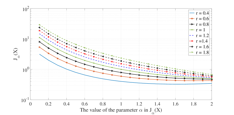
Figure 2: Evaluation of $J_{\alpha}(X)$ for $X\sim\mathcal{S}\left(r,(r)^{-\frac{1}{r}}\right)$ for different values of $\alpha$ and $r$

.

IV Generalized Information Theoretic Identities

In addition to their theoretical relevance, information inequalities have important implications in information theory. For example, by the means of the FII, one can prove the EPI which is useful for finding bounds on capacity regions and in proving strong versions of Central Limit Theorems (CLT)s. In what follows, we state and prove a list of information inequalities featuring $J_{\alpha}(\cdot)$. Namely, we list and prove a generalized FII, an upper bound on the differential entropy of sums having a stable component and a generalized IIE.

IV-A A Generalized Fisher Information Inequality

The Fisher information inequality is an important identity that relates the Fisher information of the sum of independent RVs to those of the individual variables. It was first proven by Stam [25] and then by Blachman [26]. Both authors deduced the EPI from the FII via de Bruijn’s identity. Stam relied on a data processing inequality of the Fisher information in the proof of the FII, a methodology that was later used by Zamir [40] in a more elaborate fashion. Finally, Rioul [35] derived a mutual information inequality, an identity that implies the EPI and by the means of de Bruijn’s identity implies the FII.

Data processing inequality for $J_{\alpha}$, $1<\alpha\leq 2$

The data processing inequality asserts that gains could not be achieved when processing information. In terms of mutual information, if the RVs $X\mbox{--}Y\mbox{--}Z$ form a Markov chain [30, p.34 Theorem 2.8.1],

$$I(Z;X)\leq I(Y;X),$$

with equality if $X\mbox{--}Z\mbox{--}Y$ is also a Markov chain. In [40], Zamir proved an equivalent inequality for the Fisher information in a variable $Y$ about a parameter $\theta$. We follow similar steps and extend the data processing inequality to $J_{\alpha}$; an inequality which we will use next to prove the GFII.

Definition 3.

Let $m>0$ and let $\bm{\theta}=\left[\theta_{1}\,\theta_{2}\,\cdots\,\theta_{m}\right]^{\text{t}}$ be a fixed vector of parameters. For $1<\alpha\leq 2$ define,

$$J_{\alpha}(\mathbf{Y}_{\bm{\theta}};\bm{\theta}) \;\hat{=}\;-\textsf{E}\left[{I^{\bm{\theta}}_{2-\alpha}\left[\bigtriangleup_{\bm{\theta}}\ln p_{\mathbf{Y}_{\bm{\theta}}}\right](\mathbf{Y}_{\bm{\theta}})}\right]$$ (22)

$$\&\qquad J_{\alpha}(\mathbf{Y}_{\bm{\theta}};\bm{\theta}|\mathbf{Z}) \;\hat{=}\;\quad\textsf{E}_{\mathbf{Z}}\left[{J_{\alpha}\left(\mathbf{Y}_{\bm{\theta}};\bm{\theta}|\mathbf{Z}=\mathbf{z}\right)}\right],$$

where for $f_{\bm{\theta}}(\cdot):\mathbb{R}^{d}\rightarrow\mathbb{R}$ that is parameterized by $\bm{\theta}\in\mathbb{R}^{m}$

$$I^{\bm{\theta}}_{2-\alpha}\left[f_{\bm{\theta}}\right]:\, \mathbb{R}^{d}\rightarrow\mathbb{R}$$

$$\mathbf{x}\,\,\,\rightarrow I^{\bm{\theta}}_{2-\alpha}\left[f_{\bm{\theta}}\right](\mathbf{x})=\frac{\Gamma\left(\frac{m}{2}-\frac{2-\alpha}{2}\right)}{\pi^{\frac{m}{2}}2^{2-\alpha}\Gamma\left(\frac{2-\alpha}{2}\right)}\int_{\mathbb{R}^{m}}\|\bm{\theta}-\bm{\eta}\|^{-m+2-\alpha}f_{\bm{\eta}}(\mathbf{x})\,d\bm{\eta},$$ (23)

and

$$\bigtriangleup_{\bm{\theta}}f_{\bm{\theta}}(\mathbf{x})=\sum_{i=1}^{m}\frac{\partial^{2}f_{\bm{\theta}}}{\partial\theta^{2}_{i}}(\mathbf{x}).$$

The operator $I_{2-\alpha}[\cdot]$ is the Riesz potential of order $(2-\alpha)$ presented in Appendix A. Note that the Riesz potential in equation (23) is that of function $f_{\bm{\theta}}(\cdot)$ when $\bm{\theta}$ is considered the variable instead of $\mathbf{x}$.

Theorem 5 (Translation Property for $d=m$).

If $d=m$ and $\mathbf{Y}_{\bm{\theta}}=\mathbf{Y}+\bm{\theta}$, then

$$J_{\alpha}(\mathbf{Y}_{\bm{\theta}};\bm{\theta})=J_{\alpha}(\mathbf{Y}).$$ (24)

Proof:

$$J_{\alpha}(\mathbf{Y}) =\int\ln p_{\mathbf{Y}}(\mathbf{y})\,\mathcal{F}_{\mathcal{I}}\bigl{[}\|\bm{\omega}\|^{\alpha}\phi_{\mathbf{Y}}(-\bm{\omega})\bigr{]}(\mathbf{y})\,d\mathbf{y}$$

$$=-\int\ln p_{\mathbf{Y}}(\mathbf{y})\,\bigtriangleup_{\mathbf{y}}\biggl{(}\mathcal{F}_{\mathcal{I}}\bigl{[}\|\bm{\omega}\|^{\alpha-2}\phi_{\mathbf{Y}}(-\bm{\omega})\bigr{]}(\mathbf{y})\biggr{)}\,d\mathbf{y}$$ (25)

$$=-\int\bigtriangleup_{\mathbf{y}}\left(\ln p_{\mathbf{Y}}(\mathbf{y})\right)\,I_{2-\alpha}[p_{\mathbf{Y}}](\mathbf{y})\,d\mathbf{y}$$ (26)

$$=-\int I_{2-\alpha}\left[\bigtriangleup_{\mathbf{y}}\left(\ln p_{\mathbf{Y}}\right)\right](\mathbf{y})\,p_{\mathbf{Y}}(\mathbf{y})\,d\mathbf{y}$$ (27)

$$=-\int I_{2-\alpha}\left[\sum_{j}\frac{d^{2}}{dy_{j}^{2}}\ln p_{\mathbf{Y}}\right](\mathbf{y})\,p_{\mathbf{Y}}(\mathbf{y})\,d\mathbf{y}$$ (28)

$$=-\int I^{\bm{\theta}}_{2-\alpha}\left[\sum_{j}\frac{d^{2}}{d\theta_{j}^{2}}\ln p_{\mathbf{Y}_{\bm{\theta}}}\right](\mathbf{y}+\bm{\theta})\,p_{\mathbf{Y}}(\mathbf{y})\,d\mathbf{y}$$ (29)

$$=-\int I^{\bm{\theta}}_{2-\alpha}\left[\bigtriangleup_{\bm{\theta}}\ln p_{\mathbf{Y}_{\bm{\theta}}}\right](\mathbf{y}+\bm{\theta})\,p_{\mathbf{Y}_{\bm{\theta}}}(\mathbf{y}+\bm{\theta})\,d\mathbf{y}$$

$$=J_{\alpha}(\mathbf{Y}_{\theta};\theta),$$

Equation (25) is due to basic properties of the Fourier transform since $I_{2-\alpha}(p_{\mathbf{Y}})(\mathbf{y})=\mathcal{F}_{\mathcal{I}}\left[\|\bm{\omega}\|^{\alpha-2}\phi_{\mathbf{Y}}(-\bm{\omega})\right](\mathbf{y})$ decays to $0$ at “$\infty$”. In order to write equation (26), we use Green’s first identity[41] in the following form: Let $\bigtriangledown$ denotes the gradient operator and $\times$ denotes the dot product. If $\Psi(\cdot)$ and $\Phi(\cdot)$ are real valued functions on $\mathbb{R}^{d}$, then

$$\int_{\mathbb{R}^{d}}\Psi(\mathbf{y})\bigtriangleup\Phi(\mathbf{y})\,d\mathbf{y}=-\int_{\mathbb{R}^{d}}\bigtriangledown\Psi(\mathbf{y})\times\bigtriangledown\Phi(\mathbf{y})\,d\mathbf{y}+\lim_{R\rightarrow+\infty}\int_{\|\mathbf{y}\|=R}\Psi(\mathbf{y})\bigtriangledown\Phi(\mathbf{y})\times\mathbf{n}\,dS(\mathbf{y}),$$

where $\mathbf{n}$ is the outward pointing unit normal vector of surface element $dS(\mathbf{y})$. Applying twice Green’s theorem justifies equation (26) as long as:

$$\lim_{R\rightarrow+\infty} \int_{\|\mathbf{y}\|=R}\ln p_{\mathbf{Y}}(\mathbf{y})\bigtriangledown I_{2-\alpha}(p_{\mathbf{Y}})(\mathbf{y})\times\mathbf{n}\,dS(\mathbf{y})=0$$

and

$$\lim_{R\rightarrow+\infty} \int_{\|\mathbf{y}\|=R}I_{2-\alpha}(p_{\mathbf{Y}})(\mathbf{y})\bigtriangledown\ln p_{\mathbf{Y}}(\mathbf{y})\times\mathbf{n}\,dS(\mathbf{y})=0.$$

As stated in Appendix A, equation (27) holds true whenever $\left|\bigtriangleup_{\mathbf{y}}\ln p_{\mathbf{Y}}(\mathbf{y})\right|\,I_{2-\alpha}(p_{\mathbf{Y}})(\mathbf{y})$ is integrable. It remains to justify equation (29) which we prove next,

$$I^{\bm{\theta}}_{2-\alpha}\left[\sum_{j}\frac{d^{2}}{d\theta_{j}^{2}}\ln p_{\mathbf{Y}_{\bm{\theta}}}\right](\mathbf{y}+\bm{\theta})$$

$$=\frac{\Gamma\left(\frac{d}{2}-\frac{2-\alpha}{2}\right)}{\pi^{\frac{d}{2}}2^{2-\alpha}\Gamma\left(\frac{2-\alpha}{2}\right)}\int_{\mathbb{R}^{d}}\|\bm{\theta}-\bm{\eta}\|^{-d+2-\alpha}\sum_{j}\frac{d^{2}}{d\eta_{j}^{2}}\ln p_{\mathbf{Y}_{\bm{\eta}}}(\mathbf{y}+\bm{\theta})\,d\bm{\eta}$$ (30)

$$=\frac{\Gamma\left(\frac{d}{2}-\frac{2-\alpha}{2}\right)}{\pi^{\frac{d}{2}}2^{2-\alpha}\Gamma\left(\frac{2-\alpha}{2}\right)}\int_{\mathbb{R}^{d}}\|\bm{\theta}-\bm{\eta}\|^{-d+2-\alpha}\sum_{j}\frac{d^{2}}{d\theta_{j}^{2}}\ln p_{\mathbf{Y}}(\mathbf{y}+\bm{\theta}-\bm{\eta})\,d\bm{\eta}$$ (31)

$$=\frac{\Gamma\left(\frac{d}{2}-\frac{2-\alpha}{2}\right)}{\pi^{\frac{d}{2}}2^{2-\alpha}\Gamma\left(\frac{2-\alpha}{2}\right)}\int_{\mathbb{R}^{d}}\|\bm{\theta}-\bm{\eta}\|^{-d+2-\alpha}\sum_{j}\frac{d^{2}}{dy_{j}^{2}}\ln p_{\mathbf{Y}}(\mathbf{y}+\bm{\theta}-\bm{\eta})\,d\bm{\eta}$$

$$=\frac{\Gamma\left(\frac{d}{2}-\frac{2-\alpha}{2}\right)}{\pi^{\frac{d}{2}}2^{2-\alpha}\Gamma\left(\frac{2-\alpha}{2}\right)}\int_{\mathbb{R}^{d}}\|\mathbf{y}-\mathbf{v}\|^{-d+2-\alpha}\sum_{j}\frac{d^{2}}{dy_{j}^{2}}\ln p_{\mathbf{Y}}(\mathbf{v})\,d\mathbf{v}$$ (32)

$$=I^{\bm{\theta}}_{2-\alpha}\left[\sum_{j}\frac{d^{2}}{dy_{j}^{2}}\ln p_{\mathbf{Y}}\right](\mathbf{y}).$$

Equation (30) is the definition of $I^{\bm{\theta}}_{2-\alpha}\left[\cdot\right]$ given in equation (23) and (31) is due to the fact that $\mathbf{Y}_{\bm{\eta}}=\mathbf{Y}+\bm{\eta}$. Equation (32) is obtained by the change of variable $\mathbf{v}=\mathbf{y}+\bm{\theta}-\bm{\eta}$ and the last equation is due to the definition of $I_{2-\alpha}\left[\cdot\right]$ (see Appendix A). ∎

Theorem 6 (Chain Rule and Data Processing Inequality for the $\alpha$-Fisher information ).

If $\bm{\theta}\text{--}\mathbf{Y}_{\bm{\theta}}\text{--}\mathbf{Z}_{\bm{\theta}}$, i.e., the conditional distribution of $\mathbf{Z}_{\bm{\theta}}$ given $\mathbf{Y}_{\bm{\theta}}$ is independent of $\bm{\theta}$, then

$$J_{\alpha}(\mathbf{Z}_{\bm{\theta}};\bm{\theta})\leq J_{\alpha}(\mathbf{Y}_{\bm{\theta}};\bm{\theta}),$$

whenever $J_{\alpha}(\mathbf{Y}_{\bm{\theta}};\bm{\theta}|\mathbf{Z}_{\bm{\theta}})\geq 0$.

We note that the condition $J_{\alpha}(\mathbf{Y}_{\bm{\theta}};\bm{\theta}|\mathbf{Z}_{\bm{\theta}})\geq 0$ is needed since there are no formal guarantees of non-negativeness according to Definition 3 as it is the case for $J_{\alpha}(\mathbf{Y})$. The non-negativity of $J_{\alpha}(\mathbf{Y}_{\bm{\theta}};\bm{\theta})$ is guaranteed, for example, whenever $\bm{\theta}$ is a translation parameter. Another case when non-negativity holds is found next in the proof of Theorem 7.

Proof:

Consider

$$J_{\alpha}(\mathbf{Y}_{\bm{\theta}},\mathbf{Z}_{\bm{\theta}};\bm{\theta})=-\textsf{E}_{\mathbf{Y},\mathbf{Z}}\left[{I_{2-\alpha}\left[\bigtriangleup_{\bm{\theta}}\left(\ln p_{\mathbf{Y}_{\bm{\theta}},\mathbf{Z}_{\bm{\theta}}}\right)\right](\mathbf{Y}_{\bm{\theta}},\mathbf{Z}_{\bm{\theta}})}\right].$$

We have

$$\ln p_{\mathbf{Y}_{\bm{\theta}},\mathbf{Z}_{\bm{\theta}}}(\mathbf{y},\mathbf{z};\bm{\theta})=\ln p_{\mathbf{Z}_{\bm{\theta}}}(\mathbf{z};\bm{\theta})+\ln p_{\mathbf{Y}_{\bm{\theta}}|\mathbf{Z}_{\bm{\theta}}}(\mathbf{y};\bm{\theta}|\mathbf{z}),$$

which yields

$$J_{\alpha}(\mathbf{Y}_{\theta},\mathbf{Z}_{\theta};\theta) = J_{\alpha}(\mathbf{Z}_{\theta};\theta)+J_{\alpha}(\mathbf{Y}_{\theta};\theta|\mathbf{Z}_{\theta})$$ (33)

$$\geq J_{\alpha}(\mathbf{Z}_{\theta};\theta).$$ (34)

Equation (33) is due to the linearity property of the Laplacian operator, the Riesz potential [42] and the expectation operator. Equation (34) is justified by the fact that $J_{\alpha}(\mathbf{Y}_{\theta};\theta|\mathbf{Z}_{\theta})\geq 0$ by assumption. Equality holds if and only if $J_{\alpha}(\mathbf{Y}_{\theta};\theta|\mathbf{Z}_{\theta})=0$ which is true if $\theta\text{--}\mathbf{Z}_{\theta}\text{--}\mathbf{Y}_{\theta}$ forms a Markov chain. On the other hand, since $\mathbf{Z}_{\theta}$ is conditionally independent of $\theta$ given $\mathbf{Y}_{\theta}$, $\ln p_{\mathbf{Z}_{\theta}|\mathbf{Y}_{\theta}}(\cdot|\mathbf{y})$ is independent of $\theta$ and

$$J_{\alpha}(\mathbf{Y}_{\theta},\mathbf{Z}_{\theta};\theta)=J_{\alpha}(\mathbf{Y}_{\theta};\theta),$$

which along with equation (34) gives the required result. ∎

Additivity property of $J_{\alpha}(\mathbf{Y})$ for vectors $\mathbf{Y}$ having independent components

Before proceeding to state and prove the GFII, we prove the additivity of $J_{\alpha}(\mathbf{Y})$ when $\mathbf{Y}$ has independent components, as mentioned in property (7). Starting from equation (28),

$$J_{\alpha}(\mathbf{Y}) = -\int p_{\mathbf{Y}}(\mathbf{y})\,I_{2-\alpha}\left[\sum_{j}\frac{d^{2}}{dy_{j}^{2}}\ln p_{\mathbf{Y}}\right](\mathbf{y})\,d\mathbf{y}$$ (35)

$$= -\int p_{\mathbf{Y}}(\mathbf{y})\,I_{2-\alpha}\left[\sum_{j}\frac{d^{2}}{dy_{j}^{2}}\ln p_{Y_{j}}\right](\mathbf{y})\,d\mathbf{y}$$

$$= -\sum_{j}\int p_{\mathbf{Y}}(\mathbf{y})\,I_{2-\alpha}\left[\frac{d^{2}}{dy_{j}^{2}}\ln p_{Y_{j}}\right](y_{j})\,d\mathbf{y}$$ (36)

$$= -\sum_{j}\int p_{Y_{j}}(y_{j})\,I_{2-\alpha}\left[\frac{d^{2}}{dy_{j}^{2}}\ln p_{Y_{j}}\right](y_{j})\,dy_{j}$$ (37)

$$= -\sum_{j}\int\frac{d^{2}}{dy_{j}^{2}}I_{2-\alpha}\left[p_{\mathbf{Y}}(\mathbf{y})\right]\,\ln p_{Y_{j}}(y_{j})\,dy_{j}$$

$$= \sum_{j}J_{\alpha}(Y_{j}),$$

where equations (35) and (37) are due to the independence of the $Y_{j}$’s. Equation (36) is justified by the linearity of the Riesz potential and equation (IV-A) holds true whenever $\left\{\ln p_{Y_{j}}\frac{d}{dy_{j}}I_{2-\alpha}[p_{Y_{j}}](y_{j})\right\}_{j}$ go to $0$ at “$\infty$” and the regularity condition (17) is satisfied by the $\left\{Y_{j}\right\}$’s.

Generalized Fisher Information Inequality

Theorem 7 (Generalized Fisher Information Inequality (GFII)).

Let $1<\alpha\leq 2$ and let $\mathbf{Y}_{1}$ and $\mathbf{Y}_{2}$ be two independent $d$-dimensional random vectors, then

$$J^{\frac{1}{1-\alpha}}_{\alpha}(\mathbf{Y}_{1}+\mathbf{Y}_{2})\geq J^{\frac{1}{1-\alpha}}_{\alpha}(\mathbf{Y}_{1})+J^{\frac{1}{1-\alpha}}_{\alpha}(\mathbf{Y}_{2}).$$ (39)

We note that whenever $\alpha=2$, equation (39) boils down to the well-known “classical” FII.

Proof:

For the matter of the proof, we make use of the data processing inequality established in Theorem 6. Let $\omega_{1}$ and $\omega_{2}\in\mathbb{R}^{+*}$ be two positive numbers such that $\omega_{1}+\omega_{2}=1$. Also let $\epsilon>0$ and ${\bf N}$ be an independent random vector distributed according to $\bm{\mathcal{S}}(\alpha,1)$. For any $\bm{\theta}\in\mathbb{R}^{d}$ we have

$$\bm{\theta}-\left(\frac{\mathbf{Y}_{1}}{\omega_{1}}+\bm{\theta},\frac{\mathbf{Y}_{2}}{\omega_{2}}+\bm{\theta}\right)-(\mathbf{Y}_{1}+\mathbf{Y}_{2}+\bm{\theta}+\sqrt[\alpha]{\epsilon}{\bf N})$$

forms a Markov chain. Define $\mathbf{Y}_{\bm{\theta},1}=\frac{\mathbf{Y}_{1}}{\omega_{1}}+\bm{\theta}$, $\mathbf{Y}_{\bm{\theta},2}=\frac{\mathbf{Y}_{2}}{\omega_{2}}+\bm{\theta}$ and $\mathbf{Z}_{\bm{\theta}}=\omega_{1}\mathbf{Y}_{\bm{\theta},1}+\omega_{2}\mathbf{Y}_{\bm{\theta},2}+\sqrt[\alpha]{\epsilon}\mathbf{N}$, then

$$J_{\alpha}\left(\left(\mathbf{Y}_{\bm{\theta},1},\mathbf{Y}_{\bm{\theta},2}\right);\bm{\theta}\Big{|}\mathbf{Z}_{\bm{\theta}}\right)\;\hat{=}\;\textsf{E}_{\mathbf{Z}_{\bm{\theta}}}\left[{J_{\alpha}\left(\left(\mathbf{Y}_{\bm{\theta},1},\mathbf{Y}_{\bm{\theta},2}\right);\bm{\theta}|\mathbf{Z}_{\bm{\theta}}\right)}\right]\geq 0.$$

Indeed, let $p_{\left(\mathbf{Y}_{\bm{\theta},1},\mathbf{Y}_{\bm{\theta},2}\right)|\mathbf{Z}_{\bm{\theta}}}(\cdot,\cdot|\mathbf{z})$ be the PDF of $\left(\mathbf{Y}_{\bm{\theta},1},\mathbf{Y}_{\bm{\theta},2}\right)$ given $\mathbf{Z}_{\bm{\theta}}=\mathbf{z}$. Then,

$$p_{\left(\mathbf{Y}_{\bm{\theta},1},\mathbf{Y}_{\bm{\theta},2}\right)|\mathbf{Z}_{\bm{\theta}}}(\mathbf{y}_{1},\mathbf{y}_{2}|\mathbf{z}) = p_{\mathbf{Y}_{\bm{\theta},1}|\mathbf{Z}_{\bm{\theta}}}(\mathbf{y}_{1}|\mathbf{z})\,p_{\mathbf{Y}_{\bm{\theta},2}|\mathbf{Y}_{\bm{\theta},1},\mathbf{Z}_{\bm{\theta}}}(\mathbf{y}_{2}|\mathbf{y}_{1},\mathbf{z})$$

$$= p_{\frac{\mathbf{Y}_{1}}{\omega_{1}}|\mathbf{Z}_{\bm{\theta}}}(\mathbf{y}_{1}-\bm{\theta}|\mathbf{z})\,p_{\sqrt[\alpha]{\epsilon}{\bf N}|\mathbf{Y}_{\bm{\theta},1},\mathbf{Z}_{\bm{\theta}}}(\mathbf{z}-\omega_{1}\mathbf{y}_{1}-\omega_{2}\mathbf{y}_{2}|\mathbf{y}_{1},\mathbf{z}).$$

One can now write:

$$J_{\alpha}\left(\left(\mathbf{Y}_{\bm{\theta},1},\mathbf{Y}_{\bm{\theta},2}\right);\bm{\theta}\Big{|}\mathbf{Z}_{\bm{\theta}}=\mathbf{z}\right) = J_{\alpha}\left(\mathbf{Y}_{\bm{\theta},1};\bm{\theta}\Big{|}\mathbf{Z}_{\bm{\theta}}=\mathbf{z}\right)+J_{\alpha}\left(\mathbf{Y}_{\bm{\theta},2};\bm{\theta}\Big{|}\left(\mathbf{Y}_{\bm{\theta},1},\mathbf{Z}_{\bm{\theta}}=\mathbf{z}\right)\right)$$ (40)

$$= J_{\alpha}\left(\frac{\mathbf{Y}_{1}}{\omega_{1}}\Big{|}\mathbf{Z}_{\bm{\theta}}=\mathbf{z}\right)+J_{\alpha}\left(\mathbf{Y}_{\bm{\theta},2};\bm{\theta}\Big{|}\left(\mathbf{Y}_{\bm{\theta},1},\mathbf{Z}_{\bm{\theta}}=\mathbf{z}\right)\right)$$

$$= J_{\alpha}\left(\frac{\mathbf{Y}_{1}}{\omega_{1}}\Big{|}\mathbf{Z}_{\bm{\theta}}=\mathbf{z}\right),$$

where we used Theorem 5 and the fact that

$$J_{\alpha}\left(\mathbf{Y}_{\bm{\theta},2};\bm{\theta}\Big{|}\left(\mathbf{Y}_{\bm{\theta},1},\mathbf{Z}_{\bm{\theta}}=\mathbf{z}\right)\right)=\textsf{E}_{\mathbf{Y}_{\bm{\theta},1}}\left[{J_{\alpha}\left(\mathbf{Y}_{\bm{\theta},2};\bm{\theta}\Big{|}\left(\mathbf{Y}_{\bm{\theta},1},\mathbf{Z}_{\bm{\theta}}=\mathbf{z}\right)\right)}\right]=0,$$

since $J_{\alpha}\left(\mathbf{Y}_{\bm{\theta},2};\bm{\theta}\Big{|}\left(\mathbf{Y}_{\bm{\theta},1}=\mathbf{y}_{1},\mathbf{Z}_{\bm{\theta}}=\mathbf{z}\right)\right)=0$ for every $\mathbf{y}_{1}$ because $p_{\mathbf{Y}_{\bm{\theta},2}|\left(\mathbf{Y}_{\bm{\theta},1},\mathbf{Z}_{\bm{\theta}}\right)}(\cdot)$ is independent of $\bm{\theta}$. Equation (40) is non-negative by property (1) and therefore by Theorem 6,

$$J_{\alpha}\left(\mathbf{Z}_{\bm{\theta}};\bm{\theta}\right) \leq J_{\alpha}\left(\left(\mathbf{Y}_{\bm{\theta},1},\mathbf{Y}_{\bm{\theta},2}\right);\bm{\theta}\right).$$ (41)

Since $\mathbf{Y}_{\bm{\theta},1}$ and $\mathbf{Y}_{\bm{\theta},2}$ are statistically independent and using the definition of $J_{\alpha}(\cdot;\bm{\theta})$ in (22), the RHS of equation (41) boils down to:

$$J_{\alpha}\left(\left(\mathbf{Y}_{\bm{\theta},1},\mathbf{Y}_{\bm{\theta},2}\right);\bm{\theta}\right)=J_{\alpha}\left(\mathbf{Y}_{\bm{\theta},1};\bm{\theta}\right)+J_{\alpha}\left(\mathbf{Y}_{\bm{\theta},2};\bm{\theta}\right),$$

which implies by means of the translation invariance property (2) in (24) that equation (41) is equivalent to:

$$J_{\alpha}\left(\mathbf{Y}_{1}+\mathbf{Y}_{2}+\sqrt[\alpha]{\epsilon}\mathbf{N}\right).\leq J_{\alpha}\left(\frac{\mathbf{Y}_{1}}{\omega_{1}}\right)+J_{\alpha}\left(\frac{\mathbf{Y}_{2}}{\omega_{2}}\right),$$

Under the regularity condition (17), taking the limit as $\epsilon\rightarrow 0$ yields

$$J_{\alpha}\left(\mathbf{Y}_{1}+\mathbf{Y}_{2}\right) \leq J_{\alpha}\left(\frac{\mathbf{Y}_{1}}{\omega_{1}}\right)+J_{\alpha}\left(\frac{\mathbf{Y}_{2}}{\omega_{2}}\right)$$ (42)

$$\leq \omega_{1}^{\alpha}J_{\alpha}(\mathbf{Y}_{1})+\omega_{2}^{\alpha}J_{\alpha}(\mathbf{Y}_{2}),$$

by property (5) of $J_{\alpha}(\cdot)$. Equation (42) holds true for any $\omega_{1}$ and $\omega_{2}$ satisfying the conditions of the theorem, the tightest choice $\omega_{1}^{*}$ and $\omega_{2}^{*}$ being,

$$\omega_{1}^{*} =\arg\min_{0\leq\omega_{1}\leq 1}\,\{\omega_{1}^{\alpha}J_{\alpha}(\mathbf{Y}_{1})+(1-\omega_{1})^{\alpha}J_{\alpha}(\mathbf{Y}_{2})\}$$

$$=\frac{J^{\frac{1}{\alpha-1}}_{\alpha}(\mathbf{Y}_{2})}{J^{\frac{1}{\alpha-1}}_{\alpha}(\mathbf{Y}_{1})+J^{\frac{1}{\alpha-1}}_{\alpha}(\mathbf{Y}_{2})}$$

$$\omega_{2}^{*} =1-\omega_{1}^{*}=\frac{J^{\frac{1}{\alpha-1}}_{\alpha}(\mathbf{Y}_{1})}{J^{\frac{1}{\alpha-1}}_{\alpha}(\mathbf{Y}_{1})+J^{\frac{1}{\alpha-1}}_{\alpha}(\mathbf{Y}_{2})},$$

for which (42) becomes

$$J_{\alpha}\left(\mathbf{Y}_{1}+\mathbf{Y}_{2}\right)\leq\frac{J_{\alpha}(\mathbf{Y}_{1})J_{\alpha}(\mathbf{Y}_{2})}{\left[J^{\frac{1}{\alpha-1}}_{\alpha}(\mathbf{Y}_{1})+J^{\frac{1}{\alpha-1}}_{\alpha}(\mathbf{Y}_{2})\right]^{\alpha-1}},$$

which completes the proof of the theorem. ∎

IV-B Upper Bounds on the Differential Entropy of Sums Having a Stable Component

An important category of information inequalities consists of finding upper bounds on the entropy of independent sums. Starting with fundamental inequalities such that the upper bound on the discrete entropy of independent sums [30] and the upper bound on the differential entropy of the sum of independent finite-variance RVs [23], several identities involving discrete and differential entropy of sums were subsequently shown in [43, 44, 45, 46, 47, 48, 49]. Recently in [36], an upper bound on the differential entropy of the sum $X+N$ of two independent RVs was found where $N$ is a finite-variance infinitely divisible variable having a Gaussian component. We extend in this section the known upper bound results to cases where $\mathbf{N}$ is SS stable vector using the GFII and the generalized de Bruijn’s identity.

Theorem 8 (Upper bound on the Entropy of Sums having a Stable Component).

Let $\mathbf{Z}\sim\bm{\mathcal{S}}\left(\alpha,\gamma\right)$, $1<\alpha\leq 2$, and let $\mathbf{X}$ be a $d$-dimensional vector that is independent of $\mathbf{Z}$ such that $h(\mathbf{X})$ and $J_{\alpha}(\mathbf{X})$ are finite. Then

$$h(\mathbf{X}+\mathbf{Z})-h(\mathbf{X})\leq\gamma^{\alpha}J_{\alpha}(\mathbf{X})\,_{2}F_{1}\left(\alpha-1,\alpha-1;\alpha;-\left(\frac{\alpha\gamma^{\alpha}}{d}J_{\alpha}(\mathbf{X})\right)^{\frac{1}{\alpha-1}}\right),$$

where ${}_{2}F_{1}(a,b;c;z)$ is the analytic continuation of the Gauss hypergeometric function on the complex plane with a cut along the real axis from 1 to +$\infty$.

For more details on hypergeometric functions, the reader may refer to Appendix A. Theorem 8 provides an upper bound on the entropy of the sum of two variables when one of them is stable. As a special case, when $\alpha=2$, it recovers the upper bound for Gaussian noise setups [36].

Proof:

Using the extended de Bruijn’s identity (20), we write:

$$h(\mathbf{X}+\mathbf{Z})-h(\mathbf{X}) =\int^{1}_{0}\gamma^{\alpha}J_{\alpha}(\mathbf{X}+\sqrt[\alpha]{\eta}\mathbf{Z})\,d\eta$$

$$\leq\gamma^{\alpha}\int^{1}_{0}\frac{J_{\alpha}(\mathbf{X})J_{\alpha}(\sqrt[\alpha]{\eta}\mathbf{Z})}{\left(J^{\frac{1}{\alpha-1}}_{\alpha}(\mathbf{X})+J^{\frac{1}{\alpha-1}}_{\alpha}(\sqrt[\alpha]{\eta}\mathbf{Z})\right)^{\alpha-1}}\,d\eta$$ (43)

$$=\gamma^{\alpha}\int^{1}_{0}\frac{J_{\alpha}(\mathbf{X})\frac{d}{\alpha\gamma^{\alpha}\eta}}{\left(J^{\frac{1}{\alpha-1}}_{\alpha}(\mathbf{X})+(\frac{d}{\alpha\gamma^{\alpha}\eta})^{\frac{1}{\alpha-1}}\right)^{\alpha-1}}\,d\eta$$ (44)

$$=(\alpha-1)\gamma^{\alpha}J_{\alpha}(\mathbf{X})\int_{0}^{1}\frac{u^{\alpha-2}}{\left((\frac{\alpha\gamma^{\alpha}}{d}J_{\alpha}(\mathbf{X}))^{\frac{1}{\alpha-1}}u+1\right)^{\alpha-1}}du$$

$$=\gamma^{\alpha}J_{\alpha}(\mathbf{X})\,_{2}F_{1}\left(\alpha-1,\alpha-1;\alpha;-\left(\frac{\alpha\gamma^{\alpha}}{d}J_{\alpha}(\mathbf{X})\right)^{\frac{1}{\alpha-1}}\right),$$ (45)

where we use the GFII in order to write equation (43) and properties (4) and (5) of $J_{\alpha}(\cdot)$ to validate equation (44). ∎

Interestingly, Theorem 8 gives an analytical bound on the change in the transmission rates of the linear stable channel function of an input scaling operation: let $a\neq 0$, then

$$h(a\mathbf{X}+\mathbf{Z}) \leq h(a\mathbf{X})+\gamma^{\alpha}J_{\alpha}(a\mathbf{X})\,_{2}F_{1}\left(\alpha-1,\alpha-1;\alpha;-\left(\frac{\alpha\gamma^{\alpha}}{d}J_{\alpha}(a\mathbf{X})\right)^{\frac{1}{\alpha-1}}\right),$$

$$=h(\mathbf{X})+d\ln|a|+\left(\frac{\gamma}{|a|}\right)^{\alpha}J_{\alpha}(\mathbf{X})\,_{2}F_{1}\left(\alpha-1,\alpha-1;\alpha;-\left(\frac{\alpha}{d}\left(\frac{\gamma}{|a|}\right)^{\alpha}J_{\alpha}(\mathbf{X})\right)^{\frac{1}{\alpha-1}}\right),$$

where we used the fact that $h(a\mathbf{X})=h(\mathbf{X})+d\ln|a|$ and $J_{\alpha}(a\mathbf{X})=\frac{1}{|a|^{\alpha}}J_{\alpha}(\mathbf{X})$. Subtracting $h(\mathbf{Z})$ from both sides of the equation gives

$$I(a\mathbf{X}+\mathbf{Z};\mathbf{X})-I(\mathbf{X}+\mathbf{Z};\mathbf{X})\leq\ln|a|+\left(\frac{\gamma}{|a|}\right)^{\alpha}J_{\alpha}(\mathbf{X})\,_{2}F_{1}\left(\alpha-1,\alpha-1;\alpha;-\left(\frac{\alpha}{d}\left(\frac{\gamma}{a}\right)^{\alpha}J_{\alpha}(\mathbf{X})\right)^{\frac{1}{\alpha-1}}\right).$$

Since ${}_{2}F_{1}\left(\alpha-1,\alpha-1;\alpha;0\right)=1$,

$$\lim_{|a|\rightarrow+\infty}\left(\frac{\gamma}{a}\right)^{\alpha}J_{\alpha}(\mathbf{X})\,_{2}F_{1}\left(\alpha-1,\alpha-1;\alpha;-\left(\frac{\alpha}{d}\left(\frac{\gamma}{a}\right)^{\alpha}J_{\alpha}(\mathbf{X})\right)^{\frac{1}{\alpha-1}}\right)=0,$$

and for large values of $|a|$ the variation in the transmissions rates is bounded by a logarithmically growing function of $|a|$. This is a known behavior of the optimal transmission rates that are achieved by Gaussian inputs in a Gaussian setting.

On a final note, making use of the identity:

$$\ln(1+t)=t_{2}F_{1}(1,1;2;-t),$$

equation (45) when evaluated for $\mathbf{Z}\sim\bm{\mathcal{N}}(0;\sigma^{2}\textsf{I})$ and $\alpha=2$ boils down to the following:

Corollary 1 (Upper bound on the Entropy of Sums having a Gaussian Component).

[36]

Let $\mathbf{Z}\sim\bm{\mathcal{N}}(0,\sigma^{2}\textsf{I})$ and $\mathbf{X}$ be a $d$-dimensional vector that is independent of $\mathbf{Z}$ such that $h(\mathbf{X})$ and $J(\mathbf{X})$ are finite. The differential entropy of $\mathbf{X}+\mathbf{Z}$ is upper bounded by:

$$h(\mathbf{X}+\mathbf{Z})\leq h(\mathbf{X})+\frac{d}{2}\ln\left(1+\frac{\sigma^{2}}{d}J(\mathbf{X})\right),$$ (46)

and equality holds if and only if both $X$ and $Z$ are Gaussian distributed.

As shown in [36, Section 4], we note that (46) implies a reverse EPI when one of the vectors is Gaussian distributed, which is equivalent to the concavity of the entropy power proved by Costa [50]. This was noted by Courtade [51] who provided a generalization of the reverse EPI in [52, Theorem 5].

IV-C A Generalized Isoperimetric Inequality for Entropies

Let ${\bf\tilde{Z}_{\alpha}\!}\sim\bm{\mathcal{S}}\left(\alpha,(\frac{1}{\alpha})^{\frac{1}{\alpha}}\right)$ and define $N_{\alpha}(\mathbf{X})$, $0<\alpha\leq 2$, the entropy power of order $\alpha$ as

$$N_{\alpha}(\mathbf{X})=\frac{1}{e^{\frac{\alpha}{d}h({\bf\tilde{Z}_{\alpha}\!})}}e^{\frac{\alpha}{d}h(\mathbf{X})}.$$ (47)

Theorem 9 (Generalized Isoperimetric Inequality for Entropies (GIIE)).

Let $\mathbf{X}$ be a d-dimensional random vector such that both $h(\mathbf{X})$ and $J_{\alpha}(\mathbf{X})$ exist, for some $1<\alpha\leq 2$. Then

$$\frac{1}{d}\,N_{\alpha}(\mathbf{X})J_{\alpha}(\mathbf{X})\geq\,\kappa_{\alpha}\;\hat{=}\;e^{(\alpha-1)\left(\psi(\alpha)+\gamma_{\text{e}}\right)-1},$$ (48)

where $\gamma_{\text{e}}$ is the Euler-Mascheroni constant and $\psi(\cdot)$ is the digamma function.

Since $\psi(2)=-\gamma_{\text{e}}+1$, we note right away that the evaluation (48) for $\alpha=2$ yields the well known IIE [27, Theorem 16]:

$$\frac{1}{d}\,N(\mathbf{X})J(\mathbf{X})\geq 1,$$

with equality when $\mathbf{X}$ is Gaussian distributed. For general values of $1<\alpha\leq 2$, whether equality in equation (48) is achievable or not and under which conditions are still not answered.

Proof:

Let $t=\left(\frac{\alpha\gamma^{\alpha}}{d}J_{\alpha}(\mathbf{X})\right)^{\frac{1}{\alpha-1}}$ and $\mathbf{Z}\sim\bm{\mathcal{S}}\left(\alpha,\gamma\right)$. By Theorem 8,

$$\frac{\alpha}{d}(h(\mathbf{X}+\mathbf{Z})-h(\mathbf{X})) =t^{\alpha-1}\,_{2}F_{1}\left(\alpha-1,\alpha-1;\alpha;-t\right)$$

$$=\left(\frac{t}{1+t}\right)^{\alpha-1}\,_{2}F_{1}\left(\alpha-1,1;\alpha;\frac{t}{1+t}\right),$$ (49)

where we used the fact that $t>0$ and a transformation property of the Gauss hypergeometric function as presented in Appendix A. Using the series representation of the Gauss hypergeometric function on the open unit disk, one can write:

$${}_{2}F_{1}\left(\alpha-1,1;\alpha;\frac{t}{1+t}\right) = \sum^{+\infty}_{n=0}\frac{(\alpha-1)_{n}(1)_{n}}{(\alpha)_{n}}\left(\frac{t}{1+t}\right)^{n}$$

$$= \sum^{+\infty}_{n=0}\frac{\alpha-1}{n+\alpha-1}\left(\frac{t}{1+t}\right)^{n},$$

where $(A)_{n}=\frac{\Gamma(A+n)}{\Gamma(A)}$. Equation (49) can hence be written as,

$$\frac{\alpha}{d}(h(\mathbf{X}+\mathbf{Z})-h(\mathbf{X}))=(\alpha-1)\left(\frac{t}{1+t}\right)^{\alpha-1}\sum^{+\infty}_{n=0}\frac{1}{n+\alpha-1}\left(\frac{t}{1+t}\right)^{n}.$$ (50)

The LHS of equation (50) is lower bounded by:

$$\frac{\alpha}{d}(h(\mathbf{X}+\mathbf{Z})-h(\mathbf{X}))\geq\frac{\alpha}{d}(h(\mathbf{Z})-h(\mathbf{X}))=\ln\frac{t^{\alpha-1}}{\frac{N_{\alpha}(\mathbf{X})J_{\alpha}(\mathbf{X})}{d}},$$

where we used equation (47), the fact that $t=\left(\frac{\alpha\gamma^{\alpha}}{d}J_{\alpha}(\mathbf{X})\right)^{\frac{1}{\alpha-1}}$ and that $h(\mathbf{Z})=d\ln\left(\gamma\alpha^{\frac{1}{\alpha}}\right)+h({\bf\tilde{Z}_{\alpha}\!})$ in order to write the equality. As for the RHS of (50),

$$(\alpha-1)\left(\frac{t}{1+t}\right)^{\alpha-1}\sum^{+\infty}_{n=0}\frac{1}{n+\alpha-1}\left(\frac{t}{1+t}\right)^{n}$$

$$=\,\, (\alpha-1)\left(\frac{t}{1+t}\right)^{\alpha-1}\left[\frac{1}{\alpha-1}-\ln\left(1-\frac{t}{1+t}\right)-(\alpha-1)\sum^{+\infty}_{n=1}\frac{1}{n(\alpha+n-1)}\left(\frac{t}{1+t}\right)^{n}\right]$$

$$=\,\, \left(\frac{t}{1+t}\right)^{\alpha-1}+(\alpha-1)\left(\frac{t}{1+t}\right)^{\alpha-1}\ln(1+t)-(\alpha-1)^{2}\sum^{+\infty}_{n=1}\frac{1}{n(\alpha+n-1)}\left(\frac{t}{1+t}\right)^{n+\alpha-1}.$$

Therefore (50) implies for any $t>0$:

$$\ln\left[\frac{N_{\alpha}(\mathbf{X})J_{\alpha}(\mathbf{X})}{d}\right]-(\alpha-1)\ln t\geq-\left(\frac{t}{1+t}\right)^{\alpha-1}-(\alpha-1)\left(\frac{t}{1+t}\right)^{\alpha-1}\ln(1+t)\\ +(\alpha-1)^{2}\sum^{+\infty}_{n=1}\frac{1}{n(\alpha+n-1)}\left(\frac{t}{1+t}\right)^{n+\alpha-1},$$

which by letting the scale $\gamma\rightarrow+\infty$ –and therefore $t\rightarrow+\infty$, gives the required result

$$\ln N_{\alpha}(\mathbf{X})J_{\alpha}(\mathbf{X}) \geq(\alpha-1)^{2}\sum^{+\infty}_{n=1}\frac{1}{n(\alpha+n-1)}-1$$ (51)

$$=(\alpha-1)\left(\psi(\alpha)+\gamma_{\text{e}}\right)-1.$$

The fact that the series $\sum_{n=1}^{+\infty}\frac{1}{n(\alpha+n-1)}\left(\frac{t}{1+t}\right)^{n+\alpha-1}$ is absolutely convergent permits the interchange in the order of the limits and justifies equation (51). ∎

We plot in Figure 3 the evaluation of the LHS of equation (48) at the values of $\alpha=[1.2,1.4,1.6,1.8]$ for alpha-stable RVs $\mathcal{S}\left(r,(r)^{-\frac{1}{r}}\right)$ for the values of $r=[0.4,0.6,0.8,1,1.2,1.4,1.6,1.8]$. The horizontal lines represent the RHS of equation (48) for the considered values of $\alpha$. Note that stable variables do not achieve the lower bound of the GIIE (48) except when $\alpha=2$ where Gaussian variables achieve the lower bound. The tightness in (48) is explored in Figure 4 where we evaluate the product $N_{1.8}(X)J_{1.8}(X)$ whenever $X=X_{1}+X_{2}$ where $X_{1}\sim\mathcal{S}\left(r,(r)^{-\frac{1}{r}}\right)$ for $r=1.8$ and $X_{2}\sim\mathcal{N}(0,\sigma^{2})$ for different value of $\sigma$. The minimum is achieved for $\sigma=4$ and not when $X$ is alpha-stable (i.e., when $\sigma=0$). Note that the computed minimum in Figure 4 is by no means a global minimum.

Whether there exist RVs that achieve the minimum of $N_{\alpha}(X)J_{\alpha}(X)$ and whether the lower bound $\kappa_{\alpha}$ is tight or not are still to be determined.

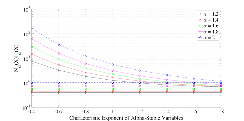
Figure 3: Evaluation of $N_{\alpha}(X)J_{\alpha}(X)$ and comparing it to $\kappa_{\alpha}$ for $X\sim\mathcal{S}\left(r,(r)^{-\frac{1}{r}}\right)$ for different values of $\alpha$ and $r$.

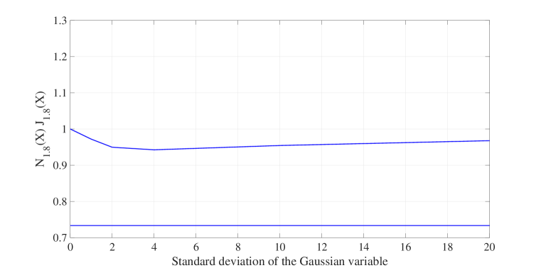
Figure 4: Comparison of $N_{1.8}(X)J_{1.8}(X)$ to $\kappa_{1.8}=0.7333$ for $X=X_{1}+X_{2}$ where $X_{1}\sim\mathcal{S}\left(r,(r)^{-\frac{1}{r}}\right)$, $r=1.8$ and $X_{2}\sim\mathcal{N}(0,\sigma^{2})$ for different values of $\sigma$.

Figure 5 shows the relative tightness of the lower bound $\kappa_{\alpha}$ when the LHS of equation (48) is evaluated at alpha-stable variables with characteristic exponents $r$ ranging from $0.4$ to $1.8$. If we consider for example on the $x$-axis the value of $r=0.8$ which corresponds to the alpha-stable variable $X\sim\mathcal{S}\left(r,(r)^{-\frac{1}{r}}\right)$, the figure shows that as $\alpha$ decreases, $N_{\alpha}(X)J_{\alpha}(X)$ gets closer to $\kappa_{\alpha}$ in a relative manner.

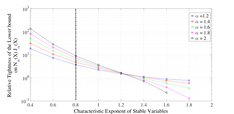
Figure 5: Relative tightness of $\kappa_{\alpha}$ for alpha-stable variables.

V Parameter Estimation in Impulsive Noise Environments: A Generalized Cramer-Rao Bound

Consider now the problem of estimating a non-random vector of parameters $\bm{\theta}\in\mathbb{R}^{d}$ based on a noisy observation $\mathbf{X}$ where the additive noise $\mathbf{N}$ is of impulsive nature. Needless to say that in this case the MSE criterion and the MMSE estimator are not adequate. More explicitly, let

$$\mathbf{X}=\bm{\theta}+\mathbf{N},$$

where $\mathbf{N}$ is a noise variable having both $h(\mathbf{N})$ and $J_{\alpha}(\mathbf{N})$ (for some $1<\alpha\leq 2$) exist and finite. Let $\hat{\bm{\theta}}(\mathbf{X})$ be an estimator of $\bm{\theta}$ based on the observation of the random vector $\mathbf{X}$. A good indicator of the quality of the estimator $\hat{\bm{\theta}}(\mathbf{X})$ is the power of the “error” $\left(\hat{\bm{\theta}}(\mathbf{X})-\bm{\theta}\right)$. We find next a lower bound on such metric which generalizes the previously known Cramer-Rao bound.

Theorem 10 (Generalized Cramer-Rao Bound).

Let $\hat{\bm{\theta}}(\mathbf{X})$ be an estimator of the parameter $\bm{\theta}$ based on the observation $\mathbf{X}=\bm{\theta}+\mathbf{N}$. Then the $\alpha$-power of the error is lower bounded by

$$\text{P}_{\!\alpha\!}\left({\text{e}}\right)=\text{P}_{\!\alpha\!}\left({\hat{\bm{\theta}}(\mathbf{X})-\bm{\theta}}\right)\geq\left(\frac{d\kappa_{\alpha}}{J_{\alpha}(\mathbf{N})}\right)^{\frac{1}{\alpha}}.$$ (52)

Note that whenever $\alpha=2$ the result of Theorem 10 is the classical Cramer-Rao bound when $\mathbf{N}$ has IID components. It gives a looser version for general $\mathbf{N}$:

$$\frac{\textsf{E}\left[{\left\|\hat{\bm{\theta}}(\mathbf{X})-\bm{\theta}\right\|^{2}}\right]}{d}\geq\frac{d}{J(\mathbf{N})}.$$ (53)

Proof:

Using Theorem 1, among all random vectors that have an $\alpha$-power equal to $\text{P}_{\!\alpha\!}\left({\text{e}}\right)$, the entropy maximizing variable is distributed according to $\bm{\mathcal{S}}\left(\alpha,\left(\frac{1}{\alpha}\right)^{\frac{1}{\alpha}}\text{P}_{\!\alpha\!}\left({\text{e}}\right)\right)$ and

$$h\left(\hat{\bm{\theta}}(\mathbf{X})-\bm{\theta}\right)\leq h({\bf\tilde{Z}_{\alpha}\!})+d\ln\text{P}_{\!\alpha\!}\left({\text{e}}\right),$$

which implies that

$$N_{\alpha}\left(\hat{\bm{\theta}}(\mathbf{X})-\bm{\theta}\right)\leq\text{P}_{\!\alpha\!}\left({\text{e}}\right)^{\alpha}.$$ (54)

On the other hand,

$$J_{\alpha}\left(\hat{\bm{\theta}}(\mathbf{X})-\bm{\theta}\right)=J_{\alpha}\left(\hat{\bm{\theta}}(\mathbf{X})\right)=J_{\alpha}\left(\hat{\bm{\theta}}(\mathbf{X});\bm{\theta}\right)\leq J_{\alpha}(\mathbf{X};\bm{\theta})=J_{\alpha}(\mathbf{N}),$$ (55)

where the second and the last equalities are due to Theorem 5 and the inequality is due to the data processing inequality for $J_{\alpha}(\cdot)$ proven in Theorem 6. Applying the GIIE (48) to $\hat{\bm{\theta}}(\mathbf{X})-\bm{\theta}$, we obtain:

$$\frac{N_{\alpha}\left(\hat{\bm{\theta}}(\mathbf{X})-\bm{\theta}\right)J_{\alpha}\left(\hat{\bm{\theta}}(\mathbf{X})-\bm{\theta}\right)}{d}\geq\kappa_{\alpha},$$

which along with equations (54) and (55) gives,

$$\frac{J_{\alpha}(\mathbf{N})\,\text{P}_{\!\alpha\!}\left({\text{e}}\right)^{\alpha}}{d}\geq\kappa_{\alpha}.$$

∎

Whenever the noise is a SS vector $\mathbf{N}\sim\bm{\mathcal{S}}(\alpha,\gamma_{N})$ for some $1<\alpha\leq 2$, and since $J_{\alpha}(\mathbf{N})=\frac{d}{\alpha\gamma_{N}^{\alpha}}$ by property (4), Theorem 10 specializes to the following bound.

Corollary 2 (Generalized Cramer-Rao Bound for Stable Noise).

When the noise is a SS vector $\mathbf{N}\sim\bm{\mathcal{S}}(\alpha,\gamma_{N})$, $1<\alpha\leq 2$, the $\alpha$-power $\text{P}_{\!\alpha\!}\left({\text{e}}\right)$ of the error of all estimators $\hat{\bm{\theta}}\left(\mathbf{X}\right)$ is lower bounded by

$$\text{P}_{\!\alpha\!}\left({\text{e}}\right)\geq\left(\alpha\kappa_{\alpha}\right)^{\frac{1}{\alpha}}\gamma_{N}.$$

As an example, consider the Maximum Likelihood (ML) estimator $\hat{\bm{\theta}}_{\text{ML}}(\mathbf{X})$ which is given by,

$$\hat{\bm{\theta}}_{\text{ML}}(\mathbf{X})=\arg\max_{\bm{\theta}}\,\,\ln p_{\mathbf{N}}(\mathbf{X}-\bm{\theta}).$$

Since $\mathbf{N}$ is unimodal, $\hat{\bm{\theta}}_{\text{ML}}(\mathbf{X})=\mathbf{X}$, and the $\alpha$-power of the error $\hat{\bm{\theta}}_{\text{ML}}(\mathbf{X})-\bm{\theta}=\mathbf{N}$ is $\text{P}_{\!\alpha\!}\left({\text{e}}\right)=\text{P}_{\!\alpha\!}\left({N}\right)=(\alpha)^{\frac{1}{\alpha}}\gamma_{N}=\left(\frac{d}{J_{\alpha}(\mathbf{N})}\right)^{\frac{1}{\alpha}}$ for which equation (52) holds true.

The choice of $\alpha$:

Note that equation (52) establishes a new metric to measure the average error strength and hence the estimator performance when the noisy measurements are affected by an additive noise of impulsive nature. The choice of a specific value of $\alpha$ is straightforward whenever the noise belongs to the $\alpha$-parameterized domains of normal attraction of stable variables. The quality of the estimator $\hat{\bm{\theta}}(\mathbf{X})$ is tied to the closeness of $\text{P}_{\!\alpha\!}\left({\text{e}}\right)$ to its lower bound, both of which are computable numerically as previously shown for several probability laws. We mention that it is not known in general whether equation (52) is tight or not. The tightness is already known when $\alpha=2$ for $\hat{\bm{\theta}}(\mathbf{X})=\mathbf{X}$ and $\mathbf{N}$ is a Gaussian vector. We believe that answering the tightness question is equivalent to a similar question about the GFII (39).

Finally, a direct implication of equation (48) is summarized in the following: let $\text{P}_{\!\alpha\!}\left({\mathbf{X}}\right)$ denote the $\alpha$-power of the random vector $\mathbf{X}$ according to equation (6). Using (7),

$$N_{\alpha}(\mathbf{X})\leq N_{\alpha}(\text{P}_{\!\alpha\!}\left({\mathbf{X}}\right)\tilde{\mathbf{Z}}_{\alpha}\!)=\frac{d}{J_{\alpha}(\text{P}_{\!\alpha\!}\left({\mathbf{X}}\right)\tilde{\mathbf{Z}}_{\alpha}\!)},$$

because

$$\frac{N_{\alpha}(\text{P}_{\!\alpha\!}\left({\mathbf{X}}\right)\tilde{\mathbf{Z}}_{\alpha}\!)J_{\alpha}(\text{P}_{\!\alpha\!}\left({\mathbf{X}}\right)\tilde{\mathbf{Z}}_{\alpha}\!)}{d}=1.$$

Equation (48) now yields,

$$J_{\alpha}(\mathbf{X})\geq\kappa_{\alpha}J_{\alpha}(\text{P}_{\!\alpha\!}\left({\mathbf{X}}\right)\tilde{\mathbf{Z}}_{\alpha}\!)=\kappa_{\alpha}\,\frac{d}{\text{P}_{\!\alpha\!}\left({\mathbf{X}}\right)^{\alpha}},$$

which is a generalization of the known fact that for any $\mathbf{X}$ with covariance matrix of trace $d\sigma^{2}$, $J_{2}(\mathbf{X})\geq J_{2}(\mathbf{Z})=\frac{d}{\sigma^{2}}$ where $\mathbf{Z}\sim\bm{\mathcal{N}}(\mu,\sigma^{2}\textsf{I})$ is a white Gaussian vector.

VI Conclusion

In a typical communication or measurement setup, the observed signal is a noisy version of the signal of interest. Whether the source of the noise comes from the equipment heating or an interferer, in many instances, the effect of the perturbation is modeled in an additive manner. Generally, the role of a system designer is to build an efficient system that recovers the information present in that quantity of interest. In this work we highlighted various theoretical aspects of such problems when the noise is heavy tailed, a scenario in which alpha-stable distributions play a central role and find applications in diverse fields of engineering and some other disciplines.

Our main focus was on the parameter estimation problem in estimation theory, where the basic estimation problem of the location parameter of an alpha-stable variable is not yet well understood and performance measures of a given estimator are to be further investigated. Since the noise variable has an infinite second moment, standard tools such as the second moment, the MSE and the Fisher information need to be extended along with some inequalities satisfied by these information measures. Though the work of Gonzales [53] was in the direction of some of these aspects, we believe that it is suitable for the Cauchy case and not generic to the whole family of symmetric stable distributions. Additionally, the work in [53] was with a “signal processing” spirit.

We proposed in Section II-A, an expression to evaluate the power of signals in symmetric alpha-stable noise environments. Though the definition of the $\alpha$-power has unfamiliar format where the value of the power is incorporated within a cost function, it depends on an average of a logarithmically tailed cost function. Besides the logarithmic tail behavior of the averaged function, the main argument for suggesting $\text{P}_{\!\alpha\!}\left({X}\right)$ as defined in Definition 1, is to find a definition that is generic for the stable space of noise distributions, including the Gaussian since stable distributions are the most common noise models encountered by virtue of the generalized CLT. Definition 1 is chosen to become the standard deviation in the Gaussian case in order to unify the order of the power operator in such a way if the variable is linearly scaled then the power also scales linearly. We proved that Definition 1 defines a space where the alpha-stable noise is the worst in terms of entropy/randomness which implies that the alpha-stable channel model is a worst-case scenario whenever there is an impulsive noise assumption. This fact mimics the role of the Gaussian variable among the finite variance space of RVs and generalize it to an equivalent role of stable variables among the space of RVs that have a finite power $\text{P}_{\!\alpha\!}\left({X}\right)$.

A generalized notion of the Fisher information is introduced in Section III and is shown to satisfy standard information measures properties: positiveness, scalability, additivity, etc. The newly defined quantity $J_{\alpha}(\cdot)$ is shown to abide by fundamental identities and relationships such as a chain rule, a generalized Fisher information inequality and a generalized isoperimetric inequality for entropies. These lead to a generalized Cramer-Rao bound proven in Section V which sets a novel lower bound on the $\alpha$-power of the estimation error for any estimator of a location parameter. This bound can be used to characterize the performance of estimators in impulsive noise environments and naturally opens the door to the related problems of efficiency and optimality of estimators.

The newly defined power measure $\text{P}_{\!\alpha\!}\left({X}\right)$ establishes a novel way to approach communication theoretic problems. As an example, the classical approach to the channel capacity problem is done from a channel input perspective. Under this perspective and for the purpose of emulating real scenarios, input signals are supposed to abide by some power constraints such as the second moment constraint. Assuming that the additive noise would also have a finite second moment, this approach quantified the different metrics of the channel with respect to the input power measure irrespective of the noise model. As an example, the capacity of the linear additive Gaussian channel under an average power constraint is given by the famous formula “$C=\frac{1}{2}\ln(1+\text{SNR})$” where the “SNR” is the signal to noise ratio between the variance of the input to that of the Gaussian noise, hence relating the input power as defined for the input space to the noise power since the noise falls within the input space. Naturally, this approach breaks when the noise is not of the same “nature” as the input space. This is true for impulsive noise models such as the alpha-stable ones having infinite second moments which do not belong to the input space of finite power (second moment) RVs. Since the performance of any adopted strategy at the input is viewed by its effect at the output end, it seems reasonable to consider the additive channel while imposing a “quality” constraint on the output. By restricting the output space to satisfy certain power requirements, we are indirectly taking into consideration the nature of the noise in the formulation of the constraint which constructs an input space of variables of the same “nature” of the noise. This is in accordance with the fact that the system designer has no control over the noise model which is dictated by the channel and can assume the possibility of choosing from an input space similar in nature to that of the noise, the input signal that best overcomes the noise effect. For the linear AWGN channel, exceptionally the output approach gives exactly the same answer as the input approach: constraining the output average power implies a constraint on the input average power.

Finally, we emphasize that the generalized tools and identities presented in this work constitutes an “extension” of the Gaussian estimation theory to a stable estimation theory in general and may be viewed as complementary to the works found in the literature by answering some “fundamental-limits” questions.

Appendix A Multivariate Alpha-Stable Distributions, Riesz Potentials and Hypergeometric Functions

A-A Univariate Alpha-Stable Distributions

Definition 4 (Univariate Stable Distributions).

A univariate stable RV $X\sim\mathcal{S}(\alpha,\beta,\gamma,\delta)$ is one with characteristic function,

$$\phi_{X}(\omega)=\exp\left[i\delta\omega-\gamma^{\alpha}\left(1-i\beta\operatorname{sgn}(\omega)\Phi(\omega)\right)|\omega|^{\alpha}\right]$$

$$\biggl{(}0<\alpha\leq 2\quad-1\leq\beta\leq 1\quad\gamma>0\quad\delta\in\mathbb{R}\biggr{)},$$

where $\operatorname{sgn}(\omega)$ is the sign of $\omega$ and $\Phi(\cdot)$ is given by:

$$\Phi(\omega)=\left\{\begin{array}[]{ll}\displaystyle\tan\left(\frac{\pi\alpha}{2}\right)&\alpha\neq 1\\ \displaystyle-\frac{2}{\pi}\ln|\omega|&\alpha=1.\end{array}\right.$$

The constant $\alpha$ is called the “characteristic exponent”, $\beta$ is the “skewness” parameter, $\gamma$ is the “scale” parameter ($\gamma^{\alpha}$ is often called the “dispersion”) and $\delta$ is the “location” parameter.

We make the following specifications:

• Whenever the parameters $\beta=0$ and $\delta=0$, the stable variable is symmetric and denoted $X\sim\mathcal{S}(\alpha,\gamma)$.

• The case where $\alpha=2$ corresponds to the Gaussian RV $X\sim\mathcal{S}(2,0,\gamma,\delta)=\mathcal{N}(\delta,2\gamma^{2})$.

• Whenever $|\beta|=1$, the alpha-stable variable is called totally-skewed. Furthermore, it is one sided when $\alpha<1$.

A-B Multivariate Alpha-Stable Distributions

Definition 5 (Sub-Gaussian Symmetric Alpha-Stable).

[28, p.78 Definition 2.5.1]

Let $0<\alpha<2$ and let $\mathcal{A}\sim\mathcal{S}\left(\frac{\alpha}{2},1,\left(\text{cos}\left(\frac{\pi\alpha}{4}\right)\right)^{\frac{2}{\alpha}},0\right)$ be a totally skewed one sided alpha-stable distribution. Define $\mathbf{G}=(G_{1},\cdots,G_{d})$ to be a zero mean Gaussian vector in $\mathbb{R}^{d}$. Then the random vector $\mathbf{N}=(A^{\frac{1}{2}}G_{1},\cdots,A^{\frac{1}{2}}G_{d})$ is called a sub-Gaussian symmetric alpha-stable (S$\alpha$S ) random vector in $\mathbb{R}^{d}$ with underlying vector $\mathbf{G}$. In particular, each component $A^{\frac{1}{2}}G_{i}$, $1\leq i\leq d$ is a S$\alpha$S variable with characteristic exponent $\alpha$. In this work we only use sub-Gaussian S$\alpha$S vectors such that the underlying Gaussian vector has IID zero-mean components with variance $2\gamma^{2}$, for some $\gamma>0$. We denote such a vector as $\bm{\mathcal{S}}\left(\alpha,\gamma\right)$.

Proposition 1.

[28, p.79 Proposition 2.5.5]

Let $\mathbf{N}=(N_{1},\cdots,N_{d})$ be a sub-Gaussian S$\alpha$S with an underlying Gaussian vector having IID zero-mean components with variance $2\gamma^{2}$, for some $\gamma>0$. Then, the characteristic function of $\mathbf{N}$ is:

$$\phi_{\mathbf{N}}(\bm{\omega})=e^{-\gamma^{\alpha}\|\bm{\omega}\|^{\alpha}}.$$

The RVs $N_{i}$s, $1\leq i\leq d$, are dependent and each distributed according to $\mathcal{S}(\alpha,\gamma)$.

Property 2 (Isotropic property).

Let $\mathbf{N}=(N_{1},\cdots,N_{d})\sim\bm{\mathcal{S}}(\alpha,\gamma)$. Then, for ${\bf n}\neq{\bf 0}$

$$p_{\mathbf{N}}({\bf n})=f(\|{\bf n}\|)=\frac{\Gamma\left(\frac{d}{2}\right)}{2\pi^{\frac{d}{2}}}\|{\bf n}\|^{1-d}p_{R}\left(\|{\bf n}\|\right),$$ (56)

where $R=\|\mathbf{N}\|$ is the amplitude of $\mathbf{N}$ and $p_{R}(\cdot)$ is its density function. Furthermore, we have:

$$\lim_{r\rightarrow+\infty}r^{1+\alpha}p_{R}(r)=\alpha\gamma^{\alpha}k_{1},\qquad k_{1}=2^{\alpha}\frac{\sin\left(\frac{\pi\alpha}{2}\right)}{\frac{\pi\alpha}{2}}\frac{\Gamma\left(\frac{2+\alpha}{2}\right)\Gamma\left(\frac{d+\alpha}{2}\right)}{\Gamma\left(\frac{d}{2}\right)}.$$

Proof:

Refer to [54]. ∎

Note that by equation (56), $\bm{\mathcal{S}}\left(\alpha,\gamma\right)$ is isotropic.

Property 3.

Let $\mathbf{N}=(N_{1},\cdots,N_{d})\sim\bm{\mathcal{S}}\left(\alpha,\gamma\right)$. Then $\frac{\partial p_{\mathbf{N}}}{\partial n_{i}}\,\frac{1}{p_{\mathbf{N}}}\left({\bf n}\right)$ is bounded for all $1\leq i\leq d$.

Proof:

Since $p_{\mathbf{N}}(\cdot)$ is infinitely differentiable, it is enough to show boundedness at large values of $r=\|\mathbf{n}\|$. We use the results of Property 2 to write

$$\lim_{r\rightarrow\infty}\frac{p_{\mathbf{N}}({\bf n})}{\|{\bf n}\|^{-d-\alpha}}=\lim_{r\rightarrow\infty}\frac{\Gamma\left(\frac{d}{2}\right)}{2\pi^{\frac{d}{2}}}\frac{\|{\bf n}\|^{1-d}p_{R}\left(\|{\bf n}\|\right)}{\|{\bf n}\|^{-d-\alpha}}=\lim_{r\rightarrow\infty}\frac{\Gamma\left(\frac{d}{2}\right)}{2\pi^{\frac{d}{2}}}r^{1+\alpha}p_{R}(r)=\frac{\alpha\gamma^{\alpha}k_{1}\Gamma\left(\frac{d}{2}\right)}{2\pi^{\frac{d}{2}}}=k_{2},$$ (57)

where $k_{1}$ is defined in Property 2. Using l’Hôpital’s rule, we write

$$k_{2} = \lim_{r\rightarrow\infty}\frac{\frac{d}{dr}p_{\mathbf{N}}({\bf n})}{\frac{d}{dr}r^{-d-\alpha}}$$ (58)

$$= -\frac{1}{d+\alpha}\lim_{r\rightarrow\infty}\frac{\frac{\partial}{\partial n_{1}}p_{\mathbf{N}}({\bf n})\times\frac{\partial n_{1}}{\partial r}+\cdots+\frac{\partial}{\partial n_{d}}p_{\mathbf{N}}({\bf n})\times\frac{\partial n_{d}}{\partial r}}{r^{-d-\alpha-1}}$$

$$= -\frac{1}{d+\alpha}\lim_{r\rightarrow\infty}\frac{r\left(\frac{1}{n_{1}}\frac{\partial}{\partial n_{1}}p_{\mathbf{N}}({\bf n})+\cdots+\frac{1}{n_{d}}\frac{\partial}{\partial n_{d}}p_{\mathbf{N}}({\bf n})\right)}{r^{-d-\alpha-1}}$$

$$= -\frac{1}{d+\alpha}\lim_{r\rightarrow\infty}\frac{\frac{1}{n_{1}}\frac{\partial}{\partial n_{1}}p_{\mathbf{N}}({\bf n})+\cdots+\frac{1}{n_{d}}\frac{\partial}{\partial n_{d}}p_{\mathbf{N}}({\bf n})}{r^{-d-\alpha-2}}$$

Using equation (56), $p_{\mathbf{N}}({\bf n})$ is decreasing in $r$ [54, Section 2.1]. Therefore, $\frac{1}{n_{i}}\frac{\partial}{\partial n_{i}}p_{\mathbf{N}}({\bf n})$ is negative for all $1\leq i\leq d$ and $-\frac{1}{n_{i}}\frac{\partial}{\partial n_{i}}p_{\mathbf{N}}({\bf n})\leq-\left(\frac{1}{n_{1}}\frac{\partial}{\partial n_{1}}p_{\mathbf{N}}({\bf n})+\cdots+\frac{1}{n_{d}}\frac{\partial}{\partial n_{d}}p_{\mathbf{N}}({\bf n})\right)$. Hence, equation (58) implies

$$k_{2} = -\frac{1}{d+\alpha}\lim_{r\rightarrow\infty}\frac{\frac{1}{n_{1}}\frac{\partial}{\partial n_{1}}p_{\mathbf{N}}({\bf n})+\cdots+\frac{1}{n_{d}}\frac{\partial}{\partial n_{d}}p_{\mathbf{N}}({\bf n})}{r^{-d-\alpha-2}}$$

$$\geq \frac{1}{d+\alpha}\lim_{r\rightarrow\infty}\frac{-\frac{1}{n_{i}}\frac{\partial}{\partial n_{i}}p_{\mathbf{N}}({\bf n})}{r^{-d-\alpha-2}},$$

which implies that there exists a constant $\kappa_{i}$ such that at large values of $r$, $-\frac{1}{n_{i}}\frac{\partial}{\partial n_{i}}p_{\mathbf{N}}({\bf n})\leq\kappa_{i}\,r^{-d-\alpha-2}$ for $1\leq i\leq d$. The fact that $\lim_{r\rightarrow+\infty}r^{d+\alpha}p_{\mathbf{N}}({\bf n})=k_{2}$ completes the proof. ∎

A-C Riesz Potentials

Definition 6 (Riesz Potentials).

[42, p.117 Section 1]

Let $0<\nu<1$. The Riesz potential $I_{\nu}(f)(x)$ for a sufficiently smooth $f:\mathbb{R}^{d}\rightarrow\mathbb{R}$ having a sufficient decay at $\infty$ is given by:

$$I_{\nu}(f)(\mathbf{x})=\frac{1}{\kappa(\nu)}\int_{\mathbb{R}^{d}}\|\mathbf{x}-\mathbf{y}\|^{-d+\nu}f(\mathbf{y})\,d\mathbf{y},\qquad\kappa(\nu)=\pi^{\frac{d}{2}}2^{\nu}\frac{\Gamma\left(\frac{\nu}{2}\right)}{\Gamma\left(\frac{d}{2}-\frac{\nu}{2}\right)}.$$

Property 4.

Among other properties, $\text{I}_{\nu}(f)$ satisfies the following:

• $\mathcal{F}\left(\text{I}_{\nu}(f)\right)(\bm{\omega})=\|\bm{\omega}\|^{-\nu}\mathcal{F}(f(\mathbf{x}))(\bm{\omega})$ in the distributional sense.

• $\text{I}_{0}(f)(\mathbf{x})\;\hat{=}\;\lim_{\nu\rightarrow 0}\text{I}_{\nu}(f)(\mathbf{x})=f(\mathbf{x})$.

• Whenever $\int|f|(\mathbf{x})\text{I}_{\nu}(|g|)(\mathbf{x})\,d\mathbf{x}$ is finite, we have:

  $$\int f(\mathbf{x})\text{I}_{\nu}(g)(\mathbf{x})\,d\mathbf{x}=\int\text{I}_{\nu}(f)(\mathbf{x})g(\mathbf{x})\,d\mathbf{x}.$$

A-D Hypergeometric Functions

Definition 7 (Gauss Hypergeometric Functions).

For generic parameters $a,b,c$, the Gauss hypergeometric function ${}_{2}F_{1}(a,b;c;z)$ is defined as the following power series:

$${}_{2}F_{1}(a,b;c;z)=\sum_{i=0}^{+\infty}\frac{(a)_{i}(b)_{i}}{(c)_{i}i!}z^{i},\qquad|z|<1.$$

Outside of the unit circle $|z|<1$, the function is defined as the analytic continuation of this sum with respect to $z$, with the parameters $a$, $b$ and $c$ held fixed. The notation $(d)_{i}$ is defined as:

$$(d)_{i}=\left\{\begin{array}[]{ll}\displaystyle 1&i=0\\ \displaystyle d(d+1)\dots(d+i-1)&i>0.\end{array}\right.$$

Proposition 2.

The Gauss hypergeometric function ${}_{2}F_{1}(a,b;c;z)$ satisfies the following property:

$${}_{2}F_{1}(a,b;c;z)=(1-z)^{-a}_{2}F_{1}\left(a,c-b;c;\frac{z}{z-1}\right),\,\,\,\,\,\,\,z\notin(1,+\infty).$$

Appendix B Properties of $\text{P}_{\!\alpha\!}\left({\mathbf{X}}\right)$

We consider random vectors $\mathbf{X}$ and $\mathbf{Y}$ such that:

$$\left\{\begin{array}[]{ll}\textsf{E}\left[{\ln\left(1+\|\mathbf{X}\|\right)}\right]<\infty,&\text{ when considering cases where }\alpha<2.\\ \textsf{E}\left[{\|\mathbf{X}\|^{2}}\right]<\infty&\text{ when considering cases where }\alpha=2.\end{array}\right.$$

We first start by establishing the following Lemmas:

Lemma 2.

Let $\mathbf{X}\neq{\bf 0}$ and define the function of $P>0$,

$$g\left(\text{P}\right)\;\hat{=}\;-\textsf{E}\left[{\ln p_{{\bf\tilde{Z}_{\alpha}\!}}\left(\frac{\mathbf{X}}{\text{P}}\right)}\right].$$

The function $g\left(\text{P}\right)$ is continuous and decreasing on $\mathbb{R}^{+}\setminus\{0\}$.

Proof:

Continuity: Let $\text{P}_{0}>0$, then

$$-\lim_{\text{P}\rightarrow\text{P}_{0}}\textsf{E}\left[{\ln p_{{\bf\tilde{Z}_{\alpha}\!}}\left(\frac{\mathbf{X}}{\text{P}}\right)}\right] = -\lim_{\text{P}\rightarrow\text{P}_{0}}\int\ln p_{{\bf\tilde{Z}_{\alpha}\!}}\left(\frac{\mathbf{x}}{\text{P}}\right)\,dF(\mathbf{x})$$

$$= -\int\lim_{\text{P}\rightarrow\text{P}_{0}}\ln p_{{\bf\tilde{Z}_{\alpha}\!}}\left(\frac{\mathbf{x}}{\text{P}}\right)\,dF(\mathbf{x})$$

$$= -\int\ln p_{{\bf\tilde{Z}_{\alpha}\!}}\left(\frac{\mathbf{x}}{\text{P}_{0}}\right)\,dF(\mathbf{x}),$$

where in order to write the last equation we used the fact that $p_{{\bf\tilde{z}_{\alpha}\!}}(\cdot)$ is continuous on $\mathbb{R}^{d}$. The interchange in the order between the limit and the integral signs is justified using DCT as follows: In a neighbourhood of $\text{P}_{0}$, choose a $\tilde{\text{P}}$ such that $0<\tilde{\text{P}}<\text{P}$. Since $p_{{\bf\tilde{Z}_{\alpha}\!}}(\mathbf{x})$ is rotationally symmetric and decreasing in $\|\mathbf{x}\|$,

$$\left|\ln p_{{\bf\tilde{Z}_{\alpha}\!}}\left(\frac{\mathbf{x}}{\text{P}}\right)\right|\leq\left|\ln p_{{\bf\tilde{Z}_{\alpha}\!}}\left(\frac{\mathbf{x}}{\tilde{\text{P}}}\right)\right|,\qquad\forall\,\mathbf{x}\in\mathbb{R}^{d},$$

which equality only at $\mathbf{x}={\bf 0}$. Therefore,

$$\textsf{E}\left[{\left|\ln p_{{\bf\tilde{Z}_{\alpha}\!}}\left(\frac{\mathbf{X}}{\text{P}}\right)\right|}\right]\leq\textsf{E}\left[{\left|\ln p_{{\bf\tilde{Z}_{\alpha}\!}}\left(\frac{\mathbf{X}}{\tilde{\text{P}}}\right)\right|}\right],$$

which is finite because $\textsf{E}\left[{\ln\left(1+\|\mathbf{X}\|\right)}\right]<\infty$ whenever ${\bf\tilde{Z}_{\alpha}\!}$ is sub-Gaussian by virtue of the fact that $p_{{\bf\tilde{Z}_{\alpha}\!}}(\mathbf{x})=\Theta\left(\frac{1}{\|\mathbf{x}\|^{d+\alpha}}\right)$ (see Appendix A) and because it is assumed that $\textsf{E}\left[{\|{\bf X}\|^{2}}\right]<\infty$ whenever $\alpha=2$ and ${\bf\tilde{Z}_{2}\!}$ is Gaussian.

Monotonicity: Let $0<\tilde{\text{P}}<\text{P}$. Since $p_{{\bf\tilde{Z}_{\alpha}\!}}(\mathbf{x})$ is rotationally symmetric and decreasing in $\|\mathbf{x}\|$, $p_{{\bf\tilde{Z}_{\alpha}\!}}(\mathbf{x}/\text{P})\geq p_{{\bf\tilde{Z}_{\alpha}\!}}(\mathbf{x}/\tilde{\text{P}})$ for all $\mathbf{x}$, with equality only at ${\bf 0}$. Since $\mathbf{X}\neq{\bf 0}$, there exists a non-zero point of increase $\mathbf{x}_{o}$, and $g\left(\text{P}\right)$ is decreasing in $\text{P}>0$. ∎

We evaluate next the limit values of $g(\text{P})$ at $0$ and $+\infty$.

Lemma 3.

In the limit,

$$\lim_{\text{P}\rightarrow 0}g\left(\text{P}\right)=+\infty\quad\&\quad\lim_{\text{P}\rightarrow+\infty}g(\text{P})<h\left({\bf\tilde{Z}_{\alpha}\!}\right).$$

Proof:

The limit at zero: Since $\mathbf{X}\neq{\bf 0}$, there exits a $\delta>0$ such that $\text{Pr}\left(\|\mathbf{X}\|\geq\delta\right)>0$ and

$$g\left(\text{P}\right) = -\int_{\|\mathbf{x}\|\leq\delta}\ln p_{{\bf\tilde{Z}_{\alpha}\!}}\left(\frac{\mathbf{x}}{\text{P}}\right)\,dF_{\mathbf{X}}(\mathbf{x})-\int_{\|\mathbf{x}\|\geq\delta}\ln p_{{\bf\tilde{Z}_{\alpha}\!}}\left(\frac{\mathbf{x}}{\text{P}}\right)\,dF_{\mathbf{X}}(\mathbf{x})$$

$$\geq -\text{Pr}\left(\|X\|\leq\delta\right)\ln p_{{\bf\tilde{Z}_{\alpha}\!}}(0)-\text{Pr}\left(\|X\|\geq\delta\right)\ln p_{{\bf\tilde{Z}_{\alpha}\!}}\left(\frac{\delta}{\text{P}}\right),$$

because $p_{{\bf\tilde{Z}_{\alpha}\!}}(\mathbf{x})$ is decreasing in $\|\mathbf{x}\|$. Since $p_{{\bf\tilde{Z}_{\alpha}\!}}(\mathbf{x})\rightarrow 0$ as $\|\mathbf{x}\|\rightarrow+\infty$, then $\displaystyle\lim_{\text{P}\rightarrow 0}g\left(\text{P}\right)=+\infty$.

The limit at infinity: Computing the limit at infinity,

$$\lim_{\text{P}\rightarrow+\infty}g(\text{P}) = \lim_{\text{P}\rightarrow+\infty}-\int_{\mathbb{R}^{d}}\ln p_{{\bf\tilde{Z}_{\alpha}\!}}\left(\frac{\mathbf{x}}{\text{P}}\right)\,dF_{\mathbf{X}}(\mathbf{x})$$

$$= -\int_{\mathbb{R}^{d}}\lim_{\text{P}\rightarrow+\infty}\ln p_{{\bf\tilde{Z}_{\alpha}\!}}\left(\frac{\mathbf{x}}{\text{P}}\right)\,dF_{\mathbf{X}}(\mathbf{x})$$

$$= -\ln p_{{\bf\tilde{Z}_{\alpha}\!}}(0)<h\left({\bf\tilde{Z}_{\alpha}\!}\right),$$

where the last inequality is true because $p_{{\bf\tilde{Z}_{\alpha}\!}}(\mathbf{x})$ is decreasing in $\|\mathbf{x}\|$. The interchange between the limit and the integral sign is due to DCT as shown in the proof of Lemma 2.

∎

Lemma 4.

Let $\mathbf{X}$ be a random vector that has a rotationally symmetric PDF that is non-increasing in $\|\mathbf{x}\|$, then

$$-\textsf{E}\left[{\ln p_{\tilde{\mathbf{Z}}_{\alpha}\!}(\mathbf{X}-\bm{\nu})}\right]\geq-\textsf{E}\left[{\ln p_{\tilde{\mathbf{Z}}_{\alpha}\!}(\mathbf{X})}\right],\qquad\forall\,\bm{\nu}\in\mathbb{R}^{d}.$$

Proof:

Since $p_{\mathbf{X}}(\cdot)$ and $p_{{\bf\tilde{Z}_{\alpha}\!}}(\cdot)$ are rotationally invariant, one can restrict the proof to the case where all the $\{\nu_{i}\}_{1\leq i\leq d}$’s are non-positive by applying an appropriate rotation transformation to the variable of integration. Hence, for $\{\nu_{i}\}_{1\leq i\leq d}$ non-positive, taking the partial derivative of

$$-\textsf{E}\left[{\ln p_{\tilde{\mathbf{Z}}_{\alpha}\!}(\mathbf{X}-\bm{\nu})}\right]=-\int_{\mathbb{R}^{d}}p_{\mathbf{X}}(\mathbf{x})\ln p_{{\bf\tilde{Z}_{\alpha}\!}}\left(\mathbf{x}-{\bm{\nu}}\right)\,d\mathbf{x},$$

with respect to $\nu_{i}$ and interchanging the integral and the derivative yields

$$\int^{+\infty}_{-\infty}p_{\mathbf{X}}(\mathbf{x})\,\frac{\partial}{\partial z_{i}}p_{{\bf\tilde{Z}_{\alpha}\!}}(\mathbf{x}-{\bm{\nu}})\frac{1}{p_{{\bf\tilde{Z}_{\alpha}\!}}(\mathbf{x}-{\bm{\nu}})}\,d\mathbf{x}=\textsf{E}\left[{\frac{\partial}{\partial z_{i}}p_{{\bf\tilde{Z}_{\alpha}\!}}(\mathbf{X}-{\bm{\nu}})\frac{1}{p_{{\bf\tilde{Z}_{\alpha}\!}}(\mathbf{X}-{\bm{\nu}})}}\right]\geq 0,$$

which is true by virtue of the facts that $p_{\mathbf{X}}(\mathbf{x})$ is rotationally symmetric, non-increasing in $\|\mathbf{x}\|$, that for all $1\leq i\leq d$ the derivative function $\frac{\partial}{\partial z_{i}}p_{{\bf\tilde{Z}_{\alpha}\!}}\frac{1}{p_{{\bf\tilde{Z}_{\alpha}\!}}}(\mathbf{x})$ is an odd function that is non-positive on $x_{i}\geq 0$ and that $\{\nu_{i}\}_{1\leq i\leq d}$ are non-positive. This implies that $-\textsf{E}\left[{\ln p_{{\bf\tilde{Z}_{\alpha}\!}}(\mathbf{X}-{\bm{\nu}})}\right]$ is maximum at ${\bm{\nu}}={\bf 0}$.

The interchange between the derivative and the expectation operator is justified by Lebesgue’s DCT since the integrand $\left[\frac{\partial p_{{\bf\tilde{Z}_{\alpha}\!}}}{\partial z_{i}}(\mathbf{x})\frac{1}{p_{\bf\tilde{Z}_{\alpha}\!}(\mathbf{x})}\right]$ is bounded by Property 3 in Appendix A. ∎

We prove in what follows some properties of the $\alpha$-power set in Definition 1.

• $\text{P}_{\!\alpha\!}\left({\mathbf{X}}\right)$ exists, is unique and satisfies property R1, i.e. $\text{P}_{\!\alpha\!}\left({\mathbf{X}}\right)\geq 0$ with equality if and only if $\mathbf{X}={\bf 0}$. Indeed, for a non-zero random vector, using the continuity of $g(\text{P})$ and the fact that it is decreasing from $+\infty$ to $-\ln p_{{\bf\tilde{Z}_{\alpha}\!}}({\bf 0\/})<h({\bf\tilde{Z}_{\alpha}\!})$ proven in Lemmas 2 and 3, there exists a positive and unique $\text{P}_{\!\alpha\!}\left({\mathbf{X}}\right)$ such that equation (6) is satisfied which proves property (i).

• $\text{P}_{\!\alpha\!}\left({\mathbf{X}}\right)$ satisfies property R2. In fact, for any $a\in\mathbb{R}$,

  $$\text{P}_{\!\alpha\!}\left({a\mathbf{X}}\right)=|a|\,\text{P}_{\!\alpha\!}\left({\mathbf{X}}\right).$$

  This directly follows from equation (6) and the fact that $p_{{\bf\tilde{Z}_{\alpha}\!}}(\cdot)$ is rotationally symmetric.

• Let $\mathbf{X}$ and $\mathbf{Y}$ be two independent random vectors and assume that $\mathbf{Y}$ has a rotationally symmetric PDF that is non-increasing in $\|\mathbf{y}\|$. Let $\mathbf{Z}=\mathbf{X}+\mathbf{Y}$, then $\text{P}_{\!\alpha\!}\left({\mathbf{Z}}\right)\geq\text{P}_{\!\alpha\!}\left({\mathbf{Y}}\right)$. Indeed,

  $$-\textsf{E}\left[{\ln p_{{\bf\tilde{Z}_{\alpha}\!}}\left(\frac{\mathbf{Z}}{\text{P}_{\!\alpha\!}\left({\mathbf{Y}}\right)}\right)}\right] = \textsf{E}_{\mathbf{X}}\left[{-\textsf{E}_{\mathbf{Y}}\left[{\ln p_{{\bf\tilde{Z}_{\alpha}\!}}\left(\frac{\mathbf{x}+\mathbf{Y}}{\text{P}_{\!\alpha\!}\left({\mathbf{Y}}\right)}\right)\Big{|}\mathbf{X}}\right]}\right]$$

  $$\geq \textsf{E}_{\mathbf{X}}\left[{-\textsf{E}_{\mathbf{Y}}\left[{\ln p_{{\bf\tilde{Z}_{\alpha}\!}}\left(\frac{\mathbf{Y}}{\text{P}_{\!\alpha\!}\left({\mathbf{Y}}\right)}\right)\Big{|}\mathbf{X}}\right]}\right]$$

  $$= -\textsf{E}_{\mathbf{Y}}\left[{\ln p_{{\bf\tilde{Z}_{\alpha}\!}}\left(\frac{\mathbf{Y}}{\text{P}_{\!\alpha\!}\left({\mathbf{Y}}\right)}\right)}\right]$$

  $$= h({\bf\tilde{Z}_{\alpha}\!}),$$ (60)

  where equation ((iii)) is an application of Lemma 4 because $\mathbf{X}$ and $\mathbf{Y}$ are independent and $\mathbf{Y}/\text{P}_{\!\alpha\!}\left({\mathbf{Y}}\right)$ is rotationally symmetric. Equation (60) implies that $\text{P}_{\!\alpha\!}\left({\mathbf{Z}}\right)\geq\text{P}_{\!\alpha\!}\left({\mathbf{Y}}\right)$ since the function $-\textsf{E}\left[{\ln p_{{\bf\tilde{Z}_{\alpha}\!}}\left(\frac{\bf Z}{\text{P}}\right)}\right]$ is decreasing in $\text{P}\geq 0$.

• Let $\mathbf{X}$ and $\mathbf{Y}$ be two independent random vectors. If $\mathbf{Y}$ has a rotationally symmetric PDF that is non-increasing in $\|\mathbf{y}\|$, then $\text{P}_{\!\alpha\!}\left({c\mathbf{X}+\mathbf{Y}}\right)$ is non-decreasing in $|c|$, $c\in\mathbb{R}$.

  We first show that $-\textsf{E}\left[{\ln p_{{\bf\tilde{Z}_{\alpha}\!}}\left(\frac{c\mathbf{X}+\mathbf{Y}}{\text{P}}\right)}\right]$ is non-decreasing in $|c|$. To this end, we write

  $$-\textsf{E}\left[{\ln p_{{\bf\tilde{Z}_{\alpha}\!}}\left(\frac{c\mathbf{X}+\mathbf{Y}}{\text{P}}\right)}\right]=\textsf{E}_{\mathbf{X}}\left[{-\textsf{E}_{\mathbf{Y}}\left[{\ln p_{{\bf\tilde{Z}_{\alpha}\!}}\left(\frac{c\mathbf{x}+\mathbf{Y}}{\text{P}}\right)\Big{|}\mathbf{X}}\right]}\right],$$

  and it is enough to show that $-\textsf{E}_{\mathbf{Y}}\left[{\ln p_{{\bf\tilde{Z}_{\alpha}\!}}\left(\frac{c\mathbf{x}+\mathbf{Y}}{\text{P}}\right)}\right]$ is non-decreasing in $|c|$, which we argue as follows:

  $$-\textsf{E}_{\mathbf{Y}}\left[{\ln p_{{\bf\tilde{Z}_{\alpha}\!}}\left(\frac{c\mathbf{x}+\mathbf{Y}}{\text{P}}\right)}\right]=-\int_{\mathbb{R}^{d}}p_{\mathbf{Y}}(\mathbf{y})\ln p_{{\bf\tilde{Z}_{\alpha}\!}}\left(\frac{c\mathbf{x}+\mathbf{y}}{\text{P}}\right)\,d\mathbf{y}.$$ (61)

  Since $p_{\mathbf{Y}}(\cdot)$ and $p_{{\bf\tilde{Z}_{\alpha}\!}}(\cdot)$ are rotationally invariant, one can restrict the proof to the case when $c\geq 0$ and the $\{x_{i}\}_{1\leq i\leq d}$’s are non-negative by applying an appropriate rotation transformation to the variable of integration. Hence, for $c$ and $\{x_{i}\}_{1\leq i\leq d}$ non-negative, taking the derivative of equation (61) with respect to $c$ and interchanging the limit and the derivative as done in (ii) yields

  $$-\sum_{i=1}^{d}\frac{x_{i}}{\text{P}}\int^{+\infty}_{-\infty}p_{Y}(y)\frac{\partial}{\partial z_{i}}p_{{\bf\tilde{Z}_{\alpha}\!}}\left(\frac{c\mathbf{x}+\mathbf{y}}{\text{P}}\right)\frac{1}{p_{{\bf\tilde{Z}_{\alpha}\!}}\left(\frac{c\mathbf{x}+\mathbf{y}}{\text{P}}\right)}\,dy$$

  $$= -\sum_{i=1}^{d}\frac{x_{i}}{\text{P}}\,\textsf{E}\left[{\frac{\partial}{\partial z_{i}}p_{{\bf\tilde{Z}_{\alpha}\!}}\left(\frac{c\mathbf{x}+\mathbf{y}}{\text{P}}\right)\frac{1}{p_{{\bf\tilde{Z}_{\alpha}\!}}\left(\frac{c\mathbf{x}+\mathbf{y}}{\text{P}}\right)}}\right]\geq 0,$$

  which is true by virtue of the fact that $p_{\mathbf{Y}}(\mathbf{y})$ is rotationally symmetric, non-increasing in $\|\mathbf{y}\|$, that for all $1\leq i\leq d$ the derivative function $\frac{\partial}{\partial z_{i}}p_{{\bf\tilde{Z}_{\alpha}\!}}\frac{1}{p_{{\bf\tilde{Z}_{\alpha}\!}}}(\mathbf{x})$ is an odd function that is non-positive on $x_{i}\geq 0$ and that both $c$ and $\{x_{i}\}_{1\leq i\leq d}$ are non-negative. This implies that both $-\textsf{E}_{\mathbf{Y}}\left[{\ln p_{{\bf\tilde{Z}_{\alpha}\!}}\left(\frac{c\mathbf{x}+\mathbf{Y}}{\text{P}}\right)}\right]$ and $-\textsf{E}\left[{\ln p_{{\bf\tilde{Z}_{\alpha}\!}}\left(\frac{c\mathbf{X}+\mathbf{Y}}{\text{P}}\right)}\right]$ are non-decreasing in $|c|$. The fact that $-\textsf{E}\left[{\ln p_{{\bf\tilde{Z}_{\alpha}\!}}\left(\frac{c\mathbf{X}+\mathbf{Y}}{\text{P}}\right)}\right]$ is non-increasing in P and non-decreasing in $|c|$ yields the required result.

• Whenever $\mathbf{X}\sim\bm{\mathcal{S}}\left(\alpha,\gamma_{\mathbf{X}}\right)$, $\text{P}_{\!\alpha\!}\left({\mathbf{X}}\right)=\frac{\gamma_{\bf X}}{\gamma_{\bf\tilde{Z}_{\alpha}\!}}=(\alpha)^{\frac{1}{\alpha}}\gamma_{\mathbf{X}}$. Indeed, $\mathbf{X}$ has the same distribution as $\frac{\gamma_{\mathbf{X}}}{\gamma_{\bf\tilde{Z}_{\alpha}\!}}{\bf\tilde{Z}_{\alpha}\!}$

  $$-\textsf{E}\left[{\ln p_{\bf\tilde{Z}_{\alpha}\!}\left(\frac{\mathbf{X}}{\text{P}_{\!\alpha\!}\left({\mathbf{X}}\right)}\right)}\right]=-\frac{\gamma_{\bf\tilde{Z}_{\alpha}\!}}{\gamma_{\mathbf{X}}}\int p_{\bf\tilde{Z}_{\alpha}\!}\left(\frac{\gamma_{\bf\tilde{Z}_{\alpha}\!}}{\gamma_{\mathbf{X}}}\mathbf{x}\right)\ln p_{\bf\tilde{Z}_{\alpha}\!}\left(\frac{\mathbf{x}}{\text{P}_{\!\alpha\!}\left({\mathbf{X}}\right)}\right)\,d\mathbf{x}=h({\bf\tilde{Z}_{\alpha}\!}),$$

  and therefore $\text{P}_{\!\alpha\!}\left({\mathbf{X}}\right)=\frac{\gamma_{\mathbf{X}}}{\gamma_{\bf\tilde{Z}_{\alpha}\!}}$.

Appendix C Sufficient Conditions for the regularity condition

In his technical report [55, sec. 6], Barron proves that the de Bruijn’s identity for Gaussian perturbations (2 with $\epsilon>0$) holds for for any RV having a finite variance. In this appendix, we follow steps similar to Barron’s to prove that condition (17) is satisfied for any $\left(\mathbf{X}+\sqrt[\alpha]{\eta}\mathbf{N}\right)$, $\eta>0$ for any random vector $\mathbf{X}\in\mathcal{L}$ where

$$\mathcal{L}=\left\{\text{random vectors}\,\,{\mathbf{U}\in\mathbb{R}^{d}}:\int\ln\left(1+\|\mathbf{U}\|\right)\,dF_{\mathbf{U}}(\mathbf{u})\text{ is finite }\right\},$$

and where $\mathbf{N}\sim\bm{\mathcal{S}}\left(\alpha,1\right)$ is independent of $\mathbf{X}$, $0<\alpha<2$.

In what follows, denote $q_{\eta}(\mathbf{y})=\textsf{E}\left[{p_{\eta}(\mathbf{y}-\mathbf{X})}\right]$ be the PDF of $\mathbf{Y}=\mathbf{X}+\sqrt[\alpha]{\eta}\mathbf{N}$ where $p_{\eta}(\cdot)$ is the density of the sub-Gaussian S$\alpha$S vector with dispersion $\eta$. Note that since $p_{\eta}(\cdot)$ is bounded then so is $q_{\eta}(\cdot)$ and since $\mathbf{X}\in\mathcal{L}$ then so is $\mathbf{Y}$. Then $h(\mathbf{Y})$ is finite and is defined as

$$h(\mathbf{Y})=-\int q_{\eta}(\mathbf{y})\ln q_{\eta}(\mathbf{y})\,d\mathbf{y}.$$

We list and prove next two technical lemmas.

Lemma 5 (Technical Result).

$$\frac{d}{d\eta}q_{\eta}(\mathbf{y})=\textsf{E}\left[{\frac{d}{d\eta}p_{\eta}(\mathbf{y}-\mathbf{X})}\right].$$

Proof:

The interchange between differentiation and integration holds whenever $|\frac{d}{d\eta}p_{\eta}(\mathbf{t})|$ is bounded uniformly by an integrable function in a neighbourhood of $\eta$ by virtue of the mean value theorem and the Lebesgue DCT. To prove boundedness, we start by evaluating the derivative. Since

$$p_{\eta}(\mathbf{t})=\frac{1}{\eta^{\frac{d}{\alpha}}}p_{\mathbf{N}}\left(\frac{\mathbf{t}}{\sqrt[\alpha]{\eta}}\right),$$

then

$$\frac{d}{d\eta}p_{\eta}(\mathbf{t})=-\frac{d}{\alpha}\frac{1}{\eta^{1+\frac{d}{\alpha}}}p_{\mathbf{N}}\left(\frac{\mathbf{t}}{\sqrt[\alpha]{\eta}}\right)-\frac{1}{\alpha}\frac{1}{\eta^{1+\frac{1+d}{\alpha}}}\sum_{j=1}^{d}t_{j}\left(\frac{\partial p_{\mathbf{N}}}{\partial n_{j}}\right)_{\frac{\mathbf{t}}{\sqrt[\alpha]{\eta}}},$$

which gives

$$\left|\frac{dp_{\eta}}{d\eta}(\mathbf{t})\right|\leq\frac{d}{\alpha}\frac{1}{\eta^{1+\frac{d}{\alpha}}}p_{\mathbf{N}}\left(\frac{\mathbf{t}}{\sqrt[\alpha]{\eta}}\right)+\frac{1}{\alpha}\frac{1}{\eta^{1+\frac{1+d}{\alpha}}}\sum_{j=1}^{d}\left|t_{j}\right|\left|\frac{\partial p_{\mathbf{N}}}{\partial n_{j}}\right|_{\frac{\mathbf{t}}{\sqrt[\alpha]{\eta}}}.$$ (62)

For the purpose of finding the uniform bound on the derivative, let $b$ as a positive number such that $b<\eta$. Concerning the first term of the bound in (62), we consider two separate ranges of the variable $r=\|\mathbf{t}\|$ to find the uniform upper bound. On compact sets, we have

$$\frac{d}{\alpha}\frac{1}{\eta^{1+\frac{d}{\alpha}}}p_{\mathbf{N}}\left(\frac{\mathbf{t}}{\sqrt[\alpha]{\eta}}\right)\leq\frac{d}{\alpha}\frac{1}{b^{1+\frac{d}{\alpha}}}\max_{\mathbf{u}\in\mathbb{R}^{d}}p_{\mathbf{N}}(\mathbf{u}),$$ (63)

where the maximum exists since $p_{\mathbf{N}}$ is a continuous PDF and thus upper bounded. As for large values of $\|\mathbf{t}\|$, by virtue of equation (57) there exists some $k>0$ such that $p_{\mathbf{N}}(\mathbf{t})\leq k\frac{1}{\|\mathbf{t}\|^{d+\alpha}}$ which gives

$$\frac{d}{\alpha}\frac{1}{\eta^{1+\frac{d}{\alpha}}}p_{\mathbf{N}}\left(\frac{\mathbf{t}}{\sqrt[\alpha]{\eta}}\right)\leq k\frac{d}{\alpha}\frac{1}{\|\mathbf{t}\|^{d+\alpha}},$$ (64)

an integrable upper bound function independent of $\eta$. Equations (63) and (64) insures that the first term of the right-hand side (RHS) of equation (62) is uniformly upper bounded by an integrable function. When it comes to the second term of the RHS of (62), we formally have:

$$\frac{\partial p_{\mathbf{N}}}{\partial u_{j}}\left(\mathbf{u}\right)=\frac{-i}{(2\pi)^{d}}\int\omega_{j}\phi_{\mathbf{N}}(\bm{\omega})e^{-i\sum_{l=1}^{d}\omega_{l}u_{l}}\,d\bm{\omega},\quad\quad 1\leq j\leq d$$

and

$$\left|\frac{\partial p_{\mathbf{N}}}{\partial u_{j}}\left(\mathbf{u}\right)\right|\leq\frac{1}{(2\pi)^{d}}\int_{\mathbb{R}^{d}}|\omega_{j}|e^{-\|\bm{\omega}\|^{\alpha}}\,d\bm{\omega}=\xi_{j},\quad\quad\,\,\,\,\,\,\,1\leq j\leq d$$ (65)

which is finite and where we used the fact that the characteristic function of $\bm{\mathcal{S}}(\alpha;1)$ is $\phi_{\mathbf{N}}(\bm{\omega})=e^{-\|\bm{\omega}\|^{\alpha}}$. Hence, on compact sets, equation (65) gives a uniform integrable upper bound on the second term of the RHS of equation (62) of the form

$$\frac{1}{\alpha}\frac{1}{\eta^{1+\frac{1+d}{\alpha}}}\sum_{j=1}^{d}\left|t_{j}\right|\left|\frac{\partial p_{\mathbf{N}}}{\partial n_{j}}\right|_{\frac{\mathbf{t}}{\sqrt[\alpha]{\eta}}}\leq\frac{1}{\alpha}\frac{1}{b^{1+\frac{1+d}{\alpha}}}\sum_{j=1}^{d}|t_{j}|\xi_{j},$$ (66)

which is integrable and independent of $\eta$. Therefore, we only consider next the second term of the RHS of equation (62) at large values of $\|t\|$. To this end, we make use of equation (58) proven in Appendix A where it has been shown that $-\sum_{j=1}^{d}\frac{1}{t_{j}}\frac{\partial p_{\mathbf{N}}}{\partial t_{j}}(\mathbf{t})=\sum_{j=1}^{d}\frac{1}{|t_{j}|}\left|\frac{\partial p_{\mathbf{N}}}{\partial t_{j}}\right|_{\mathbf{t}}=\Theta\left(\frac{1}{\|t\|^{d+\alpha+2}}\right)$ and we write for some $\kappa>0$

$$\frac{1}{\alpha}\frac{1}{\eta^{1+\frac{1+d}{\alpha}}}\sum_{j=1}^{d}\left|t_{j}\right|\left|\frac{\partial p_{\mathbf{N}}}{\partial n_{j}}\right|_{\frac{\mathbf{t}}{\sqrt[\alpha]{\eta}}}\leq\frac{1}{\alpha}\frac{\|\mathbf{t}\|^{2}}{\eta^{1+\frac{2+d}{\alpha}}}\sum_{j=1}^{d}\frac{\sqrt[\alpha]{\eta}}{\left|t_{j}\right|}\left|\frac{\partial p_{\mathbf{N}}}{\partial n_{j}}\right|_{\frac{\mathbf{t}}{\sqrt[\alpha]{\eta}}}\leq\frac{1}{\alpha}\frac{\kappa}{\|\mathbf{t}\|^{d+\alpha}},$$ (67)

which is uniformly bounded at large values of $\|t\|$ by an integrable function. Equations (66) and (67) imply that the second term in the RHS of equation (62) is uniformly upper bounded by an integrable function. This proves Lemma 5. ∎

Lemma 6 (Existence of the Generalized Fisher Information).

The derivative

$$\frac{d}{d\eta}h(\mathbf{X}+\sqrt[\alpha]{\eta}\mathbf{N})=-\int\frac{d}{d\eta}\left(q_{\eta}(\mathbf{y})\right)\,\ln q_{\eta}(\mathbf{y})\,d\mathbf{y}$$

exists and is finite. Also,

$$J_{\alpha}(\mathbf{X}+\sqrt[\alpha]{\eta}\mathbf{N})=-\int\frac{d}{d\eta}\left(q_{\eta}(\mathbf{y})\right)\,\ln q_{\eta}(\mathbf{y})\,d\mathbf{y}.$$

Proof:

$$\frac{d}{d\eta}h(\mathbf{Y}) =-\int\frac{d}{d\eta}\left(q_{\eta}(\mathbf{y})\,\ln q_{\eta}(\mathbf{y})\right)\,d\mathbf{y}$$ (68)

$$=-\int\frac{dq_{\eta}}{d\eta}(\mathbf{y})\,\ln q_{\eta}(\mathbf{y})\,d\mathbf{y}-\int\frac{dq_{\eta}}{d\eta}(\mathbf{y})\,d\mathbf{y}$$

$$=-\int\frac{dq_{\eta}}{d\eta}(\mathbf{y})\,\ln q_{\eta}(\mathbf{y})\,d\mathbf{y}-\frac{d}{d\eta}\int q_{\eta}(\mathbf{y})\,d\mathbf{y}$$ (69)

$$=-\int\frac{dq_{\eta}}{d\eta}(\mathbf{y})\,\ln q_{\eta}(\mathbf{y})\,d\mathbf{y}.$$ (70)

Equation (70) is true since $q_{\eta}(\mathbf{y})$ is a PDF and integrates to $1$. Next, we justify equation (69): note that by Lemma 5,

$$\left|\frac{dq_{\eta}}{d\eta}(\mathbf{y})\right| = \left|\textsf{E}\left[{\frac{dp_{\eta}}{d\eta}(\mathbf{y}-\mathbf{X})}\right]\right|$$

$$\leq \textsf{E}\left[{\left|\frac{dp_{\eta}}{d\eta}(\mathbf{y}-\mathbf{X})\right|}\right],$$

because the absolute value function is convex. Now it has been shown in the proof of Lemma 5 that $\left|\frac{dp_{\eta}}{d\eta}(\mathbf{t})\right|$ is uniformly upper bounded in a neighbourhood of $\eta$ by an integrable function $s_{b}(\mathbf{t})$ of the form

$$s_{b}(\mathbf{t})=\left\{\begin{array}[]{ll}\displaystyle A(b)+B(b)\|\mathbf{t}\|&\|\mathbf{t}\|\leq r_{0}\\ \displaystyle\frac{C}{\|\mathbf{t}\|^{d+\alpha}}&\|\mathbf{t}\|\geq r_{0},\end{array}\right.$$ (71)

where $A(b)$, $B(b)$, $C$ and $t_{0}$ are some positive values chosen in accordance with equations (62), (63), (64), (66) and (67). Then

$$\textsf{E}\left[{\left|\frac{dp_{\eta}}{d\eta}(\mathbf{y}-\mathbf{X})\right|}\right]\leq\textsf{E}\left[{\left|s_{b}(\mathbf{y}-\mathbf{X})\right|}\right]=r_{b}(\mathbf{y}),$$

which is integrable by Fubini’s theorem since $s_{b}(\mathbf{t})$ is bounded. This completes the justification of equation (69).

As for equation (68), finding a uniform integrable upper bound to $\frac{d}{d\eta}\left(q_{\eta}(\mathbf{y})\,\ln q_{\eta}(\mathbf{y})\right)$ is achieved by finding one to $\frac{dq_{\eta}(\mathbf{y})}{d\eta}\,\ln q_{\eta}(\mathbf{y})$ which we show next. Since $q_{\eta}(\mathbf{y})$ is continuous and positive, then it achieves a positive minimum on compact subsets of $\mathbb{R}^{d}$. Let $\mathbf{y}_{0}$ be such that

$$\min_{\|\mathbf{y}\|\leq\|\mathbf{y}_{0}\|}q_{\eta}(\mathbf{y})\leq 1$$

$$\&\qquad \max_{\|\mathbf{y}\|\leq\|\mathbf{y}_{0}\|}\left|\ln q_{\eta}(\mathbf{y})\right|\leq\left|\ln\min_{\|\mathbf{y}\|\leq\|\mathbf{y}_{0}\|}q_{\eta}(\mathbf{y})\right|,$$

then on $\|\mathbf{y}\|\leq\|\mathbf{y}_{0}\|$ we have

$$\left|\frac{dq_{\eta}(\mathbf{y})}{d\eta}\,\ln q_{\eta}(\mathbf{y})\right| \leq\max_{\mathbf{y}\in\mathbb{R}^{d}}r_{b}(\mathbf{y})\left|\ln\min_{\|\mathbf{y}\|\leq\|\mathbf{y}_{0}\|}q_{\eta}(\mathbf{y})\right|$$

$$\leq\max_{\mathbf{y}\in\mathbb{R}^{d}}s_{b}(\mathbf{y})\left|\ln\min_{\|\mathbf{y}\|\leq\|\mathbf{y}_{0}\|}p_{\eta}(\mathbf{y})\right|$$ (72)

$$\leq\max_{\mathbf{y}\in\mathbb{R}^{d}}s_{b}(\mathbf{y})\left|\ln\frac{1}{(2b)^{\frac{d}{\alpha}}}\,p_{\mathbf{N}}\left(\frac{\mathbf{y}_{0}}{\sqrt[\alpha]{b}}\right)\right|<\infty,$$

which is independent of $\eta$. Equation (72) is justified by the fact that

$$\min_{\|\mathbf{y}\|\leq\|\mathbf{y}_{0}\|}p_{\eta}(\mathbf{y})\leq\min_{\|\mathbf{y}\|\leq\|\mathbf{y}_{0}\|}q_{\eta}(\mathbf{y})\leq 1,$$

because $q_{\eta}(\mathbf{y})=\textsf{E}\left[{p_{\eta}(\mathbf{y}-\mathbf{X})}\right]$. When it comes to large values of $\|\mathbf{y}\|$, we have by the results of Property 2 in Appendix A that $p_{\mathbf{N}}({\bf t})=\Theta\left(\frac{1}{\|\mathbf{t}\|^{d+\alpha}}\right)$, and hence there exist positive $T$ and $K$ such that $p_{\mathbf{N}}(\mathbf{t})$ is greater than $K\,\frac{1}{\|\mathbf{t}\|^{d+\alpha}}$ for some $K$ whenever $\|\mathbf{t}\|\geq T$. Define $\tilde{\mathbf{y}}$ such that $\text{Pr}(\|\mathbf{X}\|\leq\|\tilde{\mathbf{y}}\|)\geq\frac{1}{2}$ and choose $\|\mathbf{y}_{0}\|$ to be large enough. Then, if $b<\eta<2b$, we have for $\|\mathbf{y}\|\geq\|\mathbf{y}_{0}\|$

$$q_{\eta}(\mathbf{y})=\, \frac{1}{\eta^{\frac{d}{\alpha}}}\int p_{\mathbf{N}}\left(\frac{\mathbf{y}-\mathbf{u}}{\sqrt[\alpha]{\eta}}\right)\,dF_{\mathbf{X}}(\mathbf{u})$$

$$\geq\, \frac{1}{\eta^{\frac{d}{\alpha}}}\int\limits_{\|\mathbf{u}\|\leq\|\tilde{\mathbf{y}}\|}p_{\mathbf{N}}\left(\frac{\mathbf{y}-\mathbf{u}}{\sqrt[\alpha]{\eta}}\right)\,dF_{\mathbf{X}}(\mathbf{u})$$

$$\geq\; \frac{1}{2(2b)^{\frac{d}{\alpha}}}\,p_{N}\left(\frac{\|\mathbf{y}\|+\|\tilde{\mathbf{y}}\|}{\sqrt[\alpha]{b}}\right)$$

$$\geq\; \frac{bK}{2^{1+\frac{d}{\alpha}}}\frac{1}{\left(\|\mathbf{y}\|+\|\tilde{\mathbf{y}}\|\right)^{d+\alpha}}$$

$$\geq\; \frac{b\tilde{K}}{\|\mathbf{y}\|^{d+\alpha}},$$

where $\tilde{K}$ is some positive constant. At large values of $\|\mathbf{y}\|$, $q_{\eta}(\mathbf{y})\leq 1$ and hence $|\ln q_{\eta}(\mathbf{y})|\leq\ln\left(\frac{\|\mathbf{y}\|^{d+\alpha}}{b\tilde{K}}\right)$ and we obtain for $\|\mathbf{y}\|>\|\mathbf{y}_{0}\|$

$$\left|\frac{dq_{\eta}(\mathbf{y})}{d\eta}\,\ln q_{\eta}(\mathbf{y})\right|\leq r_{b}(\mathbf{y})\left(\ln\frac{\|\mathbf{y}\|^{d+\alpha}}{b\tilde{K}}\right),$$

which is a uniform integrable upper bound because

$$\int\ln\left(1+\|\mathbf{y}\|\right)r_{b}(\mathbf{y})\,d\mathbf{y} =\iint\ln\left(1+\|\mathbf{y}\|\right)s_{b}(\mathbf{y}-\mathbf{x})\,dF_{\mathbf{X}}(\mathbf{x})\,d\mathbf{y}$$

$$=\iint\ln\left(1+\|\mathbf{y}\|\right)s_{b}(\mathbf{y}-\mathbf{x})\,d\mathbf{y}\,dF_{\mathbf{X}}(\mathbf{x})$$ (73)

$$\leq\iint\left(\ln(1+\|\mathbf{x}\|)+\ln(1+\|\mathbf{y}\|)\right)s_{b}(\mathbf{y})\,d\mathbf{y}\,dF_{\mathbf{X}}(\mathbf{x})$$

$$=S_{b}\int\ln(1+\|\mathbf{x}\|)dF_{\mathbf{X}}(\mathbf{x})+L_{b}$$

$$<\infty,$$ (74)

where

$$S_{b}=\int s_{b}(\mathbf{y})\,d\mathbf{y}<\infty\qquad\&\qquad L_{b}=\int\ln(1+\|\mathbf{y}\|)s_{b}(\mathbf{y})\,d\mathbf{y}<\infty.$$

Note that $S_{b}$ and $L_{b}$ are finite by (71). Equation (73) is due to Fubini and equation (74) is justified by the fact that $\mathbf{X}\in\mathcal{L}$. In conclusion, equation (68) is true and Lemma 6 is proved. ∎

References

- [1] B. W. Stuck and B. Kleiner, “A statistical analysis of telephone noise,” Bell Syst. Tech. J., vol. 53, no. 7, pp. 1263–1320, 1974.
- [2] P. G. Georgiou, P. Tsakalides, and C. Kyriakakis, “Alpha-stable modeling of noise and robust time- delay estimation in the presence of impulsive noise,” Multimedia, IEEE Transactions on, vol. 1, no. 3, pp. 291–301, 1999.
- [3] E. S. Sousa, “Performance of a spread spectrum packet radio network link in a Poisson field of interferers,” Information Theory, IEEE Transactions on, vol. 38, no. 6, pp. 1743–1754, Nov. 1992.
- [4] J. Ilow and D. Hatzinakos, “Analytic alpha-stable noise modeling in a Poisson field of interferers or scatterers,” Signal Processing, IEEE Transactions on, vol. 46, no. 6, pp. 1601–1611, Jun. 1998.
- [5] B. L. Hughes, “Alpha-stable models of multiuser interference,” in IEEE International Symposium on Information Theory, Sorrento, Italy, 2000.
- [6] M. Win, P. Pinto, and L. Shepp, “A mathematical theory of network interference and its applications,” Proceedings of the IEEE, vol. 97, no. 2, pp. 205 –230, feb. 2009.
- [7] K. Gulati, B. L. Evans, J. G. Andrews, and K. R. Tinsley, “Statistics of co-channel interference in a field of Poisson and Poisson-Poisson clustered interferers,” Signal Processing, IEEE Transactions on, vol. 58, no. 12, pp. 6207–6222, Dec. 2010.
- [8] A. Chopra, “Modeling and mitigation of interference in wireless receivers with multiple antennas,” Ph.D. dissertation, University of Texas at Austin, December 2011.
- [9] N. Farsad, W. Guo, C. B. Chae and A. Eckford, “Stable distributions as noise models for molecular communication,” in IEEE Global Communications Conference, 2015.
- [10] M. Shao and C. Nikias, “Signal processing with fractional lower order moments: stable processes and their applications,” Proceedings of the IEEE, vol. 81, no. 7, pp. 986 –1010, Jul. 1993.
- [11] J. G. Gonzalez, D. W. Griffith, and G. R. Arce, “Zero-order statistics: A signal processing framework for very impulsive processes,” Proceedings of the IEEE, pp. 254–258, 1997.
- [12] J. G. Gonzalez and G. R. Arce, “Optimality of the myriad filter in practical impulsive-noise environments,” IEEE Transactions on Signal Processing, vol. 49, no. 2, pp. 438–441, February 2001.
- [13] O. Johnson, “A de Bruijn identity for symmetric stable laws,” October 2013, arXiv:1310.2045v1.
- [14] G. Toscani, “Entropy inequalities for stable densities and strengthened central limit theorems,” December 2015, arXiv:1512.05874v1.
- [15] E. Lutwak, D. Yang and G. Zhang, “Cramer-Rao and moment-entropy inequalities for Renyi entropy and generalized Fisher information,” IEEE Transactions on Information Theory, vol. 51, no. 2, pp. 473–478, February 2005.
- [16] E. F. Fama and R. Roll, “Parameter estimates for symmetric stable distributions,” Journal of the American Statistical Association, vol. 66, no. 334, pp. 331–338, June 1971.
- [17] R. W. Arad, “Parameter estimation for symmetric stable distribution,” International Economic Review, vol. 21, no. 1, pp. 209–220, February 1980.
- [18] J. H. McCulloch, “Simple consistent estimators of stable distribution parameters,” Communications on Statistics - Simulation and Computation, vol. 15, no. 4, pp. 1109–1136, 1986.
- [19] X. Ma and C. L. Nikias, “Parameter estimation and blind channel identification in impulsive signal environments,” IEEE Transactions on Signal Processing, vol. 43, pp. 2884–2897, December 1995.
- [20] G. A. Tsihrintzis and C. L. Nikias, “Fast estimation of the parameters of alpha-stable impulsive interference,” IEEE Transactions on Signal Processing, vol. 44, no. 6, pp. 1492–1503, June 1996.
- [21] E. E. Kuruoglu, “Density parameter estimation of skewed -stable distributions,” Signal Processing, IEEE Transactions on, vol. 49, no. 10, pp. 2192–2201, Oct. 2001.
- [22] J. P. Nolan, Lévy Processes: Theory and Applications. Boston: Birkhauser, 2001, ch. Maximum likelihood estimation and diagnostics for stable distributions, pp. 379–400.
- [23] C. E. Shannon, “A mathematical theory of communication, part i,” Bell Syst. Tech. J., vol. 27, pp. 379–423, 1948.
- [24] S. G. Bobkov and G. P. Chistyakov, “Entropy power inequality for the Renyi entropy,” IEEE Transactions on Information Theory, vol. 61, no. 2, pp. 708–714, February 2015.
- [25] A. J. Stam, “Some inequalities satisfied by the quantities of information of Fisher and Shannon,” Information and Control, vol. 2, no. 2, pp. 101–112, 1959.
- [26] N. M. Blachman, “The convolution inequality for entropy powers,” IEEE Trans. Inf. Theory, vol. 11, pp. 267–271, Apr. 1965.
- [27] A. Dembo, T. M. Cover and J. A. Thomas, “Information theoretic inequalities,” Information Theory, IEEE Transactions on, vol. 37, no. 6, pp. 1501–1518, November 1991.
- [28] G. Samoradnitsky and M. S. Taqqu, Stable Non-Gaussian Random Processes: Stochastic Models with Infinite Variance. New York: Chapman and Hall, June 1994.
- [29] [Online]. Available: academic2.american.edu/ jpnolan
- [30] T. M. Cover and J. A. Thomas, Elements of Information Theory, 2nd ed. John Wiley & Sons, 2006.
- [31] J. Fahs, I. Abou-Faycal, “A Cauchy input achieves the capacity of a Cauchy channel under a logarithmic constraint,” in IEEE International Symposium on Information Theory, Honolulu, HI, USA, June 29 - July 4 2014, pp. 3077–3081.
- [32] J. Fahs and I. Abou-Faycal, “Input constraints and noise density functions: a simple relation for bounded-support and discrete capacity-achieving inputs,” arXiv:1602.00878 [cs.IT], 2016.
- [33] B. V. Gnedenko and A. N. Kolmogorov, Limit Distributions for Sums of Independent Random Variables. Reading Massachusetts: Addison-Wesley Publishing Company, 1968.
- [34] I. A. Ibragimov and Y. V. Linnik, Independent and Stationary Sequences of Random Variables. Wolters-Noordhoff, Groningen: J.F.C. Kingman, 1971.
- [35] O. Rioul, “Information theoretic proofs of entropy power inequality,” IEEE Trans. Inf. Theory, vol. 57, no. 1, pp. 33–55, January 2011.
- [36] J. Fahs and I. Abou-Faycal, “A new tight upper bound on the entropy of sums,” Entropy, vol. 17, no. 12, pp. 8312–8324, 2015.
- [37] H. Heyer, Structural Aspects in the Theory of Probability: A Primer in Probabilities on Algebraic-Topological Structures, ser. Multivariate Analysis. World Scientific, 2004, vol. 7.
- [38] S. Kullback, Information Theory and Statistics. New York: Dover, 1968.
- [39] S. T. Mittnik, T. Doganoglu and D. Chenyao, “Computing the probablity density function of the stable paretian distribution,” Mathematical and Computer Modelling, vol. 29, pp. 235–240, May–June 1999.
- [40] R. Zamir, “A proof of the Fisher information inequality via a data processing argument,” IEEE Transactions on Information Theory, vol. 44, no. 3, pp. 1246–1250, May 1998.
- [41] W. A. Strauss, Partial Differential Equation: An Introduction, 2nd ed. Wiley, 2008.
- [42] Elias M. Stein, Singular Integrals and Differentiability Properties of Functions, 3rd ed. New Jersey: Princeton University Press, 1970.
- [43] I. Z. Ruzsa, “Sumsets and entropy,” Random Structures & Algorithms, vol. 34, no. 1, pp. 1–10, 2009.
- [44] T. Tao, “Sumset and inverse sumset theory for Shannon entropy,” Combinatorics, Probability and Computing, vol. 19, pp. 603–639, 2010.
- [45] I. Kontoyiannis and M. Madiman, “Sumset and inverse sumset inequalities for differential entropy and mutual information,” IEEE Transactions on Information Theory, vol. 60, no. 8, pp. 4503–4514, August 2014.
- [46] M. Madiman, “On the entropy of sums,” in Proceedings of the 2008 IEEE Information Theory Workshop, Porto, Portugal, May 2008.
- [47] T. M. Cover and Z. Zhang, “On the maximum entropy of the sum of two dependent random variables,” IEEE Transactions on Information Theory, vol. 40, no. 4, pp. 1244–1246, 1994.
- [48] E. Ordentlich, “Maximizing the entropy of a sum of independent bounded random variables,” IEEE Transactions on Information Theory, vol. 52, no. 5, pp. 2176–2181, May 2006.
- [49] S. Bobkov and M. Madiman, “On the problem of reversibility of the entropy power inequality”. Limit Theorems in Probability, Statistics and Number Theory, Festschrift in honor of F. Götze’s 60th birthday, P. Eichelsbacher et al., ser. Springer Proceedings in Mathematics and Statistics 42. Springer-Verlag, 2013.
- [50] M. H. M. Costa, “A new entropy power inequality,” IEEE Transactions on Information Theory, vol. 31, no. 6, pp. 751–760, Nov. 1985.
- [51] T. A. Courtade, “Links between the logarithmic Sobolev inequality and the convolution inequalities for entropy and Fisher information,” August 2016, http://arxiv.org/pdf/1608.05431v1.pdf.
- [52] ——, “Strengthening the entropy power inequality,” in IEEE International Symposium on Information Theory, 2016.
- [53] J. G. Gonzalez, “Robust Techniques for Wireless Communications in non-Gaussian Environments,” Ph.D. dissertation, University of Delaware, 1997.
- [54] J. P. Nolan, “Multivariate elliptically contoured stable distributions: theory and estimation,” Computational Statistics, vol. 28, no. 5, pp. 2067 – 2089, October 2013.
- [55] A. R. Barron, “Monotonic central limit theorem for densities,” Stanford University, Stanford California, Tech. Rep. 50, March 1984.