Dynamic beats fixed: On phase-based algorithms for file migration

Abstract

We construct a deterministic 4-competitive algorithm for the online file migration problem, beating the currently best 20-year-old, 4.086-competitive Mtlm algorithm by Bartal et al. (SODA 1997). Like Mtlm, our algorithm also operates in phases, but it adapts their lengths dynamically depending on the geometry of requests seen so far. The improvement was obtained by carefully analyzing a linear model (factor-revealing LP) of a single phase of the algorithm. We also show that if an online algorithm operates in phases of fixed length and the adversary is able to modify the graph between phases, then the competitive ratio is at least 4.086.

1 Introduction

Consider the problem of managing a shared data item among sets of processors. For example, in a distributed program running in a network, nodes want to have access to shared files, objects or databases. Such a file can be stored in the local memory of one of the processors and when another processor wants to access (read from or write to) this file, it has to contact the processor holding the file. Such a transaction incurs a certain cost. Moreover, access patterns to this file may change frequently and unpredictably, which renders any static placement of the file inefficient. Hence, the goal is to minimize the total cost of communication by moving the file in response to such accesses, so that the requesting processors find the file “nearby” in the network.

The file migration problem serves as the theoretical underpinning of the application scenario described above. The problem was coined by Black and Sleator [BS89] and was initially called page migration, as the original motivation concerned managing a set of memory pages in a multiprocessor system. There the data item was a single memory page held at a local memory of a single processor.

Many subsequent papers referred to this problem as file migration and we stick to this convention here. The file migration problem assumes the non-uniform model, where the shared file is much larger than a portion accessed in a single time step. This is typical when in one step a processor wants to read a single unit of data from a file or a record from a database. On the other hand, to reduce the maintenance overhead, it is assumed that the shared file is indivisible, and can be migrated between nodes only as a whole. This makes the file migration much more expensive than a single access to the file. As the knowledge of future accesses is either partial or completely non-existing, the accesses to the file can be naturally modeled as an online problem, where the input sequence consists of processor identifiers, which sequentially try to access pieces of the shared file.

1.1 The Model

The studied network is modeled as an edge-weighted graph or, more generally, as a metric space $(\mathcal{X},d)$ whose point set $\mathcal{X}$ corresponds to processors and $d$ defines the distances between them. There is a large indivisible file (historically called page) of size $D$ stored at a point of $\mathcal{X}$. An input is a sequence of space points $r_{1},r_{2},r_{3},\ldots$ denoting processors requesting access to the file. This sequence is presented in an online manner to an algorithm. More precisely, we assume that the time is slotted into steps numbered from $1$. Let $\textsc{alg}_{t}$ denote the position of the file at the end of step $t$ and $\textsc{alg}_{0}$ be the initial position of the file. In step $t\geq 1$, the following happens:

1. A requesting point $r_{t}$ is presented to the algorithm.

2. The algorithm pays $d(\textsc{alg}_{t-1},r_{t})$ for serving the request.

3. The algorithm chooses a new position $\textsc{alg}_{t}$ for the file (possibly $\textsc{alg}_{t}=\textsc{alg}_{t-1}$) and moves the file to $\textsc{alg}_{t}$ paying $D\cdot d(\textsc{alg}_{t-1},\textsc{alg}_{t})$.

After the $t$-th request, the algorithm has to make its decision (where to migrate the file) exclusively on the basis of the sequence up to step $t$. To measure the performance of an online strategy, we use the standard competitive ratio metric [BE98]: an online deterministic algorithm Alg is $c$-competitive if there exists a constant $\gamma$, such that for any input sequence $\mathcal{I}$, it holds that $C_{\textnormal{ALG}}(\mathcal{I})\leq c\cdot C_{\textnormal{OPT}}(\mathcal{I})+\gamma$, where $C_{\textnormal{ALG}}(\mathcal{I})$ and $C_{\textnormal{OPT}}(\mathcal{I})$ denote the costs of Alg and Opt (optimal offline algorithm) on $\mathcal{I}$, respectively. The minimum $c$ for which Alg is $c$-competitive is called the competitive ratio of Alg.

1.2 Previous Work

The problem was stated by Black and Sleator [BS89], who gave $3$-competitive deterministic algorithms for uniform metrics and trees and conjectured that $3$-competitive deterministic algorithms were possible for any metric space.

Westbrook [Wes94] constructed randomized strategies: a $3$-competitive algorithm against adaptive-online adversaries and a $(1+\phi)$-competitive algorithm (for $D$ tending to infinity) against oblivious adversaries, where $\phi\approx 1.618$ denotes the golden ratio. By the result of Ben-David et al. [BBK⁺94] this asserted the existence of a deterministic algorithm with the competitive ratio at most $3\cdot(1+\phi)\approx 7.854$.

The first explicit deterministic construction was the $7$-competitive algorithm Move-To-Min (Mtm) by Awerbuch et al. [ABF93a]. Mtm operates in phases of length $D$, during which the algorithm remains at a fixed position. In the last step of a phase, Mtm migrates the file to a point that minimizes the sum of distances to all requests $r_{1},r_{2},\ldots,r_{D}$ presented in the phase, i.e., to a minimizer of the function $f_{\textnormal{MTM}}(x)=\sum_{i=1}^{D}d(x,r_{i})$.

The ratio has been subsequently improved by the algorithm Move-To-Local-Min (Mtlm) by Bartal et al. [BCI01]. Mtlm works similarly to Mtm, but it changes the phase duration to $c_{0}\cdot D$ for a constant $c_{0}$, and when computing the new position for the file, it also takes the migration distance into account. Namely, it chooses to migrate the file to a point that minimizes the function

$$\textstyle f_{\textnormal{MTLM}}(x)=D\cdot d(v_{\textsc{mtlm}},x)+\frac{c_{0}+1}{c_{0}}\sum_{i=1}^{c_{0}\cdot D}d(x,r_{i}),$$

where $v_{\textsc{mtlm}}$ denotes the point at which Mtlm keeps its file during the phase. The algorithm is optimized by setting $c_{0}\approx 1.841$ being the only positive root of the equation $3c^{3}-8c-4=0$. For such $c$, the competitive ratio of Mtlm is $R_{0}\approx 4.086$, where $R_{0}$ is the largest (real) root of the equation $R^{3}-5R^{2}+3R+3=0$. Their analysis is tight.

It is worth noting that most of the competitive ratios given above hold when $D$ tends to infinity. In particular, for Mtlm it is assumed that $c_{0}\cdot D$ is an integer and the ratio of $1+\phi$ of Westbrook’s algorithm [Wes94] is achieved only in the limit.

Better deterministic algorithms are known only for some specific graph topologies. There are $3$-competitive algorithms for uniform metrics and trees [BS89], and $(3+1/D)$-competitive strategies for three-point metrics [Mat15b]. Chrobak et al. [CLRW97] showed $2+1/(2D)$-competitive strategies for continuous trees and products of trees, e.g., for $\mathbb{R}^{n}$ with $\ell_{1}$ norm. Furthermore, they also gave a $(1+\phi)$-competitive algorithm for $\mathbb{R}^{n}$ under any norm.

A straightforward lower bound of $3$ for deterministic algorithms was given by Black and Sleator [BS89] and later adapted to randomized algorithms against adaptive-online adversaries by Westbrook [Wes94]. The currently best lower bound for deterministic algorithms is due to Matsubayashi [Mat15a], who showed a lower bound of $3+\varepsilon$ that holds for any value of $D$, where $\varepsilon$ is a constant that does not depend on $D$. This renders the file migration problem one of the few natural problems, where a known lower bound on the competitive ratio of any deterministic algorithm is strictly larger than the competitive ratio of a randomized algorithm against an adaptive-online adversary.

Finally, improved results were given for a simplified model where $D=1$: the competitive ratio for deterministic algorithms is then known to be between 3.164 and 3.414 in general graphs [Mat08] and between 2.5 and 2.75 on the Euclidean plane [CLRW97, Mat16].

1.3 Our Contribution

We propose a $4$-competitive deterministic algorithm that dynamically decides on the length of the phase based on the geometry of requests received in the initial part of each phase. This improves the 20-year-old algorithm Mtlm by Bartal et al. [BCI01].

The improvement was obtained by carefully analyzing a linear model (factor revealing LP) of a single phase of the algorithm. It allowed us to identify some key tight examples for the previous analysis, suggested a nontrivial construction of the new algorithm, and facilitated a systematic optimization of algorithm’s parameters.

More precisely, for a given algorithm Alg (from a relatively broad class), we create an LP, whose objective function is to maximize the competitive ratio of Alg. The variables of this LP describe an input for Alg: they give a succinct description of a metric space along with the placement of the requests. We note that the exact modeling of the cost of Alg and Opt is not possible by a finite number of linear constraints. Therefore, the LP only upper-bounds the cost of Alg and lower-bounds the cost of Opt. This way, the optimal value computed by the LP is an upper bound on the competitive ratio of Alg. We discuss the details of the LP approach in Section 4.

The way the algorithm was obtained is perhaps unintuitive. Nevertheless, the final algorithm is an elegant construction involving only essentially integral constants. By studying the dual solution, we managed to extract a compact, human-readable, combinatorial upper bound based on path-packing arguments and to obtain the following result proven in Section 2.

Theorem 1.

There exists a deterministic 4-competitive algorithm for the file migration problem.

As it was in the case for Mtlm, we assume that $D$ is chosen so that any phase consists of an integral number of steps: for our purposes, it is sufficient that $D$ is divisible by $4$.

We also show that an improvement of Mtlm would not be possible by just selecting different parameters for an algorithm operating in phases of fixed length. Our construction, given in Section 3, shows that an analysis that treats each phase separately (e.g., the one employed for Mtlm [BCI01]) cannot give better bounds on the competitive ratio than $4.086$. (A weaker lower bound of $3.847$ for algorithms that use fixed phase length was given by Bartal et al. [BCI01].)

Theorem 2.

Fix any algorithm Alg that operates in phases of fixed length. Assume that between the phases, the adversary can arbitrarily modify the graph while keeping the distance between the files of Alg and Opt unchanged. Then, the competitive ratio of Alg is at least $R_{0}$ (for $D$ tending to infinity), where $R_{0}\approx 4.086$ is the competitive ratio of algorithm Mtlm.

We note that the additional power of graph modification given to the adversary in the theorem above would not change the existing analyses of phase-based algorithms [BCI01, ABF93a, Wes94]. All these proofs employ potential function that depends only on the distance between Alg and Opt, and analyze each phase of an algorithm separately.

1.4 Other Related Work

The file migration problem has been generalized in a few directions. When we lift the restriction that the file can only be migrated and not copied, the resulting problem is called file allocation [BFR95, ABF93a, LRWY99]. It makes sense especially when we differentiate read and write requests to the file; for the former, we need to contact only one replica of the file; for the latter, all copies need to be updated. The attainable competitive ratios become then worse: the best deterministic algorithm is $O(\log n)$-competitive [ABF93a]; the lower bound of $\Omega(\log n)$ holds even for randomized algorithms and follows by a reduction from the online Steiner tree problem [BFR95, IW91].

The file migration problem has been also extended to accommodate memory capacity constraints at nodes (when more than one file is used) [AK95, ABF93b, ABF98, Bar95], dynamically changing networks [ABF98, BBKM09], and different objective functions (e.g., minimizing congestion) [MMVW97, MVW99]. For a more systematic treatment of the file migration and related problems, see surveys [Bar96, Bie12]. For more applied approaches, see the survey [GS90] and the references therein.

2 4-Competitive Algorithm Dynamic-Local-Min

We start with an insight concerning phase-based algorithms, i.e., ones that serve requests within a phase and, only at its end, move the file towards a (weighted) center of phase requests. Intuitively, it makes sense to measure the level of request concentration: the distance of the requests from their center compared to the distance from the current position of an algorithm to this center. When a phase-based algorithm observes that (from some time) requests are concentrated around a certain point, it makes sense to shorten the phase and quickly move to the center of the requests. If, on the other hand, requests are scattered and there is no single point close to the observed requests, it appears reasonable to wait longer before moving the file. The theoretical underpinning behind this intuition stems from analyzing hard instances for the algorithm Mtlm; we provide a more detailed discussion of these instances in Section 4.2

Turning the above intuition into an effective phase extension rule is not trivial. We present an algorithm based on a rule that we have extracted from an optimization process using a natural linear model of the amortized phase-based analysis. This linear model is quite complex and we present it in Section 4. It can be seen as an alternative (computer-based) proof for the performance guarantee of our algorithm. Such proof technique might be interesting on its own and useful for analyzing other online games played on metric spaces.

2.1 Notation

For succinctness, we introduce the following notion. For any two points $v_{1},v_{2}\in\mathcal{X}$, let $[v_{1},v_{2}]=D\cdot d(v_{1},v_{2})$. We extend this notation to sequences of points, i.e., $[v_{1},v_{2},\ldots,v_{j}]=[v_{1},v_{2}]+[v_{2},v_{3}]+\ldots+[v_{j-1},v_{j}]$. Moreover, if $v\in\mathcal{X}$ is a point and $S\subseteq\mathcal{X}$ is a multi-set of points, then

$$\textstyle[v,S]=[S,v]=D\cdot\frac{1}{|S|}\sum_{x\in S}d(v,x),$$

i.e., $[v,S]$ is the average distance from $v$ to a point of $S$ times $D$. We extend the sequence notation introduced above to sequences of points and multi-sets of points, e.g., $[v,S,u,T]=[v,S]+[S,u]+[u,T]$. The symbol $[S,T]$ is not defined for multi-sets $S$, $T$; we use this notation only for sequences that do not contain two consecutive multi-sets.

Observe that the sequence notation allows for easy expressing of the triangle inequality: $[v_{1},v_{2}]\leq[v_{1},v_{3},v_{2}]$; we will extensively use this property. Note that the following “multi-set” version of the triangle inequality also holds: $[v_{1},v_{2}]\leq[v_{1},S,v_{2}]$.

2.2 Algorithm Definition

We propose a new phase-based algorithm, called Dynamic-Local-Min (Dlm), that dynamically decides on the length of the current phase. Dlm operates in phases, but it chooses their lengths depending on the geometry of requests seen in the initial part of the phase. Roughly speaking, when it recognizes that the currently seen requests are “rather concentrated”, it ends the phase after $1.75\,D$ steps, and otherwise it ends it only after $2.25\,D$ steps.

For any step $t$, we denote the position of Dlm’s file at the end of step $t$ by $\textsc{dlm}_{t}$ and that of Opt by $\textsc{op}_{t}$. We identify the requests with the points where they are issued.

Assume a phase starts in step $t+1$; that is, $\textsc{dlm}_{t}$ is the position of Dlm at the very beginning of a phase. Within the phase, Dlm waits $1.75\,D$ steps and at step $t+1.75\,D$, it finds a point $v_{g}\in\mathcal{X}$ that minimizes the function

$$g(v)=[\textsc{dlm}_{t},v,\mathcal{R}_{1},v,\mathcal{R}_{2}]=[\textsc{dlm}_{t},v]+2\cdot[v,\mathcal{R}_{1}]+[v,\mathcal{R}_{2}],$$

where $\mathcal{R}_{1}$ is the multi-set of the requests from steps $t+1,\ldots,t+D$ and $\mathcal{R}_{2}$ is the multi-set of the subsequent requests from steps $t+D+1,\ldots,t+1.75\,D$.

If $g(v_{g})\leq 1.5\cdot[\textsc{dlm}_{t},\mathcal{R}_{2}]$, the algorithm moves its file to $v_{g}$, and ends the current phase. Intuitively, this condition corresponds to detecting that there exists a point that is substantially closer to the first $1.75\,D$ requests of the phase than the current position. If indeed such point exists, then migrating the file to this point is a good strategy: either Opt follows similar strategy and we end up with our file closer to the file of Opt or Opt deviates from such strategy and its cost is high.

On the other hand, if there is no such good point, then also the optimal solution is experiencing some request related costs. Then, we may afford to wait a little longer and meanwhile get a more accurate estimation of the possible location of the file of Opt. That is, if $g(v_{g})>1.5\cdot[\textsc{dlm}_{t},\mathcal{R}_{2}]$, Dlm waits the next $0.5\,D$ steps and (in step $t+2.25\,D$) it moves its file to the point $v_{h}\in\mathcal{X}$ being a minimizer of the function

$$h(v)=[\textsc{dlm}_{t},v]+[v,\mathcal{R}_{1}]+1.25\cdot[v,\mathcal{R}_{2}]+0.75\cdot[v,\mathcal{R}_{3}].$$

$\mathcal{R}_{3}$ is the multi-set of the last $0.5\,D$ requests from the prolonged phase (from steps $t+1.75\,D+1,\ldots,t+2.25\,D$). Also in this case, the next phase starts right after the file movement.

Note that the short phase consists of $D$ requests denoted $\mathcal{R}_{1}$ followed by $0.75\,D$ requests denoted $\mathcal{R}_{2}$, while the long phase consists additionally of $0.5\,D$ requests denoted $\mathcal{R}_{3}$. We say that the short phase consists of two parts, $\mathcal{R}_{1}$ and $\mathcal{R}_{2}$, and the long phase consists of three parts, $\mathcal{R}_{1}$, $\mathcal{R}_{2}$ and $\mathcal{R}_{3}$.

2.3 DLM Analysis: Preliminaries

We start by estimating the cost of Opt on a given subsequence of requests, using its initial and final position. The following bound is an extension of the bound given implicitly in [BCI01].

Lemma 3.

Let $\mathcal{R}$ be a subsequence of $\ell\leq 2D$ consecutive requests from the input issued at steps $t+1,t+2,\ldots,t+\ell$. Then, $2\cdot C_{\textnormal{OPT}}(\mathcal{R})\geq(\ell/D)\cdot[\textsc{op}_{t},\mathcal{R},\textsc{op}_{t+\ell}]+(2-\ell/D)\cdot\sum_{i=t+1}^{t+\ell}[\textsc{op}_{i-1},\textsc{op}_{i}]\geq(\ell/D)\cdot[\textsc{op}_{t},\mathcal{R},\textsc{op}_{t+\ell}]+(2-\ell/D)\cdot[\textsc{op}_{t},\textsc{op}_{t+\ell}]$.

Proof.

For simplicity of notation, we assume that $t=0$. In these terms, $\mathcal{R}$ corresponds to requests $r_{1},r_{2},\ldots,r_{\ell}$ issued at the consecutive steps. For any point $v$, let $C(v)$ denote the cost of serving all these requests by an algorithm that keeps the file always at $v$. By the triangle inequality, for each $y\in\{0,\ell\}$, $C(\textsc{op}_{y})=\sum_{i=1}^{\ell}d(\textsc{op}_{y},r_{i})\leq\sum_{i=1}^{\ell}d(\textsc{op}_{y},\textsc{op}_{i-1})+\sum_{i=1}^{\ell}d(\textsc{op}_{i-1},r_{i})$, and thus

$$C(\textsc{op}_{0})+C(\textsc{op}_{\ell})\leq \;\sum_{i=1}^{\ell}\Big{(}d(\textsc{op}_{0},\textsc{op}_{i-1})+d(\textsc{op}_{\ell},\textsc{op}_{i-1})\Big{)}+2\sum_{i=1}^{\ell}d(\textsc{op}_{i-1},r_{i})$$

$$\leq \;\sum_{i=1}^{\ell}\sum_{j=1}^{\ell}d(\textsc{op}_{j-1},\textsc{op}_{j})+2\sum_{i=1}^{\ell}d(\textsc{op}_{i-1},r_{i})$$

$$= \;\sum_{i=1}^{\ell}\ell\cdot d(\textsc{op}_{i-1},\textsc{op}_{i})+2\sum_{i=1}^{\ell}d(\textsc{op}_{i-1},r_{i}).$$

On the other hand, Opt pays $$d(\textsc{op}_{i-1},r_{i})+D\cdot d(\textsc{op}_{i-1},\textsc{op}_{i}) i$$ in step . Hence,

$$2\cdot C_{\textnormal{OPT}}(\mathcal{R})= \;\sum_{i=1}^{\ell}2D\cdot d(\textsc{op}_{i-1},\textsc{op}_{i})+2\sum_{i=1}^{\ell}d(\textsc{op}_{i-1},r_{i}).$$

Therefore,

$$2\cdot C_{\textnormal{OPT}}(\mathcal{R})-C(\textsc{op}_{0})-C(\textsc{op}_{\ell})\geq \;\sum_{i=1}^{\ell}(2D-\ell)\cdot d(\textsc{op}_{i-1},\textsc{op}_{i}).$$

Now, using that $C(v)=(\ell/D)\cdot[v,\mathcal{R}]$ and $d(v,v^{\prime})=[v,v^{\prime}]/D$ for all points $v,v^{\prime}$ immediately yields $2\cdot C_{\textnormal{OPT}}(\mathcal{R})-(\ell/D)\cdot[\textsc{op}_{0},\mathcal{R},\textsc{op}_{\ell}]\geq(2-\ell/D)\cdot\sum_{i=1}^{\ell}[\textsc{op}_{i-1},\textsc{op}_{i}]$, which concludes the proof.

We define a potential function at (the end of) step $t$ as $\Phi_{t}=3\cdot[\textsc{dlm}_{t},\textsc{op}_{t}]$. In the next two subsections, we show that in any (short or long) phase consisting of steps $t+1,t+2,\ldots,t+z$, during which requests $\mathcal{R}$ are given, it holds that

$$C_{\textnormal{ALG}}(\mathcal{R})+\Phi_{t+z}\leq 4\cdot C_{\textnormal{OPT}}(\mathcal{R})+\Phi_{t}.$$ (1)

Finally, we show that Theorem 1 follows by summing the above bound over all phases of the input.

2.4 DLM Analysis: Proof for a Short Phase

We consider any short phase $\mathcal{R}$ consisting of part $\mathcal{R}_{1}$, spanning steps $t+1,\ldots,t+D$, and part $\mathcal{R}_{2}$, spanning steps $t+D+1,\ldots,t+1.75\,D$. For succinctness, we define $\textsc{op}^{0}=\textsc{op}_{t}$, $\textsc{op}^{1}=\textsc{op}_{t+D}$ and $\textsc{op}^{2}=\textsc{op}_{t+1.75\,D}$. By Lemma 3 applied to $\mathcal{R}_{1}$ and $\mathcal{R}_{2}$,

$$\Phi_{t}+4\cdot C_{\textnormal{OPT}}(\mathcal{R})\; =\;3\cdot[\textsc{dlm}_{t},\textsc{op}^{0}]+4\cdot C_{\textnormal{OPT}}(\mathcal{R}_{1})+4\cdot C_{\textnormal{OPT}}(\mathcal{R}_{2})$$

$$\geq\;3\cdot[\textsc{dlm}_{t},\textsc{op}^{0}]+2\cdot[\textsc{op}^{0},\mathcal{R}_{1},\textsc{op}^{1}]+2\cdot[\textsc{op}^{0},\textsc{op}^{1}]$$ (2)

$$\quad\quad+1.5\cdot[\textsc{op}^{1},\mathcal{R}_{2},\textsc{op}^{2}]+2.5\cdot[\textsc{op}^{1},\textsc{op}^{2}].$$

We treat the amount (2) as our budget. This is illustrated below; the coefficients are written as edge weights.

Now, we bound $C_{\textnormal{ALG}}(\mathcal{R})+\Phi_{t+1.75\,D}$ using the definition of Alg and the triangle inequality.

$$C_{\textnormal{ALG}}(\mathcal{R})\,+\, \Phi_{t+1.75\,D}\;$$

$$=\; C_{\textnormal{ALG}}(\mathcal{R}_{1})+C_{\textnormal{ALG}}(\mathcal{R}_{2})+3\cdot[v_{g},\textsc{op}^{2}]$$

$$\leq\; [\textsc{dlm}_{t},\mathcal{R}_{1}]+0.75\cdot[\textsc{dlm}_{t},\mathcal{R}_{2}]+[\textsc{dlm}_{t},v_{g}]+3\cdot[v_{g},\textsc{op}^{2}]$$

$$\leq\; [\textsc{dlm}_{t},\mathcal{R}_{1}]+0.75\cdot[\textsc{dlm}_{t},\mathcal{R}_{2}]+[\textsc{dlm}_{t},v_{g}]+2\cdot[v_{g},\mathcal{R}_{1},\textsc{op}^{2}]+[v_{g},\mathcal{R}_{2},\textsc{op}^{2}]$$

$$=\; [\textsc{dlm}_{t},\mathcal{R}_{1}]+0.75\cdot[\textsc{dlm}_{t},\mathcal{R}_{2}]+2\cdot[\textsc{op}^{2},\mathcal{R}_{1}]+[\textsc{op}^{2},\mathcal{R}_{2}]$$

$$\quad\quad+[\textsc{dlm}_{t},v_{g}]+2\cdot[v_{g},\mathcal{R}_{1}]+[v_{g},\mathcal{R}_{2}]$$

$$=\; [\textsc{dlm}_{t},\mathcal{R}_{1}]+0.75\cdot[\textsc{dlm}_{t},\mathcal{R}_{2}]+2\cdot[\textsc{op}^{2},\mathcal{R}_{1}]+[\textsc{op}^{2},\mathcal{R}_{2}]+g(v_{g}).$$ (3)

The first four summands of (3) can be bounded as

$$[\textsc{dlm}_{t}, \mathcal{R}_{1}]+0.75\cdot[\textsc{dlm}_{t},\mathcal{R}_{2}]+2\cdot[\textsc{op}^{2},\mathcal{R}_{1}]+[\textsc{op}^{2},\mathcal{R}_{2}]$$

$$\leq[\textsc{dlm}_{t},\textsc{op}^{0},\mathcal{R}_{1}]+0.75\cdot[\textsc{dlm}_{t},\textsc{op}^{0},\textsc{op}^{1},\mathcal{R}_{2}]+2\cdot[\textsc{op}^{2},\textsc{op}^{1},\mathcal{R}_{1}]+[\textsc{op}^{2},\mathcal{R}_{2}],$$ (4)

and their total weights in the final expression are depicted below.

For bounding the last summand of (3), $g(v_{g})$, we use the fact that $v_{g}$ is a minimizer of the function $g$ (and hence $g(v_{g})\leq g(\textsc{op}^{0})$), and the property of the short phase ($g(v_{g})\leq 1.5\cdot[\textsc{dlm}_{t},\mathcal{R}_{2}]$). Consequently, $g(v_{g})$ is at most the average of $g(\textsc{op}^{0})$ and $1.5\cdot[\textsc{dlm}_{t},\mathcal{R}_{2}]$, i.e.,

$$g(v_{g})\; \leq\;0.5\cdot g(\textsc{op}^{0})+0.75\cdot[\textsc{dlm}_{t},\mathcal{R}_{2}]$$

$$\leq\;0.5\cdot[\textsc{dlm}_{t},\textsc{op}^{0},\mathcal{R}_{1},\textsc{op}^{0},\mathcal{R}_{2}]+0.75\cdot[\textsc{dlm}_{t},\mathcal{R}_{2}]$$

$$\leq\;0.5\cdot[\textsc{dlm}_{t},\textsc{op}^{0},\mathcal{R}_{1},\textsc{op}^{0},\textsc{op}^{1},\textsc{op}^{2},\mathcal{R}_{2}]+0.75\cdot[\textsc{dlm}_{t},\textsc{op}^{0},\textsc{op}^{1},\mathcal{R}_{2}].$$ (5)

By combining (3), (4) and (5) (or simply adding the edge coefficients on the last two figures), we observe that the budget ((2), i.e., the edge coefficients on the first figure) is not exceeded. This shows that (1) holds for any short phase.

2.5 DLM Analysis: Proof for a Long Phase.

We consider any long phase $\mathcal{R}$ consisting of part $\mathcal{R}_{1}$, spanning steps $t+1,\ldots,t+D$; part $\mathcal{R}_{2}$, spanning steps $t+D+1,\ldots,t+1.75\cdot D$; and part $\mathcal{R}_{3}$, spanning steps $t+1.75\cdot D+1,\ldots,t+2.25\cdot D$. Similarly to the proof for a short phase, we define $\textsc{op}^{0}=\textsc{op}_{t}$, $\textsc{op}^{1}=\textsc{op}_{t+D}$, $\textsc{op}^{2}=\textsc{op}_{t+1.75\,D}$, and $\textsc{op}^{3}=\textsc{op}_{t+2.25\,D}$.

By Lemma 3, we obtain a bound very similar to that for a short phase; again, we treat it as a budget and depict its coefficients as edge weights.

$$\Phi_{t}+4\cdot C_{\textnormal{OPT}}(\mathcal{R})=\; 3\cdot[\textsc{dlm}_{t},\textsc{op}^{0}]+4\cdot C_{\textnormal{OPT}}(\mathcal{R}_{1})+4\cdot C_{\textnormal{OPT}}(\mathcal{R}_{2})+4\cdot C_{\textnormal{OPT}}(\mathcal{R}_{3})$$

$$\geq\; 3\cdot[\textsc{dlm}_{t},\textsc{op}^{0}]+2\cdot[\textsc{op}^{0},\mathcal{R}_{1},\textsc{op}^{1}]+2\cdot[\textsc{op}^{0},\textsc{op}^{1}]+1.5\cdot[\textsc{op}^{1},\mathcal{R}_{2},\textsc{op}^{2}]$$ (6)

$$\quad\quad+2.5\cdot[\textsc{op}^{1},\textsc{op}^{2}]+[\textsc{op}^{2},\mathcal{R}_{3},\textsc{op}^{2}]+3\cdot[\textsc{op}^{2},\textsc{op}^{3}].$$

Now, we bound $C_{\textnormal{ALG}}(R)+\Phi_{t+2.25\,D}$, using the definition of Alg and the triangle inequality.

$$C_{\textnormal{ALG}}(\mathcal{R})\,+\, \Phi_{t+2.25\,D}\;$$

$$=\; C_{\textnormal{ALG}}(\mathcal{R}_{1})+C_{\textnormal{ALG}}(\mathcal{R}_{2})+C_{\textnormal{ALG}}(\mathcal{R}_{3})+3\cdot[v_{h},\textsc{op}^{3}]$$

$$=\; [\textsc{dlm}_{t},\mathcal{R}_{1}]+0.75\cdot[\textsc{dlm}_{t},\mathcal{R}_{2}]+0.5\cdot[\textsc{dlm}_{t},\mathcal{R}_{3}]+[\textsc{dlm}_{t},v_{h}]+3\cdot[v_{h},\textsc{op}^{3}]$$

$$\leq\; [\textsc{dlm}_{t},\mathcal{R}_{1}]+0.75\cdot[\textsc{dlm}_{t},\mathcal{R}_{2}]+0.5\cdot[\textsc{dlm}_{t},\mathcal{R}_{3}]+[\textsc{dlm}_{t},v_{h}]$$

$$\quad\quad+[v_{h},\mathcal{R}_{1},\textsc{op}^{3}]+1.25\cdot[v_{h},\mathcal{R}_{2},\textsc{op}^{3}]+0.75\cdot[v_{h},\mathcal{R}_{3},\textsc{op}^{3}]$$

$$=\; [\textsc{dlm}_{t},\mathcal{R}_{1}]+0.75\cdot[\textsc{dlm}_{t},\mathcal{R}_{2}]+0.5\cdot[\textsc{dlm}_{t},\mathcal{R}_{3}]$$ (7)

$$\quad\quad+[\textsc{op}^{3},\mathcal{R}_{1}]+1.25\cdot[\textsc{op}^{3},\mathcal{R}_{2}]+0.75\cdot[\textsc{op}^{3},\mathcal{R}_{3}]+h(v_{h}).$$

As Dlm has not migrated the file after the first two parts, $g(v)\geq 1.5\cdot[\textsc{dlm}_{t},\mathcal{R}_{2}]$ for any $v\in\mathcal{X}$. Therefore $0.75\cdot[\textsc{dlm}_{t},\mathcal{R}_{2}]\leq 0.5\cdot g(\textsc{op}^{0})=0.5\cdot[\textsc{dlm}_{t},\textsc{op}^{0},\mathcal{R}_{1},\textsc{op}^{0},\mathcal{R}_{2}]\leq 0.5\cdot[\textsc{dlm}_{t},\textsc{op}^{0},\mathcal{R}_{1},\textsc{op}^{0},\textsc{op}^{1},\mathcal{R}_{2}]$. Using this and the triangle inequality, the first three summands of (7) can be bounded and depicted as follows:

$$[\textsc{dlm}_{t}, \mathcal{R}_{1}]+0.75\cdot[\textsc{dlm}_{t},\mathcal{R}_{2}]+0.5\cdot[\textsc{dlm}_{t},\mathcal{R}_{3}]$$

$$\leq[\textsc{dlm}_{t},\textsc{op}^{0},\mathcal{R}_{1}]+0.5\cdot[\textsc{dlm}_{t},\textsc{op}^{0},\mathcal{R}_{1},\textsc{op}^{0},\textsc{op}^{1},\mathcal{R}_{2}]+0.5\cdot[\textsc{dlm}_{t},\textsc{op}^{0},\textsc{op}^{1},\textsc{op}^{2},\mathcal{R}_{3}].$$ (8)

The next three summands of (7) can be also bounded appropriately:

$$[\textsc{op}^{3}, \mathcal{R}_{1}]+1.25\cdot[\textsc{op}^{3},\mathcal{R}_{2}]+0.75\cdot[\textsc{op}^{3},\mathcal{R}_{3}]$$

$$\leq[\textsc{op}^{3},\textsc{op}^{2},\textsc{op}^{1},\mathcal{R}_{1}]+1.25\cdot[\textsc{op}^{3},\textsc{op}^{2},\mathcal{R}_{2}]+0.75\cdot[\textsc{op}^{3},\mathcal{R}_{3}].$$ (9)

Lastly, for bounding $h(v_{h})$, we use the fact that $v_{h}$ is a minimizer of $h$, and hence

$$h(v_{h})\leq \;h(\textsc{op}^{1})$$

$$= \;[\textsc{op}^{1},\textsc{dlm}_{t}]+[\textsc{op}^{1},\mathcal{R}_{1}]+1.25\cdot[\textsc{op}^{1},\mathcal{R}_{2}]+0.75\cdot[\textsc{op}^{1},\mathcal{R}_{3}]$$

$$\leq \;[\textsc{op}^{1},\textsc{op}^{0},\textsc{dlm}_{t}]+[\textsc{op}^{1},\mathcal{R}_{1}]+[\textsc{op}^{1},\mathcal{R}_{2}]+0.25\cdot[\textsc{op}^{1},\textsc{op}^{2},\mathcal{R}_{2}]$$ (10)

$$\;\quad\quad+0.5\cdot[\textsc{op}^{1},\textsc{op}^{2},\mathcal{R}_{3}]+0.25\cdot[\textsc{op}^{1},\textsc{op}^{2},\textsc{op}^{3},\mathcal{R}_{3}].$$

Note that in (10) we split some of the paths and choose the longer ones, so that the budgets on edges are not violated. Bound (10) is depicted in the figure below.

By combining (7), (8), (2.5) and (10) (or simply adding edge coefficients on the last three figures), we observe that the budget ((6), i.e., the edge coefficients on the first figure) is not exceeded. This shows that (1) holds for any long phase. Recall that in the previous subsection we showed that (1) holds also for any short phase. This concludes the proof of Theorem 1.

3 Lower Bound for Phase-Based Algorithms

In this section, we show that, under some additional assumptions, no algorithm operating in phases of fixed length can beat the competitive ratio $R_{0}\approx 4.086$ achieved by Mtlm [BCI01] (see Section 1.2 for its definition), where $R_{0}$ is the largest (real) root of the equation

$$R^{3}-5R^{2}+3R+3=0.$$ (11)

Let $v_{\textsc{opt}}$ and $v_{\textsc{alg}}$ be the positions of the files of Opt and Alg, respectively. Alg and Opt start at the same point of the metric. A fixed-phase-length algorithm chooses phase length $c\cdot D$ and after every $c\cdot D$ requests makes a migration decision solely on the basis of its current position and the last $c\cdot D$ requests. In particular, it cannot store the history of past requests beyond the current phase. Bartal et al. [BCI01] showed that no phase-based algorithm can achieve competitive ratio better than $3.847$ (for $D$ tending to infinity).

We present our lower bound in a model that gives an additional power to the adversary. Let $f$ denote the distance between $v_{\textsc{alg}}$ and $v_{\textsc{opt}}$ at the end of a phase. Then, at the beginning of the next phase $P$, the adversary removes the existing graph and creates a completely new one in which it chooses a new position for $v_{\textsc{alg}}$. It creates a sequence of requests constituting phase $P$ and runs Alg on $P$. Finally, it chooses a strategy for Opt on $P$, with the restriction that the initial distance between Opt and Alg files is exactly $f$. We call this setting dynamic graph model. We emphasize that the analysis of Mtlm [BCI01] in fact uses the dynamic graph model: each phase is analyzed completely separately from others. At the end of Section 3, we explain why this additional power given to the adversary is necessary for our construction. As in [BCI01], our lower bound is achieved for $D$ tending to infinity.

3.1 Using a Known Lower Bound for Short Phases

The lower bound given for fixed-phase-length algorithms by Bartal et al. [BCI01] is already sufficient to show the desired lower bound for shorter phase lengths. (It can also be used for very long phases, but we do not use this property.)

Lemma 4.

Let $c_{T}=2(R_{0}+1)/(R_{0}^{2}-2R_{0}-1)\approx 1.352$. No fixed-phase-length algorithm using phase lengths $c\cdot D$ with $c\leq c_{T}$ can achieve competitive ratio lower than $R_{0}$.

Proof.

Theorem 3.2 of [BCI01] states that no algorithm using phases of length $c\cdot D$ can have competitive ratio smaller than $L(c)=\inf_{a\in(0,1)}L(c,a)$, where

$$L(c,a)=\max\left\{\frac{a}{1-a},\;\left(1+\frac{2}{c}\right)\cdot\frac{1}{a}+1,\;c\cdot(a+1)+1\right\}.$$ (12)

Theorem 3.2 of [BCI01] also shows that $L(c)\geq 3.847$ for any $c$. We may however strengthen this bound for the case $c\leq c_{T}$. To this end, we consider two cases. When $a\in[R_{0}/(1+R_{0}),1)$, then $1-a\leq 1-R_{0}/(1+R_{0})=1/(1+R_{0})$, and thus $L(c,a)\geq a/(1-a)\geq R_{0}$. When $a\in(0,R_{0}/(1+R_{0}))$, then $1+2/c\geq 1+2/c_{T}=1+(R_{0}^{2}-2R_{0}-1)/(R_{0}+1)=(R_{0}^{2}-R_{0})/(R_{0}+1)$, and thus $L(c,a)\geq(1+2/c)/a+1\geq R_{0}-1+1=R_{0}$. Therefore, $L(c,a)\geq R_{0}$ for any $a\in(0,1)$, and hence $L(c)\geq R_{0}$.

By the lemma above, in the remaining part of this section, we focus only on online algorithms that operate in phases of length greater than $c_{T}\cdot D$.

3.2 Key Ideas

We start with a general overview of our approach. In this informal description, we omit a few details and ignore lower-order terms. At the very beginning, Alg and Opt keep their files at the same point.

The adversarial construction consists of an arbitrary number of plays. There are three types of plays: linear, bipartite, and finishing. The first two plays consist of a single phase, while the last one may take multiple phases. A prerequisite for applying a given play is a particular distance between $v_{\textsc{alg}}$ and $v_{\textsc{opt}}$. Each play has some properties: it incurs some cost on Alg and Opt, and ends with $v_{\textsc{alg}}$ and $v_{\textsc{opt}}$ at a specific distance.

When $v_{\textsc{alg}}=v_{\textsc{opt}}$, the adversary uses the linear play: the generated graph is a single edge of length $1$. At the end of the phase, it is guaranteed that $d(v_{\textsc{alg}},v_{\textsc{opt}})=1$. For such play $P$, we have $C_{\textnormal{ALG}}(P)\geq R_{0}\cdot C_{\textnormal{OPT}}(P)-(1/(1-2\alpha))\cdot D$, where

$$\alpha=1/(R_{0}-1)\approx 0.324.$$ (13)

Note that for this play alone, the adversary does not enforce the desired competitive ratio of $R_{0}$, but it increases the distance between $v_{\textsc{opt}}$ and $v_{\textsc{alg}}$.

In each of the next $L$ phases, the adversary employs the bipartite play: the used graph is a bipartite structure. Let $f$ be the value of $d(v_{\textsc{alg}},v_{\textsc{opt}})$ at the beginning of a phase. If the algorithm performs well, then at the end of the play this distance decreases to $2\alpha\cdot f$. Furthermore, for such play $P$, it holds that $C_{\textnormal{ALG}}(P)\geq R_{0}\cdot C_{\textnormal{OPT}}(P)+f\cdot D$, i.e., the inequality $C_{\textnormal{ALG}}(P)\geq R_{0}\cdot C_{\textnormal{OPT}}(P)$ holds with the slack $f\cdot D$. The sum of these slacks over $L$ plays is $\sum_{i=0}^{L-1}(2\alpha)^{i}\cdot D$, which tends to $(1/(1-2\alpha))\cdot D$ when $L$ grows. Hence, after one linear and a large number of bipartite plays, the cost paid by Alg (ignoring lower-order terms) is at least $R_{0}$ times the cost paid by Opt and the distance between their files is negligible.

Finally, to decrease the distance between $v_{\textsc{alg}}$ and $v_{\textsc{opt}}$ to zero, the adversary uses the finishing play. It incurs a negligible cost and it forces the positions of Alg and Opt files to coincide. Therefore, the whole adversarial strategy described in this subsection can be repeated arbitrary number of times.

3.3 States

To formally define the plays that were sketched in the subsection above, we introduce the concept of states. A state is defined between plays and depends on the distance between $v_{\textsc{alg}}$ and $v_{\textsc{opt}}$. Recall that $\alpha=1/(R_{0}-1)$.

1. State $S$: $v_{\textsc{alg}}=v_{\textsc{opt}}$.

2. State $A_{\ell}$ for $\ell\in\{0,\ldots,L\}$: $d(v_{\textsc{alg}},v_{\textsc{opt}})=(2\alpha)^{\ell}$.

3. State $G_{\ell}$ for $\ell\in\{0,\ldots,L-1\}$: $d(v_{\textsc{alg}},v_{\textsc{opt}})=3\alpha\cdot(2\alpha)^{\ell}$.

Our construction is parameterized by integers $L$ and $k$; the latter is a parameter used in the bipartite play. Our construction requires that $D\geq k/c$. We define

$$\varepsilon=\max\left\{\sum_{i=L}^{\infty}(2\alpha)^{i},\frac{4R_{0}}{k+4}\right\}=\max\left\{\frac{(2\alpha)^{L}}{1-2\alpha},\frac{4R_{0}}{k+4}\right\}.$$

Note that $\varepsilon$ tends to zero with increasing $L$ and $k$.

Our goal is to show that on the adversarial sequence $\mathcal{I}$ of plays, $C_{\textnormal{ALG}}(\mathcal{I})\geq(R_{0}-\varepsilon)\cdot C_{\textnormal{OPT}}(\mathcal{I})-\gamma$, where $\gamma$ is a constant not depending on $\mathcal{I}$. We show that $\mathcal{I}$ can be made arbitrarily costly and hence the constant $\gamma$ becomes negligible. As $\varepsilon$ can be made arbitrarily small, this implies the lower bound of $R_{0}$.

More concretely, on any play $P$, we measure the amount $C_{\textnormal{ALG}}(P)-(R_{0}-\varepsilon)\cdot C_{\textnormal{OPT}}(P)$; we call this amount play gain. In the following three sections, we define adversarial plays: for each state there is one play that can start at this state. For each play, we characterize possible outcomes: play gains and the resulting distances between the files of Alg and Opt, i.e., the resulting states. Finally, in Section 3.8, we analyze the total gain on any sequence of plays and show how we can use it to prove the lower bound on the competitive ratio of Alg.

3.4 Relation to the algorithm MTLM

While it is not necessary for the completeness of the lower bound proof, it is worth noting that (again neglecting lower-order terms) each play constitutes a tight example for the amortized performance of the $R_{0}$-competitive algorithm Mtlm [BCI01].

Recall that Mtlm operates in phases of length $c_{0}\cdot D$, where $c_{0}\approx 1.841$ is the only positive root of the equation $3c^{3}-8c-4=0$, and at the end of any phase consisting of requests $r_{1},r_{2},\ldots,r_{c_{0}\cdot D}$, Mtlm migrates the file to a point $x$ minimizing the expression $D\cdot d(v_{\textsc{mtlm}},x)+\frac{c_{0}+1}{c_{0}}\sum_{i=1}^{c_{0}\cdot D}d(x,r_{i})$, called Mtlm minimizer. The analysis of Mtlm presented in [BCI01] uses the potential function $\Phi_{\textnormal{MTLM}}=(c_{0}+1)\cdot[v_{\textsc{mtlm}},v_{\textsc{opt}}]$.

For each play $P$ presented below, the cost of Mtlm on play $P$ (denoted $C_{\textnormal{MTLM}}(P)$) plus the induced change in the potential (denoted $\Delta\Phi_{\textnormal{MTLM}}(P)$) is at least $(R_{0}-\varepsilon)$ times the cost of Opt (denoted $C_{\textnormal{OPT}}(P)$). We argue that this is the case when presenting particular plays.

Finally, we note that the plays themselves were suggested by the output of the LP that upper-bounds the competitive ratio of Mtlm (cf. Section 4.1). We discuss the details in Section 4.2.

3.5 Linear Play

Assume a phase starts in state $S$, i.e., $v_{\textsc{alg}}=v_{\textsc{opt}}$. Then, the adversary may employ the following (single-phase) linear play. The created graph consists of two nodes, $a=v_{\textsc{alg}}=v_{\textsc{opt}}$ and $b$, connected with an edge of length $1$, cf. Figure 1. Let $t=1+1/R_{0}\approx 1.245$. Recall that $c\cdot D$ denotes the phase length of Alg. By Lemma 4, we may assume that $c>c_{T}\approx 1.352$, and therefore $t<c$. The first $(c-t)\cdot D$ requests of the linear play are given at $a$ and the following $t\cdot D$ requests are given at $b$.

Lemma 5.

If a phase starts in state $S$ and the adversary uses the linear play $P$, then the phase ends in state $A_{0}$ and the play gain is at least $-\sum_{i=0}^{L-1}(2\alpha)^{i}\cdot D$.

Proof.

Note that Alg pays $1$ for each of the last $t$ requests. We consider two cases depending on possible actions of Alg at the end of $P$.

1. Alg migrates the file to $b$. In this case $C_{\textnormal{ALG}}(P)=(t+1)\cdot D$. Opt then chooses to keep its file at $a$ throughout $P$ paying $t\cdot D$. Then,

   $$C_{\textnormal{ALG}}(P)-R_{0}\cdot C_{\textnormal{OPT}}(P)=(t+1-R_{0}\cdot t)\cdot D=(1/R_{0}+1-R_{0})\cdot D.$$

2. Alg keeps the file at $a$. In this case $C_{\textnormal{ALG}}(P)=t\cdot D$. Opt then keeps its file at $a$ for the first $c-t$ requests, migrates its file to $b$, and keeps it there till the end of $P$. Altogether, $C_{\textnormal{OPT}}(P)=D$. Then,

   $$C_{\textnormal{ALG}}(P)-R_{0}\cdot C_{\textnormal{OPT}}(P)=(t-R_{0}\cdot 1)\cdot D=(1/R_{0}+1-R_{0})\cdot D.$$

In both cases, the resulting state is $A_{0}$. Using the definition of $R_{0}$ (see (11)), it can be verified that $R_{0}-1-1/R_{0}=(R_{0}-1)/(R_{0}-3)$. By the definition of $\alpha$, this is equal to $1/(1-2\alpha)$. Therefore, using $C_{\textnormal{OPT}}(P)\geq D$, we obtain that the play gain is

$$C_{\textnormal{ALG}}(P)-(R_{0}-\varepsilon)\cdot C_{\textnormal{OPT}}(P)= \;\varepsilon\cdot C_{\textnormal{OPT}}(P)-\left(R_{0}-1-1/R_{0}\right)\cdot D$$

$$\geq \;\left(\varepsilon-\frac{1}{1-2\alpha}\right)\cdot D=\left(\varepsilon-\sum_{i=0}^{\infty}(2\alpha)^{i}\right)\cdot D$$

$$\geq \;-\sum_{i=0}^{L-1}(2\alpha)^{i}\cdot D.$$

Note on Mtlm performance: It can be easily verified that on the linear play, both $a$ and $b$ are Mtlm minimizers. For either choice, the linear play is a tight example for the amortized performance of Mtlm. To show this, observe that the distance between the files of Mtlm and Opt grows by $1$, and hence $\Delta\Phi_{\textnormal{MTLM}}(P)=(c_{0}+1)\cdot D$. By Lemma 5, $C_{\textnormal{MTLM}}(P)-(R_{0}-\varepsilon)\cdot C_{\textnormal{OPT}}(P)\geq-\sum_{i=0}^{L-1}(2\alpha)^{i}\cdot D>-\sum_{i=0}^{\infty}(2\alpha)^{i}\cdot D=1/(1-2\alpha)\cdot D=(c_{0}+1)\cdot D=-\Delta\Phi_{\textnormal{MTLM}}(P)$ as desired.

3.6 Bipartite Play

Assume a phase starts in state $A_{\ell}$ for $\ell\in\{0,\ldots,L-1\}$, i.e., $d(v_{\textsc{alg}},v_{\textsc{opt}})=(2\alpha)^{\ell}$. Then, the adversary may employ the following (single-phase) bipartite play.

Figure 1: A graph used in the linear play (left) and a graph used in the bipartite play for $k=3$ (right). Node $a$ denotes the initial position of an online algorithm.

The construction is parameterized by an integer $k\geq 3$. The graph created by the adversary is bipartite and consists of the following three parts: singleton set $\{a\}$, set $Q$, and set $S$, where $|Q|=|S|=k$, see Figure 1. Node $a$ is connected with all nodes from $Q$ by edges of length $f=(2\alpha)^{\ell}$. The connections between $Q$ and $S$ constitute an almost complete bipartite graph, whose edges are of length $\alpha\cdot f$. Namely, we number all nodes from $Q$ and $S$ as $q_{1},q_{2},\ldots,q_{k}$ and $s_{1},s_{2},\ldots,s_{k}$, respectively, and we connect $q_{i}$ with $s_{j}$ if and only if $i\neq j$. An example for $k=3$ is given in Figure 1. As $k\geq 3$, any pair of nodes from $S$ shares a common neighbor from $Q$ and hence the distance between them is exactly $2\alpha\cdot f$.

Initially, $v_{\textsc{alg}}=a$. As allowed in the dynamic graph model, the exact initial position of $v_{\textsc{opt}}$ will be determined later based on the behavior of Alg; in any case it will be initially in set $Q$, so that $d(v_{\textsc{alg}},v_{\textsc{opt}})=f$ at the beginning of the phase. All the requests are given at nodes from $S$ in a round-robin fashion (the adversary fixes an arbitrary ordering of nodes from $S$ first). Recall that we assumed $D\geq k/c$, so that each node of $S$ issues at least one request.

Lemma 6.

If a phase starts in state $A_{\ell}$, for $\ell\in\{0,\ldots,L-1\}$, and the adversary uses the bipartite play $P$, then at the end of the phase one of the following conditions hold:

1. the resulting state is $A_{\ell}$ and the play gain is at least zero;

2. the resulting state is $A_{\ell+1}$ and the play gain is at least $(2\alpha)^{\ell}\cdot D$;

3. the resulting state is $G_{\ell}$ and the play gain is at least $(1+\alpha)\cdot(2\alpha)^{\ell}\cdot D$.

Proof.

Opt keeps its file at one node from $Q$ for the whole play $P$. It pays $\alpha\cdot f$ for any request at $k-1$ neighboring nodes from $Q$ and $3\alpha\cdot f$ for any request at the only non-incident node from $Q$. As requests are given in a round-robin fashion, the number of requests at that non-incident node is $m\leq\lceil cD/k\rceil\leq 2cD/k$, and the total cost of Opt is

$$C_{\textnormal{OPT}}(P)= \;\alpha\cdot f\cdot(cD-m)+3\alpha\cdot f\cdot m$$

$$= \;\alpha\cdot f\cdot(cD+2m)$$

$$\leq \;(1+4/k)\cdot\alpha\cdot f\cdot cD.$$

By the definition of $\varepsilon$, it holds that $(R_{0}-\varepsilon)\cdot(1+4/k)=R_{0}+(4R_{0}/k-\varepsilon\cdot(1+4/k))\leq R_{0}$. Furthermore, we split the cost of Alg on $P$ into the cost of serving the requests, $C_{\textnormal{ALG}}^{\textnormal{req}}(P)$, and the migration cost $C_{\textnormal{ALG}}^{\textnormal{move}}(P)$. The former is exactly $C_{\textnormal{ALG}}^{\textnormal{req}}(P)=(1+\alpha)\cdot f\cdot cD$. Therefore,

$$C_{\textnormal{ALG}}(P)-(R_{0}-\varepsilon)\cdot C_{\textnormal{OPT}}(P)= \;C_{\textnormal{ALG}}^{\textnormal{move}}(P)+C_{\textnormal{ALG}}^{\textnormal{req}}(P)-(R_{0}-\varepsilon)\cdot C_{\textnormal{OPT}}(P)$$

$$\geq \;C_{\textnormal{ALG}}^{\textnormal{move}}(P)+(1+\alpha)\cdot f\cdot cD-R_{0}\cdot\alpha\cdot f\cdot cD$$

$$= \;C_{\textnormal{ALG}}^{\textnormal{move}}(P),$$

where the last equality follows as $R_{0}\cdot\alpha=1+\alpha$ by the definition of $\alpha$. Hence, for lower-bounding the play gain, it is sufficient to lower-bound $C_{\textnormal{ALG}}^{\textnormal{move}}(P)$. We consider several possible migration options for Alg on the bipartite play.

1. Alg keeps its file at $a$. In this case $C_{\textnormal{ALG}}^{\textnormal{move}}(P)=0$, and the resulting state is still $A_{\ell}$.

2. Alg migrates the file to a node $q\in Q$, paying $f\cdot D=(2\alpha)^{\ell}\cdot D$ for the migration. The adversary chooses its original position to be any node from $Q$ different from $q$. Therefore, the final distance between the files of Alg and Opt is exactly $2\alpha\cdot f$. The resulting state is $A_{\ell+1}$ and the play gain is at least $C_{\textnormal{ALG}}^{\textnormal{move}}(P)=(2\alpha)^{\ell}\cdot D$.

3. Alg migrates the file to a node $s\in S$. The adversary chooses its original position to be (the only) node from $Q$ not directly connected to $s$. The cost of migration is $(1+\alpha)\cdot f\cdot D$ and the resulting distance between Alg and Opt files is then $3\alpha\cdot f$, i.e., the play ends in state $G_{\ell}$.

Note on Mtlm performance: It can be easily verified that on the bipartite play, all Mtlm minimizers are in set $Q$. In effect, the bipartite play is a tight example for the amortized performance of Mtlm. To show this, observe that the distance between the files of Mtlm and Opt decreases from $(2\alpha)^{\ell}$ to $(2\alpha)^{\ell+1}$, and thus $\Delta\Phi_{\textnormal{MTLM}}(P)=(c_{0}+1)\cdot(2\alpha-1)\cdot(2\alpha)^{\ell}\cdot D=-(2\alpha)^{\ell}\cdot D$. By Lemma 6, $C_{\textnormal{MTLM}}(P)-(R_{0}-\varepsilon)\cdot C_{\textnormal{OPT}}(P)\geq(2\alpha)^{\ell}\cdot D=-\Delta\Phi_{\textnormal{MTLM}}(P)$ as desired.

3.7 Finishing Play

Assume a phase starts in state $A_{L}$ or $G_{\ell}$ for any $\ell\in\{0,\ldots,L-1\}$ and let $f$ be the initial distance between $v_{\textsc{alg}}$ and $v_{\textsc{opt}}$. Then, the adversary may employ the following (multi-phase) finishing play. The created graph consists of two nodes $v_{\textsc{alg}}$ and $v_{\textsc{opt}}$, connected by an edge of length $f$. In a phase of this play, Opt never moves and all requests are issued at $v_{\textsc{opt}}$. If at the end of the phase Alg does not migrate the file to $v_{\textsc{opt}}$, the adversary repeats the phase.

Lemma 7.

Assume that a phase starts in state $A_{L}$ or $G_{\ell}$ for any $\ell\in\{0,\ldots,L-1\}$, and let $f$ be the initial distance between $v_{\textsc{alg}}$ and $v_{\textsc{opt}}$. If the adversary uses the finishing play $P$, the play ends in state $S$ and its gain is at least $(c+1)\cdot f\cdot D$.

Proof.

The cost of Opt in any phase of $P$ is $0$. Hence, any competitive algorithm has to finally migrate to $v_{\textsc{opt}}$, possibly over a sequence of multiple phases, i.e., the final state is always of type $S$. In the first phase of $P$, Alg pays at least $f\cdot c\cdot D$ for the requests. Furthermore, within $P$, Alg migrates the file along the distance of at least $f$, paying $f\cdot D$. The play gain is then $C_{\textnormal{ALG}}(P)-(R_{0}-\varepsilon)\cdot C_{\textnormal{OPT}}(P)\geq C_{\textnormal{ALG}}(P)\geq(c+1)\cdot f\cdot D$.

Note on Mtlm performance: Clearly, on the finishing play, the Mtlm minimizer is equal to $v_{\textsc{opt}}$. This implies that the finishing play is a tight example for the amortized performance of Mtlm. To show this, observe that the distance between the files of Mtlm and Opt decreases by $f$, and thus the corresponding potential decreases by $(c_{0}+1)\cdot f\cdot D$. Therefore, by Lemma 7, $C_{\textnormal{MTLM}}(P)-(R_{0}-\varepsilon)\cdot C_{\textnormal{OPT}}(P)=-\Delta\Phi_{\textnormal{MTLM}}(P)$ as desired.

3.8 Combining All Plays

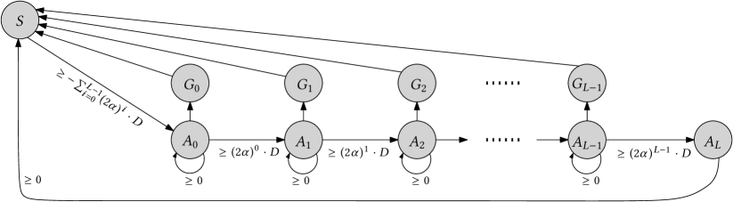
Figure 2: Plays as transitions between states. The gains for all plays avoiding states $G_{\ell}$ are given at the corresponding edges.

In Figure 2, we summarized the possible transitions between states, as described in Lemma 5, Lemma 6, and Lemma 7. Our goal is to show that if the game between an algorithm and the adversary starts at state $S$ and proceeds along described plays, then the total gain on all plays can be lower-bounded by a constant independent of the input sequence. It is worth observing that the total gain on a cycle $S\to A_{0}\to A_{1}\to\ldots A_{L-1}\to A_{L}\to S$ is non-negative (this corresponds to a scenario informally described in Section 3.2).

For a formal argument, for any state $q$, we introduce its potential $\Psi(q)$, defined as:

• $\Psi(S)=0$,

• $\Psi(A_{\ell})=-\sum_{i=\ell}^{L-1}(2\alpha)^{i}\cdot D$ for any $\ell\in\{0,\ldots,L\}$,

• $\Psi(G_{\ell})=-\sum_{i=\ell}^{L-1}(2\alpha)^{i}\cdot D+(1+\alpha)\cdot(2\alpha)^{\ell}\cdot D$ for any $\ell\in\{0,\ldots,L-1\}$.

We show that for any sequence of states starting at $S$ and ending at a state $q$, the total gain on all corresponding plays is at least $\Psi(q)$. To this end, we prove the following helper lemma.

Lemma 8.

Fix any play that starts at state $q_{a}$ and ends at state $q_{b}$, and let $T(q_{a},q_{b})$ be the play gain. Then, $T(q_{a},q_{b})\geq\Psi(q_{b})-\Psi(q_{a})$.

Proof.

We consider a few cases, depending on the state transition $q_{a}\to q_{b}$ and the corresponding play, cf. Figure 2.

• For a linear play, the only possible state transition is $S\to A_{0}$. By Lemma 5, $T(S,A_{0})\geq-\sum_{i=0}^{L-1}(2\alpha)^{i}\cdot D=\Psi(A_{0})-\Psi(S)$.

• For a bipartite play, the initial state is $A_{\ell}$, where $\ell\in\{0,\ldots,L-1\}$. We use Lemma 6 and consider three sub-cases. If the play ends at state $A_{\ell+1}$, then $T(A_{\ell},A_{\ell+1})\geq(2\alpha)^{\ell}\cdot D=\Psi(A_{\ell+1})-\Psi(A_{\ell})$. If it ends at state $A_{\ell}$, then $T(A_{\ell},A_{\ell})\geq 0=\Psi(A_{\ell})-\Psi(A_{\ell})$. Finally, if it ends at state $G_{\ell}$, then $T(A_{\ell},G_{\ell})\geq(1+\alpha)\cdot(2\alpha)^{\ell}\cdot D=\Psi(G_{\ell})-\Psi(A_{\ell})$.

• A finishing play always ends at $S$ and may start either at $A_{L}$ or at $G_{\ell}$, for $\ell\in\{0,\ldots,L-1\}$. In the former case, by Lemma 7, $T(A_{L},S)=(c+1)\cdot(2\alpha)^{L}\cdot D>0=\Psi(S)-\Psi(A_{L})$. In the latter case, the same lemma implies

  $$T(G_{\ell},S)+\Psi(G_{\ell})\geq \;(c+1)\cdot(3\alpha)\cdot(2\alpha)^{\ell}\cdot D-\sum_{i=\ell}^{L-1}(2\alpha)^{i}\cdot D+(1+\alpha)\cdot(2\alpha)^{\ell}\cdot D$$

  $$> \;\left((c+1)\cdot(3\alpha)-\frac{1}{1-2\alpha}+(1+\alpha)\right)\cdot(2\alpha)^{\ell}\cdot D$$

  $$> \;0=\Psi(S).$$

  The last inequality can be verified numerically: for $\alpha=1/(R_{0}-1)\approx 0.324$ and $c\geq c_{T}=2(R_{0}+1)/(R^{2}-2R_{0}-1)\approx 1.352$, it holds that $(c+1)\cdot 3\alpha-1/(1-2\alpha)+(1+\alpha)>0.768>0$.

Using the potentials and the lemma above, we may finally prove Theorem 2.

Proof of Theorem 2.

We consider an arbitrary sequence $\mathcal{I}$ of plays generated by the adversary in a way described in Section 3.5, Section 3.6 and Section 3.7. Let $S=q_{0},q_{1},\ldots,q_{r}$ be the induced sequence of states. Then, the total gain on sequence $\mathcal{I}$ is

$$\sum_{j=1}^{r}T(q_{j-1},q_{j})\geq\sum_{j=1}^{r}\left(\Psi(q_{j})-\Psi(q_{j-1})\right)=\Psi(q_{r})-\Psi(S)=\Psi(q_{r}),$$

which means that $C_{\textnormal{ALG}}(\mathcal{I})\geq(R_{0}-\varepsilon)\cdot C_{\textnormal{OPT}}(\mathcal{I})+\Psi(q_{r})$. For any state $q_{r}$, $\Psi(q_{r})\geq\Psi(A_{0})>-(1/(1-2\alpha))\cdot D$, and thus $C_{\textnormal{ALG}}(\mathcal{I})\geq(R_{0}-\varepsilon)\cdot C_{\textnormal{OPT}}(\mathcal{I})-(1/(1-2\alpha))\cdot D$.

As the minimum cost for Alg on any play is lower-bounded by a constant, the sequence $\mathcal{I}$ can be made arbitrarily costly for Alg, making the constant $(1/(1-2\alpha))\cdot D$ negligible, and showing that the competitive ratio of Alg is at least $R_{0}-\varepsilon$. As $\varepsilon$ can be made arbitrarily small by taking large values of parameters $L$ and $k$ (this also requires large value of $D$ as we assumed $D\geq k/c$), no algorithm operating in phases of fixed length, in the dynamic graph model, can achieve a competitive ratio lower than $R_{0}$.

One may wonder whether the dynamic graph model is essential to the presented proof and whether an adversary cannot simply generate the whole sequence on a larger but fixed graph. For a fixed graph however, nodes that were used in the previous plays become problematic in subsequent ones. To give a specific example, consider two consecutive bipartite plays, corresponding to state transitions $A_{\ell}\to A_{\ell+1}$ and $A_{\ell+1}\to A_{\ell+2}$, respectively. Right after the former play ends, both Alg and Opt have their files at nodes of set $Q$ of the former bipartite play, cf. Figure 1. Then, in the subsequent bipartite play, almost all nodes of $S$ lie in the middle of the way from Alg to Opt: this gives Alg an opportunity of moving its file towards the file of Opt, which is not captured by our current analysis.

Note on Mtlm performance: The proof of the lower bound on the competitive ratio for the algorithm Mtlm is a special case of the one presented above. We start the sequence in state $S$. After the linear play, the next state is $A_{0}$. Then, we may use bipartite play $L$ times arriving at state $A_{L}$, and finally the finishing play brings the game back to state $S$. Each play is a lower bound on the amortized performance of Mtlm (see the notes at the ends of Section 3.5, Section 3.6 and Section 3.7), and hence the amortized cost over such sequence of phases is at least $R_{0}-\varepsilon$ times the cost of Opt. But as the construction starts and ends in state $S$, the final and the initial potentials cancel out and the amortized cost of Mtlm over such sequence is equal to its actual cost. This implies that the competitive ratio of Mtlm is at least $R_{0}-\varepsilon$. As $\varepsilon$ can be made arbitrarily small, the ratio is at least $R_{0}$.

We note that for Mtlm the proof could be made even simpler: the game starts at state $S$, and then the adversary uses a linear play followed immediately by a finishing play. Again, as the sequence starts and ends in the same state, the amortized cost of Mtlm is equal to its actual cost, which implies the desired lower bound on its competitive ratio.

4 Linear Program for File Migration

In this section, we present a linear programming model for the analysis of both algorithm Mtlm by Bartal et al. [BCI01] and later for our algorithm Dlm. We also discuss how the former can be used for generating tight cases for Mtlm that we used as part of our lower bound construction in Section 3. Finally, we discuss how the LP was used to develop the combinatorial proof presented in Section 2.

4.1 LP Analysis of MTLM-like Algorithms

We start by analyzing an Mtlm-like algorithm Alg. We use our notation for distances from Section 2.1. Alg is a variant of Mtlm parameterized by two values $\beta$ and $\delta$. The length of its phase is $\delta\cdot D$ and the initial point of Alg is denoted by $A_{0}$. We denote the set of requests within a phase by $\mathcal{R}$. At the end of a phase, Alg migrates the file to a point $A_{1}$ that minimizes the function

$$f(x)=[A_{0},x]+\beta\cdot[x,\mathcal{R}].$$

As in the amortized analysis of the algorithm Mtlm [BCI01], we use a potential function equal to $\phi\cdot D$ times the distance between the files of Alg and Opt, where $\phi$ is a parameter used in the analysis. We let $O_{0}$ and $O_{1}$ denote the initial and final position of Opt during the studied phase, respectively. Then, the amortized cost of Alg in a single phase is $C_{\textnormal{ALG}}=\delta\cdot[A_{0},\mathcal{R}]+[A_{0},A_{1}]+\phi\cdot([A_{1},O_{1}]-[A_{0},O_{0}])$.

We observe that if in a given phase, the cost of Opt, denoted $C_{\textnormal{OPT}}$, is zero, then Opt does not move its file ($O_{0}=O_{1}$) and all requests are given at $O_{0}$. Moreover, Alg migrates the file to $O_{0}$, and thus $C_{\textnormal{ALG}}=(1+\delta-\phi)\cdot[A_{0},O_{0}]$. Therefore, Alg is competitive provided that $\phi\geq 1+\delta$ and from now on we assume that $C_{\textnormal{OPT}}>0$.

The following factor-revealing LP finds a worst-case instance for a single phase of Alg. Namely, it encodes inequalities that are true for any phase and a graph on which Alg can be run. The goal of the LP is to maximize the ratio between $C_{\textnormal{ALG}}$ and $C_{\textnormal{OPT}}$. As $C_{\textnormal{OPT}}>0$, an instance can be scaled: we set $C_{\textnormal{OPT}}=1$ and we maximize $C_{\textnormal{ALG}}$. Let $V=\{A_{0},A_{1},O_{0},O_{1}\}$ and $V^{\prime}=V\cup\{\mathcal{R}\}$. Basic variables used in the LP correspond to all pairwise distances between elements of $V^{\prime}$ multiplied by $D$, i.e., we use variables $[v_{i},v_{j}]$ for all pairs $v_{i},v_{j}\in V^{\prime}$.

$$\begin{array}[]{ll}\emph{maximize $C_{\textnormal{ALG}}$}&\\[3.00003pt] \emph{subject to:}&\\[1.99997pt] \quad C_{\textnormal{ALG}}=\delta\cdot[A_{0},\mathcal{R}]+[A_{0},A_{1}]+\phi\cdot([A_{1},O_{1}]-[A_{0},O_{0}])&\\[1.99997pt] \quad C_{\textnormal{OPT}}=1&\\[1.99997pt] \quad C_{\textnormal{OPT}}=C_{\textnormal{OPT}}^{\textnormal{req}}+C_{\textnormal{OPT}}^{\textnormal{move}}&\\[1.99997pt] \quad C_{\textnormal{OPT}}^{\textnormal{move}}\geq[O_{0},O_{1}]&\\[1.99997pt] \quad 2\cdot C_{\textnormal{OPT}}\geq\delta\cdot[O_{0},\mathcal{R}]+\delta\cdot[O_{1},\mathcal{R}]+(2-\delta)\cdot C_{\textnormal{OPT}}^{\textnormal{move}}&\\[1.99997pt] \quad f(A_{1})\leq f(v)&\text{for all }{v\in V}\\[1.99997pt] \quad 0\leq[v_{1},v_{3}]\leq[v_{1},v_{2}]+[v_{2},v_{3}]&\text{for all }v_{1},v_{2},v_{3}\in V^{\prime}\end{array}$$

In the LP above, $C_{\textnormal{OPT}}^{\textnormal{req}}$ and $C_{\textnormal{OPT}}^{\textnormal{move}}$ denote the cost of Opt for serving the request and the cost of Opt for migrating the file, respectively. The inequality $2\cdot C_{\textnormal{OPT}}\geq\delta\cdot[O_{0},\mathcal{R}]+\delta\cdot[O_{1},\mathcal{R}]+(2-\delta)\cdot C_{\textnormal{OPT}}^{\textnormal{move}}$ is guaranteed by Lemma 3. Finally, the LP encodes that distances between objects from $V^{\prime}=V\cup\{\mathcal{R}\}$ satisfy the triangle inequality.

For any choice of parameters $\beta$, $\delta$, and $\phi$, the LP above finds an instance that maximizes the competitive ratio of Alg. Note that such instance is not necessarily a certificate that Alg indeed performs poorly: in particular, inequalities that lower-bound the cost of Opt might not be tight. However, the opposite is true: if the value of $C_{\textnormal{ALG}}$ returned by the LP is $\xi$, then for any possible instance the ratio is at most $\xi$.

Let $c_{0}=1.841$ be the phase length of Mtlm. Setting $\delta=c_{0}$ and $\beta=\phi=1+c_{0}$ yields that the optimal value of the LP is $R_{0}\approx 4.086$, which can be interpreted as a numerical counterpart of the original analysis for Mtlm in [BCI01].

To reproduce a formal mathematical proof that the competitive ratio of Mtlm is at most $R_{0}$, we may appropriately combine inequalities from the LP. Given a feasible solution to the dual of the LP, it suffices to interpret the values of variables in the dual solution as coefficients in the combination of the primal constraints, i.e., each constraint in our LP is multiplied by the value of the corresponding dual variable and then all constraints are summed together. This would give a proof that the value of the objective function of our LP (the ratio of the amortized cost of Mtlm to the cost of Opt in a single phase) is at most the value of the dual solution. By the strong duality, if the coefficients are taken from an optimal dual solution, the obtained bound on the ratio is at most $R_{0}$. If we sum this property over all phases, this implies that Mtlm is $R_{0}$-competitive.

4.2 Studying LP Output for MTLM

The LP presented above allowed us to numerically find the “hard instances” for the amortized analysis of Mtlm, i.e., instances consisting of a single phase, on which the amortized cost of Mtlm is arbitrarily close to $R_{0}\cdot\textsc{Opt}$. LP returned three such instances, depicted in Figure 3. Two of them (called linear instances) were later generalized to the linear play (cf. Section 3.5) and the third (called bipartite instance) — to the bipartite play (cf. Section 3.6). An additional hard instance is the finishing play, which corresponds to the case $C_{\textnormal{OPT}}=0$ described in the previous section. All these adversarial plays were later used in our lower bound construction.

It is important to observe that while the LP always gives a correct upper bound for the Mtlm-to-Opt ratio, if we want to lower-bound this ratio, two issues need to be overcome. We discuss them on the example of the linear instance and later we indicate the necessary changes for the bipartite instance. In our description, we use $\alpha$ and $t$ as defined in Section 3, i.e., $\alpha=1/(R_{0}-1)$ and $t=1+1/R_{0}$.

Figure 3: Tight instances for the amortized analysis of Mtlm as returned by the LP: two linear instances on the left and the bipartite instance on the right. The distances to $\mathcal{R}$ represent the average distances to the requests of the phase.

The first issue is that the LP returns only the the average distance from particular points of $V=\{A_{0},A_{1},O_{0},O_{1}\}$ to the phase requests. One may think that the LP returns a metric space, with one of the points denoted $\mathcal{R}$: the distance from a point to $\mathcal{R}$ corresponds to the average distance from such point to phase requests. For an actual input, we need to distribute these requests so that the costs of Mtlm and Opt are unchanged. For example, in one of the linear instances (the bottom-left part of Figure 3), LP assumes that the metric space consists of three points. The outer points are at distance $1$: the first one contains the initial positions of Mtlm and Opt and the final position of Mtlm, and the second one — the final position of Opt. The inner point is $\mathcal{R}$, its distances to the outer points are $t/c_{0}\approx 0.676$ and $(c_{0}-t)/c_{0}\approx 0.324$, respectively. If we placed all requests at $\mathcal{R}$, then the cost of serving requests by Mtlm would be unchanged, but Mtlm would then migrate the file to $\mathcal{R}$ and not the the point $A_{1}$ returned by the LP. Thus, we need to (i) distribute the requests, so that their average distances to other metric points remain the same, (ii) ensure that the migration choices for Mtlm remain unchanged. For the linear play, this is simply achieved by placing $c_{0}-t$ requests at point $a$ and the remaining $t$ requests at point $b$.

The second issue is that the LP only lower-bounds the cost of Opt, and its actual cost might be in fact higher. (In other words, the inequalities in the proof of Lemma 3 may be strict.) Luckily, the structure of the examples returned by the LP makes it possible for the lower bound and the actual cost of Opt to coincide. In the linear play, this is achieved by placing initial $c_{0}-t$ requests at point $A_{0}=O_{0}$ and the subsequent $t$ requests at the second point.

Dealing with these issues is different for the LP output that constitutes the bipartite instance, depicted on the right side of Figure 3. The presented graph constitutes a tight example for Mtlm for any values of $d_{1}$ and $d_{2}$. Again, if we placed all requests at $\mathcal{R}$, then Mtlm would migrate its file to this point. To forbid this, we distribute the phase requests in a large set $S$, whose distances to points $A_{1}$ and $O_{0}$ are equal to $d_{2}$. This modification preserves the serving costs of Opt and Mtlm and it discourages Mtlm from migrating to any node from $S$. (Further modifications that we made for the bipartite play are designed to prevent any algorithm to migrate to nodes from $S$.)

4.3 LP Analysis of DLM-like Algorithms

Now we show how to adapt the LP from the previous section to analyze Dlm-type algorithms. Recall that after $1.75\,D$ requests, Dlm evaluates the geometry of the so-far-received requests and decides whether to continue this phase or not. Although the final parameters of Dlm are elegant numbers (multiplicities of 1/4), they were obtained by a tedious optimization process using the LP we present below. Furthermore, the LP below does not give us an explicit rule for continuing the phase; it only tells that Dlm is successful either in a short or in a long phase. We elaborate more about these issues in Section 4.4.

Recall that in a phase, Dlm considers three sets of requests $\mathcal{R}_{1}$, $\mathcal{R}_{2}$, and $\mathcal{R}_{3}$. Set $\mathcal{R}_{i}$ contains consecutive $\delta_{i}\cdot D$ requests, where $\delta_{i}$ is the parameter of Dlm. First, assume that Dlm always processes three parts and afterwards it moves the file to a point $A_{3}$ that minimizes the function

$$h(x)=[A_{0},x]+\beta_{1}\cdot[x,\mathcal{R}_{1}]+\beta_{2}\cdot[x,\mathcal{R}_{2}]+\beta_{3}\cdot[x,\mathcal{R}_{3}],$$

where $\beta_{i}$ are the parameters that we choose later. We denote the strategy of an optimal algorithm by OptL (short for Opt-Long). Let $O^{L}_{0}$, $O^{L}_{1}$, $O^{L}_{2}$ and $O^{L}_{3}$ denote the trajectory of OptL ($O^{L}_{0}$ is the initial position of the OptL’s file at the beginning of the phase, and $O^{L}_{i}$ is its position right after the $i$-th part of the phase). This time $V=\{A_{0},A_{3},O^{L}_{0},O^{L}_{1},O^{L}_{2},O^{L}_{3}\}$ and $V^{\prime}=V\cup\{\mathcal{R}_{1},\mathcal{R}_{2},\mathcal{R}_{3}\}$. Analogously to the previous section, we obtain the following LP.

$$\begin{array}[]{ll}\emph{maximize $C_{\textnormal{ALGL}}$}&\\[3.00003pt] \emph{subject to:}&\\[1.99997pt] \quad C_{\textnormal{ALGL}}=[A_{0},A_{3}]+\sum_{i=1,2,3}\delta_{i}\cdot[A_{0},\mathcal{R}_{i}]+\phi\cdot([A_{3},O^{L}_{3}]-[A_{0},O^{L}_{0}])&\\[1.99997pt] \quad C_{\textnormal{OPTL}}=1&\\[1.99997pt] \quad C_{\textnormal{OPTL}}=\sum_{i=1,2,3}\left(C_{\textnormal{OPTL}}^{\textnormal{req}}(i)+C_{\textnormal{OPTL}}^{\textnormal{move}}(i)\right)&\\[1.99997pt] \quad C_{\textnormal{OPTL}}^{\textnormal{move}}(i)\geq[O^{L}_{i-1},O^{L}_{i}]&\text{for }i=1,2,3\\[1.99997pt] \quad 2\cdot C_{\textnormal{OPTL}}(i)\geq\delta_{i}\cdot[O_{i-1}^{L},\mathcal{R}_{i}]+\delta_{i}\cdot[O_{i}^{L},\mathcal{R}_{i}]+(2-\delta_{i})\cdot C_{\textnormal{OPTL}}^{\textnormal{move}}(i)&\text{for }i=1,2,3\\[1.99997pt] \quad h(A_{3})\leq h(v)&\text{for all }{v\in V}\\[1.99997pt] \quad 0\leq[v_{1},v_{3}]\leq[v_{1},v_{2}]+[v_{2},v_{3}]&\text{for all }v_{1},v_{2},v_{3}\in V^{\prime}\end{array}$$

We note that such parameterization alone does not improve the competitive ratio, i.e., for any choice of parameters $\delta_{i}$ and $\beta_{i}$, the objective value of the LP above is at least $R_{0}\approx 4.086$.

However, as stated in Section 2.1, Dlm verifies if after two parts it can migrate its file to a point $A_{2}$ being the minimizer of the function

$$g(x)=[A_{0},x]+\beta^{\prime}_{1}\cdot[x,\mathcal{R}_{1}]+\beta^{\prime}_{2}\cdot[x,\mathcal{R}_{2}],$$

where $\beta^{\prime}_{i}$ are the parameters that we choose later.

In our analysis presented in Section 2, we gave an explicit rule whether the migration to $A_{2}$ should take place. However, for our LP-based approach, we follow a slightly different scheme. Namely, if the migration to $A_{2}$ guarantees that the amortized cost in the short phase (the first two parts) is at most $4$ times the cost of any strategy for the short phase, then Dlm may move to $A_{2}$ and we immediately achieve competitive ratio $4$ on the short phase. Otherwise, we may add additional constraints to the LP, stating that the competitive ratio of an algorithm which moves to $A_{2}$ is at least $4$ (against any chosen strategy OptS). Analogously to OptL, the trajectory of OptS is described by three points: $O^{S}_{0}$, $O^{S}_{1}$, and $O^{S}_{2}$. This allows us to strengthen our LP by adding the following inequalities:

$$\begin{array}[]{ll}C_{\textnormal{ALGS}}=[A_{0},A_{2}]+\sum_{i=1,2}\delta_{i}\cdot[A_{0},\mathcal{R}_{i}]+\phi\cdot([A_{2},O^{S}_{2}]-[A_{0},O^{S}_{0}])&\\[1.99997pt] C_{\textnormal{OPTS}}=\sum_{i=1,2}\left(C_{\textnormal{OPTS}}^{\textnormal{req}}(i)+C_{\textnormal{OPTS}}^{\textnormal{move}}(i)\right)&\\[1.99997pt] C_{\textnormal{OPTS}}^{\textnormal{move}}(i)\geq[O^{S}_{i-1},O^{S}_{i}]&\text{for }i=1,2\\[1.99997pt] 2\cdot C_{\textnormal{OPTS}}(i)\geq\delta_{i}\cdot[O_{i-1}^{S},\mathcal{R}_{i}]+\delta_{i}\cdot[O_{i}^{S},\mathcal{R}_{i}]+(2-\delta_{i})\cdot C_{\textnormal{OPTS}}^{\textnormal{move}}(i)&\text{for }i=1,2\\[1.99997pt] g(A_{2})\leq g(v)&\text{for all }{v\in V}\\[1.99997pt] C_{\textnormal{ALGS}}\geq 4\cdot C_{\textnormal{OPTS}}\end{array}$$

We also change $V$ to $\{A_{0},A_{2},A_{3},O^{L}_{0},O^{L}_{1},O^{L}_{2},O^{L}_{3},O^{S}_{0},O^{S}_{1},O^{S}_{2}\}$, both in new and in old inequalities.

When we choose $\phi=3$, fix phase length parameters to be $\delta_{1}=1$, $\delta_{2}=0.75$, $\delta_{3}=0.5$ and parameters for functions $g$ and $h$ to be $\beta^{\prime}_{1}=2$, $\beta^{\prime}_{2}=1$, $\beta_{1}=1,\beta_{2}=0.25$ and $\beta_{3}=0.75$, we obtain that the value of the above LP is $4$. Again, this can be interpreted as a numerical argument that Dlm is indeed 4-competitive.

4.4 From LP to Analytic Proof

Admittedly, the LP presented above does not lead directly to the algorithm Dlm and its proof presented in Section 2, although it can be used to achieve them in a quite streamlined fashion. First issue concerns the actual choice of parameters used in LP (coefficients $\phi,\delta_{1},\delta_{2},\delta_{3},\beta^{\prime}_{1},\beta^{\prime}_{2},\beta_{1},\beta_{2}$ and $\beta_{3}$). They were chosen semi-automatically using the grid search first and then fine-tuned using local search. Surprisingly, such approach yielded the objective value (bound on the competitive ratio) being an integer $4$, and we were not able to improve it further. Moreover, the optimized parameters also turned out to be “nice numbers” (rational numbers with small denominators).

As already observed, the dual variables in the optimal solution can be used in a formal proof for Dlm competitiveness. However, the dual variables returned by LP solvers were not round fractions. To alleviate this issue, we simplified the dual program by iteratively choosing a single constraint, dropping this constraint and verifying whether the objective value remains the same. The reduced dual LP still guaranteed the competitive ratio of $4$, but its simplified form allowed the LP solver to find a solution consisting only of “nice numbers” (multiplicities of $1/4$).

Finally, the proof that we obtained, by summing up the LP inequalities multiplied by the dual solution values, naturally decomposes into two parts: one corresponding to the long phase and one corresponding to the short phase. The short phase part, when summed up, gives rise to a single inequality. This inequality encompasses the key property of the scenarios where the long phase should be chosen. It therefore describes the decision rule used in the algorithm Dlm.

5 Conclusions

While in the last decade factor-revealing LPs became a standard tool for analysis of approximation algorithms, their application to online algorithms so far have been limited to online bipartite matching and its variants (see, e.g., [MSVV07, MY11]) and for showing lower bounds [ACR17]. In this paper, we successfully used the factor-revealing LP to bound the competitive ratio of an algorithm for an online problem defined on an arbitrary metric space. We believe that similar approaches could yield improvements also for other online graph problems.

References

- [ABF93a] Baruch Awerbuch, Yair Bartal, and Amos Fiat. Competitive distributed file allocation. In Proc. 25th ACM Symp. on Theory of Computing (STOC), pages 164–173, 1993.
- [ABF93b] Baruch Awerbuch, Yair Bartal, and Amos Fiat. Heat & Dump: Competitive distributed paging. In Proc. 34th IEEE Symp. on Foundations of Computer Science (FOCS), pages 22–31, 1993.
- [ABF98] Baruch Awerbuch, Yair Bartal, and Amos Fiat. Distributed paging for general networks. Journal of Algorithms, 28(1):67–104, 1998.
- [ACR17] Yossi Azar, Ilan Reuven Cohen, and Alan Roytman. Online lower bounds via duality. In Proc. 28th ACM-SIAM Symp. on Discrete Algorithms (SODA), pages 1038–1050, 2017.
- [AK95] Susanne Albers and Hisashi Koga. Page migration with limited local memory capacity. In Proc. 4th Int. Workshop on Algorithms and Data Structures (WADS), pages 147–158, 1995.
- [Bar95] Yair Bartal. Competitive Analysis of Distributed On-line Problems — Distributed Paging. PhD thesis, Tel-Aviv University, 1995.
- [Bar96] Yair Bartal. Distributed paging. In Dagstul Workshop on On-line Algorithms, pages 97–117, 1996.
- [BBK+94] Shai Ben-David, Allan Borodin, Richard M. Karp, Gabor Tardos, and Avi Wigderson. On the power of randomization in online algorithms. Algorithmica, 11(1):2–14, 1994.
- [BBKM09] Marcin Bienkowski, Jaroslaw Byrka, Miroslaw Korzeniowski, and Friedhelm Meyer auf der Heide. Optimal algorithms for page migration in dynamic networks. Journal of Discrete Algorithms, 7(4):545–569, 2009.
- [BCI01] Yair Bartal, Moses Charikar, and Piotr Indyk. On page migration and other relaxed task systems. Theoretical Computer Science, 268(1):43–66, 2001. Also appeared in Proc. of the 8th SODA, pages 43–52, 1997.
- [BE98] Allan Borodin and Ran El-Yaniv. Online Computation and Competitive Analysis. Cambridge University Press, 1998.
- [BFR95] Yair Bartal, Amos Fiat, and Yuval Rabani. Competitive algorithms for distributed data management. Journal of Computer and System Sciences, 51(3):341–358, 1995.
- [Bie12] Marcin Bienkowski. Migrating and replicating data in networks. Computer Science — Research and Development, 27(3):169–179, 2012.
- [BS89] David L. Black and Daniel D. Sleator. Competitive algorithms for replication and migration problems. Technical Report CMU-CS-89-201, Department of Computer Science, Carnegie-Mellon University, 1989.
- [CLRW97] Marek Chrobak, Lawrence L. Larmore, Nick Reingold, and Jeffery Westbrook. Page migration algorithms using work functions. Journal of Algorithms, 24(1):124–157, 1997.
- [GS90] Bezalel Gavish and Olivia R. Liu Sheng. Dynamic file migration in distributed computer systems. Communications of the ACM, 33(2):177–189, 1990.
- [IW91] Makoto Imase and Bernard M. Waxman. Dynamic Steiner tree problem. SIAM Journal on Discrete Mathematics, 4(3):369–384, 1991.
- [LRWY99] Carsten Lund, Nick Reingold, Jeffery Westbrook, and Dicky C. K. Yan. Competitive on-line algorithms for distributed data management. SIAM Journal on Computing, 28(3):1086–1111, 1999.
- [Mat08] Akira Matsubayashi. Uniform page migration on general networks. International Journal of Pure and Applied Mathematics, 42(2):161–168, 2008.
- [Mat15a] Akira Matsubayashi. A 3+Omega(1) lower bound for page migration. In Proc. 3rd Int. Symp. on Computing and Networking (CANDAR), pages 314–320, 2015.
- [Mat15b] Akira Matsubayashi. Asymptotically optimal online page migration on three points. Algorithmica, 71(4):1035–1064, 2015.
- [Mat16] Amanj Khorramian Akira Matsubayashi. Uniform page migration problem in euclidean space. Algorithms, 9(3), 2016.
- [MMVW97] Bruce M. Maggs, Friedhelm Meyer auf der Heide, Berthold Vöcking, and Matthias Westermann. Exploiting locality for data management in systems of limited bandwidth. In Proc. 38th IEEE Symp. on Foundations of Computer Science (FOCS), pages 284–293, 1997.
- [MSVV07] Aranyak Mehta, Amin Saberi, Umesh V. Vazirani, and Vijay V. Vazirani. Adwords and generalized online matching. Journal of the ACM, 54(5), 2007.
- [MVW99] Friedhelm Meyer auf der Heide, Berthold Vöcking, and Matthias Westermann. Provably good and practical strategies for non-uniform data management in networks. In Proc. 7th European Symp. on Algorithms (ESA), pages 89–100, 1999.
- [MY11] Mohammad Mahdian and Qiqi Yan. Online bipartite matching with random arrivals: an approach based on strongly factor-revealing LPs. In Proc. 43rd ACM Symp. on Theory of Computing (STOC), pages 597–606, 2011.
- [Wes94] Jeffery Westbrook. Randomized algorithms for the multiprocessor page migration. SIAM Journal on Computing, 23:951–965, 1994.