Classical and Quantum Logics with Multiple and a Common Lattice Models

Abstract

We consider a proper propositional quantum logic and show that it has multiple disjoint lattice models, only one of which is an orthomodular lattice (algebra) underlying Hilbert (quantum) space. We give an equivalent proof for the classical logic which turns out to have disjoint distributive and non-distributive ortholattices as its models. In particular, we prove that quantum as well as classical logics are complete and sound with respect to these lattices. We also show that there is one common non-orthomodular lattice that is a model of both quantum and classical logics. In technical terms, that enables us to run the same classical logic on both a digital (standard, two subset, 0-1 bit) computer and on a non-digital (say, a six subset) computer (with appropriate chips and circuits). With quantum logic, the same six element common lattice can serve us as a benchmark for an efficient evaluation of equations of bigger lattice models or theorems of the logic.

I Introduction: Is Logic Empirical?

In his seminal paper Is Logic Empirical? Putnam (1969), Hilary Putnam argues that logic we make use of to handle the statements and propositions of the theories we employ to describe the world around us is uniquely determined by it. “Logic is empirical. It makes … sense to speak of ‘physical logic’. We live in a world with a non-classical logic [of subspaces of the quantum Hilbert space $\mathcal{H}$ which form an orthomodular (non-distributive, non-Boolean) lattice]. Certain statements—just the ones we encounter in daily life—do obey classical logic, but this is so because the corresponding subspaces of $\mathcal{H}$ form a Boolean lattice.” (Putnam, 1969, Ch. V)

We see that Putnam, in effect, reduces the logics to lattices, while they should only be their models. “[We] just read the logic off from the Hilbert space $\mathcal{H}$.” (Putnam, 1969, Ch. III) This technical approach has often been adopted in both classical and quantum logics. In classical logic, it has been known as two-valued interpretation for more than a century. In quantum logic, since G. Birkhoff and J. von Neumann introduced it in 1935 Birkhoff and von Neumann (1936) and it is still embraced by many authors Wilce (Fall 2012). Subsequently, varieties of relational logic formulations, which closely follow lattice ordering relations, have been developed, e.g., by Dishkant Dishkant (1972), Goldblatt Goldblatt (1974), Dalla Chiara Dalla Chiara (1986), Nishimura Nishimura (1980, 2009), Mittelstaedt Mittelstaedt (1978), Stachow Stachow (1976), and Pták and Pulmannová Pták and Pulmannová (1991). More recently, Engesser and Gabbay Engesser and Gabbay (2002) made related usage of non-monotonic consequence relation, Rawling and Selesnick Rawling and Selesnick (2000) of binary sequent, Herbut Herbut (2012) of state-dependent implication of lattice of projectors in the Hilbert space, Tylec and Kuś Tylec and Kuś (2015) of partially ordered set (poset) map, Bikchentaev, Navara, and Yakushev Bikchentaev et al. (2015) of poset binary relation.

Another version of Birkhoff-von-Neumann style of viewing propositions as projections in Hilbert space rather than closed subspaces and their lattices as in the original Birkhoff-von Neumann paper has been introduced by Engesser, Gabbay, and Lehmann Engesser et al. (2007). Recently, other versions of quantum logics have been developed, such as a dynamic quantum logic by Baltag and Smets Baltag and Smets (2005, 2011), exogenous quantum propositional logic by Mateus and Sernadas Mateus and Sernadas (2006), a categorical quantum logic by Abramsky and Duncan Abramsky and Duncan (2006); Abramsky and Coecke (2004), and a projection orthoalgebraic approach to quantum logic by Harding Harding (2009).

However, we are interested in non-relational logics which combine propositions according to a set of true formulas/axioms and rules imposed on them. The propositions correspond to statements from a theory, say classical or quantum mechanics, and are not directly linked to particular measurement values. Such logics employ models which evaluate a particular combination of propositions and tell us whether it is true or not. Evaluation means mapping from a set of logic propositions to an algebra, e.g., a lattice, through which a correspondence with measurement values emerges, but indirectly. Therefore we shall consider a classical and a quantum logic defined as a set of axioms whose Lindenbaum-Tarski algebras of equivalence classes of expressions from appropriate lattices correspond to the models of the logics. Let us call such a logic an axiomatic logic.

We show that an axiomatic logic is wider than its relational logic variety in the sense of having many possible models and not only distributive ortholattice (Boolean algebra) for the classical logic and not only orthomodular lattice for the quantum logic. We make use of Hilbert-Ackermann’s presentation Hilbert and Ackermann (1950) of axiomatic classical logic in the schemata form and of Kalmbach’s axiomatic quantum logic Kalmbach (1983, 1974) (in Megill-Pavičić Pavičić and Megill (1999, 2009) presentation, i.e., without Kalmbach’s A1,A11 & A15 axioms which we prove redundant in Pavičić and Megill (1998a)), as typical examples of axiomatic logics.

It is well-known that there are many interpretations of the classical logic, e.g., two-valued, general Boolean algebra (distributive ortholattice), set-valued ones, etc. (Schechter, 2005, Ch. 8,9). These different interpretations are tantamount to different models of the classical logic and in this paper and several previous papers of ours we show that they are enabled by different definitions of the relation of equivalence for its different Lindenbaum-Tarski algebras. One model of the classical logic is a distributive numerically valued, mostly two-valued, lattice, while the others are non-distributive non-orthomodular lattices, one of them being the so-called O6 lattice, which can also be given set-valuations (Schechter, 2005, Ch. 8,9).

As for quantum logic, one of its models is an orthomodular lattice, while others are non-orthomodular lattices, one of them being again O6—the common model of both logics.

Within a logic we establish a unique deduction of all logic theorems from valid algebraic equations in a model and vice versa by proving the soundness and completeness of logic with respect to a chosen model. That means that we can infer the distributivity or orthomodularity in one model and disprove them in another by means of the same set of logical axioms and theorems. We can also consider O6 in which both the distributivity and orthomodularity fail; however, particular non-distributive and non-orthomodular conditions pass O6 only to map into the distributivity and orthomodularity through classical and quantum logics in other models of these logics.

We see that logic is at least not uniquely empirical since it can simultaneously describe distinct realities.

The paper is organised as follows. In Sec. II we define classical and quantum logics. In Sec. III we introduce distributive (ortho)lattices and orthomodular lattices as well as two non-distributive (one is O6) and four non-orthomodular ones (one is again O6), all of which are our models for classical and quantum logic, respectively. In Subec. IV.1, we prove soundness and in Subec. IV.2 completeness of classical and quantum logics with respect to the models introduced in Sec.III. In Sec. V, we discuss the obtained results.

II Logics

We consider logic ($\mathcal{L}$) to be a language which is defined by a set of conditions (axioms) and rules imposed on propositions. axioms and the rules of inference. We shall consider quantum as well as classical axiomatic logics.

The propositions in our axiomatic logic ($\mathcal{L}$) are well-formed formulae (wffs), which we define as follows.

Primitive (elementary) propositions are denoted as $p_{0},p_{1},p_{2},...$; primitive connectives are $\neg$ (negation) and $\vee$ (disjunction). $p_{j}$ is a wff for $j=0,1,2,...$; $\neg A$ is a wff if $A$ is a wff; $A\vee B$ is a wff if $A$ and $B$ are wffs.

We define operations as follows.

Definition II.1

(Conjunction)

$$\qquad A\wedge B\ {\buildrel\rm def\over{=}}\ \neg(\neg A\vee\neg B).$$

Definition II.2

(Classical implication)

$$\qquad A\to_{\rm c}B\ {\buildrel\rm def\over{=}}\ \neg A\vee B.$$

Definition II.3

(Kalmbach’s implication)

$$\qquad A\to_{3}B\ \ {\buildrel\rm def\over{=}}\ \ (\neg A\wedge\neg B)\vee(\neg A\wedge B)\vee(A\wedge(\neg A\vee B)).\quad$$

Definition II.4

(Quantum equivalence)

$$\qquad A\equiv_{q}B\ \ {\buildrel\rm def\over{=}}\ \ (\neg A\wedge\neg B)\vee(A\wedge B).$$

Definition II.5

(Classical Boolean equivalence)

$$\qquad A\equiv_{\rm c}B\ \ {\buildrel\rm def\over{=}}\ \ (B\to_{\rm c}A)\wedge(A\to_{\rm c}B).$$

Connectives bind in the following order $\to$, $\equiv$, $\vee$, $\wedge$, $\neg$, from weakest to strongest.

$\mathcal{F}^{\circ}$ is a set of all wffs. Algebra ${\mathcal{F}}=\langle{\mathcal{F}}^{\circ},\neg,\vee\rangle$ is built within $\mathcal{L}$ with wffs containing $\vee$ and $\neg$ by means of a set of axioms and rules of inference. In that way we get other expressions called theorems (axioms are also theorems). We make use of symbol $\vdash$ to denote the set of theorems; therefore $A\in\ \vdash$ means that $A$ is a theorem; it can also be written as $\vdash A$. We read it as: “$A$ is provable,” to mean: if $A$ is a theorem, then there is a proof of it. We present our systems of axioms in the schemata form, so that we do not have to make use of the rule of substitution.

Definition II.6

For $\Gamma\subseteq{\mathcal{F}}^{\circ}$, $A$ is derivable from $\Gamma$: $\Gamma\vdash_{\mathcal{L}}A$ (or simply $\Gamma\vdash A$) if there is a finite sequence of wffs, the last one of which is $A$, and every one of them is either an axiom of $\mathcal{L}$ or a member of $\Gamma$ or obtained from its precursors by means of the rule of inference of $\mathcal{L}$.

II.1 Classical Logic

In the classical logic $\mathcal{CL}$, the sign $\vdash_{\mathcal{CL}}$ denotes provability from the axioms via the rule of inference. We shall drop the subscript when it follows from context, e.g., in the following axioms and the rule of inference that define $\mathcal{CL}$.

Axioms

$${\rm A1}\qquad \vdash A\vee A\to_{c}A$$ (1)

$${\rm A2}\qquad \vdash A\to_{c}B\vee A$$ (2)

$${\rm A3}\qquad \vdash B\vee A\to_{c}A\vee B$$ (3)

$${\rm A4}\qquad \vdash(A\to_{c}B)\to_{c}(C\vee A\to_{c}C\vee B)$$ (4)

Rule of Inference (traditionally called Modus Ponens)

$${\rm R1}\qquad \vdash A\qquad\&\qquad A\to_{c}B\qquad\Rightarrow\qquad\vdash B$$ (5)

No particular valuations of the primitive propositions wffs consist of are assumed. We are only interested in whether wffs that are valid, i.e., true under all possible valuations of the underlying models. We show that the wffs that can be inferred from the axioms by means of the rule inference are exactly those that are valid by proving the soundness and completeness of the logic.

II.2 Quantum Logic

Quantum logic ($\mathcal{QL}$) is defined as a language consisting of propositions and connectives (operations) as introduced above, and the following axioms and a rule of inference. We will use $\vdash_{\mathcal{QL}}$ to denote provability from the axioms and the rule of $\mathcal{QL}$ and omit the subscript when it is obvious from the context, e.g., in the list of axioms and the rule of inference that follow.

Axioms

$${\rm A2}\qquad \vdash A\equiv_{q}B\rightarrow_{c}(B\equiv_{q}C\rightarrow_{c}A\equiv_{q}C)$$ (6)

$${\rm A3}\qquad \vdash A\equiv_{q}B\rightarrow_{c}\neg A\equiv_{q}\neg B$$ (7)

$${\rm A4}\qquad \vdash A\equiv_{q}B\rightarrow_{c}A\wedge C\equiv_{q}B\wedge C$$ (8)

$${\rm A5}\qquad \vdash A\wedge B\equiv_{q}B\wedge A$$ (9)

$${\rm A6}\qquad \vdash A\wedge(B\wedge C)\equiv_{q}(A\wedge B)\wedge C$$ (10)

$${\rm A7}\qquad \vdash A\wedge(A\vee B)\equiv_{q}A$$ (11)

$${\rm A8}\qquad \vdash\neg A\wedge A\equiv_{q}(\neg A\wedge A)\wedge B$$ (12)

$${\rm A9}\qquad \vdash A\equiv_{q}\neg\neg A$$ (13)

$${\rm A10}\qquad \vdash\neg(A\vee B)\equiv_{q}\neg A\wedge\neg B$$ (14)

$${\rm A12}\qquad \vdash(A\equiv_{q}B)\equiv_{q}(B\equiv_{q}A)$$ (15)

$${\rm A13}\qquad \vdash A\equiv_{q}B\rightarrow_{c}(A\rightarrow_{c}B)$$ (16)

$${\rm A14}\qquad \vdash(A\to_{c}B)\to_{3}(A\to_{3}(A\to_{3}B))$$ (17)

Rule of Inference

$$\ {\rm R1}\qquad \vdash A\quad\&\quad\vdash A\rightarrow_{3}B\quad\Rightarrow\quad\vdash B$$ (18)

Soundness and completeness for quantum logic we prove below show that the theorems which can be inferred from A1-14 via R1 are exactly those that are valid.

III Lattices

For the presentation of the main result it would be pointless and definitely unnecessary complicated to work with the full-fledged models, i.e., Hilbert space, and the new non-Hilbert models that would be equally complex. It would be equally too complicated to present complete quantum or classical logic of the second order with all the quantifiers. Instead, we shall deal with lattices and the propositional logics we introduced in Sec. II. We start with a general lattice which contains all the other lattices we shall use later on. The lattice is called an ortholattice and we shall first briefly present how one arrives at it starting with Hilbert space.

A Hilbert lattice is a kind of orthomodular lattice (see Def. III.5). In it the operation meet, $a\cap b$, corresponds to set intersection, ${\mathcal{H}}_{a}\bigcap{\mathcal{H}}_{b}$ of subspaces ${\mathcal{H}}_{a}$ and ${\mathcal{H}}_{b}$ of the Hilbert space ${\mathcal{H}}$; the ordering relation $a\leq b$ corresponds to ${\mathcal{H}}_{a}\subseteq{\mathcal{H}}_{b}$; the operation join, $a\cup b$, corresponds to the smallest closed subspace of $\mathcal{H}$ containing ${\mathcal{H}}_{a}\bigcup{\mathcal{H}}_{b}$; and the orthocomplement $a^{\prime}$ corresponds to ${\mathcal{H}}_{a}^{\perp}$, the set of vectors orthogonal to all vectors in ${\mathcal{H}}_{a}$. Within the Hilbert space there is the operation ${\mathcal{H}}_{a}+{\mathcal{H}}_{b}$ (sum of two subspaces); it is defined as as the set of sums of vectors from ${\mathcal{H}}_{a}$ and ${\mathcal{H}}_{b}$ but it has no a parallel in the Hilbert lattice. The following ${\mathcal{H}}_{a}+{\mathcal{H}}_{a}^{\perp}={\mathcal{H}}$ holds.

One can define all the lattice operations on the Hilbert space itself following the above definitions (${\mathcal{H}}_{a}\cap{\mathcal{H}}_{b}={\mathcal{H}}_{a}\bigcap{\mathcal{H}}_{b}$, etc.). Thus we have ${\mathcal{H}}_{a}\cup{\mathcal{H}}_{b}=\overline{{\mathcal{H}}_{a}+{\mathcal{H}}_{b}}=({\mathcal{H}}_{a}+{\mathcal{H}}_{b})^{\perp\perp}=({\mathcal{H}}_{a}^{\perp}\bigcap{\mathcal{H}}_{b}^{\perp})^{\perp}$, (Isham, 1995, p. 175) where $\overline{{\mathcal{H}}_{c}}$ is the closure of ${\mathcal{H}}_{c}$, and therefore ${\mathcal{H}}_{a}+{\mathcal{H}}_{b}\subseteq{\mathcal{H}}_{a}\cup{\mathcal{H}}_{b}$. For a finite dimensional ${\mathcal{H}}$ or for the orthogonal closed subspaces ${\mathcal{H}}_{a}$ and ${\mathcal{H}}_{b}$ we have ${\mathcal{H}}_{a}+{\mathcal{H}}_{b}={\mathcal{H}}_{a}\cup{\mathcal{H}}_{b}$. (Halmos, 1957, pp. 21-29), (Kalmbach, 1983, pp. 66,67), (Mittelstaedt, 1978, pp. 8-16).

For vector $x\in{\mathcal{H}}$ that has a unique decomposition $x=y+z$ for $y\in{\mathcal{H}}_{a}$ and $z\in{\mathcal{H}}_{a}^{\perp}$ there is a projection $P_{a}(x)=y$ associated with ${\mathcal{H}}_{a}$. The closed subspace which belong to $P$ is ${\mathcal{H}}_{P}=\{x\in{\mathcal{H}}|P(x)=x\}$. Let $P_{a}\cap P_{b}$ denote a projection on ${\mathcal{H}}_{a}\cap{\mathcal{H}}_{b}$, $P_{a}\cup P_{b}\>$ a projection on ${\mathcal{H}}_{a}\cup{\mathcal{H}}_{b}$, $P_{a}+P_{b}\>$ a projection on ${\mathcal{H}}_{a}+{\mathcal{H}}_{b}\>$ if ${\mathcal{H}}_{a}\perp{\mathcal{H}}_{b}$, and let $P_{a}\leq P_{b}$ means ${\mathcal{H}}_{a}\subseteq{\mathcal{H}}_{b}$. Then $a\cap b$ corresponds to $P_{a}\cap P_{b}=\lim_{n\to\infty}(P_{a}P_{b})^{n}$,(Mittelstaedt, 1978, p. 20) $a^{\prime}$ to $I-P_{a}$, $a\cup b$ to $P_{a}\cup P_{b}=I-\lim_{n\to\infty}[(I-P_{a})(I-P_{b})]^{n}$,(Mittelstaedt, 1978, p. 21) and $a\leq b$ to $P_{a}\leq P_{b}$. $a\leq b$ also corresponds to either $P_{a}=P_{a}P_{b}$ or to $P_{a}=P_{b}P_{a}$ or to $P_{a}-P_{b}=P_{a\cap b^{\prime}}$. Two projectors commute iff their associated closed subspaces commute. This means that $a\cap(a^{\prime}\cup b)\leq b$ corresponds to $P_{a}P_{b}=P_{b}P_{a}$. In the latter case we have: $P_{a}\cap P_{b}=P_{a}P_{b}$ and $P_{a}\cup P_{b}=P_{a}+P_{b}-P_{a}P_{b}$. $a\perp b$, i.e., $P_{a}\perp P_{b}$ is characterised by $P_{a}P_{b}=0$. (Isham, 1995, pp. 173-176), (Kalmbach, 1983, pp. 66,67), (Mittelstaedt, 1978, pp. 18-21), (Holland, Jr., 1970, pp. 47-50),

Closed subspaces ${\mathcal{H}}_{a}$,${\mathcal{H}}_{b}$,… as well as the corresponding projectors $P_{a}$,$P_{b}$,…  form an algebra called the Hilbert lattice which is an ortholattice. The conditions of the following definition can be easily read off from the properties of the aforementioned Hilbert subspaces or projectors.

Definition III.1

An ortholattice (OL) is an algebra $\langle{\mathcal{OL}}_{0},^{\prime},\cup,\cap\rangle$ in which for any $a,b,c\in\,{\mathcal{OL}}_{0}$ Megill and Pavičić (2002) the following conditions hold

$$a^{\prime\prime}\>=\>a$$ (19)

$$a\cup(a\cap b)\>=\>a$$ (20)

$$a\cup b\>=\>b\cup a$$ (21)

$$a\cap b\>=\>(a^{\prime}\cup b\,^{\prime})^{\prime}$$ (22)

$$a\cup(b\cup b\,^{\prime})\>=\>b\cup b\,^{\prime}$$ (23)

$$(a\cup b)\cup c\>=\>a\cup(b\cup c)$$ (24)

Since $b\cup b^{\prime}=a\cup a\,^{\prime}$ for any $a,b\in\,{\mathcal{OL}}_{0}$, we define the least and the greatest elements of the lattice:

$$\rm\textstyle{0}\,{\buildrel\rm def\over{=}}a\cap a^{\prime},\qquad\qquad\qquad\textstyle{1}\,{\buildrel\rm def\over{=}}a\cup a^{\prime},$$ (25)

and the ordering relation ($\leq$) on the lattice:

$$\qquad a\leq b\ \quad{\buildrel\rm def\over{\Longleftrightarrow}}\quad\ a\cap b=a\quad\Longleftrightarrow\quad a\cup b=b,\qquad$$ (26)

Definition III.2

(Sasaki hook)

$$a\to_{1}b\ \ {\buildrel\rm def\over{=}}\ \ a^{\prime}\cup(a\cap b)$$ (27)

Definition III.3

(Quantum equivalence)

$$a\equiv_{q}b\ \ {\buildrel\rm def\over{=}}\ \ (a\cap b)\cup(a^{\prime}\cap b\,^{\prime}).$$ (28)

Definition III.4

(Classical equivalence)

$$a\equiv_{c}b\ \ {\buildrel\rm def\over{=}}\ \ (a^{\prime}\cup b)\cap(b\,^{\prime}\cup a).$$ (29)

Connectives bind in the following order $\to$, $\equiv$, $\cup$, $\cap$, and ^′, from weakest to strongest.

Definition III.5

(Pavičić, Pavičić (1993).) An orthomodular lattice (OML) is an OL in which condition (30) (called orthomodularity) holds

$$a\equiv_{q}b=1\qquad\Rightarrow\qquad a=b.$$ (30)

Every Hilbert space (finite and infinite) and every phase space is orthomodular.

Definition III.6

(Pavičić, Pavičić (1998).) A distributive ortholattice (DL) (also called a Boolean algebra) is an OL in which condition (31) (called distributivity) holds

$$a\equiv_{c}b=1\qquad\Rightarrow\qquad a=b.$$ (31)

Every phase space is distributive and, of course, orthomodular since every distributive ortholattice is orthomodular.

The opposite directions of meta-implications in Eqs. (30) and (31) hold in any OL.

Definition III.7

(Pavičić and Megill, Pavičić and Megill (1999).) A weakly orthomodular ortholattice (WOML) is an OL in which either of conditions (32,33) (called weak orthomodularity) hold

$$a\to_{1}b=\textstyle{1}\qquad \Rightarrow \qquad b^{\prime}\to_{1}a^{\prime}=\textstyle{1},$$ (32)

$$a\equiv b=1\qquad \Rightarrow \qquad(a\cup c)\equiv(b\cup c)=1.\qquad$$ (33)

Definition III.8

(Pavičić, this paper.) A WOML1 is a WOML in which

$$[(a\to_{1}b)\equiv(b\to_{1}a)]\ =\ (a\equiv b)$$ (34)

holds.

Definition III.9

(Pavičić, this paper.) A WOML2 is a WOML1 in which

$$[(a\equiv b)^{\prime}\to_{1}a^{\prime}]\ =\ (a\to_{1}b)$$ (35)

holds.

Definition III.10

(Pavičić, this paper.) A WOML* is a WOML in which neither Eq. (30), nor (35), nor (34) hold.

Definition III.11

(Pavičić and Megill, Pavičić and Megill (1999, 2008).) A weakly distributive ortholattice (WDL) is an OL in which condition (36) (called commensurability) holds

$$(a\cap b)\cup(a\cap b^{\prime})\cup(a^{\prime}\cap b)\cup(a^{\prime}\cap b^{\prime})=1.$$ (36)

Definition III.12

(Pavičić and Megill, Pavičić and Megill (1999).) A weakly distributive ortholattice (WDL) is a WOML in which condition (37) (called weak distributivity) holds

$$a\cup(b\cap c)\equiv_{c}(a\cup b)\cap(a\cup c)=1.$$ (37)

Definitions III.11 and III.12 are equivalent. We give both definitions here in order to, on the one hand, stress that a WDL is a lattice in which all variables are commensurable and, on the other, to show that in WDL the distributivity holds only in its weak form given by Eq. (37) which we will use later on.

Definition III.13

(Pavičić and Megill, Pavičić and Megill (2008)) A WDL* is a WDL in which Eq. (31) does not hold.

We represent finite lattices by a Hasse diagrams which consist of vertices (dots) and edges (lines that connect dots). Each dot represents an element in a lattice, and positioning an element $a$ above another element $b$ and connecting them by a line means $a\leq b$. E.g., in Fig. 1 (a) we have $0\leq x\leq y\leq 1$. There, for instance, $x$ is not in a relation with either $x^{\prime}$ or $y^{\prime}$.

The statement “orthomodularity (30) does not hold in WOML*” reads $\sim\!\!\![(\forall a,b\in{\rm WOML}*)((a\!\equiv\!b=1)\ \Rightarrow\ (a=b))]$ what we can write as $(\exists a,b\!\!\in\!\!{\rm WOML}*)(a\!\!\equiv\!\!b\!=\!1\ \&\ a\neq b)$, where “$\sim$” is a meta-negation and “$\&$” a meta-conjuction. An example of a WOML* is O6 from Fig. 1 (a) and we can easily check the statement on it. O6 is also an example of a WDL* and we can verify the statement “distributivity (31) does not hold in WDL*” on it, as well. Similarly, “condition (35) does not hold in WOML*” we can write as $(\exists a,b\!\in\!{\rm WOML}*)(((a\!\equiv\!b)^{\prime}\to_{1}a^{\prime})\ \neq\ (a\to_{1}b))$.

Figure 1: (a) O6; (b) O7 (Beran, Fig. 7b Beran (1985)); (c) O8 (Rose-Wilkinson-1 Megill and Pavičić (2003))

Definition III.14

(Pavičić, this paper.) A WOML1* is a WOML1 in which neither Eq. (30) nor (35) hold.

An example of a WOML1* is O7 from Fig. 1 (b).

Definition III.15

(Pavičić, this paper.) A WOML2* is a WOML2 in which Eq. (30) does not hold.

An example of a WOML2* is O8 from Fig. 1 (c).

Lemma III.1

OML is properly included in (i.e., it is stronger than) WOML2, WOML2 is properly included in WOML1, and WOML1 is properly included in WOML,

Proof. Eq. (32) passes O6, O7, and O8 from Fig. 1. Eq. (34) passes O7 and O8, but fails in O6. Eq. (35) passes O8 but fails in both O6 and O7. Eq. (30) fails in O6, O7, and O8. To find the failures and passes we used our program lattice McKay et al. (2000).   $\blacksquare$

Lemma III.2

OML is included in neither WOML2*, nor WOML1*, nor WOML*. WOML2* is included in neither WOML1*, nor WOML*. WOML1* is not included in WOML*.

Proof. The proof straightforwardly follows from the one of Lemma III.1 and the definitions of WOML*, WOML1*, WOML2*, and OML.   $\blacksquare$

According to Definitions III.10, III.14, III.15, and III.13, of WOML*, WOML1*, WOML2*, and WDL*, respectively, these lattices denote set-theoretical differences and that is going to play a crucial role in our proofs of completeness in Subsection IV.2 in contrast to Pavičić and Megill (1999) where we considered only WOML without excluding the orthomodular equation. In Subsection IV.2 we shall come back to this decisive difference between the two approaches. Note that the set-differences are not equational varieties. For instance, WOML2* is a WOML2 in which the orthomodularity condition does not hold, but we cannot obtain WOML2* from WOML2 by adding new equational conditions to those defining WOML2. Instead, WOML2* can be viewed as a set of lattices in all of which the orthomodularity condition is violated.

Remarks on implications. As we could see above, the implications do not play any decisive role in the definition of lattices, especially not in the definitions of OML and DL where they do not appear at all, and they also do not play a decisive role in the definition of logics. A few decades ago that was a major issue, though: “A ‘logic’ without an implication … is radically incomplete, and hardly qualifies as a theory of deduction”  Zeman (1978) and a hunt to find a “proper implication” among the five possible ones was pursued in 1970ies and 1980ies Hardegree (1979); Pavičić (1992); Pavičić and Megill (1998b). Apart from $\to_{1}$ and $\to_{3}$ it turns out Kalmbach (1983) that one can also define $a\to_{0}b\ {\buildrel\rm def\over{=}}\ a^{\prime}\cup b$ (classical), $a\rightarrow_{2}b\ {\buildrel\rm def\over{=}}\ b^{\prime}\rightarrow_{1}a^{\prime}$ (Dishkant), $a\rightarrow_{4}\nobreak b\ {\buildrel\rm def\over{=}}\ b^{\prime}\rightarrow_{3}a^{\prime}$ (non-tollens), and $a\rightarrow_{5}b\ {\buildrel\rm def\over{=}}\ (a\cap b)\cup(a^{\prime}\cap b)\cup(a^{\prime}\cap b^{\prime})$ (relevance). In 1987 Pavičić Pavičić (1987) proved that an OL in which we have $a\rightarrow_{i}b=1\ \Rightarrow\ a\leq b,\ i=1,\dots,5$ is an OML. In 1987 Pavičić Pavičić (1987) also proved that an OL in which we have $a\rightarrow_{0}b=1\Rightarrow a\leq\nobreak b$ is a DL. Therefore 5 different but nevertheless equivalent relational logics could be obtained by linking lattice inequality to 5 implications. With our linking of a single equivalence to lattice equality this ambiguity is avoided and we obtain a uniquely defined axiomatic quantum logic. Note that we have $a\equiv_{q}b=(a\to_{i}b)\cap(b\to_{i}a),\ i=1,\dots,5$ in every OML but not in every OL. End of remarks.

IV Soundness and Completeness

We shall connect our logics with our lattices so as to show that the latter are the models of the former.

Definition IV.1

We call ${\mathcal{M}}=\langle L,h\rangle$ a model if $L$ is an algebra and $h:{\mathcal{F}}^{\circ}\longrightarrow L$, called a valuation, is a morphism of formulae ${\mathcal{F}}^{\circ}$ into $L$, preserving the operations $\neg,\vee$ while turning them into ${}^{\prime},\cup$.

When $L$ belongs to O6, WOML*, WOML1*, WOML2*, OML, WDL*, or DL we can informally say that the model belongs to O6, WOML*, …, DL. So, when we say “for all models in O6, WOML*, …, DL,” that means “for all base sets in O6, WOML*, …, DL and for all valuations on each base set.” “Model” might refer to a particular pair $\langle L,h\rangle$ or to all such pairs with the base set $L$, as would follow from the context.

Definition IV.2

We call a formula $A\in{\mathcal{F}}^{\circ}$ valid in the model $\mathcal{M}$, and write $\vDash_{\mathcal{M}}A$, if $h(A)=\textstyle{1}$ for all valuations $h$ on the model, i.e., for all $h$ associated with the base set $L$ of the model. We call a formula $A\in{\mathcal{F}}^{\circ}$ a consequence of $\Gamma\subseteq{\mathcal{F}}^{\circ}$ in the model $\mathcal{M}$ and write $\Gamma\vDash_{\mathcal{M}}A$ if $h(X)=\textstyle{1}$ for all $X$ in $\Gamma$ implies $h(A)=\textstyle{1}$, for all valuations $h$.

IV.1 Soundness

Proving soundness means proving that the axioms and rules of inference and consequently all theorems of $\mathcal{QL}$ hold in the models of $\mathcal{QL}$. The models of ${\mathcal{QL}}$ are O6, WOML*, WOML1*, WOML2*, and OML, and of ${\mathcal{CL}}$ are O6, WDL* and DL. With the exception of O6 which is a special case of both WOML* and WDL*, they do not properly include each other.

$\vDash_{\mathcal{M}}A$ and $\Gamma\vDash_{\mathcal{M}}A$ are implicitly quantified over all appropriate lattice models $\mathcal{M}$. Statement “valid” without qualification will mean valid in all appropriate models.

The theorems IV.1 and IV.2 below show that if $A$ is a theorem of ${\mathcal{QL}}$, then $A$ will be valid in O6, and any WOML*, WOML1*, WOML2*, or OML model, and if $A$ is a theorem of ${\mathcal{CL}}$, then $A$ will be valid in O6, and any WDL* or DL model. In Pavičić and Megill (1999, 2009) we proved the soundness for WOML. Since that proof uses no additional conditions that hold in O6, WOML*, …, OML the proof given there for WOML is a proof of soundness for O6, WOML*, WOML1*, WOML2*, and OML, as well. Also, in Pavičić and Megill (1999, 2009) we proved the soundness for WDL. Since that proof uses no additional conditions that hold in O6, WDL* and DL, the proof given there for WDL is a proof of soundness for O6, WDL*, and DL, as well. Hence, we can prove the soundness of quantum and classical logic with the help of WOML and WDL conditions without referring to conditions (31), (30), (35), or (34), i.e., to any condition in addition to those that hold in the WOML and WDL themselves.

Theorem IV.1

[Soundness of ${\mathcal{CL}}$.]

$$\quad\Gamma\vdash_{\mathcal{CL}}A\quad\Rightarrow\quad\Gamma\vDash_{\rm WDL}A$$

Proof. By Theorem 4.3 of Pavičić and Megill (1999) any WDL (in particular, O6, WDL* or DL) is a model for ${\mathcal{CL}}$.   $\blacksquare$

Theorem IV.2

[Soundness of ${\mathcal{QL}}$.]

$$\quad\Gamma\vdash_{\mathcal{QL}}A\quad\Rightarrow\quad\Gamma\vDash_{\rm WOML}A$$

Proof. By Theorem 3.10 of Pavičić and Megill (1999) any WOML (in particular, O6, WOML*, WOML1*, WOML2*, or OML) is a model for ${\mathcal{QL}}$.   $\blacksquare$

Theorems IV.1 and IV.2 express the fact that $\quad\Gamma\vdash_{\mathcal{CL}}A$ and $\Gamma\vdash_{\mathcal{QL}}A$ in axiomatic logics ${\mathcal{CL}}$ and ${\mathcal{QL}}$ correspond to $a=h(A)=1$ in their lattice models, from O6 and WOML till WDL. That means that we do not arrive at equations of the form $a=b$ and that starting from $\quad\Gamma\vdash A\equiv_{q}B$ we cannot arrive at $a=h(A)=b=h(B)$ but only at $a\equiv_{q}b=1$. We can obtain a better understanding of this through the following properties of OML and DL. The equational theory of OML consists of equality conditions Eqs. (19)–(24) together with the orthomodularity equality condition Pavičić and Megill (2009)

$$a\cup(a^{\prime}\cap(a\cup b))=a\cup b$$ (38)

which is equivalent to the condition given by Eq. (30). We now map each of these OML equations, which are of the form $t=s$, to the form $t\equiv_{q}s=1$. This is possible in any WOML since

$$a\cup(a^{\prime}\cap(a\cup b))\equiv_{q}a\cup b=1$$ (39)

holds in every OL Pavičić and Megill (2009) and Eqs. (19)–(24) mapped to the form $t\equiv_{q}s=1$ also hold in any OL. Any equational proof in OML can then be simulated in WOML by replacing each axiom reference in the OML proof with its corresponding WOML mapping. Such mapped proofs will make use of just a proper subset of the equations that hold in WOML.

It follows that equations of the form $t\equiv_{q}s=1$, where $t$ and $s$ are such that $t=s$ holds in OML, cannot determine OML when added to an OL since all such forms pass O6 and an OL is an OML if and only if it does not include a subalgebra isomorphic to O6 Holland, Jr. (1970).

As for ${\mathcal{CL}}$, the equational theory of distributive ortholattices can be simulated by a proper subset of the equational theory of WDLs since it consists of equality conditions Eqs. (19)–(24) together with the distributivity equation

$$a\cap(b\cup c)=(a\cap b)\cup(a\cap c)$$ (40)

which is equivalent to the condition (31). As with WOML above, we map these algebra conditions of the form $t=s$ to the conditions of the form $t\equiv_{c}s=1$, which hold in any WDL since the weak distributivity condition given by Eq. (37) holds in any WDL. Any equational proof in a DL can then be simulated in WDL by replacing each condition in a DL proof with its corresponding WDL mapping. Such a mapped proof will use only a proper subset of the equations that hold in WDL.

Therefore, no set of equations of the form $t\equiv_{c}s=1$, where $t=s$ holds in DL, can determine a DL when added to an OL. Such equations hold in WDL and none of the WDL equations (19)–(24,40) is violated by O6 which itself violates the distributivity condition Pavičić and Megill (2009).

Similar reasoning applies to O6, WOML*, WOML1, WOML1*, WOML2, and WOML2* which are all WOMLs and to O6 and WDL* which are WDLs. Soundness applies to them all through WOML and WDL and which particular model we shall use for $\mathcal{QL}$ and $\mathcal{CL}$ is determined by a particular Lindenbaum-Tarski algebra which we use for the completeness proofs in the next subsection.

IV.2 Completeness

The soundness of $\mathcal{CL}$ and $\mathcal{QL}$ in Subsec. IV.1 shows that axioms and rules of inference and all theorems from $\mathcal{CL}$ and $\mathcal{QL}$ hold in any WOML. The completeness of $\mathcal{CL}$ and $\mathcal{QL}$ shows the opposite, i.e., that we can impose the structures of O6, WDL* and DL, and O6, WOML*, WOML1*, WOML2*, and OML on the sets ${\mathcal{F}}^{\circ}$ of formulae of $\mathcal{CL}$ and $\mathcal{QL}$, respectively. But here, as opposed to the soundness proof, we shall have as many completeness proofs as there are models. The completeness proofs for O6, WOML*, WOML1*, and WOML2* can be inferred neither from the proof for OML nor from the proofs for the other three models. The same holds for O6, WDL* and DL.

To establish a correspondence between formulae of $\mathcal{QL}$ and $\mathcal{CL}$ and conditions of O6, WOML*, WOML1*, WOML2*, and OML, and O6, WDL*, and DL, respectively, we make use of an equivalence relation compatible with the operations in $\mathcal{QL}$ and $\mathcal{CL}$, i.e., a relation of congruence. The resulting equivalence classes stand for elements of these lattices and enable the completeness proof of $\mathcal{QL}$ and $\mathcal{CL}$ for them.

The definition of the congruence relation involves a special set of valuations on lattices O6, O7, and O8 (see Fig. 1) called ${\mathcal{O}}$6, ${\mathcal{O}}$7, and ${\mathcal{O}}$8.

Definition IV.3

Letting ${\rm Oi}$, i=6,7,8, represent the lattices from Figure 1, we define ${\mathcal{O}}$i as the set of all mappings $o_{\rm i}:{\mathcal{F}}^{\circ}\longrightarrow{\rm Oi}$ such that for $A,B\in{\mathcal{F}}^{\circ}$, $o_{\rm i}(\neg A)=o_{\rm i}(A)^{\prime}$, and $o_{\rm i}(A\vee B)=o_{\rm i}(A)\cup o_{\rm i}(B)$.

${\mathcal{O}}$i, ${\rm i}=6,7,8$ enable us to distinguish the equivalence classes used for the completeness proof, so that the Lindenbaum-Tarski algebras be O6, WOML*, WOML1*, and WOML2*.

We achieve that by conjoining the term $(\forall o_{\rm i}\in{\mathcal{O}}{\rm i})\{[(\forall X\in\Gamma)(o_{\rm i}(X)=\textstyle{1})]\Rightarrow[o_{\rm i}(A)=o_{\rm i}(B)]\}$, i=6,7,8, to the definition of the equivalence relation so that the valuations of wffs $A$ and $B$ map to the same point in the lattice Oi whenever the valuations $o_{\rm i}$ of the wffs in $\Gamma$ are all $\textstyle{1}$. Thus, e.g., in O6 wffs $A\vee B$ and $A\vee(\neg A\wedge(A\vee B))$ become members of two separate equivalence classes, what by Theorem IV.9 below, amounts to non-orthomodularity of WOML. If it were not for the conjoined term, the two wffs would belong to the same equivalence class. Conjoined terms provide a completeness proof that is not in any way dependent on the orthomodular law. Therefore to prove the completeness the underlying models need not be orthomodular. The equivalence classes so defined work for WOML1*, and WOML2* as well since ${\mathcal{O}}$7 will let Eq. (34) through but will let through neither the orthomodularity, nor Eq. (35), and ${\mathcal{O}}$8 will let through neither the orthomodularity, nor Eq. (35), nor Eq. (34).

${\mathcal{O}}$6 will also let us refine the equivalence class used for the completeness proof of $\mathcal{CL}$, so that the Lindenbaum-Tarski algebras be O6 and WDL*.

To obtain OML and DL Lindenbaum algebras we make use of the standard equivalence classes without the conjoined terms.

All these equivalence classes are relations of congruence.

Theorem IV.3

The relations of equivalence $\approx_{\Gamma,\mathcal{QL},{\rm i}}$, ${\rm i=6,7,8}$, or simply $\approx_{\rm i}$, ${\rm i=6,7,8}$, defined as

$$\hskip-5.0ptA \approx_{\rm i} B\hskip 8.0pt{\buildrel\rm def\over{=}}\ \Gamma\vdash A\equiv_{q}B\ \&\ (\forall o_{\rm i}\in{\mathcal{O}}{\rm i})$$ (41)

$$[(\forall X\in\Gamma)(o_{\rm i}(X)=\textstyle{1})\Rightarrow o_{\rm i}(A)=o_{\rm i}(B)]$$

$${\rm i=6,7,8}.$$

are relations of congruence, where $\Gamma\subseteq{\mathcal{F}}^{\circ}$.

Proof. Let us first prove that $\approx$ is an equivalence relation. $\>A\approx A\>$ follows from A1 [Eq. (6)] of system $\mathcal{QL}$ and the identity law of equality. If $\Gamma\vdash A\equiv B$, we can detach the left-hand side of A12 to conclude $\Gamma\vdash B\equiv A$, through the use of A13 and repeated uses of A14 and R1. From this and commutativity of equality, we conclude $\>A\approx B\>\Rightarrow\>B\approx A$. (For brevity we will mostly not mention further uses of A12, A13, A14, and R1 in what follows.) The proof of transitivity runs as follows (${\rm i}=6,7,8$).

$$A\approx B \quad\&\quad B\approx C$$

$$\Rightarrow\ \Gamma\vdash A\equiv B\quad\&\quad\Gamma\vdash B\equiv C$$

$$\hskip-20.0pt\&\ (\forall o\in{\mathcal{O}}{\rm i})[(\forall X\in\Gamma)(o(X)=1)\ \Rightarrow\ o(A)=o(B)]$$

$$\hskip-20.0pt\&\ (\forall o\in{\mathcal{O}}{\rm i})[(\forall X\in\Gamma)(o(X)=1)\ \Rightarrow\ o(B)=o(C)]$$

$$\Rightarrow\ \Gamma\vdash A\equiv C$$

$$\hskip-20.0pt\&\ (\forall o\in{\mathcal{O}}{\rm i})[(\forall X\in\Gamma)(o(X)=1)$$

$$\qquad\qquad\qquad\Rightarrow o(A)=o(B)\ \&\ o(B)=o(C)]$$

$$\Rightarrow\ \Gamma\vdash A\equiv C$$

$$\hskip-20.0pt\&\ (\forall o\in{\mathcal{O}}{\rm i})[(\forall X\in\Gamma)(o(X)=1)\ \Rightarrow\ o(A)=o(C)]$$

$$\Rightarrow\ A\approx C$$

$\Gamma\vdash A\equiv C$ above follows from A2 and the metaconjunction in the second but last line reduces to $\ o(A)=o(C)\$ by transitivity of equality.

In order to be a relation of congruence, the relation of equivalence must be compatible with the operations $\neg$ and $\vee$. These proofs run as follows (${\rm i}=6,7,8$).

$$A\approx B$$

$$\Rightarrow\Gamma\vdash A\equiv B$$

$$\hskip-30.0pt\&\ \ (\forall o\in{\mathcal{O}}{\rm i})[(\forall X\in\Gamma)(o(X)=1)\ \Rightarrow\ o(A)=o(B)]$$

$$\Rightarrow\Gamma\vdash\neg A\equiv\neg B$$

$$\hskip-30.0pt\&\ \ (\forall o\in{\mathcal{O}}{\rm i})[(\forall X\in\Gamma)(o(X)=1)\ \Rightarrow\ o(A)^{\prime}=o(B)^{\prime}]$$

$$\Rightarrow\Gamma\vdash\neg A\equiv\neg B$$

$$\hskip-30.0pt\&\ \ (\forall o\in{\mathcal{O}}{\rm i})[(\forall X\in\Gamma)(o(X)=1)\ \Rightarrow\ o(\neg A)=o(\neg B)]$$

$$\Rightarrow\neg A\approx\neg B$$

$$A\approx B$$

$$\Rightarrow\Gamma\vdash A\equiv B$$

$$\hskip-20.0pt\&\ \ (\forall o\in{\mathcal{O}}{\rm i})[(\forall X\in\Gamma)(o(X)=1)\ \Rightarrow\ o(A)=o(B)]$$

$$\Rightarrow\Gamma\vdash(A\vee C)\equiv(B\vee C)$$

$$\hskip-30.0pt\&\ \ (\forall o\in{\mathcal{O}}{\rm i})[(\forall X\in\Gamma)(o(X)=1)$$

$$\Rightarrow\ o(A)\cup o(C)=o(B)\cup o(C)]$$

$$\Rightarrow(A\vee C)\approx(B\vee C)$$

In the second step of Eq. IV.2, we used A3. In the second step of Eq. IV.2, we used A4 and A10. For the quantified part of these expressions, we applied the definition of ${\mathcal{O}}{\rm i}$, ${\rm i}=6,7,8$. $\hfill\blacksquare$

Theorem IV.4

The relation of equivalence $\approx_{\Gamma,\mathcal{QL},{\rm 1}}$, or simply $\approx_{\rm 1}$, defined as

$$\hskip-5.0ptA\approx_{\rm 1}B\hskip 8.0pt{\buildrel\rm def\over{=}}\ \Gamma\vdash A\equiv_{q}B$$ (45)

is a relation of congruence, where $\Gamma\subseteq{\mathcal{F}}^{\circ}$.

Proof. The proof for the relation of equivalence given by Eq. (45) is the well-known standard one. $\hfill\blacksquare$

Theorem IV.5

The relation of equivalence $\approx_{\Gamma,\mathcal{CL},{\rm 6}}$, or simply $\approx_{\rm\bar{6}}$, defined as

$$\hskip-5.0ptA \approx_{\rm\bar{6}} B\hskip 8.0pt{\buildrel\rm def\over{=}}\ \Gamma\vdash A\equiv_{c}B\ \&\ (\forall o_{\rm 6}\in{\mathcal{O}}{\rm i})$$ (46)

$$[(\forall X\in\Gamma)(o_{\rm 6}(X)=\textstyle{1})\Rightarrow o_{\rm 6}(A)=o_{\rm 6}(B)]$$

is a relation of congruence, where $\Gamma\subseteq{\mathcal{F}}^{\circ}$.

Proof. As given in Pavičić and Megill (2009)$\hfill\blacksquare$

Theorem IV.6

The relation of equivalence $\approx_{\Gamma,\mathcal{CL},{\rm 2}}$, or simply $\approx_{\rm 2}$, defined as

$$\hskip-5.0ptA\approx_{\rm 2}B\hskip 8.0pt{\buildrel\rm def\over{=}}\ \Gamma\vdash A\equiv_{c}B$$ (47)

is a relation of congruence, where $\Gamma\subseteq{\mathcal{F}}^{\circ}$.

Proof. The proof for the relation of equivalence given by Eq. (47) is the well-known standard one. $\hfill\blacksquare$

Definition IV.4

The equivalence classes for a wff $A$ under the relation of equivalence $\approx$ given by Eqs. (41), (45), (46), and (47) are defined as $|A|=\{B\in{\mathcal{F}}^{\circ}:A\approx B\}$, and we denote ${\mathcal{F}}^{\circ}/\!\approx\ =\{|A|:A\in{\mathcal{F}}^{\circ}\}$. The equivalence classes define the natural morphism $f:{\mathcal{F}}^{\circ}\longrightarrow{\mathcal{F}}^{\circ}/\!\approx$, which gives $f(A)\ =^{\rm def}\ |A|$. We write $a=f(A)$, $b=f(B)$, etc.

Lemma IV.1

The relation $a=b$ on ${\mathcal{F}}^{\circ}/\!\approx$ is given by:

$$|A|=|B|\qquad \Leftrightarrow \qquad A\approx B$$ (48)

Lemma IV.2

The Lindenbaum-Tarski algebras ${\mathcal{A}}_{j}=\langle{\mathcal{F}}^{\circ}/\!\approx_{j},\neg/\!\approx_{j},\vee/\!\approx_{j}\rangle$, $j={\rm 6,7,8,1,{\bar{6}},2}$ are WOML* (or O6), or WOML1*, or WOML2*, or OML, or WDL* (or O6), or DL, i.e., Eqs. (19)–(24) and (33), or (34), or (35), or (30), or (36), or (31) hold for $\neg/\!\approx_{j}$ and $\vee/\!\approx_{j}$, $j={\rm 6,7,8,1,{\bar{6}},2}$, as ^′ and $\cup$, respectively.

Proof. To prove the $\Gamma\vdash A\equiv B$ part of the $A\approx B$ definition, we prove of the ortholattice conditions, Eqs. (19)–(24), from A9, the dual of A7, the dual of A5, etc., analogous to the similar proofs in Pavičić and Megill (2009) and Pavičić and Megill (2008)). For Eqs. (34) and (35) we use Lemma 3.5 from Ref. Pavičić and Megill (1999) according to which any $t=1$ condition that holds in OML also holds in any WOML. Program beran Megill and Pavičić (2003) shows that the expressions $((a\to_{1}b)\equiv(b\to_{1}a))\equiv(a\equiv b)$ and $((a\equiv b)^{\prime}\to_{1}a^{\prime})\equiv(a\to_{1}b)$ reduce to 1 in an OML. By the aforementioned Lemma 3.5 this means that $((a\to_{1}b)\equiv(b\to_{1}a))\equiv(a\equiv b)=1$ and $((a\equiv b)^{\prime}\to_{1}a^{\prime})\equiv(a\to_{1}b)=1$ in any WOML. Now the $\Gamma\vdash A\equiv B$ part from Eq. (41) forces these WOML conditions into Eqs. (34) and (35). For the quantified part of the $A\approx B$ definition, lattice O6 is a (proper) WOML. For the OML, we carry out the proof with the relation of equivalence without the quantified part in Eq. (41). Then the $\Gamma\vdash A\equiv B$ part from Eq. (41) forces the condition $(a\cup(a^{\prime}\cap(a\cup b)))\equiv(a\cup b)=1$ which holds in any ortholattice into the OM law given by Eq. (30).   $\blacksquare$

We stress here that the Lindenbaum-Tarski algebras ${\mathcal{A}}_{j}$, $j=6,7,8,{\bar{6}}$ from Lemma IV.2 will be uniquely assigned to $\mathcal{QL}$ and $\mathcal{CL}$ via Theorems IV.11 and IV.12 in the sense that we have to use the relations of congruence given by Eqs. (41,46) and that we cannot use those given by Eqs. (45,47). For ${\mathcal{A}}_{j}$, $j=1,2$ we have to use the latter ones and we cannot use the former ones. This is in contrast to the completeness proof given in Pavičić and Megill (1999) where we did not consider the set-theoretical difference WOML* but only WOML. But since WOML contains OML (unlike WOML*), in Pavičić and Megill (1999) (unlike in this paper), in Pavičić and Megill (1999) we could have used both relations of congruence (41) and (45) to prove the completeness. Here, with WOML* we can only use (41). We see that the usage of set-theoretical differences in this paper establishes a correlation between lattice models and equivalence relations for a considered logic as shown in Fig. 2.

Lemma IV.3

In the Lindenbaum-Tarski algebra $\mathcal{A}$, if $f(X)=\textstyle{1}$ for all $X$ in $\Gamma$ implies $f(A)=\textstyle{1}$, then $\Gamma\vdash A$.

Proof. Let us assume that $f(X)=\textstyle{1}$ $X\in\Gamma$ implies $f(A)=\textstyle{1}$ i.e., $|A|=\textstyle{1}=|A|\cup|A|^{\prime}=|A\vee\neg A|$, where the 1st equality follows from Def. IV.4, the 2nd one from Eq. (25) (the definition of $\textstyle{1}$ in OL) and the 3rd one from the fact that $\approx$ is a congruence. Hence $A\approx(A\vee\neg A)$, which means $\Gamma\vdash A\equiv(A\vee\neg A)\ \&\ (\forall o\in{\mathcal{O}}6)[(\forall X\in\Gamma)(o(X)=\textstyle{1})\Rightarrow o(A)=o((A\vee\neg A))]$. The same holds for $\mathcal{O}7$ and $\mathcal{O}8$. When we drop the second conjunct, this yields $\Gamma\vdash A\equiv(A\vee\neg A)$. Now, in any OL, we have $a\equiv(a\cup a^{\prime})=a$. By mapping the steps of a proof of this lattice identity to steps of a proof in the logic, we prove $\vdash(A\equiv(A\vee\neg A))\equiv A$ from $\mathcal{QL}$ axioms A2–A14. By detaching the left-hand side, with the help of A12, A13, A14, and R1, we arrive at $\Gamma\vdash A$.   $\blacksquare$

Theorem IV.7

The orthomodular law does not hold in $\mathcal{A}_{j}$, $j={\rm 6,7,8,}$ for models WOML* (O6), WOML1*, and WOML2*.

Proof. We assume ${\mathcal{F}}^{\circ}$ contains at least 2 primitive propositions $p_{0},p_{1},\ldots$. Let us pick up a valuation $o$ that maps two of them, $A$ and $B$, to distinct nodes $o(A)$ and $o(B)$ of O6 which are neither $\textstyle{0}$ nor $\textstyle{1}$ such that $o(A)\leq o(B)$, meaning that $o(A)$ and $o(B)$ are on the same side of O6 in Fig.1]. In O6, as we can see from Fig.1], we have $\>o(A)\cup o(B)=o(B)$ and $o(A)\cup(o(A)^{\prime}\cap(o(A)\cup o(B)))=o(A)\cup(o(A)^{\prime}\cap o(B))=o(A)\cup\textstyle{0}=o(A)$. Therefore $o(A)\cup o(B)\neq o(A)\cup(o(A)^{\prime}\cap(o(A)\cup o(B))$, i.e., $o(A\vee B)\neq o(A\vee(\neg A\wedge(A\vee B)))$. This falsifies $(A\vee B)\approx(A\vee(\neg A\wedge(A\vee B))$ which is actually very the orthomodularity Pavičić (1987, 1989). Hence, $a\cup b\neq a\cup(a^{\prime}\cap(a\cup b))$, what amounts to an counterexample to the orthomodular law for ${\mathcal{F}}^{\circ}/\!\approx$. We can follow the steps given above by taking $o(A)=x$ and $o(B)=y$ in Fig. 1(a). For O7 and O8 the proofs are analogous. For instance, the orthomodularity is violated in Fig. 1(b) for $o(A)=x$ and $o(B)=y$ and in Fig. 1(c) for $o(A)=w$ and $o(B)=y$.   $\blacksquare$

Theorem IV.8

The orthomodular law holds in $\mathcal{A}_{1}$ for an OML model.

Proof. Well-known.   $\blacksquare$

Theorem IV.9

The distributive law does not hold in $\mathcal{A}_{\bar{6}}$, for WDL* (O6).

Proof. As given in Pavičić and Megill (2009).   $\blacksquare$

Eric Schechter (Schechter, 2005, Sec. 9.4) gives a set valued interpretation to O6 by assigning {$-1,0,1,$} to 1 in our Fig. 1(a), {$-1,0$} to $y$, {0,1} to $x^{\prime}$, {$-1$} to $x$, {1} to $y^{\prime}$, and $\varnothing$ to 0, and calls it the hexagon interpretation. “The hexagon interpretation is not distributive. That fact came as a surprise to some logicians, since the two-valued logic itself is distributive.” (Schechter, 2005, Sec. 9.5) Schechter also gives crystal (6 subsets) and Church’s diamond (4 subsets) set valued interpretations of $\mathcal{CL}$ in his Secs. 9.7.-13. and 9.14.-17.

Theorem IV.10

The distributive law holds in $\mathcal{A}_{2}$ for a DL model (Boolean algebra).

Proof. Well-known.   $\blacksquare$

Lemma IV.4

$\mathcal{M}_{\mathcal{A}_{j}}=\langle\mathcal{A}_{j},f\rangle$, $j={\rm 6,7,8,1,{\bar{6}},2}$, is a proper WOML* (O6), WOML1*, WOML2*, OML, WDL* (O6), or DL model.

Proof. Follows from Lemma IV.2.      $\blacksquare$

Now we are able to prove the completeness of $\mathcal{QL}$ and $\mathcal{CL}$, i.e., that if a formula A is a consequence of a set of wffs $\Gamma$ in all O6, WOML*, WOML1*, WOML2*, and OML models and in all O6, WDL*, and DL models then $\Gamma\vdash_{\mathcal{QL}}A$ and $\Gamma\vdash_{\mathcal{CL}}A$, respectively. In particular, when $\Gamma=\varnothing$, all valid formulae are provable in $\mathcal{QL}$.

Theorem IV.11

[Completeness of quantum logic]

$$\ \Gamma\vDash_{\mathcal{M}_{{\mathcal{A}}_{j}}}A\ \Rightarrow\ \Gamma\vdash_{\mathcal{QL}}A,\quad j={\rm 6,7,8,1}.$$

Proof. $\Gamma\vDash_{\mathcal{M}}A$ means that in all WOML* (O6), WOML1*, WOML2*, and OML models $\mathcal{M}$, if $f(X)=\textstyle{1}$ for all $X$ in $\Gamma$, then $f(A)=\textstyle{1}$ holds. In particular, it holds for $\mathcal{M}_{\mathcal{A}}=\langle\mathcal{A},f\rangle$, which is a WOML* (O6), WOML1*, WOML2*, or OML model by Lemma IV.4. Therefore, in the Lindenbaum-Tarski algebra $\mathcal{A}$, if $f(X)=\textstyle{1}$ for all $X$ in $\Gamma$, then $f(A)=\textstyle{1}$ holds. By Lemma IV.3, it follows that $\Gamma\vdash A$.   $\blacksquare$

Theorem IV.12

[Completeness of classical logic]

$$\ \Gamma\vDash_{\mathcal{M}_{{\mathcal{A}}_{j}}}A\ \Rightarrow\ \Gamma\vdash_{\mathcal{CL}}A,\quad j={{\bar{6}},2}.$$

Proof. As given in Pavičić and Megill (2009).   $\blacksquare$

V Discussion

We have shown that quantum and classical axiomatic logics are metastructures for dealing with different algebras, in our case lattices, as their models. On the one hand, well formed formulas in logic can be mapped to equations in different lattices, and on the other, equations from one lattice, we are more familiar with, or which is simpler, or easier to handle, can be translated into equations of another lattice, through the logic which they are both models of.

In Section IV we proved that quantum logic can be modelled by five different lattice models only one of which is orthomodular and that classical logic can be modelled by at least three lattice models only one of which is distributive. As we conjectured in Pavičić and Megill (2008) and partly confirmed by means of the two new models (WOML1* and WOML2*) presented in this paper, there might be many more, possibly infinitely many, different lattice models quantum and classical axiomatic logics can be modelled with. (See also the remarks below Theorem IV.9.)

The models known to us so far are presented in a chart in Fig. 2. The key step that allows the multiplicity of lattice models for both logics is the refinement of the equivalence relations for the Lindenbaum-Tarski algebras in Theorems IV.3, IV.4, IV.5, and IV.6. They are also given in the chart where we can see that two different equivalence relations enable O6 to be a model of both quantum and classical logic. This is possible because both the weak orthomodularity (33) and the weak distributivity (37) pass O6 as pointed out below Def. III.13.

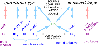
Figure 2: Lattice models of quantum and classical logics together with the corresponding equivalence relations which define their Lindenbaum-Tarski algebras.

The essence of the equivalence classes of the Lindenbaum-Tarski algebras is that they are determined by special simple lattices, e.g., those shown in Fig. 1, in which conditions that define particular other lattice models, fail. The failure is significant because it proves that the orthomodularity (30) of OML is not needed to prove the completeness of quantum logic for WOML2*, that neither the orthomodularity (30), nor condition (35) is needed to prove the completeness for WOML1*, and that neither the orthomodularity (30), nor condition (35), nor condition (34) is needed for WOML*.

With today’s computational technology we employ only bits and qubits which correspond to two-valued DL (digital, binary, two-valued Boolean algebra) and OML, respectively. This means that their possible valuations are reduced to {TRUE,FALSE} valuation for classical computation, i.e., when we implement classical logic, and to Hasse diagrams for quantum computation when we implement quantum logic McKay et al. (2000). So, it would be interesting to investigate how other valuations, i.e., various WOMLs and WDLs, can be implemented in complex circuits. That would provide us with the possibility of controlling essentially different algebraic structures (models) implemented into radically different hardware (logic circuits consisting of logic gates) by the same logic that we use today with the standard bit and qubit gate technology.

With these possible applications of quantum and classical logics we come back to the question which we started with: “Is Logic Empirical?” We have seen that logic is not uniquely empirical since it can simultaneously describe distinct realities. However, we have also seen (cf. Fig. 2) that by means of chosen relations of equivalence we can link particular kinds of “empirical” models to quantum logic on the one hand and to classical logic, on the other. Let us therefore briefly review the most recent elaborations on the question given by Bacciagaluppi Bacciagaluppi (2009) and Baltag and Smets Baltag and Smets (2011). They state: “Quantum logic is suitable as a logic that locally replaces classical logic when used to describe “a class of propositions in the context of quantum mechanical experiments”.”

Our results show that this point can be supported as follows. The propositions of quantum logic correspond to elements of a Hilbert lattice and are not directly linked to measurement values. Such logic employs models which evaluate particular combinations of propositions and tell us whether they are true or not. Evaluation means mapping from a set of propositions to lattice through which a correspondence with measurement values indirectly emerge. Since the strongest algebra (i.e., not O6, or WOML*, or WOML1*, or WOML2*, or …?) must be an orthomodular lattice but cannot be a Boolean algebra, we can say that quantum logic which has an orthomodular lattice as one of its models is “empirical” whenever we theoretically describe quantum measurements, simply because it can be linked to a model which serves for such a description: an orthomodular Hilbert lattice, i.e., the lattice of closed subspaces of a complex Hilbert space.

Conflicts of Interest

The author declares that there are no conflicts of interest regarding the publication of this paper.

References

- Putnam (1969) Hilary Putnam, “Is logic empirical,” in Boston Studies in the Philosophy of Science, Vol. V., Vol. V, edited by R. S. Cohen and M. W. Wartofsky (D. Reidel Publishing Company, Dordrecht, Holland, 1969) pp. 216–241.
- Birkhoff and von Neumann (1936) Garret Birkhoff and J. von Neumann, “The logic of quantum mechanics,” Ann. Math. 37, 823–843 (1936).
- Wilce (Fall 2012) Alexander Wilce, “Quantum logic and probability theory,” in The Stanford Encyclopedia of Philosophy, edited by Edward N. Zalta (Stanford University, Fall 2012) http://plato.stanford.edu/archives/fall2012/ entries/qt-quantlog/.
- Dishkant (1972) Hermann Dishkant, “Semantics of the minimal logic of quantum mechanics,” Studia Logica 30, 23–30 (1972).
- Goldblatt (1974) Robert I. Goldblatt, “Semantic analysis of orthologic,” J. Philos. Logic 3, 19–35 (1974).
- Dalla Chiara (1986) Maria Luisa Dalla Chiara, “Quantum logic,” in Handbook of Philosophical Logic, Vol. III., edited by D. Gabbay and F. Guenthner (D. Reidel, Dordrecht, 1986) pp. 427–469.
- Nishimura (1980) Hirokazu Nishimura, “Sequential method in quantum logic,” J. Symb. Logic 45, 339–352 (1980).
- Nishimura (2009) Hirokazu Nishimura, “Gentzen methods in quantum logic,” in Handbook of Quantum Logic and Quantum Structures, Vol. Quantum Logic, edited by Kurt Engesser, Dov Gabbay, and Daniel Lehmann (Elsevier, Amsterdam, 2009) pp. 227–260.
- Mittelstaedt (1978) Peter Mittelstaedt, Quantum Logic, Synthese Library; Vol. 126 (Reidel, London, 1978).
- Stachow (1976) Ernst-Walter Stachow, “Completeness of quantum logic,” J. Philos. Logic 5, 237–280 (1976).
- Pták and Pulmannová (1991) Pavel Pták and Sylvia Pulmannová, Orthomodular Structures as Quantum Logics (Kluwer, Dordrecht, 1991).
- Engesser and Gabbay (2002) Kurt Engesser and Dov M. Gabbay, Artificial Intelligence 136, 61–100 (2002).
- Rawling and Selesnick (2000) J. P. Rawling and S. A. Selesnick, “Orthologic and quantum logic: Models and computational elements,” JACM 47, 721–751 (2000).
- Herbut (2012) Fedor Herbut, “State-dependent implication and equivalence in quantum logic,” Adv. Math. Phys. 2012, 385341–1–23 (2012).
- Tylec and Kuś (2015) T. I. Tylec and M. Kuś, “Non-signaling boxes and quantum logics,” J. Phys. A 48, 505303–1–17 (2015).
- Bikchentaev et al. (2015) Airat Bikchentaev, Mirko Navara, and Rinat Yakushev, “Quantum logics of idempotents of unital rings,” Int. J. Theor. Phys. 54, 1987–2000 (2015).
- Engesser et al. (2007) Kurt Engesser, Dov M. Gabbay, and Daniel Lehmann, A New Approach to Quantum Logic (College Publications, 2007).
- Baltag and Smets (2005) Alexandru Baltag and Sonja Smets, “Complete axiomatizations of quantum actions,” Int. J. Theor. Phys. 44, 2267–2282 (2005).
- Baltag and Smets (2011) Alexandru Baltag and Sonja Smets, “Quantum logic as a dynamic logic,” Synthese 179, 285–306 (2011).
- Mateus and Sernadas (2006) P. Mateus and A. Sernadas, “Weakly complete axiomatization of exogenous quantum propositional logic,” Inform. Comput. 204, 771–794 (2006).
- Abramsky and Duncan (2006) Samson Abramsky and Ross Duncan, “A categorical quantum logic,” Math. Struct. Comp. Science 16, 469–489 (2006).
- Abramsky and Coecke (2004) Samson Abramsky and Bob Coecke, “A categorical semantics of quantum protocols,” in Proceedings of the 19th Annual IEEE Symposium on Logic in Computer Science: LICS 2004 (IEEE Computer Society, 2004) pp. 415––425.
- Harding (2009) John Harding, “A link between quantum logic and categorical quantum mechanics,” Int. J. Theor. Phys. 48, 769–802 (2009).
- Hilbert and Ackermann (1950) David Hilbert and Wilhelm Ackermann, Principles of Mathematical Logic (Chelsea, New York, 1950).
- Kalmbach (1983) Gudrun Kalmbach, Orthomodular Lattices (Academic Press, London, 1983).
- Kalmbach (1974) Gudrun Kalmbach, “Orthomodular logic,” Z. math. Logik Grundl. Math. 20, 395–406 (1974).
- Pavičić and Megill (1999) Mladen Pavičić and Norman D. Megill, “Non-orthomodular models for both standard quantum logic and standard classical logic: Repercussions for quantum computers,” Helv. Phys. Acta 72, 189–210 (1999).
- Pavičić and Megill (2009) Mladen Pavičić and Norman D. Megill, “Is quantum logic a logic?” in Handbook of Quantum Logic and Quantum Structures, Vol. Quantum Logic, edited by Kurt Engesser, Dov Gabbay, and Daniel Lehmann (Elsevier, Amsterdam, 2009) pp. 23–47.
- Pavičić and Megill (1998a) Mladen Pavičić and Norman D. Megill, “Binary orthologic with modus ponens is either orthomodular or distributive,” Helv. Phys. Acta 71, 610–628 (1998a).
- Schechter (2005) Eric Schechter, Classical and Nonclassical Logics: An Introduction to the Mathematics of Propositions (Princeton University Press, Princeton, 2005).
- Isham (1995) Chris J. Isham, Lectures on Quantum Theory (Imperial College Press, London, 1995).
- Halmos (1957) Paul R. Halmos, Introduction to Hilbert Space and the Spectral Theory of Spectral Multiplicity (Chelsea, New York, 1957).
- Holland, Jr. (1970) Samuel S. Holland, Jr., “The current interest in orthomodular lattices,” in Trends in Lattice Theory, edited by J. C. Abbot (Van Nostrand Reinhold, New York, 1970) pp. 41–126.
- Megill and Pavičić (2002) Norman D. Megill and Mladen Pavičić, “Deduction, ordering, and operations in quantum logic,” Found. Phys. 32, 357–378 (2002).
- Pavičić (1993) Mladen Pavičić, “Nonordered quantum logic and its YES-NO representation,” Int. J. Theor. Phys. 32, 1481–1505 (1993).
- Pavičić (1998) Mladen Pavičić, “Identity rule for classical and quantum theories,” Int. J. Theor. Phys. 37, 2099–2103 (1998).
- Note (1) The proof of the opposite claim in (Pavičić, 1993, Theorem 3.2) is wrong.
- Pavičić and Megill (2008) Mladen Pavičić and Norman D. Megill, “Standard logics are valuation-nonmonotonic,” J. Logic Comput. 18, 959–982 (2008).
- Beran (1985) Ladislav Beran, Orthomodular Lattices; Algebraic Approach (D. Reidel, Dordrecht, 1985).
- Megill and Pavičić (2003) Norman D. Megill and Mladen Pavičić, “Equivalencies, identities, symmetric differences, and congruencies in orthomodular lattices,” Int. J. Theor. Phys. 42, 2797–2805 (2003).
- McKay et al. (2000) Brendan D. McKay, Norman D. Megill, and Mladen Pavičić, “Algorithms for Greechie diagrams,” Int. J. Theor. Phys. 39, 2381–2406 (2000).
- Zeman (1978) J. Jay Zeman, “Generalized normal logic,” J. Philos. Logic 7, 225–243 (1978).
- Hardegree (1979) Gary M. Hardegree, “The conditional in abstract and concrete quantum logic,” in The Logico-Algebraic Approach to Quantum Mechanics, Vol. II. Contemporary Consolidation, edited by C. A. Hooker (D. Reidel, Dordrecht, 1979) pp. 49–108.
- Pavičić (1992) Mladen Pavičić, “Bibliography on quantum logics and related structures,” Int. J. Theor. Phys. 31, 373–461 (1992).
- Pavičić and Megill (1998b) Mladen Pavičić and Norman D. Megill, “Quantum and classical implication algebras with primitive implications,” Int. J. Theor. Phys. 37, 2091–2098 (1998b).
- Pavičić (1987) Mladen Pavičić, “Minimal quantum logic with merged implications,” Int. J. Theor. Phys. 26, 845–852 (1987).
- Pavičić (1989) Mladen Pavičić, “Unified quantum logic,” Found. Phys. 19, 999–1016 (1989).
- Bacciagaluppi (2009) Guido Bacciagaluppi, “Is logic empirical?” in Handbook of Quantum Logic and Quantum Structures, Vol. Quantum Logic, edited by Kurt Engesser, Dov Gabbay, and Daniel Lehmann (Elsevier, Amsterdam, 2009) pp. 49–78.