Stability of planar traveling waves
in a Keller-Segel equation
on an infinite strip domain

Abstract.

A simplified model of the tumor angiogenesis can be described by a Keller-Segel equation [8, 11, 20]. The stability of traveling waves for the one dimensional system has recently been known by [9, 14]. In this paper we consider the equation on the two dimensional domain $(x,y)\in\mathbb{R}\times{\mathbf{S}^{\lambda}}$ for a small parameter $\lambda>0$ where $\mathbf{S}^{\lambda}$ is the circle of perimeter $\lambda$. Then the equation allows a planar traveling wave solution of invading types. We establish the nonlinear stability of the traveling wave solution if the initial perturbation is sufficiently small in a weighted Sobolev space without a chemical diffusion. When the diffusion is present, we show a linear stability. Lastly, we prove that any solution with our front conditions eventually becomes planar under certain regularity conditions. The key ideas are to use the Cole-Hopf transformation and to apply the Poincaré inequality to handle with the two dimensional structure.

1. Introduction and main theorems

The formation of new blood vessels (angiogenesis) is the essential mechanism for tumour progression and metastasis. A simplified model of the tumor angiogenesis can be described by a Keller-Segel equation [8, 11, 20]. In this paper we consider the equation on the two dimensional cylindrical domain $(x,y)\in\Omega=\mathbb{R}\times[0,\lambda]$ with a front boundary condition in $x$ and the periodic condition in $y$, both specified later,

(1.1) $$\begin{aligned} \partial_{t}n-\Delta n&=-\nabla\cdot(n\chi(c)\nabla c),\\ \partial_{t}c-\epsilon\Delta c&=-c^{m}n\end{aligned}$$

with $m\geq 1$, where $n(x,y,t)\geq 0$ denote the density of endothelial cells, $c(x,y,t)\geq 0$ stands for the concentration of the chemical substance or the protein known as the vascular endothelial growth factor (VEGF) and $\chi(\cdot):\mathbb{R}^{+}\to\mathbb{R}^{+}$ is a decreasing chemosensitivity function, reflecting that the chemosensitivity is lower for higher concentration of the chemical. The system (1.1) includes the both zero chemical diffusion $(\epsilon=0)$ and non-zero chemical diffusion $(\epsilon>0)$ cases.
Endothelial cells forming the linings of the blood vessels are responsible for extending and remodeling the network of blood vessels, tissue growth and repair. Tumors or cancerous cells are also dependent on bloods supply by newly generated capillaries formed toward them, which process is called the endothelial angiogenesis. In the modeling the endothelial angiogenesis, the biological implication is that the endothelial cells behaves as a invasive species, responding to signals produced by the tissue. Accordingly the system (1.1) is given the front condition at left-right ends such that

(1.2) $$\lim_{x\to-\infty}n(x,y,t)=n_{-}>0,\quad\lim_{x\to\infty}n(x,y,t)=0,$$

(1.3) $$\lim_{x\to-\infty}c(x,y,t)=0,\quad\lim_{x\to\infty}c(x,y,t)=c_{+}>0.$$

We choose the $x$-axis by the propagating direction.

A planar traveling wave solution of (1.1) is a traveling wave solution independent of the transversal direction $y$ such that

(1.4) $$n(x,y,t)=N(x-st),\quad c(x,y,t)=C(x-st)$$

with a wave speed $s>0$. From now on, we consider only planar traveling waves $(N,C)$ satisfying the above boundary conditions (1.2) and (1.3), and moreover we assume

(1.5) $$N^{\prime}(\pm\infty)=C^{\prime}(\pm\infty)=0.$$

(We denote $\displaystyle\lim_{x\to\infty}N(x)$ by $N(\infty)$ in short.)
In this paper we study the stability of a planar traveling wave solution $(N,C)$ of (1.1) for $\epsilon\geq 0$ case assuming $\chi(c)=c^{-1}$, $m=1$,

(1.6) $$\begin{aligned} \partial_{t}n-\Delta n&=-\nabla\cdot\left(n\frac{\nabla c}{c}\right),\\ \partial_{t}c-\epsilon\Delta c&=-cn,\quad(x,y)\in\mathbb{R}\times[0,\lambda].\end{aligned}$$

We show that the planar traveling wave solution is asymptotically stable for certain small perturbations in a weighted Sobolev space when $\epsilon=0$ (Theorem 1.1), and linearly stable when $\epsilon>0$(Theorem 1.3). The restriction on $m=1$ is required for treating the singularity of $1/c$ by the Cole-Hopf transformation, as is presented in Section 2.2. On the other hand, the nonexistence of traveling wave solutions was proved in [21] when $m>1$.
The traveling wave solution with an invading front can be an evidence of the tumor encapsulation [1, 2, 22]. The existence of traveling wave solutions for a Keller-Segel model has been initiated by Keller and Segel [17] and was followed by many works. For instance, see [15] and the references therein. It is known that the chemosensitivity function $\chi(\cdot_{c})$ needs to be singular as $c$ approaches to zero for a traveling wave solution to exist ( e.g. see[17, 21]). The paper [17] and many others assume $\chi(c)=c^{-1}$ when studying traveling waves, which choice of $\chi(c)$ is also adopted when modeling the formation of the vascular network toward cancerous cells [8, 11, 20]. More general $\chi(c)$ other than $1/c$ together with the various production rates are studied in [16].

1.1. Main Theorems

Let us introduce the weight function:

$$w(x)=1+e^{sx},\quad x\in\mathbb{R}$$

and define the Sobolev spaces $H^{k}$ and $H^{k}_{w}$ by their norms:

$$\|\varphi\|_{H^{k}}^{2}=\sum_{i+j\leq k}\int_{\mathbb{R}\times[0,\lambda]}|\partial_{x}^{i}\partial_{y}^{j}\varphi(x,y)|^{2}dxdy,\quad$$

$$\|\varphi\|_{H^{k}_{w}}^{2}=\sum_{i+j\leq k}\int_{\mathbb{R}\times[0,\lambda]}|\partial_{x}^{i}\partial_{y}^{j}\varphi(x,y)|^{2}w(x)dxdy,\quad k=0,1,2\dots.$$

We will assume the periodic boundary condition in $y$-direction for initial perturbation and use the Sobolev spaces $H^{k}_{p}$ and $H^{k}_{w,p}$ :

$$H^{k}_{p} :={H^{k}}(\mathbb{R}\times\mathbf{S}^{\lambda})=\{\varphi\in{H^{k}}(\Omega)\,|\,\quad\sum_{i+j\leq k}\sum_{n\in\mathbb{Z}}\int_{\mathbb{R}}n^{2j}|\partial_{x}^{i}\varphi_{n}(x)|^{2}dx<\infty\},$$

$$H^{k}_{w,p} :={H^{k}_{w}}(\mathbb{R}\times\mathbf{S}^{\lambda})=\{\varphi\in{H^{k}_{w}}(\Omega)\,|\,\quad\sum_{i+j\leq k}\sum_{n\in\mathbb{Z}}\int_{\mathbb{R}}n^{2j}|\partial_{x}^{i}\varphi_{n}(x)|^{2}w(x)dx<\infty\}$$

where $\mathbf{S}^{\lambda}$ is the circle of perimeter $\lambda$ and $\varphi_{n}(x)$ is the $n$th Fourier coefficient of $\varphi(x,\cdot_{y})$.

In other words, $\varphi\in{H^{k}_{w,p}}$ is a function on $\mathbb{R}^{2}$ such that it is $\lambda$-periodic in $y$ and its (weighted in $z$-direction) $H^{k}$ norm on $\Omega=\mathbb{R}\times[0,\lambda]$ is finite. The cylindrical domain with this periodic boundary condition fits well to the picture that blood vessels are lined with a single layer of endothelial cells. What it follows we use the equivalence of $\|\cdot\|_{H^{k}_{p}}$ and $\|\cdot\|_{H^{k}_{w,p}}$ norms to $\|\cdot\|_{H^{k}}$ and $\|\cdot\|_{H^{k}_{w}}$ norms for functions periodic in $y$.
We perturb the system (1.6) around a planar traveling wave solution $(N,C)$ with the front conditions (1.2), (1.3) and (1.5) in a way that

(1.7) $$n(x,y,t) =N(x-st)+u(x-st,y,t)\quad\mbox{and }\quad c(x,y,t)=C(x-st)e^{-\psi(x-st,y,t)}$$

where the traveling wave speed $s=\sqrt{{\frac{n_{-}}{1+\epsilon}}}>0$. What it follows, we will use the moving frame

$$z=x-st.$$

We consider the above perturbation $(u,\psi)$ in the following function class.

1. There exists a vector-valued function $\varphi\in(H^{3}_{w,p})^{2}$ such that $u=\nabla\cdot\varphi=\partial_{z}\varphi^{1}+\partial_{y}\varphi^{2}$.

2. $\psi$ lies on $H^{3}_{p}$ with $\nabla\psi\in H^{2}_{w,p}$.

In the subsection 2.2, the nonlinear perturbation $(\varphi,\psi)$ is found directly related to the Cole-Hopf transformation.

We are ready to state the main results of the paper. The first result is on the nonlinear stability of the planar traveling wave solution $(N,C)$ of the system (1.6) when $\epsilon=0$.

Theorem 1.1.

For a given planar traveling wave solution $(N,C)$ of the system (1.6) for $\epsilon=0$ with (1.2), (1.3) and (1.5), there exist constants $m_{0}>0,\,C_{0}>0,$ and $\lambda_{0}>0$ such that if $0<\lambda\leq\lambda_{0}$, then for any initial data $(n_{0},c_{0})$ in the form of $N-n_{0}=\nabla\cdot\varphi_{0}$ and $c_{0}/C=e^{-\psi_{0}}$ where $\varphi_{0}$ and $\psi_{0}$ are $\lambda-$periodic in $y$ with $M_{0}:=\|\varphi_{0}\|^{2}_{H^{3}_{w}}+\|\psi_{0}\|^{2}_{H^{3}}+\|\nabla\psi_{0}\|^{2}_{H^{2}_{w}}\color[rgb]{0,0,0}\leq m_{0}$, there exist a unique global classical solution $(n,c)$ of (1.6) for $\epsilon=0$ in the form of

$$n(x,y,t)=N(x-st)+\nabla\cdot\varphi(x-st,y,t),\quad c(x,y,t)=C(x-st)e^{-\psi(x-st,y,t)},$$

where $\varphi$ and $\psi$ are $\lambda-$periodic in $y$ for each $t>0$ and $\varphi|_{t=0}=\varphi_{0}$ and $\psi|_{t=0}=\psi_{0}$. Moreover, $(\phi,\psi)$ satisfies the following inequality:

(1.8) $$\sup_{t\in[0,\infty)}\Big{(}\|\varphi\|^{2}_{H^{3}_{w}}+\|\psi\|^{2}_{H^{3}}+\|\nabla\psi\|^{2}_{H^{2}_{w}}\Big{)}+\int_{0}^{\infty}\Big{(}\|\nabla\varphi\|_{H^{3}_{w}}^{2}+\|\nabla\psi\|_{H^{2}_{w}}^{2}\Big{)}dt\leq C_{0}M_{0}.$$

Remark 1.2.

1. The condition $u=\nabla\cdot\varphi$ implies the zero integral condition on $u$, $\int udzdy=0$. Equivalently, $n$ and $N$ satisfy

   $$\int n(x,y,t)-N(x-st)dxdy=0,$$

   which is preserved over time, provided it holds at $t=0$ by the mass conservation property of $n$ equation.

2. The weight function $w$ is of a same order as $1/N$ in $z>0$ direction. More precisely, for a fixed traveling wave, there exists a constant $M$ satisfying

   $$\frac{w}{M}\leq\frac{1}{N}\leq Mw,$$

   which is proved in Section $2.4$.

3. Theorem 1.1 implies the asymptotic convergence of the primary perturbation of $(n,c)$ to $(N,C)$. From

   $$\int_{0}^{\infty}\Big{(}\|\nabla\varphi\|_{H^{3}_{w}}^{2}+\|\nabla\psi\|_{H^{2}_{w}}^{2}\Big{)}dt\leq C_{0}M_{0},$$

   we get a weak asymptotical estimate

   $$\liminf_{t\rightarrow\infty}\Big{(}\|\nabla\varphi(t)\|_{H^{3}_{w}}^{2}+\|\nabla\psi(t)\|_{H^{2}_{w}}^{2}\Big{)}=0.$$

   In terms of $n(\cdot_{z}+st)-N=\nabla\cdot\varphi$ and $c(\cdot_{z}+st)/C=e^{-\psi}$, we have

   $$\liminf_{t\rightarrow\infty}\Big{(}\|n(\cdot_{z}+st,\cdot_{y},t)-N(\cdot_{z})\|_{H^{3}_{w}}^{2}+\|\nabla\big{(}\log c(\cdot_{z}+st,\cdot_{y},t)-\log C(\cdot_{z})\big{)}\|_{H^{2}_{w}}^{2}\Big{)}=0.$$

4. The one-sided decay appears naturally with respect to the solvability of $\nabla\cdot\varphi=u$ in the infinite strip domain $\Omega$ [23]. Indeed, if there is a vector function $\varphi\in L^{2}(\Omega)$ satisfying the divergence equation, assuming Dirichlet or the periodic boundary condition on the lateral boundary, we have

   $$\int_{z>x}\int u(z,y)dzdy=\int_{z>x}\int_{[0,\lambda]}\nabla\cdot\varphi dzdy=-\int_{[0,\lambda]}\varphi^{1}(x,y)dy.$$

   Define $\mathcal{U}(x)=\int_{z>x}\int udydz$, then $\mathcal{U}(x)$ is found in $L^{2}([0,\infty))$ because

   $$\int_{0}^{\infty}\mathcal{U}^{2}(x)dx=\int_{0}^{\infty}\left(\int_{[0,\lambda]}\varphi^{1}(x,y)dy\right)^{2}dx\leq\int_{0}^{\infty}\lambda\int_{[0,\lambda]}|\varphi^{1}|^{2}(x,y)dydx=\lambda\|\varphi^{1}\|_{L^{2}}^{2}.$$

   In this paper, we do not pursuit solving $\nabla\cdot\varphi=u$ for a given perturbation $u$. Instead we are given $\varphi\in H^{3}_{w}$. Note that the condition $\|\varphi\|_{H^{3}_{w}}<\infty$ implies $wu\in L^{\infty}$, which is enough for $u$ to satisfy $\int_{0}^{\infty}\mathcal{U}^{2}dx<\infty$ and to be consistent with the necessary condtion for solvability. We refer to [23] for the solvability of the divergence equation on the more general noncompact domain.

When the chemical diffusion is present $(\epsilon>0)$, the above result of Theorem 1.1 is hard to obtain for technical reasons. Instead, we obtain a linear stability of the planar traveling wave solution $(N,C)$ of the system (1.6) when $\epsilon>0$ for perturbations in a smaller class(mean-zero in $y$). Indeed, as will be derived in Section 2.2, the pertubation $(\varphi,\psi)$ satisfies

(1.9) $$\begin{aligned} \varphi_{t}-s\varphi_{z}-\Delta\varphi&=N\nabla\psi+P\nabla\cdot\varphi+\nabla\cdot\varphi\nabla\psi,\\ \psi_{t}-s\psi_{z}-\epsilon\Delta\psi&=-2\epsilon P\cdot\nabla\psi-\epsilon|\nabla\psi|^{2}+\nabla\cdot\varphi\end{aligned}$$

where $P:=-(C^{\prime}/C,0)$. Quadratic terms dropped out, the linearized system of $(\varphi,\psi)$ is as follows:

(1.10) $$\begin{aligned} \varphi_{t}-s\varphi_{z}-\Delta\varphi&=N\nabla\psi+P\nabla\cdot\varphi,\\ \psi_{t}-s\psi_{z}-\epsilon\Delta\psi&=-2\epsilon P\cdot\nabla\psi+\nabla\cdot\varphi.\end{aligned}$$

What it follows we denote $\bar{\phi}(z)=\int_{0}^{\lambda}\phi(z,y)dy$.

Theorem 1.3.

For sufficiently small $\epsilon>0$ and for any given planar traveling wave solution $(N,C)$ of the system (1.6) with (1.2), (1.3) and (1.5), the wave $(N,C)$ is linearly stable in the following sense:
There exist constants $C_{0}>0,$ and $\lambda_{0}>0$ such that if $0<\lambda\leq\lambda_{0}$, then for any initial data $(\varphi_{0},\psi_{0})$ which is $\lambda-$periodic in $y$ with

$$\bar{\varphi}_{0}=\bar{\psi}_{0}=0\mbox{ and }M_{0}:=\|\varphi_{0}\|^{2}_{H^{3}_{w}}+\|\psi_{0}\|^{2}_{H^{3}}+\|\nabla\psi_{0}\|^{2}_{H^{2}_{w}}\color[rgb]{0,0,0}<\infty,$$

there exists a unique global classical solution $(\varphi,\psi)$ of (1.10) which is $\lambda-$periodic in $y$ and $\bar{\varphi}=\bar{\psi}=0$ for each $t>0$ and which satisfies the inequality:

(1.11) $$\sup_{t\in[0,\infty)}\Big{(}\|\varphi\|^{2}_{H^{3}_{w}}+\|\psi\|^{2}_{H^{3}}+\|\nabla\psi\|^{2}_{H^{2}_{w}}\Big{)}+\int_{0}^{\infty}\Big{(}\|\nabla\varphi\|_{H^{3}_{w}}^{2}+\|\nabla\psi\|_{H^{2}_{w}}^{2}{+\epsilon\|\nabla^{4}\psi\|_{H^{0}_{w}}^{2}}\Big{)}dt\leq C_{0}M_{0}.$$

The next theorem gives a hint why studying planar traveling waves is natural instead of studying general traveling waves in $\Omega$. Roughly speaking, any smooth bounded solution with our front boundary conditions (1.2), (1.3) becomes eventually planar under some strong regularity conditions when $\epsilon>0$. This kind of nonlinear stability can be found in [3] on the stability of a reactive Boussinesq system in an infinite vertical strip. It also hints the asymptotic stability as in Theorem 1.1 might hold as well in a nonzero diffusion case. We state this theorem in terms of $(n,q)$ in (2.5) which will be obtained in the subsection 2.2 by applying the Cole-Hopf transformation $q:=-\frac{\nabla c}{c}$ to (1.6).

Theorem 1.4.

Let $\epsilon>0$ and $(n,q)$ be a global smooth solution of (2.5) which is periodic in $y$ satisfying

$$\sup_{t\in[0,\infty)}\Big{(}\|n(t)\|_{L^{\infty}}+\|q(t)\|_{L^{\infty}}+\|\nabla q(t)\|_{L^{\infty}}\Big{)}<C_{1}$$

for some constant $C_{1}$. In addition, suppose that the derivatives of $(n,q)$ vanish sufficiently rapidly as $|x|\rightarrow\infty$. Then there exists a constant $c=c(\epsilon,\lambda)>0$ such that

$$\|n_{y}\|^{2}_{L^{2}}+\|q_{y}\|^{2}_{L^{2}}\leq(\|n_{y}(0)\|^{2}_{L^{2}}+\|q_{y}(0)\|^{2}_{L^{2}})e^{-ct}\quad\mbox{ for }t>0$$

if the transversal length $\lambda>0$ is sufficiently small.

Remark 1.5.

It implies $\lim_{t\rightarrow\infty}\Big{(}\|n_{y}\|_{L^{2}}+\|q_{y}\|_{L^{2}}\Big{)}=0.$

The remaining parts of the paper are organized as follows. In Section 2, we introduce the backgroud materials including the existence of traveling wave solutions and the Cole-Hopf trasformation. In Section 3, we prove Proposition 2.2 and 2.3, then establish Theorem 1.1. In Section 4, we prove the energy inequality (1.11) in Theorem 1.3. With (1.11) the existence part of Theorem 1.3 follows the same argument that works for the $\epsilon=0$ case, therefore we omitted. In the last section, we proves Theorem 1.4 which points out a nonlinear stability on a thin cylindrical domain for $\epsilon>0$ case would be expected as well.
There are many prior results on the existence of traveling wave solution and its stability. Among earlier analytic works is [19], where they proved the existence and linear instability of traveling wave solution of the one dimensional system when the bacterial consumption rate is constant and $\chi(c)=1/c$. The existence of the traveling wave solution with the front conditions (1.2) and (1.3) was shown in [26] when $\epsilon=0$, and [14, 25] when $\epsilon>0$. In the one dimensional system, the nonlinear asymptotic stability results were shown under the aforementioned restrictions on $\chi(c)$ and $m$ in [9] when $\epsilon=0$, and [14] when $\epsilon>0$ is small. To our knowledge, our Theorem 1.1 is the first result on a nonlinear stability of traveling wave solutions in a higher dimension.
For the results on the Cauchy problem of (1.1), see [4, 5, 7, 8, 12], where [4, 5] prove the existence of a global weak solution, and [12] proves that of a global classical solution. Both results consider the zero chemical diffusion case in a multi-dimension.

2. Background

2.1. Existence of traveling wave solutions

The traveling wave solution $(N,C)$ in (1.4) solves the following ODE system,

(2.1) $$\begin{aligned} -sN^{\prime}-N^{\prime\prime}=-(\chi(C)C^{\prime}N)^{\prime},\\ -sC^{\prime}-\epsilon C^{\prime\prime}=-C^{m}N.\end{aligned}$$

It is easy to see the above system integrable. We briefly discuss its solvability and properties of the solution for reader’s convenience. What it follows in this subsection has been already well known (for instance in [13, 25]).

Let $H^{\prime}(\cdot)=\chi(\cdot)$. We first solve $N$ by

$$N(z)=N_{0}e^{-sz}e^{H(C)}$$

for some positive constant $N_{0}$, which means a translation by $z_{0}$ when $N_{0}=e^{sz_{0}}$. The system (2.1) with the front conditions (1.2) and (1.3) is translation invariant. It causes the undetermined constant $N_{0}$.

To satisfy the front condition (1.2), we impose $e^{H(C)}\to 0$ as $z\to-\infty$, which implies $H(\cdot)$ is singular at zero such as $\lim_{C\to 0}H(C)=-\infty$. Substituting $N$ to the C equation, we have

$$sC^{\prime}+\epsilon C^{\prime\prime}=C^{m}e^{-sz}e^{H(C)}{N_{0}}.$$

What it follows we let

$$H(C)=\ln C,\quad m=1.$$

We result in

(2.2) $$N=e^{-sz}C{N_{0}},\quad sC^{\prime}+\epsilon C^{\prime\prime}=e^{-sz}C^{2}{N_{0}}.$$

By introducing

$$W=e^{-sz}C$$

we have a KPP-type equation for $W$:

(2.3) $$\epsilon W^{\prime\prime}+(s+2s\epsilon)W^{\prime}=-(\epsilon+1)s^{2}W+{N_{0}}W^{2}:=-f(W).$$

Since $N=WN_{0}$, front conditions (1.2), (1.3) force $W$ to have

$$\lim_{z\to-\infty}W(z)=\frac{1}{N_{0}}n_{-}\quad\lim_{z\to\infty}W(z)=0.$$

It is well known that the KPP- fisher equation (2.3) has a nonnegative solution if and only if $(s+2\epsilon s)\geq 2\sqrt{\epsilon(\epsilon+1)}s$, which automatically holds in this case. More precisely we refer to the following lemma in [25], which is based on the standard argument for the Fisher equation in [10, 18] etc.

Lemma 2.1.

[Wang, Lemma 3.2.] A nonnegative traveling wave solution $W$ of (2.3) exists. It satisfies $W^{\prime}<0,$

$$W_{-}=\frac{(1+\epsilon)s^{2}}{N_{0}},\mbox{ and }\quad W_{+}=0.$$

Moreover it is unique up to a translation in $x$, or $t$ and has the following asymptotic behavior:

$$W(x)-\frac{(\epsilon+1)s^{2}}{N_{0}}\sim Ce^{\lambda x}\mbox{ as }x\to-\infty\mbox{ and }\quad W(x)\sim(e^{-sx})\mbox{ as }x\to\infty$$

with $\lambda=\frac{-s(1+2\epsilon)+s\sqrt{(1+2\epsilon)^{2}+4\epsilon(1+\epsilon)}}{2\epsilon}$ when $\epsilon>0$ and $\lambda=-s$ when $\epsilon=0$.

To be consistent with Lemma 2.1, the wave speed $s$ is uniquely determined by $n_{-}$,

(2.4) $$s^{2}=\frac{n_{-}}{1+\epsilon}.$$

Also from $(C^{\prime}-sC)=e^{sz}W^{\prime}<0$ and the boundary condition $C(-\infty)=C^{\prime}(-\infty)=0$, we have

$$W^{\prime}(-\infty)=0.$$

We convert back $N$, $C$ satisfying (1.4) from $W$ with the required front condition (1.2), (1.3) and (1.5). The monotonicity of $N,C$ follows from $W^{\prime}<0$; the profile of $N$ is decreasing, and $C$ is increasing left to rightward.

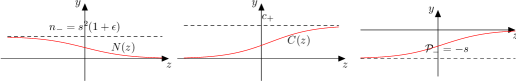
Figure 1. Monotonicity of $N$, $C$ and $\mathcal{P}$.

In the zero diffusion ($\epsilon=0$) we can explicitly solve (2.1)

$$sC^{\prime}=e^{-sz}C^{2}N_{0}$$

such that

$$C=\frac{c_{+}}{c_{+}\frac{N_{0}}{s^{2}}e^{-sz}+1}.$$

Then

$$N=\frac{c_{+}N_{0}e^{-sz}}{c_{+}\frac{N_{0}}{s^{2}}e^{-sz}+1}.$$

We have the relation $n_{-}=s^{2}$ and the monotone profile of $(N,C)$.

2.2. Cole-Hopf transformation

By the Cole-Hopf transformation

$$q=-\nabla\ln c=-\frac{\nabla c}{c}$$

We translate (1.6) into the divergence type equations of $(n,q)$

(2.5) $$\begin{aligned} \partial_{t}n-\Delta n&=\nabla\cdot(nq),\\ \partial_{t}q-\epsilon\Delta q&=-2\epsilon(q\cdot\nabla)q+\nabla n,\end{aligned}$$

with $((q\cdot\nabla)q)_{i}=\sum_{k=1,2}q_{k}\partial_{k}q_{i}$. This works only for $m=1$ in (1.1). The Cole-Hopf transformation is initiated in [14] for the stability problem of the traveling wave equation in the one-dimensional angiogenesis. It appears in [12] studying the multi-dimensional angiogenesis equation for $\epsilon=0$ with vanishing boundary conditions, too.
We shall add the condition

(2.6) $$\nabla\times q=\partial_{2}q_{1}-\partial_{1}q_{2}=0.$$

This curl free condition on $q$ is preserved in time until the classical local solution $(n,q)$ exists. It holds that

(2.7) $$q\cdot\nabla q=\frac{1}{2}\nabla|q|^{2}$$

with (2.6). We denote

(2.8) $$P=(\mathcal{P},0)=-(C^{\prime}/C,0)$$

then the perturbation (1.7) around $(N,C)$ is written by

(2.9) $$n(x,y,t)=N(x-st)+u(x-st,y,t),\quad q(x,y,t)=P(x-st)+\nabla\psi(x-st,y,t).$$

Note that $N,P(:=(\mathcal{P},0))$ solves

(2.10) $$\begin{aligned} -sN^{\prime}-N^{\prime\prime}&=(N\mathcal{P})^{\prime},\\ -s\mathcal{P}^{\prime}-\epsilon\mathcal{P}^{\prime\prime}&=-2\epsilon\mathcal{P}\mathcal{P}^{\prime}+N^{\prime}\end{aligned}$$

The boundary conditions of $(N,P)$ are inherited from those of $(N,C)$:

(2.11) $$\begin{aligned} &N(-\infty)=(1+\epsilon)s^{2},N(\infty)=0,\quad\mathcal{P}(-\infty)=-s,\mathcal{P}(\infty)=0,\\ &N^{\prime}(\pm\infty)=0,\quad P^{\prime}(\pm\infty)=0.\end{aligned}$$

For a while we denote

$$\nabla\psi=p.$$

So the curl-free condition is endowed to $p$. The perturbation $(u,p)$ satisfies

(2.12) $$\begin{aligned} &u_{t}-su_{z}-\Delta u=\nabla\cdot(Np+Pu+up),\\ &p_{t}-sp_{z}-\epsilon\Delta p=-2\epsilon\left(((P+p)\cdot\nabla)(P+p)-(P\cdot\nabla)P\right)+\nabla u.\end{aligned}$$

If we let

$$u=\nabla\cdot\varphi,\quad p=\nabla\psi,$$

the equation (2.12) is put into the equation on $(\varphi,\psi)$

(2.13) $$\begin{aligned} \varphi_{t}-s\varphi_{z}-\Delta\varphi&=N\nabla\psi+P\nabla\cdot\varphi+\nabla\cdot\varphi\nabla\psi,\\ \psi_{t}-s\psi_{z}-\epsilon\Delta\psi&=-2\epsilon P\cdot\nabla\psi-\epsilon|\nabla\psi|^{2}+\nabla\cdot\varphi.\end{aligned}$$

2.3. Main proposition for Theorem 1.1

From now on, we fix a planar traveling wave solution $(N,C)$ of the system (1.6) for $\epsilon=0$ with (1.2), (1.3) and (1.5), obtained in Section 2.1. The pertubation $(\varphi,\psi)$ satisfies the system

(2.14) $$\begin{aligned} \varphi_{t}-s\varphi_{z}-\Delta\varphi&=N\nabla\psi+P\nabla\cdot\varphi+\nabla\cdot\varphi\nabla\psi,\\ \psi_{t}-s\psi_{z}&=\nabla\cdot\varphi\end{aligned}$$

for $(t,z,y)\in[0,\infty)\times\mathbb{R}\times[0,\lambda]$ where $P=-(C^{\prime}/C,0)$ as in (2.8). In addition, recall the function spaces and the periodic condition (in $y$-direction) for $(\varphi,\psi)$ which are discussed prior to the main Theorem 1.1.

First we state a result on the local existence of solutions for the system (2.14) which can be proved in the standard manner. The proof is presented at the end of the section 3 (Subsection 3.3).

Proposition 2.2.

For $\lambda>0$ and $M>0$, there exists $T_{0}>0$ such that for any initial data $(\varphi_{0},\psi_{0})$ which is $\lambda-$periodic in $y$ with $\|\varphi_{0}\|^{2}_{H^{3}_{w}}+\|\psi_{0}\|^{2}_{H^{3}}+\|\nabla\psi_{0}\|^{2}_{H^{2}_{w}}<M$, the system (2.14) has a unique solution $(\varphi,\psi)$ on $[0,T_{0}]$ which is $\lambda-$periodic in $y$ for each $t\in[0,T_{0}]$ with $\varphi|_{t=0}=\varphi_{0}$ and $\psi|_{t=0}=\psi_{0}$ and

$$\varphi\in L^{\infty}(0,T_{0};H^{3}_{w}),\quad\psi\in L^{\infty}(0,T_{0};H^{3}),\quad\nabla\psi\in L^{\infty}(0,T_{0};H^{2}_{w})\color[rgb]{0,0,0}.$$

Moreover it holds the following inequality:

(2.15) $$\sup_{t\in[0,T_{0}]}\Big{(}\|\varphi\|^{2}_{H^{3}_{w}}+\|\psi\|^{2}_{H^{3}}+\|\nabla\psi\|^{2}_{H^{2}_{w}}\Big{)}\leq 2M.$$

Let us state the result on the existence of global classical solution to the system (2.14). Due to our derivation of (2.14) from (1.6), the main Theorem 1.1 is the direct consequence of Proposition 2.3, which will be proved in Section $3$.

Proposition 2.3.

There exist constants $m_{0}>0,\,C_{0}>0$, and $\lambda_{0}>0$ such that for $0<\lambda\leq\lambda_{0}$ and for any initial data $(\varphi_{0},\psi_{0})$ which is $\lambda-$periodic in $y$ with $M_{0}:=\|\varphi_{0}\|^{2}_{H^{3}_{w}}+\|\psi_{0}\|^{2}_{H^{3}}+\|\nabla\psi_{0}\|^{2}_{H^{2}_{w}}\color[rgb]{0,0,0}\leq m_{0}$, there exists a unique global classical solution $(\varphi,\psi)$ of (2.14) which is $\lambda-$periodic in $y$ for each $t>0$ with $\varphi|_{t=0}=\varphi_{0}$ and $\psi|_{t=0}=\psi_{0}$. Moreover, $(\phi,\psi)$ satisfies the inequality

$$\sup_{t\in[0,\infty)}\Big{(}\|\varphi\|^{2}_{H^{3}_{w}}+\|\psi\|^{2}_{H^{3}}+\|\nabla\psi\|^{2}_{H^{2}_{w}}\Big{)}+\int_{0}^{\infty}\Big{(}\|\nabla\varphi\|_{H^{3}_{w}}^{2}+\|\nabla\psi\|_{H^{2}_{w}}^{2}\Big{)}dt\leq C_{0}M_{0}.$$

In the below we summarize the notations used in the paper.

$$w(z):=1+e^{sz},$$

$$M(t):=\sup_{s\in[0,t]}(\|\varphi(s)\|^{2}_{H^{3}_{w}}+\|\psi(s)\|^{2}_{H^{3}}+\|\nabla\psi(s)\|^{2}_{H^{2}_{w}}),$$

$$M_{0}:=(\|\varphi_{0}\|^{2}_{H^{3}_{w}}+\|\psi_{0}\|^{2}_{H^{3}}+\|\nabla\psi_{0}\|^{2}_{H^{2}_{w}}),$$

$$\|f\|:=\|f\|_{L^{2}(\Omega)},$$

$$\|f\|^{2}_{k}:=\|f\|^{2}_{H^{k}}=\sum_{|\alpha|=0}^{k}\int_{\Omega}|D^{\alpha}f|^{2}\,dzdy,$$

$$\|f\|^{2}_{k,w}:=\|f\|^{2}_{H^{k}_{w}}=\sum_{|\alpha|=0}^{k}\int_{\Omega}|D^{\alpha}f(z,y)|^{2}\,w(z)dzdy,$$

$$\int f:=\int_{\Omega}f(z,y)dzdy,$$

$$\int_{0}^{t}g:=\int_{0}^{t}g(s)ds.$$

3. Uniform in time estimate when $\epsilon=0$

In this section we introduce the main proposition 3.1 below which implies Proposition 2.3.

Proposition 3.1.

There exist constants $\delta_{0}>0,\,C_{0}$, and $\lambda_{0}>0$ such that for $\lambda\in(0,\lambda_{0}]$, we have the following:
If $(\varphi,\psi)$ be a local solution of (2.14) on $[0,T]$ for some $T>0$ with

$$M(T)\leq\delta\quad\mbox{(the bootstrap assumption)}$$

for some initial data $(\varphi_{0},\psi_{0})$ which is $\lambda$-periodic in $y$, then we have

(3.1) $$M(T)+\int_{0}^{T}\sum_{l=1}^{4}\|\nabla^{l}\varphi\|_{w}^{2}+\int_{0}^{T}\sum_{l=1}^{3}\|\nabla^{l}\psi\|_{w}^{2}\leq C_{0}M_{0}.$$

This proposition will be proved in Subsection 3.2.

Remark 3.2.

Note that the constant $C_{0}$ in the above proposition does not depend on the size of $T>0$. This fact immediately improves the bootstrap assumption if we take a sufficiently small initial data, for instance, satisfying $C_{0}M_{0}<\delta_{0}/2$. Once we prove the proposition, then the global-existence statement in Proposition 2.3 follows the standard continuation argument as shown below:

Proof of Proposition 2.3 from Proposition 3.1.

Let $M:=\delta_{0}/2,\,m_{0}:=M/C_{0}$ where $\delta_{0}$ and $C_{0}$ are the constants in Proposition 3.1. We may assume $C_{0}\geq 1$. Consider the initial data $(\varphi_{0},\psi_{0})$ with $M(0)=M_{0}\leq m_{0}\leq M$. By using this constant $M$ to the local-existence result (Proposition 2.2), there exist $T_{0}>0$ and the unique local solution $(\varphi,\psi)$ on $[0,T_{0}]$ with $M(T_{0})\leq 2M$. Due to $M(T_{0})\leq 2M\leq\delta_{0}$, we can use the result of Proposition 3.1 to obtain $M(T_{0})\leq C_{0}M_{0}$, which implies $M(T_{0})\leq C_{0}m_{0}\leq M$. Hence we can extend the solution up to the time $2T_{0}$ by Proposition 2.2 and we obtain $M(2T_{0})\leq 2M\leq\delta_{0}$. Due to Proposition 3.1, it implies $M(2T_{0})\leq C_{0}M_{0}\leq M$. Thus we can repeat this process of extension to get $M(kT_{0})\leq C_{0}M_{0}$ for any $k\in\mathbb{N}$. ∎

First we summarize some properties of traveling waves $(N,\mathcal{P})$ for later analysis.

3.1. Properties on $(N,\mathcal{P})$

From the equations:

(3.2) $$\begin{aligned} -sN^{\prime}-N^{\prime\prime}&=(N\mathcal{P})^{\prime},\\ -s\mathcal{P}^{\prime}&=N^{\prime},\end{aligned}$$

we observe the relations

(3.3) $$\frac{\mathcal{P}}{N}=-\frac{1}{s}\quad\mbox{and }\left(\frac{1}{N}\right)^{{}^{\prime\prime}}=s\left(\frac{1}{N}\right)^{{}^{\prime}}$$

from (3.4) where $s>0$, which is fixed throughout this paper, is the speed of our planar traveling wave $(N,C)$. In fact, $(N,P)$ has the explicit formula:

(3.4) $$N=\frac{c_{+}N_{0}e^{-sz}}{c_{+}\frac{N_{0}}{s^{2}}e^{-sz}+1},\quad P=-\left(\frac{c_{+}N_{0}e^{-sz}}{c_{+}\frac{N_{0}}{s}e^{-sz}+s},0\right).$$

Note that $N$ and $\mathcal{P}$ are monotone with the boundary condition (2.11).

In the following lemma, we summarize some properties of $(N,\mathcal{P})$.

Lemma 3.3.

There exists a constant $M>0$ such that we have:

$$\frac{w}{M}\leq\frac{1}{N}\leq Mw,$$

$$|{N^{(k)}}|\leq M,\quad|{\mathcal{P}^{(k)}}|\leq M,\quad\mbox{ for }0\leq k\leq 2,\quad\mbox{ and }$$

$$\frac{N^{\prime}}{N}=-(\mathcal{P}+s),\quad\Big{|}(\frac{1}{N})^{\prime}\Big{|}+\Big{|}(\frac{1}{N})^{\prime\prime}\Big{|}\leq\frac{M}{N},\quad\Big{|}(\frac{1}{\sqrt{N}})^{\prime}\Big{|}\leq\frac{M}{\sqrt{N}}.$$

($N^{(k)}$ is any $k-$th derivative of $N$)

Proof.

The first inequality follows from Lemma 2.1. The others are easily obtained from the equation (3.2) and (3.3). ∎

3.2. Proof of Proposition 3.1

First assume $0<\delta_{0}\leq 1$. During the proof, we will take $\delta_{0}$ as small as needed to have the weighted energy estimate (3.1) (e.g. Lemma 3.10). Let us remind the system (2.14)

(3.5) $$\begin{aligned} \varphi_{t}-s\varphi_{z}-\Delta\varphi&=N\nabla\psi+P\nabla\cdot\varphi+\nabla\cdot\varphi\nabla\psi,\\ \psi_{t}-s\psi_{z}&=\nabla\cdot\varphi\\ \end{aligned}$$

for $(t,z,y)\in[0,T]\times\mathbb{R}\times[0,\lambda]$. We will collect a few lemmas on energy estimates before proving Proposition 3.1. Here the constants $C$ which will appear in the following lemmas are independent of $T>0$.

Lemma 3.4.

If $\lambda>0$ is sufficiently small, we have the following:

(3.6) $$\|\psi\|^{2}+\|\varphi\|_{w}^{2}+\int_{0}^{t}\|\nabla\varphi\|_{w}^{2}\leq C(\|\psi_{0}\|^{2}+\|\varphi_{0}\|_{w}^{2})+C{{M(t)}}\int_{0}^{t}\|\nabla\psi\|_{w}^{2}.$$

Remark 3.5.

This estimate (3.6) is not closed due to the second term in the right-hand side. This obstacle will be studied sequentially in the next lemmas.

Proof.

Multiply $\frac{\varphi}{N}$ to the $\varphi$ equation and $\psi$ to the $\psi$ equation. Integrating by parts, we have

$$\frac{1}{2}\frac{d}{dt}\left(\int\frac{|\varphi|^{2}}{N}+\int|\psi|^{2}\right)+\int\frac{\sum_{i}|\nabla\varphi^{i}|^{2}}{N}+\frac{s}{2}\int|\varphi|^{2}\left(\frac{1}{N}\right)^{\prime}$$

$$=\frac{1}{2}\int|\varphi|^{2}\left(\frac{1}{N}\right)^{\prime\prime}+\int\frac{\mathcal{P}}{N}\varphi^{1}\nabla\cdot\varphi+\int\frac{\varphi\cdot\nabla\psi}{N}\nabla\cdot\varphi.$$

We estimate the cubic term first:

$$\int\frac{\varphi\cdot\nabla\psi}{N}\nabla\cdot\varphi \leq{C\int\frac{\|\varphi\|_{L^{\infty}}^{2}|\nabla\psi|^{2}}{N}+\frac{1}{4}\int\frac{|\nabla\varphi|^{2}}{N}\leq C{M(t)}\int\frac{|\nabla\psi|^{2}}{N}+\frac{1}{4}\int\frac{|\nabla\varphi|^{2}}{N}}$$

where we used $\|\varphi\|_{L^{\infty}}\leq C\|\varphi\|_{H^{2}}\leq C\sqrt{M(t)}$ by the Sobolev embedding.

Thanks to the relations (3.3), the quadratic term becomes

(3.7) $$\int\frac{\mathcal{P}}{N}\varphi^{1}\nabla\cdot\varphi =-\frac{1}{s}\int\varphi^{1}(\partial_{z}\varphi^{1}+\partial_{y}\varphi^{2})=-\frac{1}{s}\int(\varphi^{1}-\overline{\varphi}^{1})\partial_{y}\varphi^{2}$$

where $\overline{\varphi}(z)=(1/\lambda)\int_{[0,\lambda]}\varphi(z,y)dy$ is the average in $y$ of $\varphi$ for each $z$. Note that we used the periodic condition for $\varphi^{2}$. As a result, we get

$$\Big{|}\int\frac{\mathcal{P}}{N}\varphi^{1}\nabla\cdot\varphi\Big{|} \leq C\frac{\lambda}{s}\|\partial_{y}\varphi^{1}\|_{2}\|\partial_{y}\varphi^{2}\|_{2}\leq C\lambda\|\nabla\varphi\|^{2}_{w}$$

where we used the Poincaré inequality

(3.8) $$\|\varphi(z,\cdot_{y})-\overline{\varphi}(z)\|_{L^{2}_{y}([0,\lambda])}\leq C\lambda\|\partial_{y}\varphi(z,\cdot_{y})\|_{L^{2}_{y}([0,\lambda])}\quad\mbox{ for }z\in\mathbb{R}.$$

Also we have

$${\frac{s}{2}\int|\varphi|^{2}\left(\frac{1}{N}\right)^{\prime}-\frac{1}{2}\int|\varphi|^{2}\left(\frac{1}{N}\right)^{\prime\prime}}{=0}$$

thanks to the relations (3.3). By assuming smallness of $\lambda$, we get the following:

$$\frac{1}{2}\frac{d}{dt}\left(\int\frac{|\varphi|^{2}}{N}+\int|\psi|^{2}\right)+\frac{1}{8}\int\frac{|\nabla\varphi|^{2}}{N}\leq C{{M(t)}}\int\frac{|\nabla\psi|^{2}}{N}.$$

It proves Lemma 3.4.

∎

Let’s study the first order estimate:

Lemma 3.6.

If $\lambda>0$ is small enough, then we have

(3.9) $$\begin{split}&\|\nabla\varphi\|_{w}^{2}+\|\nabla\psi\|^{2}+\int_{0}^{t}\|\nabla^{2}\varphi\|_{w}^{2}\\ &\leq C(\|\nabla\varphi_{0}\|_{w}^{2}+\|\nabla\psi_{0}\|^{2}+\|\psi_{0}\|^{2}+\|\varphi_{0}\|_{w}^{2})+C\int_{0}^{t}\int{N}|\nabla\psi|^{2}+C{{M(t)}}\int_{0}^{t}\int\frac{|\nabla\psi|^{2}}{N}.\end{split}$$

Remark 3.7.

This estimate (LABEL:ineq:lem1_) is not closed yet due to the last two terms. Later in Lemma 3.11 (see the estimate (3.17)), it will be closed by Lemma 3.8 and Lemma 3.10. Indeed, the first one $\int_{0}^{t}\int{N}|\nabla\psi|^{2}$ among these two will be covered by the second one $\sqrt{M(t)}\int_{0}^{t}\int\frac{|\nabla\psi|^{2}}{N}$ (see Lemma 3.8) while the second term will be absorbed into the dissipation term $\int_{0}^{t}\|\nabla^{2}\varphi\|_{w}^{2}$ on the left-hand side of (LABEL:ineq:lem1_) (see Lemma 3.10).

Proof.

Differentiating in $z$, we have

$$\varphi_{tz}-s\varphi_{zz}-\Delta\varphi_{z} =N^{\prime}\nabla\psi+N\nabla\psi_{z}+P^{\prime}\nabla\cdot\varphi+P\nabla\cdot\varphi_{z}+\nabla\psi_{z}\nabla\cdot\varphi+\nabla\psi\nabla\cdot\varphi_{z},$$

$$\psi_{tz}-s\psi_{zz} =\nabla\cdot\varphi_{z}.$$

Multiply $\frac{\varphi_{z}}{N}$ and $\psi_{z}$ to the above equation. Integrating by parts, we have

$$\frac{1}{2}\frac{d}{dt}\left(\int\frac{|\varphi_{z}|^{2}}{N}+|\psi_{z}|^{2}\right)+\int\sum_{ij}\frac{|\partial_{j}\varphi^{i}_{z}|^{2}}{N} ={\frac{1}{2}\int|\varphi_{z}|^{2}\left(\frac{1}{N}\right)^{\prime\prime}-\frac{s}{2}\int|\varphi_{z}|^{2}\left(\frac{1}{N}\right)^{\prime}}$$

$$+\int\frac{N^{\prime}}{N}\nabla\psi\varphi_{z}+\int\frac{P^{\prime}}{N}\nabla\cdot\varphi\varphi_{z}+\int\frac{P}{N}\nabla\cdot\varphi_{z}\varphi_{z}$$

$$+\int\nabla\psi_{z}\nabla\cdot\varphi\frac{\varphi_{z}}{N}+\int\nabla\psi\nabla\cdot\varphi_{z}\frac{\varphi_{z}}{N}.$$

Similarly, we get

$$\frac{1}{2}\frac{d}{dt}\left(\int\frac{|\varphi_{y}|^{2}}{N}+|\psi_{y}|^{2}\right)+\int\sum_{ij}\frac{|\partial_{j}\varphi^{i}_{y}|^{2}}{N} ={\frac{1}{2}\int|\varphi_{y}|^{2}\left(\frac{1}{N}\right)^{\prime\prime}-\frac{s}{2}\int|\varphi_{y}|^{2}\left(\frac{1}{N}\right)^{\prime}}$$

$$+\int\frac{P}{N}\nabla\cdot\varphi_{y}\varphi_{y}$$

$$+\int\nabla\psi_{y}\nabla\cdot\varphi\frac{\varphi_{y}}{N}+\int\nabla\psi\nabla\cdot\varphi_{y}\frac{\varphi_{y}}{N}.$$

First, we estimate by using Lemma 3.3

$$\frac{1}{2}\int|\nabla\varphi|^{2}\left(\frac{1}{N}\right)^{\prime\prime}-\frac{s}{2}\int|\nabla\varphi|^{2}\left(\frac{1}{N}\right)^{\prime}\leq-\int\nabla\varphi\cdot\nabla\varphi_{z}\left(\frac{1}{N}\right)^{\prime}+\frac{s}{2}\int|\nabla\varphi|^{2}\left|\left(\frac{1}{N}\right)^{\prime}\right|$$

$$\leq C\int|\nabla\varphi||\nabla\varphi_{z}|\left(\frac{1}{N}\right)+\frac{Cs}{2}\int|\nabla\varphi|^{2}\left(\frac{1}{N}\right)\leq\frac{1}{4}\int|\nabla\varphi_{z}|^{2}\left(\frac{1}{N}\right)+(C+\frac{Cs}{2})\int|\nabla\varphi|^{2}\left(\frac{1}{N}\right).$$

We estimate the quadratic terms as follows:

$$\int\frac{P}{N}\nabla\cdot\varphi_{z}\varphi_{z}+\int\frac{P}{N}\nabla\cdot\varphi_{y}\varphi_{y}\leq\|P\|_{L^{\infty}}(\|\frac{\nabla\varphi_{z}}{\sqrt{N}}\|\|\frac{\varphi_{z}}{\sqrt{N}}\|+\|\frac{\nabla\varphi_{y}}{\sqrt{N}}\|\|\frac{\varphi_{y}}{\sqrt{N}}\|)\leq\frac{1}{4}\|\frac{\nabla^{2}\varphi}{\sqrt{N}}\|^{2}+C\|\frac{\nabla\varphi}{\sqrt{N}}\|^{2},$$

$$\int\frac{N^{\prime}}{N}\nabla\psi\varphi_{z} \leq\|\frac{N^{\prime}}{N}\|_{L^{\infty}}\|{\sqrt{N}}{\nabla\psi}\|\|\frac{\varphi_{z}}{\sqrt{N}}\|\leq C\|{\sqrt{N}}{\nabla\psi}\|^{2}+C\|\frac{\nabla\varphi}{\sqrt{N}}\|^{2},$$

$$\int\frac{P^{\prime}}{N}\nabla\cdot\varphi\varphi_{z} \leq\|P^{\prime}\|_{L^{\infty}}\|\frac{\nabla\varphi}{\sqrt{N}}\|^{2}\leq C\|\frac{\nabla\varphi}{\sqrt{N}}\|^{2}.$$

The cubic terms are bounded by

$$\int|\nabla\psi||\nabla\varphi|\frac{|\nabla^{2}\varphi|}{N}+\int|\nabla\psi||\nabla\varphi|^{2}\underbrace{|({1}/{N})^{\prime}|}_{\leq C/{N}} {\leq\frac{1}{4}\|\nabla^{2}\varphi/\sqrt{N}\|^{2}+C(M(t)+\sqrt{M(t)})\|\nabla\varphi/\sqrt{N}\|^{2}}$$

$${\leq\frac{1}{4}\|\nabla^{2}\varphi/\sqrt{N}\|^{2}+C\|\nabla\varphi/\sqrt{N}\|^{2}}$$

by $\|\nabla\psi\|_{L^{\infty}}\leq C\sqrt{M(t)}$ and by the assumption $M(t)\leq M(T)\leq 1$.

Adding up all the estimates above, we have

$$\frac{1}{2}\frac{d}{dt}\left(\int\frac{|\nabla\varphi|^{2}}{N}+\int|\nabla\psi|^{2}\right)+\frac{1}{4}\int\frac{|\nabla^{2}\varphi|^{2}}{N}\leq C\|{\sqrt{N}}{\nabla\psi}\|^{2}+C\|\frac{\nabla\varphi}{\sqrt{N}}\|^{2}.$$

After integration in time, thanks to Lemma 3.4, we can control the last term above so that we arrive at (LABEL:ineq:lem1_). ∎

Lemma 3.8.

If $\lambda>0$ is small enough, then we have

(3.10) $$\int_{0}^{t}\int N|\nabla\psi|^{2}\leq C\left(\|\nabla\psi_{0}\|^{2}+\|\psi_{0}\|^{2}+\|\varphi_{0}\|_{w}^{2}\right)+C\sqrt{M(t)}\int_{0}^{t}\int\frac{|\nabla\psi|^{2}}{N}.$$

Remark 3.9.

1. Roughly speaking, this estimate moves $N(z)$ to the denominator, while the integral multiplied by $\sqrt{M(t)}$ which can be assumed small enough.

2. This estimate for $\int_{0}^{t}\int N|\nabla\psi|^{2}$ is due to the special structure (2.14). Note that the $\varphi$-equation has the term $N\nabla\psi$ on its right hand.

Proof.

Multiplying $\nabla\psi$ to the $\varphi$-equation, we have

(3.11) $$N|\nabla\psi|^{2}=\underbrace{\varphi_{t}\cdot\nabla\psi}_{(A)}-s\varphi_{z}\cdot\nabla\psi-\underbrace{\Delta\varphi\cdot\nabla\psi}_{(B)}-(\nabla\cdot\varphi)P\cdot\nabla\psi-\nabla\cdot\varphi|\nabla\psi|^{2}.$$

Let us rewrite the terms $(A)$ and $(B)$.

$$(A) =(\varphi\cdot\nabla\psi)_{t}-\varphi\cdot\nabla\psi_{t}$$

$$=(\varphi\cdot\nabla\psi)_{t}-\varphi\cdot(s\nabla\psi_{z}+\nabla(\nabla\cdot\varphi)$$

and

$$(B)=(\nabla\cdot\varphi)_{z}\psi_{z}+(\varphi^{1}_{yy}-\varphi^{2}_{zy})\psi_{z}+(\nabla\cdot\varphi)_{y}\psi_{y}+(\varphi^{2}_{zz}-\varphi^{1}_{zy})\psi_{y}.$$

Integration by parts gives

$$\int(B)=\int(\nabla\cdot\varphi)_{z}\psi_{z}+(\nabla\cdot\varphi)_{y}\psi_{y}=\int\nabla(\nabla\cdot\varphi)\cdot\nabla\psi.$$

By using the $\psi$-equation which has $\nabla\cdot\varphi$ on its right side, we get

$$\int\nabla(\nabla\cdot\varphi)\cdot\nabla\psi =\int\nabla(\psi_{t}-s\psi_{z})\cdot\nabla\psi=\frac{1}{2}\frac{d}{dt}\int|\nabla\psi|^{2}.$$

Integration on (3.11) gives us

$$\int N|\nabla\psi|^{2}= \frac{d}{dt}\int\varphi\cdot\nabla\psi-\int s\varphi\cdot\nabla\psi_{z}-\int\varphi\cdot(\nabla(\nabla\cdot\varphi))$$

$$-\int s\varphi_{z}\cdot\nabla\psi$$

$$-\frac{1}{2}\frac{d}{dt}\int(\psi_{z}^{2}+\psi_{y}^{2})$$

$$-\int(\nabla\cdot\varphi)P\cdot\nabla\psi-\int\nabla\cdot\varphi|\nabla\psi|^{2}.$$

We rearrange the above to get

(3.12) $$\int N|\nabla\psi|^{2}= \frac{d}{dt}\int\varphi\cdot\nabla\psi-\frac{1}{2}\frac{d}{dt}\int|\nabla\psi|^{2}$$

$$+\int|\nabla\cdot\varphi|^{2}-\int(\nabla\cdot\varphi)P\cdot\nabla\psi-\int\nabla\cdot\varphi|\nabla\psi|^{2}$$

$$=(I)+(II).$$

Note that

$${\int_{0}^{t}(I)}=\int_{0}^{t}\left(\frac{d}{dt}\int\varphi\cdot\nabla\psi-\frac{1}{2}\frac{d}{dt}\int|\nabla\psi|^{2}\right)\leq{C(\|\varphi(t)\|^{2}+\|\nabla\psi_{0}\|^{2}+\|\varphi_{0}\|^{2})}$$

by $\int\varphi\nabla\psi\leq C\|\varphi\|^{2}+\frac{1}{2}\|\nabla\psi\|^{2}$.

For the second term $(II)$, we estimate

$$\int|\nabla\cdot\varphi|^{2}-\int(\nabla\cdot\varphi)P\cdot\nabla\psi \leq C\int\frac{|\nabla\varphi|^{2}}{N}+\frac{1}{4}\int N|\nabla\psi|^{2},$$

$$\int|\nabla\cdot\varphi||\nabla\psi|^{2} \leq C\sqrt{M(t)}\int{|\nabla\psi|^{2}}\leq C\sqrt{M(t)}\int\frac{|\nabla\psi|^{2}}{N}$$

by bounding $\|\nabla\cdot\varphi\|_{L^{\infty}}\leq C\|\nabla\cdot\varphi\|_{H^{2}}\leq C\sqrt{M(t)}$.

Now integrating (3.12) in time, we get

$$\int_{0}^{t}\int N|\nabla\psi|^{2}\leq C(\|\varphi(t)\|^{2}+\|\nabla\psi_{0}\|^{2}+\|\varphi_{0}\|^{2})$$

$$+\int_{0}^{t}\Big{(}C\|\nabla\varphi\|_{w}^{2}+\frac{1}{4}\int N|\nabla\psi|^{2}+C\sqrt{M(t)}\int\frac{|\nabla\psi|^{2}}{N}\Big{)}.$$

By Lemma 3.4 and by $M(t)\leq\sqrt{M(t)}$, we have (3.10). ∎

What remains to close (LABEL:ineq:lem1_) is to control the term $\sqrt{M(t)}\int_{0}^{t}\int\frac{|\nabla\psi|^{2}}{N}$. Note that $\psi$-equation lacks diffusion of closing the estimates without weight. However, our choice of the one-sided exponential weight function $w(\cdot)$ gives a one-sided dissipation $\int_{0}^{t}\int_{z>0}\frac{|\nabla\psi|^{2}}{N}$ as shown below.

Lemma 3.10.

If $M(T)>0$ and $\lambda>0$ are small enough, then we have

(3.13) $$\int\frac{|\nabla\psi|^{2}}{N}+\int_{0}^{t}\int\frac{|\nabla\psi|^{2}}{N}\leq C(\|\nabla\psi_{0}\|_{w}^{2}+\|\psi_{0}\|^{2}+\|\varphi_{0}\|_{w}^{2})+C\int_{0}^{t}\int\frac{|\nabla^{2}\varphi|^{2}}{N}.$$

Proof.

First we take $\nabla$ to the $\psi$-equation then multiply by $w\nabla\psi$ to get

$$\frac{1}{2}(w|\nabla\psi|^{2})_{t}-\frac{s}{2}(w|\nabla\psi|^{2})_{z}+\frac{s}{2}w^{\prime}|\nabla\psi|^{2}=w\nabla(\nabla\cdot\varphi)\cdot\nabla\psi.$$

Note that for some $c>0$

(3.14) $$w^{\prime}=se^{sz}>cw \quad\mbox{for }z>0,$$

(3.15) $$w=1+e^{sz}\leq 2<\frac{1}{c}N \quad\mbox{for }z\leq 0.$$

Integrating on each half strip (notation : $\int_{z>0}f:=\int_{0}^{\infty}\int_{[0,\lambda]}f(z,y,t)dydz$) and in time, we get

$$\int_{z>0}w|\nabla\psi|^{2}\leq \int_{z>0}w|\nabla\psi_{0}|^{2}+\int_{0}^{t}\int_{z>0}w\nabla(\nabla\cdot\varphi)\cdot\nabla\psi-c\int_{0}^{t}\int_{z>0}w|\nabla\psi|^{2}$$

$$-\frac{s}{2}\int_{0}^{t}\int_{[0,\lambda]}w|\nabla\psi|^{2}(0,y)dy\quad(\mbox{by }\eqref{positive_comp})$$

$$\leq \int_{z>0}w|\nabla\psi_{0}|^{2}-\frac{c}{2}\int_{0}^{t}\int_{z>0}w|\nabla\psi|^{2}+C\int_{0}^{t}\int_{z>0}w|\nabla(\nabla\cdot\varphi)|^{2}$$

$$-\frac{s}{2}\int_{0}^{t}\int_{[0,\lambda]}w|\nabla\psi|^{2}(0,y)dy$$

and

$$\int_{z<0}w|\nabla\psi|^{2}\leq \int_{z<0}w|\nabla\psi_{0}|^{2}+\int_{0}^{t}\int_{z<0}w\nabla(\nabla\cdot\varphi)\cdot\nabla\psi$$

$$+\frac{s}{2}\int_{0}^{t}\int_{[0,\lambda]}w|\nabla\psi|^{2}(0,y)dy$$

$$\leq \int_{z<0}w|\nabla\psi_{0}|^{2}+2\int_{0}^{t}\int_{z<0}|\nabla(\nabla\cdot\varphi)||\nabla\psi|$$

$$+\frac{s}{2}\int_{0}^{t}\int_{[0,\lambda]}w|\nabla\psi|^{2}(0,y)dy$$

$$\leq \int_{z<0}w|\nabla\psi_{0}|^{2}+C\int_{0}^{t}\int_{z<0}\frac{|\nabla^{2}\varphi|^{2}}{N}+\int_{0}^{t}\int_{z<0}N|\nabla\psi|^{2}$$

$$+\frac{s}{2}\int_{0}^{t}\int_{[0,\lambda]}w|\nabla\psi|^{2}(0,y)dy.$$

Adding the above two then adding $\frac{c}{2}\int_{0}^{t}\int_{z<0}w|\nabla\psi|^{2}$ to the both sides, we get

$$\int w|\nabla\psi|^{2}+\frac{c}{2}\int_{0}^{t}\int w|\nabla\psi|^{2}\leq \int w|\nabla\psi_{0}|^{2}+\int_{0}^{t}\int N|\nabla\psi|^{2}$$

$$+C\int_{0}^{t}\int w|\nabla^{2}\varphi|^{2}+\frac{c}{2}\int_{0}^{t}\int_{z<0}w|\nabla\psi|^{2}$$

$$\leq \int w|\nabla\psi_{0}|^{2}+C\int_{0}^{t}\int N|\nabla\psi|^{2}+C\int_{0}^{t}\int w|\nabla^{2}\varphi|^{2}\quad(\mbox{by }\eqref{negative_comp})$$

$$\leq C(\|\nabla\psi_{0}\|_{w}^{2}+\|\psi_{0}\|^{2}+\|\varphi_{0}\|_{w}^{2})$$

$$+C\sqrt{M(t)}\int_{0}^{t}\int\frac{|\nabla\psi|^{2}}{N}+C\int_{0}^{t}\int\frac{|\nabla^{2}\varphi|^{2}}{N}$$

where we used the previous estimate (3.10) for the last inequality. Thus we have

$$\int w|\nabla\psi|^{2}+(\frac{c}{2}-C\sqrt{M(t)})\int_{0}^{t}\int w|\nabla\psi|^{2}$$

$$\leq C(\|\nabla\psi_{0}\|_{w}^{2}+\|\psi_{0}\|^{2}+\|\varphi_{0}\|_{w}^{2})+C\int_{0}^{t}\int\frac{|\nabla^{2}\varphi|^{2}}{N}.$$

Then, by making $M(t)$ small enough, it proves the estimate (3.13).

∎

We are ready to obtain a closed energy estimate up to the first order derivatives:

Lemma 3.11.

If $M(T)>0$ and $\lambda>0$ are small enough, then we have

(3.16) $$\begin{split}\|\varphi\|_{1,w}^{2}+\|\psi\|^{2}+\|\nabla\psi\|_{w}^{2}+\int_{0}^{t}\sum_{l=1,2}\|\nabla^{l}\varphi\|_{w}^{2}+\int_{0}^{t}\|\nabla\psi\|_{w}^{2}\leq C(\|\varphi_{0}\|_{1,w}^{2}+\|\nabla\psi_{0}\|_{w}^{2}+\|\psi_{0}\|^{2}).\end{split}$$

Proof.

Plugging the estimates (3.10) and (3.13) into (LABEL:ineq:lem1_), we have

$$\|\nabla\varphi\|_{w}^{2}+\|\nabla\psi\|^{2}+\int_{0}^{t}\|\nabla^{2}\varphi\|_{w}^{2}$$

$$\leq C(\|\nabla\psi_{0}\|_{w}^{2}+\|\psi_{0}\|^{2}+\|\varphi_{0}\|_{1,w}^{2})+C\sqrt{{M(t)}}\int_{0}^{t}\int\frac{|\nabla^{2}\varphi|^{2}}{N}$$

which gives us

(3.17) $$\|\nabla\varphi\|_{w}^{2}+\|\nabla\psi\|^{2}+\int_{0}^{t}\|\nabla^{2}\varphi\|_{w}^{2}\leq C(\|\nabla\psi_{0}\|_{w}^{2}+\|\psi_{0}\|^{2}+\|\varphi_{0}\|_{1,w}^{2})$$

if we assume $M(t)$ small enough. In addition, from the estimate (3.13) with the above estimate (3.17), we get

(3.18) $$\int\frac{|\nabla\psi|^{2}}{N}+\int_{0}^{t}\int\frac{|\nabla\psi|^{2}}{N}\leq C(\|\varphi_{0}\|_{1,w}^{2}+\|\nabla\psi_{0}\|_{w}^{2}+\|\psi_{0}\|^{2}).$$

Adding Lemma 3.4 and the above (3.17) and (3.18) and applying the estimate (3.13) into the sum, we have (3.16). Note that we have used $M(t)$ for $\|\varphi\|^{2}_{L^{\infty}}\leq M(t)$, $\|\nabla\cdot\varphi\|_{L^{\infty}}^{2}\leq M(t)$, and $\|\nabla\psi\|^{2}_{L^{\infty}}<M(t)$.

∎

From now on, we will repeat the preceding energy estimates up to the third order derivatives to have the weighted energy estimate (3.1). Since the key ideas were already presented in detail on the previous lemmas, we do not split the higher order estimates into several lemmas as in the first order case (Lemma 3.4, 3.6, 3.8, 3.10 and 3.11) but state them in the following single lemma, and we do not write its proof in detail.

Lemma 3.12.

If $M(T)>0$ and $\lambda>0$ are small enough, then for $k=2,3$ we get

$$\|\nabla^{k}\varphi\|^{2}_{w}+\|\nabla^{k}\psi\|^{2}_{w}+\int_{0}^{t}{\|\nabla^{k+1}\varphi\|_{w}^{2}}+\int_{0}^{t}{\|\nabla^{k}\varphi\|_{w}^{2}}\leq C(\|\varphi_{0}\|_{k,w}^{2}+\|\nabla\psi_{0}\|_{k-1,w}^{2}+\|\psi_{0}\|^{2}).$$

Remark 3.13.

1. The proof for $k=2$ is similar with that of the first order estimate except (3.24) and (3.25).

2. For $k=3$, we use

   $$\|(\nabla^{2}\varphi)/\sqrt{N}\|_{L^{4}}\leq\|\varphi\|_{3,w}\leq\sqrt{M(t)}$$

   (see (3.28) and (3.29)) as well as $\|\nabla\varphi\|_{L^{\infty}}\leq\sqrt{M(t)}$.

Proof of Lemma 3.12.

Differentiating the $\varphi,\psi$ equations $i+j$ times in $y$ or $z$, we have

$$\partial_{y}^{i}\partial_{z}^{j}\varphi_{t}-s\partial_{y}^{i}\partial_{z}^{j}\varphi_{z}-\Delta\partial_{y}^{i}\partial_{z}^{j}\varphi$$

$$\phantom{\partial_{y}^{i}\partial_{z}^{j}\psi_{t}-s\partial_{y}^{i}\partial_{z}^{j}\psi_{z}}=[\partial_{y}^{i}\partial_{z}^{j},N]\nabla\psi+N\nabla\partial_{y}^{i}\partial_{z}^{j}\psi+\partial_{y}^{i}\partial_{z}^{j}(P\nabla\cdot\varphi)+\partial_{y}^{i}\partial_{z}^{j}(\nabla\cdot\varphi\nabla\psi),$$

$$\partial_{y}^{i}\partial_{z}^{j}\psi_{t}-s\partial_{y}^{i}\partial_{z}^{j}\psi_{z}=\nabla\cdot\partial_{y}^{i}\partial_{z}^{j}\varphi.$$

Thus we get

(3.19) $$\frac{1}{2}\frac{d}{dt}\int\left(\frac{|\partial_{y}^{i}\partial_{z}^{j}\varphi|^{2}}{N}+|\partial_{y}^{i}\partial_{z}^{j}\psi|^{2}\right)+\int\frac{|\nabla\partial_{y}^{i}\partial_{z}^{j}\varphi|^{2}}{N}$$

$$={\frac{1}{2}\int|\partial_{y}^{i}\partial_{z}^{j}\varphi|^{2}\left(\frac{1}{N}\right)^{\prime\prime}-\frac{s}{2}\int|\partial_{y}^{i}\partial_{z}^{j}\varphi|^{2}\left(\frac{1}{N}\right)^{\prime}}$$

$$\underbrace{+\int(\partial_{y}^{i}\partial_{z}^{j}(N\nabla\psi)-N\partial_{y}^{i}\partial_{z}^{j}\nabla\psi)\cdot\frac{\partial_{y}^{i}\partial_{z}^{j}\varphi}{N}+\partial_{y}^{i}\partial_{z}^{j}(P\nabla\cdot\varphi)\cdot\frac{\partial_{y}^{i}\partial_{z}^{j}\varphi}{N}}_{\mbox{ Quadratic term }}$$

$$\underbrace{+\partial_{y}^{i}\partial_{z}^{j}(\nabla\cdot\varphi\nabla\psi)\frac{\partial_{y}^{i}\partial_{z}^{j}\varphi}{N}}_{\mbox{ Cubic term }}.$$

$\bullet$ Case $k=i+j=2$

First, we estimate

$$\frac{1}{2}\int|\nabla^{2}\varphi|^{2}\left(\frac{1}{N}\right)^{\prime\prime}-\frac{s}{2}\int|\nabla^{2}\varphi|^{2}\left(\frac{1}{N}\right)^{\prime}\leq-\int\nabla^{2}\varphi\cdot\nabla^{2}\varphi_{z}\left(\frac{1}{N}\right)^{\prime}+\frac{s}{2}\int|\nabla^{2}\varphi|^{2}\left|\left(\frac{1}{N}\right)^{\prime}\right|$$

$$\leq C\int|\nabla^{2}\varphi||\nabla^{2}\varphi_{z}|\left(\frac{1}{N}\right)+\frac{Cs}{2}\int|\nabla^{2}\varphi|^{2}\left(\frac{1}{N}\right)\leq\frac{1}{4}\int|\nabla^{3}\varphi|^{2}\left(\frac{1}{N}\right)+C\int|\nabla^{2}\varphi|^{2}\left(\frac{1}{N}\right).$$

What it follows we do not distinguish $\partial_{y}$ and $\partial_{z}$ derivatives.
The quadratic terms are symbolically

$$\frac{N^{\prime\prime}}{N}\nabla\psi\nabla^{2}\varphi,\quad\frac{N^{\prime}}{N}\nabla^{2}\psi\nabla^{2}\varphi,\frac{P^{\prime\prime}}{N}\nabla\varphi\nabla^{2}\varphi,\quad\frac{P^{\prime}}{N}\nabla^{2}\varphi\nabla^{2}\varphi\quad\mbox{ and }\quad\frac{P}{N}\nabla^{3}\varphi\nabla^{2}\varphi.$$

By Lemma 3.3, these terms are estimated by

$$C\int\Big{|}\frac{N^{\prime\prime}}{N}\Big{|}|\nabla\psi||\nabla^{2}\varphi|+\Big{|}\frac{P^{\prime\prime}}{N}\Big{|}|\nabla\varphi||\nabla^{2}\varphi|+\Big{|}\frac{P^{\prime}}{N}\Big{|}|\nabla^{2}\varphi||\nabla^{2}\varphi|$$

$$\leq C\left(\|\frac{\nabla\psi}{\sqrt{N}}\|^{2}+\|\frac{\nabla\varphi}{\sqrt{N}}\|^{2}+\|\frac{\nabla^{2}\varphi}{\sqrt{N}}\|^{2}\right),$$

$$C\int\Big{|}\frac{P}{N}\Big{|}|\nabla^{3}\varphi||\nabla^{2}\varphi|\leq C\|\frac{\nabla^{3}\varphi}{\sqrt{N}}\|\|\frac{\nabla^{2}\varphi}{\sqrt{N}}\|\leq\frac{1}{8}\|\frac{\nabla^{3}\varphi}{\sqrt{N}}\|^{2}+C\|\frac{\nabla^{2}\varphi}{\sqrt{N}}\|^{2}$$

and

$$C\Big{|}\int\frac{N^{\prime}}{N}\nabla^{2}\psi\nabla^{2}\varphi\Big{|}\leq C\int|\nabla\psi||\nabla^{2}\varphi|+C\int|\nabla\psi||\nabla^{3}\varphi|$$

$$\leq C\|{\nabla\psi}\|\left(\|{\nabla^{2}\varphi}\|+\|{\nabla^{3}\varphi}\|\right)\leq C\|{\nabla\psi}\|^{2}+C\|{\nabla^{2}\varphi}\|^{2}+\frac{1}{8}\|{\nabla^{3}\varphi}\|^{2}$$

where we used integration by parts for the last estimate.

The cubic terms are symbolically written as $\nabla^{2}(\nabla\varphi\nabla\psi)\frac{\nabla^{2}\varphi}{N}$. By using integration by parts once, it can be written as

$$\nabla(\nabla\varphi\nabla\psi)\frac{\nabla^{3}\varphi}{N}\quad\mbox{and }\quad\nabla(\nabla\varphi\nabla\psi){\nabla^{2}\varphi}{(\frac{1}{N})^{\prime}}.$$

So by assuming smallness of $M(t)$, these terms are estimated by

$$C\int(|\nabla^{2}\varphi||\nabla\psi|+|\nabla\varphi||\nabla^{2}\psi|)\frac{|\nabla^{3}\varphi|}{N}\leq C\sqrt{M(t)}\int(|\nabla^{2}\varphi|+|\nabla^{2}\psi|)\frac{|\nabla^{3}\varphi|}{N}$$

$$\leq C\|\frac{\nabla^{2}\varphi}{\sqrt{N}}\|^{2}+C\sqrt{M(t)}\|\frac{\nabla^{2}\psi}{\sqrt{N}}\|^{2}+\frac{1}{8}\|\frac{\nabla^{3}\varphi}{\sqrt{N}}\|^{2}$$

and

$$C\int(|\nabla^{2}\varphi||\nabla\psi|+|\nabla\varphi||\nabla^{2}\psi|){\frac{|\nabla^{2}\varphi|}{N}}\leq C\|\frac{\nabla^{2}\varphi}{\sqrt{N}}\|^{2}+C\sqrt{M(t)}\|\frac{\nabla^{2}\psi}{\sqrt{N}}\|^{2}.$$

Note that we used $M(t)$ for $\|\nabla\varphi\|^{2}_{L^{\infty}}\leq M(t)$ and $\|\nabla\psi\|^{2}_{L^{\infty}}<M(t)$.

Up to now, by Lemma 3.11, we estimate (3.19) by

(3.21) $$\int\frac{|\nabla^{2}\varphi|^{2}}{N}+\int|\nabla^{2}\psi|^{2}+\int_{0}^{t}\int\frac{|\nabla^{3}\varphi|^{2}}{N}$$

$$\leq C(\|\varphi_{0}\|_{2,w}^{2}+\|\nabla\psi_{0}\|_{1,w}^{2}+\|\psi_{0}\|^{2})+C\sqrt{M(t)}\int_{0}^{t}\int\frac{|\nabla^{2}\psi|^{2}}{N}.$$

This estimate is the second order version of Lemma 3.6.

Now we claim the following two estimates which are the second order versions of Lemma 3.8 and 3.10:

(3.22) $$\int_{0}^{t}\int N|\nabla^{2}\psi|^{2}\leq C\left(\|\varphi_{0}\|_{1,w}^{2}+\|\nabla\psi_{0}\|_{w}^{2}+\|\psi_{0}\|^{2}+\|\Delta\psi_{0}\|^{2}\right)+C\sqrt{M(t)}\int_{0}^{t}\int\frac{|\nabla^{2}\psi|^{2}}{N},$$

(3.23) $$\int\frac{|\nabla^{2}\psi|^{2}}{N}+\int_{0}^{t}\int\frac{|\nabla^{2}\psi|^{2}}{N}\leq C(\|\nabla\psi_{0}\|_{1,w}^{2}+\|\psi_{0}\|^{2}+\|\varphi_{0}\|_{1,w}^{2})+C\int_{0}^{t}\int\frac{|\nabla^{3}\varphi|^{2}}{N}.$$

As we did in Lemma 3.8 and 3.10, our plan is to prove (3.22) first and to use the result in order to get (3.23). Then we will close the estimate (3.21) by using them.

$\bullet$ Proof of (3.22)

Taking $\nabla\cdot$ to $\varphi$ equation, we have

$$\nabla\cdot\varphi_{t}-s\nabla\cdot\varphi_{z}-\Delta\nabla\cdot\varphi$$

$$=\quad N\Delta\psi+\underbrace{\nabla N\cdot\nabla\psi+\mathcal{P}^{\prime}\nabla\cdot\varphi+\mathcal{P}(\nabla\cdot\varphi)_{z}+\nabla\cdot(\nabla\cdot\varphi\nabla\psi)}_{R_{1}}.$$

We multiply $\Delta\psi$ on the both sides and plug it in the equation

$$\Delta\psi_{t}-s\Delta\psi_{z}=\Delta(\nabla\cdot\varphi)$$

in order to get

$$N|\Delta\psi|^{2} =(\nabla\cdot\varphi_{t}-s\nabla\cdot\varphi_{z}-\Delta\nabla\cdot\varphi)\Delta\psi-\mbox{ R}_{1}\Delta\psi$$

$$=(\nabla\cdot\varphi\Delta\psi)_{t}-\nabla\cdot\varphi\Delta\psi_{t}-s\nabla\cdot\varphi_{z}\Delta\psi-\underbrace{\Delta\nabla\cdot\varphi\Delta\psi}_{(C)}-\mbox{ R}_{1}\Delta\psi$$

$$=(\nabla\cdot\varphi\Delta\psi)_{t}-\nabla\cdot\varphi(s\Delta\psi_{z}+\Delta\nabla\cdot\varphi)-s\nabla\cdot\varphi_{z}\Delta\psi-(C)-\mbox{ R}_{1}\Delta\psi.$$

For $(C)$, we get

$$\int(C)= \int\Delta(\nabla\cdot\varphi)\Delta\psi=\int\Delta(\psi_{t}-s\psi_{z})\Delta\psi$$

$$=\frac{1}{2}\frac{d}{dt}\int|\Delta\psi|^{2}.$$

So, integrating on the strip, we have

$$\int N|\Delta\psi|^{2} =\frac{d}{dt}\int\nabla\cdot\varphi\Delta\psi+\int|\nabla\nabla\cdot\varphi|^{2}-\frac{1}{2}\frac{d}{dt}\int|\Delta\psi|^{2}-\int\mbox{ R}_{1}\Delta\psi.$$

Note that

$$\int_{0}^{t}\left(\frac{d}{dt}\int\nabla\cdot\varphi\Delta\psi-\frac{1}{2}\frac{d}{dt}\int|\Delta\psi|^{2}\right)\leq{C(\|\nabla\varphi(t)\|^{2}+\|\Delta\psi_{0}\|^{2}+\|\nabla\varphi_{0}\|^{2})}$$

by $\int|\nabla\cdot\varphi\Delta\psi|\leq C\|\nabla\varphi\|^{2}+\frac{1}{2}\|\Delta\psi\|^{2}$.

The terms in $R_{1}$ are estimated as follows;

$$\int(\nabla N\cdot\nabla\psi)\Delta\psi\leq C\int\frac{|\nabla\psi|^{2}}{N}+\frac{1}{4}\int N|\Delta\psi|^{2},$$

$$\int\mathcal{P}^{\prime}\nabla\cdot\varphi\Delta\psi+\mathcal{P}(\nabla\cdot\varphi_{z})\Delta\psi\leq C\left(\int\frac{|\nabla\varphi|^{2}}{N}+\int\frac{|\nabla^{2}\varphi|^{2}}{N}\right)+\frac{1}{8}\int N|\Delta\psi|^{2},$$

$$\int\nabla\cdot(\nabla\cdot\varphi\nabla\psi)\Delta\psi\leq C(\|\nabla\psi\|_{L^{\infty}}+\|\nabla\varphi\|_{L^{\infty}})\left(C\int\frac{|\nabla^{2}\varphi|^{2}}{N}+C\int\frac{|\Delta\psi|^{2}}{N}+\frac{1}{4}\int N|\Delta\psi|^{2}\right)$$

$$\quad\qquad\qquad\qquad\qquad\leq C\int\frac{|\nabla^{2}\varphi|^{2}}{N}+C\sqrt{M(t)}\int\frac{|\Delta\psi|^{2}}{N}+\frac{1}{4}\int N|\Delta\psi|^{2}$$

by assuming smallness of $M(t)$.

Collecting the above estimates and using Lemma 3.11, we have

$$\int_{0}^{t}\int N|\Delta\psi|^{2}\leq C(\|\varphi_{0}\|_{1,w}^{2}+\|\nabla\psi_{0}\|_{w}^{2}+\|\psi_{0}\|^{2}+\|\Delta\psi_{0}\|^{2})+C\sqrt{M(t)}\int_{0}^{t}\int\frac{|\Delta\psi|^{2}}{N}.$$

To get (3.22) from the above estimate, we have to control $\int N|\nabla^{2}\psi|^{2}$ by $\int N|\Delta\psi|^{2}$ with lower order estimates. Observe

$$\int N|\Delta\psi|^{2}=\int N((\partial_{zz}\psi)^{2}+(\partial_{yy}\psi)^{2}+2\partial_{zz}\psi\partial_{yy}\psi)$$

$$=\underbrace{\int N((\partial_{zz}\psi)^{2}+(\partial_{yy}\psi)^{2}+2(\partial_{zy}\psi)^{2})}_{\int N|\nabla^{2}\psi|^{2}}-2\int N^{\prime}\partial_{z}\psi\partial_{yy}\psi$$

and

(3.24) $$\Big{|}\int N^{\prime}\partial_{1}\psi\partial_{22}\psi\Big{|}=\Big{|}-\int(P+s)N\partial_{1}\psi\partial_{22}\psi\Big{|}\leq\frac{1}{4}\int N(\partial_{22}\psi)^{2}+C\int N|\nabla\psi|^{2}$$

by $N^{\prime}=-(P+s)N$ from (3.2). Thus we get

(3.25) $$\int N|\nabla^{2}\psi|^{2} \leq 2\int N((\partial_{11}\psi)^{2}+\frac{1}{2}(\partial_{22}\psi)^{2}+2(\partial_{12}\psi)^{2})$$

$$=2\int N|\Delta\psi|^{2}+4\int N^{\prime}\partial_{1}\psi\partial_{22}\psi-\int N(\partial_{22}\psi)^{2}$$

$$\leq 2\int N|\Delta\psi|^{2}+\int N(\partial_{22}\psi)^{2}+C\int N|\nabla\psi|^{2}-\int N(\partial_{22}\psi)^{2}$$

$$\leq 2\int N|\Delta\psi|^{2}+C\int N|\nabla\psi|^{2}.$$

So we have

$$\int_{0}^{t}\int N|\nabla^{2}\psi|^{2}\leq C(\|\varphi_{0}\|_{1,w}^{2}+\|\nabla\psi_{0}\|_{w}^{2}+\|\psi_{0}\|^{2})+C\int_{0}^{t}\int N|\Delta\psi|^{2}$$

by Lemma 3.11. Thus we proved (3.22).

$\bullet$ Proof of (3.23)

Multiplying $w\nabla^{2}\psi$ to the equation

$$\nabla^{2}\psi_{t}-s\nabla^{2}\psi_{z}=\nabla^{2}(\nabla\cdot\varphi),$$

we have

$$\frac{1}{2}(w|\nabla^{2}\psi|^{2})_{t}-\frac{s}{2}(w|\nabla^{2}\psi|^{2})_{z}+\frac{s}{2}w^{\prime}|\nabla^{2}\psi|^{2}=w\nabla^{2}(\nabla\cdot\varphi)\cdot\nabla^{2}\psi.$$

Recall that for some $c>0$, we have

$$w^{\prime}=se^{sz}>cw \quad\mbox{for }z>0,$$

$$w=1+e^{sz}\leq 2<\frac{1}{c}N \quad\mbox{for }z\leq 0.$$

Integrating on each half strip and in time, we get

$$\int_{z>0}w|\nabla^{2}\psi|^{2} \leq\int_{z>0}w|\nabla^{2}\psi_{0}|^{2}+\int_{0}^{t}\int_{z>0}w\nabla^{2}(\nabla\cdot\varphi)\cdot\nabla^{2}\psi-c\int_{0}^{t}\int_{z>0}w|\nabla^{2}\psi|^{2}$$

$$\quad-\frac{s}{2}\int_{0}^{t}\int_{[0,\lambda]}w|\nabla^{2}\psi|^{2}(0,y)dy$$

$$\leq\int_{z>0}w|\nabla^{2}\psi_{0}|^{2}-\frac{c}{2}\int_{0}^{t}\int_{z>0}w|\nabla^{2}\psi|^{2}+C\int_{0}^{t}\int_{z>0}w|\nabla^{2}(\nabla\cdot\varphi)|^{2}$$

$$\quad-\frac{s}{2}\int_{0}^{t}\int_{[0,\lambda]}w|\nabla^{2}\psi|^{2}(0,y)dy,$$

$$\int_{z<0}w|\nabla^{2}\psi|^{2}\leq \int_{z<0}w|\nabla^{2}\psi_{0}|^{2}+\int_{0}^{t}\int_{z<0}w\nabla^{2}(\nabla\cdot\varphi)\cdot\nabla^{2}\psi$$

$$\quad+\frac{s}{2}\int_{0}^{t}\int_{[0,\lambda]}w|\nabla^{2}\psi|^{2}(0,y)dy$$

$$\leq\int_{z<0}w|\nabla^{2}\psi_{0}|^{2}+C\int_{0}^{t}\int_{z<0}|\nabla^{3}\varphi|||\nabla^{2}\psi|$$

$$\quad+\frac{s}{2}\int_{0}^{t}\int_{[0,\lambda]}w|\nabla^{2}\psi|^{2}(0,y)dy$$

$$\leq\int_{z<0}w|\nabla^{2}\psi_{0}|^{2}+C\int_{0}^{t}\int_{z<0}N|\nabla^{2}\psi|^{2}+C\int_{0}^{t}\int_{z<0}{\frac{|\nabla^{3}\varphi|^{2}}{N}}$$

$$\quad+\frac{s}{2}\int_{0}^{t}\int_{[0,\lambda]}w|\nabla^{2}\psi|^{2}(0,y)dy.$$

Adding those, we get

$$\int w|\nabla^{2}\psi|^{2}+\frac{c}{2}\int_{0}^{t}\int w|\nabla^{2}\psi|^{2}\leq\int w|\nabla^{2}\psi_{0}|^{2}+C\int_{0}^{t}\int\Big{(}N|\nabla^{2}\psi|^{2}+w|\nabla^{3}\varphi|^{2}\Big{)}.$$

Collecting the above estimates, and using Lemma 3.11 and the previous claim (3.22), we have

$$\int w|\nabla^{2}\psi|^{2}+(\frac{c}{2}-C\sqrt{M(t)})\int_{0}^{t}\int w|\nabla^{2}\psi|^{2}$$

$$\leq C(\|\nabla\psi_{0}\|_{1,w}^{2}+\|\psi_{0}\|^{2}+\|\varphi_{0}\|_{1,w}^{2})+C\int_{0}^{t}\int\frac{|\nabla^{3}\varphi|^{2}}{N}.$$

Then, by making $M(t)$ small enough, it proves the claim (3.23).

Now we are ready to finish this proof for Lemma 3.12 for the second order. Plugging (3.23) into (3.21) with $M(t)$ small, we have

$$\|\nabla^{2}\varphi\|_{w}^{2}+\|\nabla^{2}\psi\|^{2}+\int_{0}^{t}\|\nabla^{3}\varphi\|_{w}^{2}\leq C(\|\nabla\psi_{0}\|_{1,w}^{2}+\|\psi_{0}\|^{2}+\|\varphi_{0}\|_{2,w}^{2}).$$

In turns, we have

(3.26) $$\int\frac{|\nabla^{2}\psi|^{2}}{N}+\int_{0}^{t}\int\frac{|\nabla^{2}\psi|^{2}}{N}\leq C(\|\varphi_{0}\|_{2,w}^{2}+\|\nabla\psi_{0}\|_{1,w}^{2}+\|\psi_{0}\|^{2}).$$

This proves Lemma 3.12 for case $k=i+j=2$.

Remark 3.14.

Together with 3.11, we have proved

(3.27) $$\|\varphi\|_{2,w}^{2}+\|\nabla\psi\|_{1,w}^{2}+\|\psi\|^{2}+\int_{0}^{t}\sum_{l=1,2,3}\|\nabla^{l}\varphi\|_{w}^{2}+\int_{0}^{t}\sum_{l=1,2}\|\nabla^{l}\psi\|_{w}^{2}$$

$$\leq C(\|\varphi_{0}\|_{2,w}^{2}+\|\nabla\psi_{0}\|_{1,w}^{2}+\|\psi_{0}\|^{2}).$$

$\bullet$ Case $k=i+j=3$
 
We repeat the previous argument for $k=3$.

When we see either $N^{\prime\prime\prime}$ or $P^{\prime\prime\prime}$, we use the integration by parts to reduce the order of $N$ or $P$ by 1 (Recall Lemma 3.3). Then by a similar argument, we have

$$\int\frac{|\nabla^{3}\varphi|^{2}}{N}+\int|\nabla^{3}\psi|^{2}+\int_{0}^{t}\int\frac{|\nabla^{4}\varphi|^{2}}{N}$$

$$\leq C(\|\varphi_{0}\|_{3,w}^{2}+\|\nabla^{3}\psi_{0}\|^{2}+\|\nabla\psi_{0}\|_{1,w}^{2}+\|\psi_{0}\|^{2})+\mbox{the cubic terms }.$$

All cubic terms can be estimated very similarly except $\int\nabla^{2}\varphi\nabla^{2}\psi\frac{\nabla^{4}\varphi}{N}$. Note that by the Sobolev embedding,

$$\|f\|_{L^{4}}\leq C(\|f\|_{L^{2}}+\|\nabla f\|_{L^{2}}).$$

So we estimate

(3.28) $$C\Big{|}\int\nabla^{2}\varphi\nabla^{2}\psi\frac{\nabla^{4}\varphi}{N}\Big{|}\leq C\|{\nabla^{2}\psi}\|_{L^{4}}\|\frac{\nabla^{2}\varphi}{\sqrt{N}}\|_{L^{4}}\|\|\frac{\nabla^{4}\varphi}{\sqrt{N}}\|_{L^{2}}$$

$$\leq\frac{1}{8}\|\frac{\nabla^{4}\varphi}{\sqrt{N}}\|^{2}_{L^{2}}+C\left(\|\nabla\left(\frac{\nabla^{2}\varphi}{\sqrt{N}}\right)\|_{L^{2}}+\|\frac{\nabla^{2}\varphi}{\sqrt{N}}\|_{L^{2}}\right)^{2}\cdot\left(\|{\nabla^{3}\psi}\|_{L^{2}}+\|{\nabla^{2}\psi}\|_{L^{2}}\right)^{2}$$

$$\leq\frac{1}{8}\|\frac{\nabla^{4}\varphi}{\sqrt{N}}\|^{2}_{L^{2}}+C\left(\|\frac{|\nabla^{3}\varphi|}{\sqrt{N}}+|\nabla^{2}\varphi|{|(\frac{1}{\sqrt{N}})^{\prime}|}\|_{L^{2}}+C\|\frac{\nabla^{2}\varphi}{\sqrt{N}}\|_{L^{2}}\right)^{2}\cdot\left(\|{\nabla^{3}\psi}\|_{L^{2}}+{\|{\nabla^{2}\psi}\|_{L^{2}}}\right)^{2}.$$

Using ${|(\frac{1}{\sqrt{N}})^{\prime}|}{\leq\frac{C}{\sqrt{N}}}$ (Lemma 3.3), we get

(3.29) $$\left(\|\frac{|\nabla^{3}\varphi|}{\sqrt{N}}+|\nabla^{2}\varphi|{|(\frac{1}{\sqrt{N}})^{\prime}|}\|_{L^{2}}+C\|\frac{\nabla^{2}\varphi}{\sqrt{N}}\|_{L^{2}}\right)^{2}\leq C\left(\|\frac{\nabla^{3}\varphi}{\sqrt{N}}\|^{2}_{L^{2}}+\|\frac{\nabla^{2}\varphi}{\sqrt{N}}\|_{L^{2}}^{2}\right)\leq CM(t).$$

Collecting the above estimates and using (3.27), we get the third order version of (3.21):

(3.30) $$\int\frac{|\nabla^{3}\varphi|^{2}}{N}+\int|\nabla^{3}\psi|^{2}+\int_{0}^{t}\int\frac{|\nabla^{4}\varphi|^{2}}{N}$$

$$\leq C(\|\varphi_{0}\|_{3,w}^{2}+\|\nabla^{3}\psi_{0}\|^{2}+\|\nabla\psi_{0}\|_{1,w}^{2}+\|\psi_{0}\|^{2})+C\sqrt{M(t)}\int_{0}^{t}\int\frac{|\nabla^{3}\psi|^{2}}{N}.$$

As before, we claim the following two estimates for the third order derivatives:

(3.31) $$\int_{0}^{t}\int N|\nabla^{3}\psi|^{2}\leq C(\|\varphi_{0}\|_{2,w}^{2}+\|\nabla\psi_{0}\|_{1,w}^{2}+\|\psi_{0}\|^{2}+\|\nabla\Delta\psi_{0}\|^{2})+C\sqrt{M(t)}\int_{0}^{t}\int\frac{|\nabla^{3}\psi|^{2}}{N},$$

(3.32) $$\int\frac{|\nabla^{3}\psi|^{2}}{N}+\int_{0}^{t}\int\frac{|\nabla^{3}\psi|^{2}}{N}\leq C(\|\nabla\psi_{0}\|_{2,w}^{2}+\|\psi_{0}\|^{2}+\|\varphi_{0}\|_{2,w}^{2})+C\int_{0}^{t}\int\frac{|\nabla^{4}\varphi|^{2}}{N}.$$

These two claims can be proved similarly so we skip the proofs.

Now we can finish the proof of Lemma 3.12 fully. Indeed plugging (3.32) into (3.30) with $M(t)$ small, we have

$$\|\nabla^{3}\varphi\|_{w}^{2}+\|\nabla^{3}\psi\|^{2}+\int_{0}^{t}\|\nabla^{4}\varphi\|_{w}^{2}\leq C(\|\nabla\psi_{0}\|_{2,w}^{2}+\|\psi_{0}\|^{2}+\|\varphi_{0}\|_{3,w}^{2}).$$

So from (3.32), we have

$$\int\frac{|\nabla^{3}\psi|^{2}}{N}+\int_{0}^{t}\int\frac{|\nabla^{3}\psi|^{2}}{N}\leq C(\|\varphi_{0}\|_{3,w}^{2}+\|\nabla\psi_{0}\|_{2,w}^{2}+\|\psi_{0}\|^{2}).$$

This proves Lemma 3.12 for case $k=i+j=3$. ∎

Finally, we obtain Proposition 3.1:

Proof of Proposition 3.1.

Adding Lemma 3.11 and Lemma 3.12 for $k=2,3$, we have

(3.33) $$\begin{split}&{\sup_{s\in[0,t]}\|\varphi(s)\|_{3,w}^{2}+\|\nabla\psi(s)\|_{2,w}^{2}+\|\psi(s)\|^{2}}+\int_{0}^{t}\sum_{l=1}^{4}\|\nabla^{l}\varphi\|_{w}^{2}+\int_{0}^{t}\sum_{l=1}^{3}\|\nabla^{l}\psi\|_{w}^{2}\\ &\leq C{(\|\varphi_{0}\|_{3,w}^{2}+\|\nabla\psi_{0}\|_{2,w}^{2}+\|\psi_{0}\|^{2})}.\end{split}$$

This proves Proposition 3.1. ∎

3.3. Proof of Proposition 2.2

Let us remind the equation (2.14):

(3.34) $$\begin{aligned} \varphi_{t}-s\varphi_{z}-\Delta\varphi&=N\nabla\psi+P\nabla\cdot\varphi+\nabla\cdot\varphi\nabla\psi,\\ \psi_{t}-s\psi_{z}&=\nabla\cdot\varphi\end{aligned}$$

with data $(\varphi_{0},\psi_{0})$ satisfying $\|\varphi_{0}\|^{2}_{H^{3}_{w,p}}+\|\psi_{0}\|^{2}_{H^{3}_{p}}+\|\nabla\psi_{0}\|^{2}_{H^{2}_{w,p}}<M$. First we shall find the local solution $\Phi=(\varphi,\psi)$ of (3.34) in

$$X_{T}=\{\Phi\,|\,\varphi\in L^{\infty}((0,T):H^{3}_{p})\cap L^{2}((0,T):\dot{H}_{p}^{4}),\psi\in L^{\infty}((0,T):H^{3}_{p})\}$$

$$\|\Phi\|_{X_{T}}=\sup_{0<t<T}\|\Phi\|_{H^{3}_{p}}+\int_{0}^{T}\|\nabla\varphi\|_{H^{3}_{p}}ds$$

for a sufficiently small $T$.

Step 1. We define the linear map $\mathcal{F}:X_{T}\to X_{T}$ mapping ${\tilde{\Phi}:=}\color[rgb]{0,0,0}(\tilde{\varphi},\tilde{\psi})$ to ${{\Phi}:=}\color[rgb]{0,0,0}(\varphi,\psi)$.

(3.35) $$\begin{aligned} \varphi_{t}-s\varphi_{z}-\Delta\varphi&=N\nabla\psi+P\nabla\cdot\varphi+\nabla\cdot\tilde{\varphi}\nabla\tilde{\psi},\\ \psi_{t}-s\psi_{z}&=\nabla\cdot\varphi,\\ (\varphi,\psi)|_{t=0}&=(\varphi_{0},\psi_{0}).\end{aligned}$$

We approximate the above linear system by Galerkin method. Since $H^{3}_{p}(\Omega)$ is a separable Hilbert space, there exists an orthonormal basis $\omega_{j},j=1,2,3\dots$ of $H^{3}_{p}$. We define $\Phi^{k}=(\varphi^{k1},\varphi^{k2},\psi^{k})^{t}$ by

$$(\varphi^{k1},\varphi^{k2},\psi^{k})^{t}=\sum_{j=1}^{k}\omega_{j}g^{jk}(t),$$

where $g^{jk}=(g^{jk}_{1},g^{jk}_{2},g^{jk}_{3})^{t}$ solves the following ode system

(3.36) $$\frac{d}{dt}\langle\!\langle\Phi^{k},\omega_{j}\rangle\!\rangle+\langle\!\langle B\Phi^{k},\omega_{j}\rangle\!\rangle=\langle\!\langle f,\omega_{j}\rangle\!\rangle$$

with

$$B=\begin{pmatrix}-\Delta-s\partial_{z}+\mathcal{P}\partial_{z}&0&-N\partial_{z}\\ 0&-\Delta-s\partial_{z}&-N\partial_{y}\\ -\partial_{z}&-\partial_{y}&-s\partial_{z}\end{pmatrix},\quad f=\begin{pmatrix}\nabla\cdot\tilde{\varphi}\partial_{z}\tilde{\psi}\\ \nabla\cdot\tilde{\varphi}\partial_{y}\tilde{\psi}\\ 0\end{pmatrix}.$$

Here, $\langle\!\langle\Phi,w\rangle\!\rangle$ is the vector valued function defined by

$$\langle\!\langle\Phi,w\rangle\!\rangle=(\langle\Phi_{1},w\rangle,\langle\Phi_{2},w\rangle,\langle\Phi_{3},w\rangle)^{t},$$

where $\langle\cdot,\cdot\rangle$ is the $H^{3}$ inner product of scalar valued functions, that is

$$\langle f,g\rangle=\sum_{i+j\leq 3}\int\partial_{y}^{i}\partial_{z}^{j}f\overline{\partial_{y}^{i}\partial_{z}^{j}g}dydz.$$

The initial data $g^{jk}(0)$ is determined by $\Phi_{0}=\sum_{j=1}^{\infty}c^{j}w_{j}$ such that

$$g^{jk}(0)=c^{j}\quad 0\leq j\leq k\mbox{ for any }k\geq 0.$$

The (3.36) determines the $3k\times 3k$ system of ordinary differential equations with respect to $g_{l}^{jk},1\leq j\leq k,l=1,2,3$, hence $g_{l}^{jk}$ exists globally. By multiplying $(g^{jk})^{t}$ on the left to (3.36) and summing over $j$, we have also

(3.37) $$\frac{1}{2}\frac{d}{dt}\langle\Phi^{k},\Phi^{k}\rangle+\langle B\Phi^{k},\Phi^{k}\rangle=\langle f,\Phi^{k}\rangle.$$

(The inner product of vectors are defined componentwise.)

Step 2. We apply the integration by parts to the term $\langle B\Phi^{k},\Phi^{k}\rangle$, and by usual energy estimates we arrive at

$$\|\Phi^{k}\|^{2}_{H^{3}_{p}}+\int_{0}^{t}\|\nabla\varphi^{k}\|^{2}_{H^{3}_{p}}ds\leq C\|\Phi_{0}\|^{2}_{H^{3}_{p}}+C\int_{0}^{t}(\|\Phi^{k}\|_{H^{3}_{p}}+\|\nabla\tilde{\varphi}\|_{H^{3}_{p}}^{2}+\|\tilde{\Phi}\|_{H^{3}_{p}}^{2})ds$$

with $C$ depending on $\|(\mathcal{P},N)\|_{L^{\infty}}$. Finally by Gronwall’s inequality, we have the uniform estimate of $\Phi^{k}$ in $X_{T}$ for a small $T$ depending only on $\Phi_{0}$ and $\|\Phi\|_{X_{T}}$. Then $\Phi^{k}$ converges weakly to $\Phi\in X_{T}$, which is a distribution solution of (3.35). Note that (3.35) is linear, so the weak convergence is sufficient for passing to the limit. Moreover $\Phi$ satisfies

$$\frac{d}{dt}\Phi+B\Phi=f\,\,a.e\,\mbox{ on }(0,T),\quad\Phi(0)=\Phi_{0}.$$

for which we refer to Theorem $1.1$ in Chapter $3$ of [24]. From the equation above, we have also $\Phi=(\varphi,\psi)\in W^{1,\infty}((0,T):H^{1}_{p}\times H^{1}_{p})$. In particular, $\Phi$ is in $C([0,T):H^{3}_{p}\times H^{3}_{p})$.

Step 3. We can write (3.34) into the following Duhamel’s formula.

$$\Phi=S(t)\Phi_{0}+\int_{0}^{t}S(t-s)(\mbox{ RHS of }\eqref{eq:linear})(s)ds,$$

where $S(t)\Phi_{0}=(e^{-t\Delta}\varphi_{0},e^{-\epsilon t\Delta}\psi_{0})^{t}$. The injectivity of the map $\mathcal{F}$ is clear from the formula above. We proceed as usual. Let $\|\Phi_{0}\|_{H^{3}_{p}\times H^{3}_{p}}\leq M/2$ and $\|\tilde{\Phi}\|_{X_{T}}\leq M$. We can show by heat kernel estimates

$$\|\Phi\|_{X_{T}}\leq M,\quad\|\Phi-\Psi\|_{X_{T}}\leq\frac{1}{2}\|\tilde{\Phi}-\tilde{\Psi}\|_{X_{T}}$$

if $T$ is sufficiently small. By the fixed point theorem we obtain the solution of (3.34) in $X_{T}$. Then the similar energy estimates as presented in Section 3 show that the solution $(\varphi,\psi)$ satisfies $\varphi\in H^{3}_{w,p},\nabla\psi\in H^{3}_{w,p},\psi\in H^{3}_{p},\nabla\psi\in H^{2}_{w,p}$ and (2.15) holds, for which we omit details.

4. Proof of Theorem 1.3

In this section we introduce the proposition 4.1 below which implies Theorem 1.3.

Proposition 4.1.

There exist constants $\epsilon_{0}>0,\,C_{0}$, and $\lambda_{0}>0$ such that for $0<\epsilon\leq\epsilon_{0}$, and $\lambda\in(0,\lambda_{0}]$, we have the following:
If $(\varphi,\psi)$ be a local solution of (1.10) on $[0,T]$ for some $T>0$ with $M(T)<\infty$ for some initial data $(\varphi_{0},\psi_{0})$ which is $\lambda$-periodic in $y$ and which has the zero average in $y$ ($\bar{\varphi_{0}}=\bar{\psi_{0}}=0$), then we have

$$M(T)+\int_{0}^{T}\sum_{l=1}^{4}\|\nabla^{l}\varphi\|_{w}^{2}+\int_{0}^{T}\sum_{l=1}^{3}\|\nabla^{l}\psi\|_{w}^{2}+\epsilon\int_{0}^{T}\|\nabla^{4}\psi\|_{w}^{2}\leq C_{0}M(0).$$

Remark 4.2.

1. For this linear case, we do not need any smallness of $M(T)$ since such a condition can pop up only from the nonlinear term estimate which is not present in this linear case (1.10).

2. As in Proposition 3.1, $C_{0}$ does not depend on the size of $T>0$.

For the proof we shall proceed the similar line of arguments as for Propotision 3.1 with a minimal modification. First we recall that we assumed $\bar{\varphi}_{0}=0$ and $\bar{\psi}_{0}=0$. Since the coefficient functions in the system (1.10) depend on $z$ only, the zero average conditions are preserved over time. It enables us to use the Poincaré inequality to $(\varphi,\psi)$ with respect to $y-$variable:

$$\|\varphi(z,\cdot_{y})\|_{L^{2}_{y}([0,\lambda])}\leq C\lambda\|\partial_{y}\varphi(z,\cdot_{y})\|_{L^{2}_{y}([0,\lambda])},\quad\|\psi(z,\cdot_{y})\|_{L^{2}_{y}([0,\lambda])}\leq C\lambda\|\partial_{y}\psi(z,\cdot_{y})\|_{L^{2}_{y}([0,\lambda])},\,z\in\mathbb{R}.$$

Second we collect some properties of traveling waves $(N,\mathcal{P})$. Note that $\epsilon>0$ and $N,P=(\mathcal{P},0)$ solves

(4.1) $$\begin{aligned} -sN^{\prime}-N^{\prime\prime}&=(N\mathcal{P})^{\prime},\\ -s\mathcal{P}^{\prime}-\epsilon\mathcal{P}^{\prime\prime}&=-2\epsilon\mathcal{P}\mathcal{P}^{\prime}+N^{\prime}\end{aligned}$$

with the boundary condition (2.11). All the properties in Lemma 3.3 hold still true when $\epsilon>0$.

Lemma 4.3.

For $\epsilon_{0}>0$, there exists a constant $M>0$ such that for any $0<\epsilon\leq\epsilon_{0}$, we have:

$$\frac{w}{M}\leq\frac{1}{N}\leq Mw,$$

$$|{N^{(k)}}|\leq M,\quad|{\mathcal{P}^{(k)}}|\leq M,\quad\mbox{ for }0\leq k\leq 2,\quad\mbox{ and }$$

$$\frac{N^{\prime}}{N}=-(\mathcal{P}+s),\quad\Big{|}(\frac{1}{N})^{\prime}\Big{|}+\Big{|}(\frac{1}{N})^{\prime\prime}\Big{|}\leq\frac{M}{N},\quad\Big{|}(\frac{1}{\sqrt{N}})^{\prime}\Big{|}\leq\frac{M}{\sqrt{N}}.$$

($N^{(k)}$ is any $k-$th derivative of $N$)

Proof.

The first inequality follows Lemma 2.1. For the second line, it is obvious that $k=0$ case holds. If $|\mathcal{P}^{(k)}|<M$ $(k=1,2)$ are shown, the other items follow the equation (4.1). In the below we present the proof of $|\mathcal{P}^{(k)}|<M$ $(k=1,2)$.
$\bullet$ $k=1$
This case $|\mathcal{P}^{\prime}|<C$ was proved in [13]. We sketch its proof for readers convenience.
Multiplying $\mathcal{P}^{\prime\prime}$ to the second equation of (4.1) and integraing over $(-\infty,z)$, we have

$$\frac{s}{2}\mathcal{P}^{\prime 2}+\epsilon\int_{-\infty}^{z}{\mathcal{P}^{\prime\prime 2}}dz \leq\int_{-\infty}^{z}{(\epsilon\mathcal{P}^{2}-N)^{\prime}\mathcal{P}^{\prime\prime}}dz$$

$$=\epsilon\int_{-\infty}^{z}{2\mathcal{P}\mathcal{P}^{\prime}\mathcal{P}^{\prime\prime}}dz-\int_{-\infty}^{z}{N^{\prime}\mathcal{P}^{\prime\prime}}dz$$

$$=\epsilon\int_{-\infty}^{z}{\mathcal{P}((\mathcal{P}^{\prime})^{2})^{\prime}}dz+\int_{-\infty}^{z}{(-sN^{\prime}-(N\mathcal{P})^{\prime})\mathcal{P}^{\prime}}dz-N^{\prime}\mathcal{P}^{\prime}$$

$$=\epsilon\mathcal{P}\mathcal{P}^{\prime 2}-\epsilon\int_{-\infty}^{z}{\mathcal{P}^{\prime 3}}dz-s\int_{-\infty}^{z}{N^{\prime}\mathcal{P}^{\prime}}dz-\int_{-\infty}^{z}{(N\mathcal{P}^{\prime 2}+N^{\prime}\mathcal{P}\mathcal{P}^{\prime})}dz-N^{\prime}\mathcal{P}^{\prime}$$

$$\leq-s\int_{-\infty}^{z}{N^{\prime}\mathcal{P}^{\prime}}dz+\frac{s}{4}\mathcal{P}^{\prime 2}+\frac{N^{\prime 2}}{s}$$

by using monotonicity of $N,\mathcal{P}$ and $\mathcal{P}<0$. Next multiplying $\mathcal{P}^{\prime}$ to the same equation, we can show

$$\int_{-\infty}^{z}{\mathcal{P}^{\prime 2}}dz\leq\frac{1}{s^{2}}\int_{-\infty}^{z}{N^{\prime 2}}dz.$$

On the other hand, from the first equation $N^{\prime}=-sN-N\mathcal{P}$, we find

$$\int_{-\infty}^{z}{N^{\prime 2}}dz\leq-\|N^{\prime}\|_{L^{\infty}}\int_{-\infty}^{z}{N^{\prime}}dz\leq C.$$

Thus we have

(4.2) $$\int_{-\infty}^{z}{\mathcal{P}^{\prime 2}}dz\leq C,\quad\int_{-\infty}^{z}{N^{\prime 2}}dz\leq C.$$

Also note that $N^{\prime 2}\leq C$. Plugging the bounds in the inequality

$$\frac{s}{2}\mathcal{P}^{\prime 2}+\epsilon\int_{-\infty}^{z}{\mathcal{P}^{\prime\prime 2}}dz\leq-s\int_{-\infty}^{z}{N^{\prime}\mathcal{P}^{\prime}}dz+\frac{s}{4}\mathcal{P}^{\prime 2}+\frac{N^{\prime 2}}{s},$$

we conclude $|\mathcal{P}^{\prime}|<C$.

$\bullet$ $k=2$
First we observe $\mathcal{P}^{\prime\prime}(-\infty)=N^{\prime\prime}(-\infty)=0$ from the equations for any $\epsilon>0$. Multiplying $\mathcal{P}^{\prime\prime\prime}$ to the equation $-s\mathcal{P}^{\prime\prime}-\epsilon\mathcal{P}^{\prime\prime\prime}=-\epsilon(\mathcal{P}^{2})^{\prime\prime}+N^{\prime\prime}$, and integrating over $(-\infty,z)$, we have

(4.3) $$\begin{aligned} \frac{s}{2}\mathcal{P}^{\prime\prime 2}+\epsilon\int_{-\infty}^{z}{\mathcal{P}^{\prime\prime\prime 2}}dz&=\int_{-\infty}^{z}{(\epsilon\mathcal{P}^{2}-N)^{\prime\prime}\mathcal{P}^{\prime\prime\prime}}dz\\ &=2\epsilon\int_{-\infty}^{z}{\mathcal{P}^{\prime 2}\mathcal{P}^{\prime\prime\prime}}dz+\epsilon\mathcal{P}\mathcal{P}^{\prime\prime 2}-\epsilon\int_{-\infty}^{z}{\mathcal{P}^{\prime}\mathcal{P}^{\prime\prime 2}}dz-\int_{-\infty}^{z}{N^{\prime\prime}\mathcal{P}^{\prime\prime\prime}}dz\\ &\leq 2\epsilon\int_{-\infty}^{z}{\mathcal{P}^{\prime 2}\mathcal{P}^{\prime\prime\prime}}dz-\int_{-\infty}^{z}{N^{\prime\prime}\mathcal{P}^{\prime\prime\prime}}dz\\ &=2\int_{-\infty}^{z}{\mathcal{P}^{\prime 2}(-s\mathcal{P}^{\prime\prime}+(\epsilon\mathcal{P}^{2}-N)^{\prime\prime})}dz+\int_{-\infty}^{z}{N^{\prime\prime\prime}\mathcal{P}^{\prime\prime}}dz-N^{\prime\prime}\mathcal{P}^{\prime\prime}.\end{aligned}$$

We use the monotonicity of $N,\mathcal{P}$ and $\mathcal{P}<0$ in the third line. We find

$$\int_{-\infty}^{z}{\mathcal{P}^{\prime 2}(-s\mathcal{P}^{\prime\prime}+(\epsilon\mathcal{P}^{2}-N)^{\prime\prime})}dz =-\frac{s}{3}{\mathcal{P}^{\prime 3}}+\int_{-\infty}^{z}{\mathcal{P}^{\prime 2}(\epsilon\mathcal{P}^{2}-N)^{\prime\prime}}dz$$

$$\leq\int_{-\infty}^{z}{\mathcal{P}^{\prime 2}(\epsilon\mathcal{P}^{2}-N)^{\prime\prime}}dz$$

which can be shown bounded by substituting $N^{\prime\prime}$, $\epsilon\mathcal{P}^{\prime\prime}$ with lower order terms following the equations and using $N^{(k)}<C$ , $|\mathcal{P}^{(k)}|<C$ for $k=0,1$ and (4.2). On the other hand, we find

$$\int_{-\infty}^{z}{N^{\prime\prime\prime}\mathcal{P}^{\prime\prime}}dz =\int_{-\infty}^{z}{(-sN^{\prime}-(N\mathcal{P})^{\prime})^{\prime}\mathcal{P}^{\prime\prime}}dz$$

$$=\int_{-\infty}^{z}{-sN^{\prime\prime}\mathcal{P}^{\prime\prime}}dz-\int_{-\infty}^{z}{(N\mathcal{P})^{\prime\prime}\mathcal{P}^{\prime\prime}}dz,$$

$$-\int_{-\infty}^{z}{(N\mathcal{P})^{\prime\prime}\mathcal{P}^{\prime\prime}}dz =-\int_{-\infty}^{z}{N\mathcal{P}^{\prime\prime 2}}dz-\frac{1}{2}\int_{-\infty}^{z}{N^{\prime}(\mathcal{P}^{\prime 2})^{\prime}}dz-\int_{-\infty}^{z}{\mathcal{P}N^{\prime\prime}\mathcal{P}^{\prime\prime}}dz$$

$$\leq\frac{1}{2}\int_{-\infty}^{z}{(-sN^{\prime}-(N\mathcal{P})^{\prime})\mathcal{P}^{\prime 2}}dz-\frac{1}{2}N^{\prime}\mathcal{P}^{\prime 2}-\int_{-\infty}^{z}{\mathcal{P}N^{\prime\prime}\mathcal{P}^{\prime\prime}}dz$$

The first integral and the second term are bounded. It remains to estimate $\int_{-\infty}^{z}{N^{\prime\prime}\mathcal{P}^{\prime\prime}}dz$ and $N^{\prime\prime}\mathcal{P}^{\prime\prime}$ by the Cauchy-Schwartz inequality. From the first equation, it is easy to see $\int_{-\infty}^{z}{N^{\prime\prime 2}}dz<C$. By multiplying $\mathcal{P}^{\prime\prime}$ to the equation $-s\mathcal{P}^{\prime\prime}-\epsilon\mathcal{P}^{\prime\prime\prime}=-\epsilon(\mathcal{P}^{2})^{\prime\prime}+N^{\prime\prime}$ and integrating over $(-\infty,z)$, we have

$$\frac{s}{2}\int_{-\infty}^{z}{\mathcal{P}^{\prime\prime 2}}dz+\frac{\epsilon}{2}\mathcal{P}^{\prime\prime 2} \leq\epsilon\int_{-\infty}^{z}{(\mathcal{P}^{2})^{\prime\prime}\mathcal{P}^{\prime\prime}}dz+\frac{1}{2s}\int_{-\infty}^{z}{(N^{\prime\prime})^{2}}dz$$

$$=2\epsilon\int_{-\infty}^{z}{\mathcal{P}^{\prime\prime 2}\mathcal{P}}dz+\frac{2\epsilon}{3}(\mathcal{P}^{\prime})^{3}+\frac{1}{2s}\int_{-\infty}^{z}{(N^{\prime\prime})^{2}}dz$$

$$\leq\frac{2\epsilon}{3}(\mathcal{P}^{\prime})^{3}+\frac{1}{2s}\int_{-\infty}^{z}{(N^{\prime\prime})^{2}}dz\leq C.$$

So we have $\int_{-\infty}^{z}{\mathcal{P}^{\prime\prime 2}}dz\leq C$. Finally we estimate

$$|N^{\prime\prime}\mathcal{P}^{\prime\prime}|\leq\frac{s}{4}\mathcal{P}^{\prime\prime 2}+\frac{N^{\prime\prime 2}}{s}\leq\frac{s}{4}\mathcal{P}^{\prime\prime 2}+\frac{1}{s}(sN^{\prime}+(N\mathcal{P})^{\prime})^{2}\leq\frac{s}{4}\mathcal{P}^{\prime\prime 2}+C.$$

Plugging the estimates above into (4.3), we obtain $|\mathcal{P}^{\prime\prime}|<C$. ∎

Proposition 4.1 is proved by the lemmas below which are parallel to Lemma 3.4, 3.6, 3.8, 3.10, 3.11, 3.12. Here we present in detail the zeroth order estimate of $\epsilon>0$ case, where the zero average condition, hence the Poincaré inequality is essentially used. For the higher order estimates, we sketch their proof.

Lemma 4.4.

If $\lambda>0$ is sufficiently small, we have the following:

(4.4) $$\|\psi\|^{2}+\|\varphi\|_{w}^{2}+\int_{0}^{t}\|\nabla\varphi\|_{w}^{2}+{\epsilon}\int_{0}^{t}\|\nabla\psi\|^{2}\leq C(\|\psi_{0}\|^{2}+\|\varphi_{0}\|_{w}^{2}).$$

Proof.

Recall the equations (1.10). Multiply $\frac{\varphi}{N}$ to the $\varphi$ equation and $\psi$ to the $\psi$ equation. Integrating by parts, we have

$$\frac{1}{2}\frac{d}{dt}\left(\int\frac{|\varphi|^{2}}{N}+\int|\psi|^{2}\right)+\int\frac{\sum_{i}|\nabla\varphi^{i}|^{2}}{N}+\epsilon\int|\nabla\psi|^{2}+\frac{s}{2}\int|\varphi|^{2}\left(\frac{1}{N}\right)^{\prime}$$

$$=\frac{1}{2}\int|\varphi|^{2}\left(\frac{1}{N}\right)^{\prime\prime}+\int\frac{\mathcal{P}}{N}\varphi^{1}\nabla\cdot\varphi-2\epsilon\int\mathcal{P}\psi_{z}\psi$$

Note that (3.3) does not hold for $\epsilon>0$. Instead, we estimate the quadratic term $\int\frac{\mathcal{P}}{N}\varphi^{1}\nabla\cdot\varphi$ by

$$\Big{|}\int\frac{\mathcal{P}}{N}\varphi^{1}\nabla\cdot\varphi\Big{|} \leq\|\varphi^{1}/\sqrt{N}\|\|\nabla\varphi/\sqrt{N}\|\leq C\lambda\|\nabla\varphi\|^{2}_{w},$$

where we used $|\mathcal{P}|\leq C$ (Lemma 4.3) with the mean-zero condition for $\varphi_{0}$ ($\bar{\varphi_{0}}(z)=0$), which is preserved in time, in order to use the Poincaré inequality

(4.5) $$\|\varphi(z,\cdot_{y})\|_{L^{2}_{y}([0,\lambda])}\leq C\lambda\|\partial_{y}\varphi(z,\cdot_{y})\|_{L^{2}_{y}([0,\lambda])}\quad\mbox{ for }z\in\mathbb{R}.$$

Also we estimate

$$\frac{1}{2}\int|\varphi|^{2}\left(\frac{1}{N}\right)^{\prime\prime}-\frac{s}{2}\int|\varphi|^{2}\left(\frac{1}{N}\right)^{\prime}\leq-\int\varphi\cdot\varphi_{z}\left(\frac{1}{N}\right)^{\prime}+\frac{s}{2}\int|\varphi|^{2}\left|\left(\frac{1}{N}\right)^{\prime}\right|$$

$$\leq C\int|\varphi||\varphi_{z}|\left(\frac{1}{N}\right)+\frac{Cs}{2}\int|\varphi|^{2}\left(\frac{1}{N}\right)\leq\frac{1}{4}\int|\varphi_{z}|^{2}\left(\frac{1}{N}\right)+(C+\frac{Cs}{2})\int|\varphi|^{2}\left(\frac{1}{N}\right)$$

$$\leq\frac{1}{4}\int|\varphi_{z}|^{2}\left(\frac{1}{N}\right)+C\lambda^{2}(C+\frac{Cs}{2})\int|\varphi_{y}|^{2}\left(\frac{1}{N}\right)\leq(\frac{1}{4}+C\lambda^{2})\int\frac{|\nabla\varphi|^{2}}{N}$$

where we used the estimate $|(1/N)^{\prime}|\leq C/N$ in Lemma 4.3 and the Poincaré inequality (4.5).

For the $\epsilon$-term, we estimate

$$-2\epsilon\int\mathcal{P}\psi_{z}\psi \leq\epsilon C\|\psi_{z}\|\|\psi\|\leq\epsilon C\lambda\|\psi_{z}\|\|\psi_{y}\|\leq\epsilon C\lambda\|\nabla\psi\|^{2}$$

where we used the mean-zero condition for $\psi$ to use the Poincaré inequality for $\psi$:

(4.6) $$\|\psi(z,\cdot_{y})\|_{L^{2}_{y}([0,\lambda])}\leq C\lambda\|\partial_{y}\psi(z,\cdot_{y})\|_{L^{2}_{y}([0,\lambda])}\quad\mbox{ for }z\in\mathbb{R}.$$

By assuming $\lambda>0$ small enough, we arrive at

$$\frac{1}{2}\frac{d}{dt}\left(\int\frac{|\varphi|^{2}}{N}+\int|\psi|^{2}\right)+\frac{1}{8}\int\frac{|\nabla\varphi|^{2}}{N}+\frac{\epsilon}{2}\int|\nabla\psi|^{2}\leq 0$$

which proves Lemma 4.4.

∎

Lemma 4.5.

If $\lambda>0$ is small enough, then we have

(4.7) $$\begin{split}&\|\nabla\varphi\|_{w}^{2}+\|\nabla\psi\|^{2}+\int_{0}^{t}\|\nabla^{2}\varphi\|_{w}^{2}+\epsilon\int_{0}^{t}\|\nabla^{2}\psi\|^{2}\\ &\leq C(\|\nabla\varphi_{0}\|_{w}^{2}+\|\nabla\psi_{0}\|^{2}+\|\psi_{0}\|^{2}+\|\varphi_{0}\|_{w}^{2})+C\int_{0}^{t}\int{N}|\nabla\psi|^{2}.\end{split}$$

Proof.

We repeat the process in the proof of Lemma 3.6. For the $\epsilon$ term, we estimate

$$-2\epsilon\int(\mathcal{P}\psi_{z})_{z}\psi_{z}-2\epsilon\int\mathcal{P}\psi_{zy}\psi_{y}=-2\epsilon\Big{(}\int\mathcal{P}^{\prime}\psi_{z}\psi_{z}-2\epsilon\int\mathcal{P}\psi_{zz}\psi_{z}-2\epsilon\int\mathcal{P}\psi_{zy}\psi_{y}\Big{)}$$

$$\leq C\epsilon\|P\|_{L^{\infty}}\|\nabla\psi\|\|\nabla^{2}\psi\|+C\epsilon\|P^{\prime}\|_{L^{\infty}}\|\nabla\psi\|^{2}\leq C\epsilon\|\nabla\psi\|^{2}+\frac{\epsilon}{4}\|\nabla^{2}\psi\|^{2}$$

The last term is absorbed into the chemical diffusion term. Then we have

$$\frac{d}{dt}\left(\int\frac{|\nabla\varphi|^{2}}{N}+\int|\nabla\psi|^{2}\right)+\int\frac{|\nabla^{2}\varphi|^{2}}{N}+{\epsilon}\int|\nabla^{2}\psi|^{2}\leq C\|{\sqrt{N}}{\nabla\psi}\|^{2}+C\|\frac{\nabla\varphi}{\sqrt{N}}\|^{2}+C\epsilon\|\nabla\psi\|^{2}.$$

For the last two terms above we use Lemma 4.4. ∎

Lemma 4.6.

If $\lambda>0$ is small enough, then we have

(4.8) $$\int_{0}^{t}\int N|\nabla\psi|^{2}+\epsilon\int_{0}^{t}\int|\nabla^{2}\psi|^{2}\leq C\left(\|\nabla\psi_{0}\|^{2}+\|\psi_{0}\|^{2}+\|\varphi_{0}\|_{w}^{2}\right).$$

Proof.

As in the proof of Lemma 3.8, we get

(4.9) $$\int N|\nabla\psi|^{2}= \frac{d}{dt}\int\varphi\cdot\nabla\psi-\frac{1}{2}\frac{d}{dt}\int|\nabla\psi|^{2}$$

$$+\int|\nabla\cdot\varphi|^{2}-\int(\nabla\cdot\varphi)P\cdot\nabla\psi$$

$$+\epsilon\int\nabla(\Delta\psi-2P\cdot\nabla\psi)\cdot\nabla\psi-\epsilon\int\varphi\cdot(\Delta\nabla\psi-2\nabla(P\cdot\nabla\psi))$$

$$=(I)+(II)+(III).$$

For $(I)$ and $(II)$, we refer to the proof of Lemma 3.8. For the $\epsilon$-term $(III)$, we estimate

$$\epsilon\int\nabla(\Delta\psi-2P\cdot\nabla\psi)\cdot\nabla\psi =-\epsilon\int|\nabla^{2}\psi|^{2}-\epsilon\int\nabla(2P\cdot\nabla\psi)\cdot\nabla\psi$$

$$\leq-\epsilon\|\nabla^{2}\psi\|^{2}+C\epsilon\|\nabla\psi\|^{2}+\frac{\epsilon}{4}\|\nabla^{2}\psi\|^{2}$$

and

$$-\epsilon\int\varphi\cdot(\Delta\nabla\psi-2\nabla(P\cdot\nabla\psi)) \leq C\epsilon\int|\nabla\varphi||\nabla^{2}\psi|+|\nabla\varphi||\nabla\psi|$$

$$\leq\frac{\epsilon}{4}\|\nabla^{2}\psi\|^{2}+C\epsilon\|\nabla\varphi\|^{2}+C\epsilon\|\nabla\psi\|^{2}.$$

Integrating (4.9) in time, we get

$$\int_{0}^{t}\int N|\nabla\psi|^{2}\leq C(\|\varphi(t)\|^{2}+\|\nabla\psi_{0}\|^{2}+\|\varphi_{0}\|^{2})$$

$$+\int_{0}^{t}\Big{(}C\|\nabla\varphi\|_{w}^{2}+\frac{1}{4}\int N|\nabla\psi|^{2}-\frac{\epsilon}{2}\|\nabla^{2}\psi\|^{2}+C\epsilon\|\nabla\psi\|^{2}\Big{)}.$$

By Lemma 4.4, we have (4.8). ∎

Lemma 4.7.

If $\lambda>0$ and $\epsilon>0$ are small enough, then we have

(4.10) $$\int\frac{|\nabla\psi|^{2}}{N}+\int_{0}^{t}\int\frac{|\nabla\psi|^{2}}{N}+\epsilon\int_{0}^{t}\int\frac{|\nabla^{2}\psi|^{2}}{N}\leq C(\|\nabla\psi_{0}\|_{w}^{2}+\|\psi_{0}\|^{2}+\|\varphi_{0}\|_{w}^{2})+C\int_{0}^{t}\int\frac{|\nabla^{2}\varphi|^{2}}{N}.$$

Remark 4.8.

Here we used the smallness condition on $\epsilon$ first in order to get the weighted $L^{2}$-estimate for $\nabla\psi$ above as in Lemma 3.10.

Proof.

First we take $\nabla$ to the $\psi$-equation then multiply by $w\nabla\psi$ to get

$$\frac{1}{2}(w|\nabla\psi|^{2})_{t}-\frac{s}{2}(w|\nabla\psi|^{2})_{z}+\frac{s}{2}w^{\prime}|\nabla\psi|^{2}$$

$$=w\nabla(\nabla\cdot\varphi)\cdot\nabla\psi+\underbrace{\epsilon w\nabla\psi\cdot\left(\Delta\nabla\psi-2\nabla(P\cdot\nabla\psi)\right)}_{\epsilon\mbox{-terms}}.$$

As in the proof of Lemma 3.10, we get

$$\int w|\nabla\psi|^{2}+\frac{c}{2}\int_{0}^{t}\int w|\nabla\psi|^{2}\leq\int w|\nabla\psi_{0}|^{2}+\int_{0}^{t}\int N|\nabla\psi|^{2}+C\int_{0}^{t}\int w|\nabla^{2}\varphi|^{2}+\int_{0}^{t}\int{\epsilon\mbox{-terms}}$$

$$\leq C(\|\nabla\psi_{0}\|_{w}^{2}+\|\psi_{0}\|^{2}+\|\varphi_{0}\|_{w}^{2})+C\int_{0}^{t}\int\frac{|\nabla^{2}\varphi|^{2}}{N}+\int_{0}^{t}\int{\epsilon\mbox{-terms}},$$

where we used the previous estimate (4.8).

For the $\epsilon$-terms, we estimate

$$\int{\epsilon\mbox{-terms}}=\epsilon\int{w\nabla\psi\cdot\left(\Delta\nabla\psi-2\nabla(P\cdot\nabla\psi)\right)}$$

$$=\epsilon\int\Big{(}{-w|\nabla^{2}\psi|^{2}-w^{\prime}\nabla\psi\cdot\nabla\psi_{z}-w\nabla\psi\cdot\left(2\nabla(P\cdot\nabla\psi)\right)}\Big{)}$$

$$\leq-\epsilon\int{w|\nabla^{2}\psi|^{2}+C\epsilon\int\Big{(}w|\nabla\psi||\nabla^{2}\psi|+w|\nabla\psi|(|\nabla^{2}\psi|+|\nabla\psi|)}\Big{)}$$

$$\leq-\frac{\epsilon}{4}\int w|\nabla^{2}\psi|^{2}+C\epsilon\int w|\nabla\psi|^{2}$$

where we used the estimate $|w^{\prime}|\leq C|w|$.

Plugging this estimate, we have

$$\int w|\nabla\psi|^{2}+(\frac{c}{2}-C\epsilon)\int_{0}^{t}\int w|\nabla\psi|^{2}+\frac{\epsilon}{4}\int_{0}^{t}\int w|\nabla^{2}\psi|^{2}$$

$$\leq C(\|\nabla\psi_{0}\|_{w}^{2}+\|\psi_{0}\|^{2}+\|\varphi_{0}\|_{w}^{2})+C\int_{0}^{t}\int\frac{|\nabla^{2}\varphi|^{2}}{N}.$$

Then, by making $\epsilon$ small enough, it proves the estimate (4.10).

∎

By adding all the above lemmas, we get

Lemma 4.9.

If $\lambda>0$ and $\epsilon>0$ are small enough, then we have

(4.11) $$\begin{split}\|\varphi\|_{1,w}^{2}+\|\psi\|^{2}+\|\nabla\psi\|_{w}^{2}+\int_{0}^{t}\sum_{l=1,2}\|\nabla^{l}\varphi\|_{w}^{2}+\int_{0}^{t}\|\nabla\psi\|_{w}^{2}+\epsilon\int_{0}^{t}\|\nabla^{2}\psi\|_{w}^{2}\\ \quad\leq C(\|\varphi_{0}\|_{1,w}^{2}+\|\nabla\psi_{0}\|_{w}^{2}+\|\psi_{0}\|^{2}).\end{split}$$

Then we can repeat this process up to the highest order:

Lemma 4.10.

If $\lambda>0$ and $\epsilon>0$ are small enough, then for $k=2,3$ we get

$$\|\nabla^{k}\varphi\|^{2}_{w}+\|\nabla^{k}\psi\|^{2}_{w}+\int_{0}^{t}{\|\nabla^{k+1}\varphi\|_{w}^{2}}+\int_{0}^{t}{\|\nabla^{k}\varphi\|_{w}^{2}}+\epsilon\int_{0}^{t}{\|\nabla^{k+1}\psi\|_{w}^{2}}$$

$$\leq C(\|\varphi_{0}\|_{k,w}^{2}+\|\nabla\psi_{0}\|_{k-1,w}^{2}+\|\psi_{0}\|^{2}).$$

We skip the proof(refer to that of Lemma 3.12).

Finally, we obtain Proposition 4.1:

Proof of Proposition 4.1.

Adding all the lemmas in this section, we have

(4.12) $$\begin{split}&{\sup_{s\in[0,t]}\Big{(}\|\varphi(s)\|_{3,w}^{2}+\|\nabla\psi(s)\|_{2,w}^{2}+\|\psi(s)\|^{2}}\Big{)}+\int_{0}^{t}\sum_{l=1}^{4}\|\nabla^{l}\varphi\|_{w}^{2}+\int_{0}^{t}\sum_{l=1}^{3}\|\nabla^{l}\psi\|_{w}^{2}+\epsilon\int_{0}^{t}\|\nabla^{4}\psi\|_{w}^{2}\\ &\leq C{(\|\varphi_{0}\|_{3,w}^{2}+\|\nabla\psi_{0}\|_{2,w}^{2}+\|\psi_{0}\|^{2})}.\end{split}$$

∎

Remark 4.11.

Note that the above estimate (LABEL:lemma3_e) does not contain any control of $\|\psi\|_{w}$. This is not a problem when $\epsilon>0$. Indeed, for $\epsilon>0$, thanks to the mean-zero assumption (in $y$), we can use the Poincaré inequality (see (4.6)) to get

$$\|\psi\|^{2}_{w}=\int\frac{|\psi|^{2}}{N}\leq C\lambda^{2}\int\frac{|\psi_{y}|^{2}}{N}\leq\|\nabla\psi\|_{w}^{2}\leq C{(\|\varphi_{0}\|_{3,w}^{2}+\|\nabla\psi_{0}\|_{2,w}^{2}+\|\psi_{0}\|^{2})}.$$

However, when $\epsilon=0$, just having the periodic condition (in $y$) is not enough to get such an estimate.

5. Proof of Theorem 1.4

Taking a $y$-derivative in (2.5) we have

$$\partial_{t}n_{y}-\Delta n_{y} =\nabla\cdot(nq)_{y}$$

$$\partial_{t}q_{y}-\epsilon\Delta q_{y} =-2\epsilon((q\cdot\nabla)q)_{y}+\nabla n_{y}.$$

Integration by parts gives

(5.1) $$\frac{1}{2}\frac{d}{dt}\|n_{y}\|^{2}+\|\nabla n_{y}\|^{2} \leq\|q\|_{L^{\infty}}(\delta^{-1}\|n_{y}\|^{2}+\delta\|\nabla n_{y}\|^{2})+\|n\|_{L^{\infty}}(\delta^{-1}\|q_{y}\|^{2}+\delta\|\nabla n_{y}\|^{2})$$

(5.2) $$\frac{1}{2}\frac{d}{dt}\|q_{y}\|^{2}+\epsilon\|\nabla q_{y}\|^{2} \leq-2\epsilon\int((q\cdot\nabla)q)_{y}\cdot q_{y}+\int\nabla n_{y}\cdot q_{y}$$

where $\delta>0$ is small parameter to be chosen. The right hand side of the second inequality is bounded by

$$\epsilon\|\nabla q\|_{L^{\infty}}\|q_{y}\|^{2}+\epsilon\|q\|_{L^{\infty}}(\delta\|\nabla q_{y}\|^{2}+\delta^{-1}\|q_{y}\|^{2})+\delta\|\nabla n_{y}\|^{2}+\delta^{-1}\|q_{y}\|^{2}.$$

We add (5.1) and (5.2). For sufficiently small $\delta>0$, we make $\|\nabla n_{y}\|^{2}$ and $\epsilon\|\nabla q_{y}\|^{2}$ terms of the right hand side smaller than $\frac{1}{2}\|\nabla n_{y}\|^{2}+\frac{\epsilon}{2}\|\nabla q_{y}\|^{2}$. By the Poincaré inequality (in $y$) we have

$$\frac{1}{2}\|\nabla n_{y}\|^{2}\geq\frac{\|n_{y}\|^{2}}{C\lambda^{2}},\quad\frac{1}{2}\|\nabla q_{y}\|^{2}\geq\frac{\|q_{y}\|^{2}}{C\lambda^{2}}.$$

Then we have

$$\frac{1}{2}\frac{d}{dt}(\|n_{y}\|^{2}+\|q_{y}\|^{2})+\frac{\|n_{y}\|^{2}+\epsilon\|q_{y}\|^{2}}{C\lambda^{2}}$$

$$\leq C_{1}\delta^{-1}(\|n_{y}\|^{2}+\|q_{y}\|^{2})+\epsilon C_{1}(1+\delta^{-1})\|q_{y}\|^{2}+\delta^{-1}\|q_{y}\|^{2}.$$

Thanks to $\epsilon>0$, we decrease $\lambda>0$ to get

$$\frac{d}{dt}(\|n_{y}\|^{2}+\|q_{y}\|^{2})+\frac{\|n_{y}\|^{2}+\epsilon\|q_{y}\|^{2}}{C\lambda^{2}}\leq 0.$$

Thus, there exists a constant $c=c(\epsilon,\lambda)>0$ such that

$$\frac{d}{dt}(\|n_{y}\|^{2}+\|q_{y}\|^{2})\leq-c({\|n_{y}\|^{2}+\|q_{y}\|^{2}}).$$

References

- [1] R. A. Anderson and M.A,J. Chaplain, Modelling the growth and form of capillary networks in On Growth and Form: Spatio-Tempotal Pattern formation in Biology, Wiley, 225–249, 1999.
- [2] P.K. Brazhnik, J. J. Tyson, On traveling wave solutions of fisher’s equation in two spatial dimensions, SIAM J. Appl. Math., Vol. 60, no 2, 371–391, 2000.
- [3] P. Constantin, A. Kiselev, and L. Ryzhik, Fronts in reactive convection: bounds, stability and instability, Comm. Pure and Appl. Math., 56, 1781–1803, 2003.
- [4] L. Corrias, B. Perthame, H. Zaag, A chemotaxis model motivated by angiogenesis, C. R. Math. Acad.Sci. Paris, 336(2); 141–146, 2003.
- [5] L. Corrias, B. Perthame, H. Zaag, Global solutions of some chemotaxis and angiogenesis systems in high space dimensions, Milan J. Math., 72(1); 1–28, 2004.
- [6] Bruce Alberts et al., Molecular biology of the cell, 4th edition, Garland Science, New York, 2002.
- [7] M. A. Fontelos, A. Friedman and B. Hu, Mathematical analysis of a model for the initiation of angiogenesis, SIAM. J. Math. Anal., Vol. 33, 1330–1355, 2002.
- [8] A. Friedman and J.I.Tello, Stability of solutions of chemotaxis equations in reinforced random walks, J. Math. Anal. Appl., Vol. 272, 136–163, 2002.
- [9] H-Y. Jin, J. Li and Z.A. Wang, Asymptotic stability of traveling waves of a chemotaxis model with singular sensitivity, J. Differential equations, Vol. 225, 193–210, 2013.
- [10] J.A.Leach and D.J.Needham. Matched asymptotic expansions in reaction-diffusion theory, Springer monograghs in mathematics, 2004.
- [11] H.A.Levine, B. D. Sleeman and M. Nilson-Hamilton. A mathemacial model for the roles of pericytes and macrophages in the onset of angiogenesis: I. the role of protease inhibitors in preventing angiogenesis. Math. Biosci., 168, 77–115, 2000.
- [12] D. Li and T. Li, On a hyperbolic-parabolic system modeling chemotaxis, Math. Models Methods Appl. Sci. 21, No. 8,1631–1650, 2011.
- [13] J. Li, T. Li and Z.A. Wang, Stability of traveling waves of the Keller-Segel system with logarithmic sensitivity, Math. Models and Methods in Appl. Sci., Vol 24, no 14, 2819–2849, 2014.
- [14] T. Li and Z. A. Wang, Asymptotic nonlinear stability of traveling waves to conservation laws arising from chemotaxis, J. Differential equations, Vol. 250, 1310–1333, 2011.
- [15] D. Horstmann. From 1970 until present: the Keller-Segel model in chemotaxis and its consequences I, Jahresber. Deutsch. Math.-Verein., 105, 103–-165, 2003.
- [16] D. Horstmann and A. Stevens, A constructive approch to traveling waves in chemotaxis, J. Nonlinear Sci. Vol. 14, 1–25, 2004.
- [17] E. F. Keller and L. A. Segel, Traveling bands of chemotactic bacteria: A Theoretical Analysis, J. theor. Biol. 30, 235-–248, 1971.
- [18] J. D. Murray Mathematical Biology I: An Introduction. Springer, Berlin, 3rd edition, 2002.
- [19] T. Nagai and T. Ikeda, Traveling waves in a chemotactic model, J. Math. Biol. 30, 169–184, 1981.
- [20] B. Perthame. PDE models for chemotactic movement: parabolic, hyperbolic and kinetic. Applications of Mathematics., 49, 539–564, 2004.
- [21] H. Schwetlick, Travelling waves for chemotaxis systems. Proc. Appl. Math. Mech., 2: 476–478, 2003.
- [22] J. A. Shettatt, Travelling Wave solutions of a mathematical model for tumor encapulation, Siam J. Appl. Math. Vol. 60, no. 2, 392–407, 1999.
- [23] V. A. Solonnikov, On the solvability of boundary and initial boundary value problems fir the Navier-Stokes system in domains with noncompact boundaries, Pacific J. Math., Vol. 93, no. 2, 443–458, 1981.
- [24] R. Temam, Navier-Stokes equations, AMS Chelsea publishing, 2001.
- [25] Z. A. Wang, Wavefront of an angiogenesis model, DCDS-B, Vol. 17, no. 8, 2849–2860, 2012.
- [26] Z.A.Wang and T. Hillen, Shock formation in a chemotaxis model, Math. Methods, Appl. Sci., Vol. 31, 45–70, 2008.