Two computationally efficient polynomial-iteration infeasible interior-point algorithms for linear programming

Abstract

Linear programming has been one of the most extensively studied branches in mathematics and has been found many applications in science and engineering. Since the beginning of the development of interior-point methods, there exists a puzzling gap between the results in theory and the observations in numerical experience, i.e., algorithms with good polynomial bound are not computationally efficient and algorithms demonstrated efficiency in computation do not have a good or any polynomial bound. Todd raised a question in 2002: “Can we find a theoretically and practically efficient way to reoptimize?” This paper is an effort to close the gap. We propose two arc-search infeasible interior-point algorithms with infeasible central path neighborhood wider than all existing infeasible interior-point algorithms that are proved to be convergent. We show that the first algorithm is polynomial and its simplified version has a complexity bound equal to the best known complexity bound for all (feasible or infeasible) interior-point algorithms. We demonstrate the computational efficiency of the proposed algorithms by testing all Netlib linear programming problems in standard form and comparing the numerical results to those obtained by Mehrotra’s predictor-corrector algorithm and a recently developed more efficient arc-search algorithm (the convergence of these two algorithms is unknown). We conclude that the newly proposed algorithms are not only polynomial but also computationally competitive comparing to both Mehrotra’s predictor-corrector algorithm and the efficient arc-search algorithm.

Keywords: Polynomial algorithm, arc-search, infeasible interior-point method, linear programming.

AMS subject classifications: 90C05, 90C51.

1 Introduction

Interior-point method has been regarded as a mature technique of linear programming since the middle of 1990s [1, page 2] . However, there still exist several obvious gaps between the results in theory and the observations in computational experience. First, algorithms using proven techniques have inferior polynomial bound. For example, higher-order algorithms that use second or higher derivatives have been proved to improve the computational efficiency [2, 3, 4] but higher-order algorithms have either poorer polynomial bound than the first-order algorithms [5] or do not even have a polynomial bound [2]. Second, some algorithm with the best polynomial bound performs poorly in real computational test. For example, short step interior-point algorithm, which searches optimizer in a narrow neighborhood, has the best polynomial bound [6] but performs very poorly in practical computation, while the long step interior-point algorithm [7], which searches optimizer in a larger neighborhood, performs much better in numerical test but has inferior polynomial bound [1]. Even worse, Mehrotra’s predictor-corrector (MPC) algorithm, which has been widely regarded as the most efficient interior-poin algorithm in computation and is competitive to the simplex algorithm for large problems, has not been proved to be polynomial (it may not even be convergent [8]). It should be noted that lack of polynomiality was a serious concern for simplex method [9], therefore motivated ellipsoid method for linear programming [10], and was one of the main arguments in the early development of interior-point algorithms [1, 11]. Because of these dilemmas, Todd asked in 2002 [12] “can we give a theoretical explanation for the difference between worst-case bounds and observed practical performance? Can we find a theoretically and practically efficient way to reoptimize?”

In several recent papers, we tried to close these gaps. In [13], we proposed an arc-search interior-point algorithm for linear programming which uses higher-order derivatives to construct an ellipse to approximate the central path. Intuitively, searching along this ellipse will generate a longer step size than searching along any straight line. Indeed, we showed that the arc-search (higher-order) algorithm has the best polynomial bound which has partially solved the first dilemma. We extended the method and proved a similar result for convex quadratic programming [14]; and we demonstrated some promising numerical test results.

The algorithms proposed in [13, 14] assume that the starting point is feasible and the central path does exist. Unfortunately, most Netlib test problems (and real problems) do not meet these assumptions. As a matter of the fact, most Netlib test problems do not even have an interior-point as noted in [15]. To demonstrate the superiority of the arc-search strategy proposed in [13, 14] for practical problems, we devised an arc-search infeasible interior-point algorithm in [16], which allows us to test a lot of more Netlib problems. The proposed algorithm is very similar to Mehrotra’s algorithm but replaces search direction by an arc-path suggested in [13, 14]. The comprehensive numerical test for a larger pool of Netlib problems reported in [16] clearly shows the superiority of arc-search over traditional line-search method.

Because the purpose of [16] is to demonstrate the computational merit of the arc-search method, the algorithm in [16] is a mimic of Mehrotra’s algorithm and we have not shown its convergence. The purpose of this paper is to develop some infeasible interior-point algorithms which are both computationally competitive to simplex algorithms (i.e., at least as good as Mehrotra’s algorithm) and theoretically polynomial. We first devise an algorithm slightly different from the one in [16] and we show that this algorithm is polynomial. We then propose a simplified version of the first algorithm. This simplified algorithm will search optimizers in a neighborhood larger than those used in short step and long step path-following algorithms, thereby generating potentially a larger step size. Yet, we want to show that the modified algorithm has the best polynomial complexity bound, in particular, we want to show that the complexity bound is better than ${\mathcal{O}}(n^{2}L)$ in [17] which was established for an infeasible interior-point algorithm searching optimizers in the long-step central-path neighborhood, and than ${\mathcal{O}}(nL)$ in [18, 19, 20] which were obtained for infeasible interior-point algorithms using a narrow short-step central-path neighborhoods. As a matter of fact, the simplified algorithm achieves the complexity bound ${\mathcal{O}}(\sqrt{n}L)$, which is the same as the best polynomial bound for feasible interior-point algorithms.

To make these algorithms attractive in theory and efficient in numerical computation, we remove some unrealistic and unnecessary assumption made by existing infeasible interior-point algorithms for proving some convergence results. First, we do not assume that the initial point has the form of $(\zeta e,0,\zeta e)$, where $e$ is a vector of all ones, and $\zeta$ is a scalar which is an upper bound of the optimal solution as defined by $\|(x^{*},s^{*})\|_{\infty}\leq\zeta$, which is an unknown before an optimal solution is found. Computationally, some most efficient staring point selections in [2, 4] do not meet this restriction. Second, we remove a requirement that $\|(r_{b}^{k},r_{c}^{k})\|\leq[\|(r_{b}^{0},r_{c}^{0})\|/\mu_{0}]\beta\mu_{k}$, which is required in existing convergence analysis for infeasible interior-point algorithms, for example, equation (6.2) of [1], equation (13) of [21], and Theorem 2.1 of [18]. Our extensive numerical experience shows that this unnecessary requirement is the major barrier to achieve a large step size for the existing infeasible interior-point methods. This is the main reason that existing infeasible interior-point algorithms with proven convergence results do not perform well comparing to Mehrotra’s algorithm which does not have any convergence result. We demonstrate the computational merits of the proposed algorithms by testing these algorithms along with Mehrotra’s algorithm and the very efficient arc-search algorithm in [16] using Netlib problems and comparing the test results. To have a fair comparison, we use the same initial point, the same pre-process and post-process, and the same termination criteria for the four algorithms in all test problems.

The reminder of the paper is organized as follows. Section 2 is a brief problem description. Section 3 describes the main ideas of the arc-search algorithms. Section 4 presents the first algorithm and proves its convergence. Section 5 presents the second algorithm, which is a simplified version of the first algorithm, and discusses the condition of the convergence. Section 6 provides the implementation details. Section 7 reports and compares the numerical test results obtained by the proposed algorithms, the popular Mehrotra’s algorithm, and the recently developed efficient arc-search algorithm in [16]. The conclusions are summarized in the last section.

2 Problem Descriptions

Consider the Linear Programming in the standard form:

$$\min\hskip 3.61371ptc^{{\rm T}}x,\hskip 10.84006pt\mbox{\rm subject to}\hskip 7.22743ptAx=b,\hskip 7.22743ptx\geq 0,$$ (1)

where $A\in{\bf R}^{m\times n}$, $b\in{\bf R}^{m}$, $c\in{\bf R}^{n}$ are given, and $x\in{\bf R}^{n}$ is the vector to be optimized. Associated with the linear programming is the dual programming that is also presented in the standard form:

$$\max\hskip 3.61371ptb^{{\rm T}}\lambda,\hskip 10.84006pt\mbox{\rm subject to}\hskip 7.22743ptA^{{\rm T}}\lambda+s=c,\hskip 7.22743pts\geq 0,$$ (2)

where dual variable vector $\lambda\in{\bf R}^{m}$, and dual slack vector $s\in{\bf R}^{n}$.

Interior-point algorithms require all the iterates satisfying the conditions $x>0$ and $s>0$. Infeasible interior-point algorithms, however, allow the iterates deviating from the equality constraints. Throughout the paper, we will denote the residuals of the equality constraints (the deviation from the feasibility) by

$$r_{b}=Ax-b,\hskip 7.22743ptr_{c}=A^{{\rm T}}\lambda+s-c,$$ (3)

the duality measure by

$$\mu=\frac{x^{{\rm T}}s}{n},$$ (4)

the identity matrix of any dimension by $I$, the vector of all ones with appropriate dimension by $e$, the Hadamard (element-wise) product of two vectors $x$ and $s$ by $x\circ s$. To make the notation simple for block column vectors, we will denote, for example, a point in the primal-dual problem $[x^{{\rm T}},\lambda^{{\rm T}},s^{{\rm T}}]^{{\rm T}}$ by $(x,\lambda,s)$. We will denote the initial point (a vector) of any algorithm by $(x^{0},\lambda^{0},s^{0})$, the corresponding duality measure (a scalar) by $\mu_{0}$, the point after the $k$th iteration by $(x^{k},\lambda^{k},s^{k})$, the corresponding duality measure by $\mu_{k}$, the optimizer by $(x^{*},\lambda^{*},s^{*})$, and the corresponding duality measure by $\mu_{*}$. For $x\in{\bf R}^{n}$, we will denote the $i$th component of $x$ by $x_{i}$, the Euclidean norm of $x$ by $\|x\|$, a related diagonal matrix by $X\in{\bf R}^{n\times n}$ whose diagonal elements are the components of $x$. Finally, we denote by $\emptyset$ the empty set.

The central-path ${\mathcal{C}}$ of the primal-dual linear programming problem is parameterized by a scalar $\tau>0$ as follows. For each interior point $(x,\lambda,s)\in{\mathcal{C}}$ on the central path, there is a $\tau>0$ such that

$$Ax=b$$ (5a)

$$A^{{\rm T}}\lambda+s=c$$ (5b)

$$(x,s)>0$$ (5c)

$$x_{i}s_{i}=\tau,\hskip 7.22743pti=1,\ldots,n.$$ (5d)

Therefore, the central path is an arc in ${\bf R}^{2n+m}$ parameterized as a function of $\tau$ and is denoted as

$${\mathcal{C}}=\{(x(\tau),\lambda(\tau),s(\tau)):\tau>0\}.$$ (6)

As $\tau\rightarrow 0$, the central path $(x(\tau),\lambda(\tau),s(\tau))$ represented by (5) approaches to a solution of the linear programming problem represented by (1) because (5) reduces to the KKT condition as $\tau\rightarrow 0$.

Because of the high cost of finding the initial feasible point and its corresponding central-path described in (5), we consider a modified problem which allows infeasible iterates on an arc ${\mathcal{A}}(\tau)$ which satisfies the following conditions.

$$Ax(\tau)-b=\tau r_{b}^{k}:=r_{b}^{k}(\tau),$$ (7a)

$$A^{{\rm T}}\lambda(\tau)+s(\tau)-c=\tau r_{c}^{k}:=r_{c}^{k}(\tau),$$ (7b)

$$(x(\tau),s(\tau))>0,$$ (7c)

$$x(\tau)\circ s(\tau)=\tau x^{k}\circ s^{k}.$$ (7d)

where $x(1)=x^{k}$, $s(1)=s^{k}$, $\lambda(1)=\lambda^{k}$, $r_{b}(1)=r_{b}^{k}$, $r_{c}(1)=r_{c}^{k}$, $(r_{b}(\tau),r_{c}(\tau))=\tau(r_{b}^{k},r_{c}^{k})\rightarrow 0$ as $\tau\rightarrow 0$. Clearly, as $\tau\rightarrow 0$, the arc defined as above will approach to an optimal solution of (1) because (7) reduces to KKT condition as $\tau\rightarrow 0$. We restrict the search for the optimizer in either the neighborhood ${\mathcal{F}}_{1}$ or the neighborhood ${\mathcal{F}}_{2}$ defined as follows:

$${\mathcal{F}}_{1}=\{(x,\lambda,s):\hskip 7.22743pt(x,s)>0,\hskip 7.22743ptx_{i}^{k}s_{i}^{k}\geq\theta\mu_{k}\},$$ (8a)

$${\mathcal{F}}_{2}=\{(x,\lambda,s):\hskip 7.22743pt(x,s)>0\},$$ (8b)

where $\theta\in(0,1)$ is a constant. The neighborhood (8b) is clearly the widest neighborhood used in all existing literatures. Throughout the paper, we make the following assumption.

Assumption 1:

• $A$ is a full rank matrix.

Assumption 1 is trivial and non-essential as $A$ can always be reduced to meet this condition in polynomial operations. With this assumption, however, it will significantly simplify the mathematical treatment. In Section 6, we will describe a method based on [22] to check if a problem meets this assumption. If it is not, the method will reduce the problem to meet this assumption.

Assumption 2:

• There is at least an optimal solution of (1), i.e., the KKT condition holds.

This assumption implies that there is at least one feasible solution of (1), which will be used in our convergence analysis.

3 Arc-Search for Linear Programming

Although the infeasible central path defined in (7) allows for infeasible initial point, the calculation of (7) is still not practical. We consider a simple approximation of (7) proposed in [16]. Starting from any point $(x^{k},\lambda^{k},s^{k})$ with $(x^{k},s^{k})>0$, we consider a specific arc which is defined by the current iterate and $(\dot{x},\dot{\lambda},\dot{s})$ and $(\ddot{x},\ddot{\lambda},\ddot{s})$ as follows:

$$\left[\begin{array}[]{ccc}A&0&0\\ 0&A^{{\rm T}}&I\\ S^{k}&0&X^{k}\end{array}\right]\left[\begin{array}[]{c}\dot{{x}}\\ \dot{\lambda}\\ \dot{{s}}\end{array}\right]=\left[\begin{array}[]{c}r_{b}^{k}\\ r_{c}^{k}\\ {x^{k}}\circ{s^{k}}\end{array}\right],$$ (9)

$$\left[\begin{array}[]{ccc}A&0&0\\ 0&A^{{\rm T}}&I\\ S^{k}&0&X^{k}\end{array}\right]\left[\begin{array}[]{c}\ddot{{x}}(\sigma_{k})\\ \ddot{\lambda}(\sigma_{k})\\ \ddot{{s}}(\sigma_{k})\end{array}\right]=\left[\begin{array}[]{c}0\\ 0\\ -2\dot{x}\circ\dot{s}+\sigma_{k}\mu_{k}e\end{array}\right],$$ (10)

where $\sigma_{k}\in[0,1]$ is the centering parameter introduced in [1, page 196], and the duality measure $\mu_{k}$ is evaluated at $(x^{k},\lambda^{k},s^{k})$. We emphasize that the second derivatives are functions of $\sigma_{k}$ which we will carefully select in the range of $0<\sigma_{\min}\leq\sigma_{k}\leq 1$. A crucial but normally not emphasized fact is that if $A$ is full rank, and $X^{k}$ and $S^{k}$ are positive diagonal matrices, then the matrix

$$\left[\begin{array}[]{ccc}A&0&0\\ 0&A^{{\rm T}}&I\\ S^{k}&0&X^{k}\end{array}\right]$$

is nonsingular. This guarantees that (9) and (10) have unique solutions, which is important not only in theory but also in computation, to all interior-point algorithms in linear programming. Therefore, we introduce the following assumption.

Assumption 3:

• $X^{k}>0$ and $S^{k}>0$ are bounded below from zeros for all $k$ iterations until the program is terminated.

A simple trick of rescaling the step-length introduced by Mehrotra [2] (see our implementation in Section 6.10) guarantees that this assumption holds.

Given the first and second derivatives defined by (9) and (10), an analytic expression of an ellipse, which is an approximation of the curve defined by (7), is derived in [23, 13].

Theorem 3.1

Let $(x(\alpha),\lambda(\alpha),s(\alpha))$ be an ellipse defined by $(x(\alpha),\lambda(\alpha),s(\alpha))|_{\alpha=0}=(x^{k},\lambda^{k},s^{k})$ and its first and second derivatives $(\dot{x},\dot{\lambda},\dot{s})$ and $(\ddot{x},\ddot{\lambda},\ddot{s})$ which are defined by (9) and (10). Then the ellipse is an approximation of ${\mathcal{A}}(\tau)$ and is given by

$$x(\alpha,\sigma)=x^{k}-\dot{x}\sin(\alpha)+\ddot{x}(\sigma)(1-\cos(\alpha)).$$ (11)

$$\lambda(\alpha,\sigma)=\lambda^{k}-\dot{\lambda}\sin(\alpha)+\ddot{\lambda}(\sigma)(1-\cos(\alpha)).$$ (12)

$$s(\alpha,\sigma)=s^{k}-\dot{s}\sin(\alpha)+\ddot{s}(\sigma)(1-\cos(\alpha)).$$ (13)

It is clear from the theorem that the search of optimizer is carried out along an arc parameterized by $\alpha$ with an adjustable parameter $\sigma$. Therefore, we name the search method as to arc-search. We will use several simple results that can easily be derived from (9) and (10). To simplify the notations, we will drop the superscript and subscript $k$ unless a confusion may be introduced. We will also use $(\ddot{x},\ddot{\lambda},\ddot{s})$ instead of $(\ddot{x}(\sigma),\ddot{\lambda}(\sigma),\ddot{s}(\sigma))$. Using the relations

$$\dot{x}=A^{{\rm T}}(AA^{{\rm T}})^{-1}r_{b}+\hat{A}v,\hskip 7.22743ptA^{{\rm T}}\dot{\lambda}+\dot{s}=r_{c},\hskip 7.22743ptX^{-1}\dot{x}+S^{-1}\dot{s}=e,$$

and using the similar derivation of [13, Lemma 3.5] or [24, Lemma 3.3], we have

$$X^{-1}\dot{x}=X^{-1}[A^{{\rm T}}(AA^{{\rm T}})^{-1}r_{b}+\hat{A}v],\hskip 3.61371ptS^{-1}(A^{{\rm T}}\dot{\lambda}+\dot{s})=S^{-1}r_{c},\hskip 3.61371ptX^{-1}\dot{x}+S^{-1}\dot{s}=e$$ (17)

$$\iff \left[\begin{array}[]{cc}X^{-1}\hat{A},&-S^{-1}A^{{\rm T}}\end{array}\right]\left[\begin{array}[]{c}v\\ \dot{\lambda}\end{array}\right]=e-X^{-1}A^{{\rm T}}(AA^{{\rm T}})^{-1}r_{b}-S^{-1}r_{c}$$

$$\iff \left[\begin{array}[]{c}v\\ \dot{\lambda}\end{array}\right]=\left[\begin{array}[]{c}(\hat{A}^{{\rm T}}SX^{-1}\hat{A})^{-1}\hat{A}^{{\rm T}}S,\\ -(AXS^{-1}A^{{\rm T}})^{-1}AX\end{array}\right]\left[e-X^{-1}A^{{\rm T}}(AA^{{\rm T}})^{-1}r_{b}-S^{-1}r_{c}\right].$$ (22)

This gives the following analytic solutions for (9).

$$\dot{x}=\hat{A}(\hat{A}^{{\rm T}}SX^{-1}\hat{A})^{-1}\hat{A}^{{\rm T}}S(e-X^{-1}A^{{\rm T}}(AA^{{\rm T}})^{-1}r_{b}-S^{-1}r_{c})+A^{{\rm T}}(AA^{{\rm T}})^{-1}r_{b},$$ (23a)

$$\dot{\lambda}=-({A}XS^{-1}{A}^{{\rm T}})^{-1}AX(e-X^{-1}A^{{\rm T}}(AA^{{\rm T}})^{-1}r_{b}-S^{-1}r_{c}),$$ (23b)

$$\dot{s}={A}^{{\rm T}}({A}XS^{-1}{A}^{{\rm T}})^{-1}AX(e-X^{-1}A^{{\rm T}}(AA^{{\rm T}})^{-1}r_{b}-S^{-1}r_{c})+r_{c},$$ (23c)

These relations can easily be reduced to some simpler formulas that will be used in Sections 6.6 and 6.8.

$$({A}XS^{-1}{A}^{{\rm T}})\dot{\lambda}=AXS^{-1}r_{c}-b,$$ (24a)

$$\dot{s}=r_{c}-{A}^{{\rm T}}\dot{\lambda},$$ (24b)

$$\dot{x}=x-XS^{-1}\dot{s}.$$ (24c)

Several relations follow immediately from (9) and (10) (see also in [16]).

Lemma 3.1

Let $(\dot{x},\dot{\lambda},\dot{s})$ and $(\ddot{x},\ddot{\lambda},\ddot{s})$ be defined in (9) and (10). Then, the following relations hold.

$$s\circ\dot{x}+x\circ\dot{s}=x\circ s,\hskip 7.22743pts^{{\rm T}}\dot{x}+x^{{\rm T}}\dot{s}=x^{{\rm T}}{s},\hskip 7.22743pts^{{\rm T}}\ddot{x}+x^{{\rm T}}\ddot{s}=-2\dot{x}^{{\rm T}}\dot{s}+\sigma\mu n,\hskip 7.22743pt\ddot{x}^{{\rm T}}\ddot{s}=0.$$ (25)

Most popular interior-point algorithms of linear programming (e.g. Mehrotra’s algorithm) use heuristics to select $\sigma$ first and then select the step size. In [24], it has been shown that a better strategy is to select both $\sigma$ and step size $\alpha$ at the same time. This requires representing $(\ddot{x},\ddot{\lambda},\ddot{s})$ explicitly in terms of $\sigma_{k}$. Let $\hat{A}$ be the orthonormal base of the null space of $A$. Applying the similar derivation of [24, Lemma 3.3] to (10), we have the following explicit solution for $(\ddot{x},\ddot{\lambda},\ddot{s})$ in terms of $\sigma$.

$$\ddot{x}=\hat{A}(\hat{A}^{{\rm T}}SX^{-1}\hat{A})^{-1}\hat{A}^{{\rm T}}X^{-1}(-2\dot{x}\circ\dot{s}+\sigma\mu e):={p}_{x}\sigma+{q}_{x},$$ (26a)

$$\ddot{\lambda}=-({A}XS^{-1}{A}^{{\rm T}})^{-1}AS^{-1}(-2\dot{x}\circ\dot{s}+\sigma\mu e):={p}_{\lambda}\sigma+{q}_{\lambda},$$ (26b)

$$\ddot{s}={A}^{{\rm T}}({A}XS^{-1}{A}^{{\rm T}})^{-1}AS^{-1}(-2\dot{x}\circ\dot{s}+\sigma\mu e):={p}_{s}\sigma+{q}_{s}.$$ (26c)

These relations can easily be reduced to some simpler formulas as follows:

$$({A}XS^{-1}{A}^{{\rm T}})\ddot{\lambda}=AS^{-1}(2\dot{x}\circ\dot{s}-\sigma\mu e),$$ (27a)

$$\ddot{s}=-{A}^{{\rm T}}\ddot{\lambda},$$ (27b)

$$\ddot{x}=S^{-1}(\sigma\mu e-X\ddot{s}-2\dot{x}\circ\dot{s}),$$ (27c)

or their equivalence to be used in Sections 6.6 and 6.8:

$$({A}XS^{-1}{A}^{{\rm T}})p_{\lambda}=-AS^{-1}\mu e,\hskip 7.22743pt({A}XS^{-1}{A}^{{\rm T}})q_{\lambda}=2AS^{-1}(\dot{x}\circ\dot{s}),$$ (28a)

$$p_{s}=-{A}^{{\rm T}}p_{\lambda},\hskip 7.22743ptq_{s}=-{A}^{{\rm T}}q_{\lambda},$$ (28b)

$$p_{x}=S^{-1}\mu e-S^{-1}Xp_{s},\hskip 7.22743ptq_{x}=-S^{-1}Xq_{s}-2S^{-1}(\dot{x}\circ\dot{s}).$$ (28c)

From (26) and (10), we also have

$$\left[\begin{array}[]{ccc}A&0&0\\ 0&A^{{\rm T}}&I\\ S&0&X\end{array}\right]\left[\begin{array}[]{c}{p}_{x}\\ {p}_{\lambda}\\ {p}_{s}\end{array}\right]=\left[\begin{array}[]{c}0\\ 0\\ \mu e\end{array}\right],$$ (29)

$$\left[\begin{array}[]{ccc}A&0&0\\ 0&A^{{\rm T}}&I\\ S&0&X\end{array}\right]\left[\begin{array}[]{c}{q}_{x}\\ {q}_{\lambda}\\ {q}_{s}\end{array}\right]=\left[\begin{array}[]{c}0\\ 0\\ -2\dot{x}\circ\dot{s}\end{array}\right].$$ (30)

From these relations, it is straightforward to derive the following

Lemma 3.2

Let $({p}_{x},{p}_{\lambda},{p}_{s})$ and $({q}_{x},{q}_{\lambda},{q}_{s})$ be defined in (29) and (30); $(\dot{x},\dot{\lambda},\dot{s})$ be defined in (9). Then, for every iteration $k$ ($k$ is omitted for the sake of notational simplicity), the following relations hold.

$$q_{x}^{{\rm T}}{p}_{s}=0,\hskip 7.22743ptq_{s}^{{\rm T}}{p}_{x}=0,\hskip 7.22743ptq_{x}^{{\rm T}}{q}_{s}=0,\hskip 7.22743ptp_{x}^{{\rm T}}p_{s}=0,$$ (31a)

$$s^{{\rm T}}p_{x}+x^{{\rm T}}p_{s}=n\mu,\hskip 7.22743pts^{{\rm T}}q_{x}+x^{{\rm T}}q_{s}=-2\dot{x}^{{\rm T}}\dot{s},$$ (31b)

$$s\circ p_{x}+x\circ p_{s}=\mu e,\hskip 7.22743pts\circ q_{x}+x\circ q_{s}=-2\dot{x}\circ\dot{s}.$$ (31c)

Remark 3.1

Under Assumption 3, a simple but very important observation from (23) and (26) is that $\dot{x}$, $\dot{s}$, $\ddot{x}$, and $\ddot{s}$ are all bounded if $r_{b}$ and $r_{c}$ are bounded, which we will show later.

To prove the convergence of the first algorithm, the following condition is required in every iteration:

$$x^{k}\circ s^{k}\geq\theta\mu_{k}e$$ (32)

where $\theta\in(0,1)$ is a constant.

Remark 3.2

Given $(x^{k},\lambda^{k},s^{k},\dot{x},\dot{\lambda},\dot{s},\ddot{x},\ddot{\lambda},\ddot{s})$ with $(x^{k},s^{k})>(0,0)$, our strategy is to use the relations described in Lemmas 25 and 31 to find some appropriate $\alpha_{k}\in(0,\pi/2]$ and $\sigma_{k}\in[\sigma_{\min},1]$ such that

• $\|(r_{b}^{k+1},r_{c}^{k+1})\|$ and $\mu_{k+1}$ decrease in every iteration and approach to zero as $k\rightarrow 0$.

• $(x^{k+1},s^{k+1})>(0,0)$.

• $x^{k+1}\circ s^{k+1}\geq\theta\mu_{k+1}e$.

The next lemma to be used in the discussion is taken from [16, Lemma 3.2].

Lemma 3.3

Let $r_{b}^{k}=Ax^{k}-b$, $r_{c}^{k}=A^{{\rm T}}\lambda^{k}+s^{k}-c$, and $\nu_{k}=\prod_{j=0}^{k-1}(1-\sin(\alpha_{j}))$. Then, the following relations hold.

$$r_{b}^{k}=r_{b}^{k-1}(1-\sin(\alpha_{k-1}))=\cdots=r_{b}^{0}\prod_{j=0}^{k-1}(1-\sin(\alpha_{j}))=r_{b}^{0}\nu_{k},$$ (33a)

$$r_{c}^{k}=r_{c}^{k-1}(1-\sin(\alpha_{k-1}))=\cdots=r_{c}^{0}\prod_{j=0}^{k-1}(1-\sin(\alpha_{j}))=r_{c}^{0}\nu_{k}.$$ (33b)

In a compact form, (33) can be rewritten as

$$(r_{b}^{k},r_{c}^{k})=\nu_{k}(r_{b}^{0},r_{c}^{0}).$$ (34)

Lemma 34 indicates clearly that: to reduce $(r_{b}^{k},r_{c}^{k})$ fast, we should take the largest possible step size $\alpha_{k}\rightarrow\pi/2$. If $\nu_{k}=0$, then $r_{b}^{k}=0=r_{c}^{k}$. In this case, the problem has a feasible interior-point $(x^{k},\lambda^{k},s^{k})$ and can be solved by using some efficient feasible interior-point algorithm. Therefore, in the remainder of this section and the next section, we use the following

Assumption 4:

• $\nu_{k}>0$ for $\forall k\geq 0$.

A rescale of $\alpha_{k}$ similar to the strategy discussed in [1] is suggested in Section 6.10, which guarantees that Assumptions 3 and 4 hold in every iteration. To examine the decreasing property of $\mu(\sigma_{k},{\alpha}_{k})$, we need the following result.

Lemma 3.4

Let ${\alpha}_{k}$ be the step length at $k$th iteration for $x(\sigma_{k},\alpha_{k})$, $s(\sigma_{k},\alpha_{k})$, and $\lambda(\sigma_{k},\alpha_{k})$ be defined in Theorem 13. Then, the updated duality measure after an iteration from $k$ can be expressed as

$$\mu_{k+1}:=\mu(\sigma_{k},{\alpha}_{k})=\frac{1}{n}\left[a_{u}(\alpha_{k})\sigma_{k}+b_{u}(\alpha_{k})\right],$$ (35)

where

$$a_{u}(\alpha_{k})=n\mu_{k}(1-\cos(\alpha_{k}))-(\dot{x}^{{\rm T}}{p}_{s}+\dot{s}^{{\rm T}}{p}_{x})\sin(\alpha_{k})(1-\cos(\alpha_{k}))$$

and

$$b_{u}(\alpha_{k})=n\mu_{k}(1-\sin(\alpha_{k}))-[\dot{x}^{{\rm T}}\dot{s}(1-\cos(\alpha_{k}))^{2}+(\dot{s}^{{\rm T}}q_{x}+\dot{x}^{{\rm T}}q_{s})\sin(\alpha_{k})(1-\cos(\alpha_{k}))]$$

are coefficients which are functions of $\alpha_{k}$.

• Using (4), (26), and Lemmas 25 and 31, we have

  $$n\mu(\sigma_{k},{\alpha}_{k})$$

  $$= \left(x^{k}-\dot{x}\sin(\alpha_{k})+\ddot{x}(1-\cos(\alpha_{k}))\right)^{{\rm T}}\left(s^{k}-\dot{s}\sin(\alpha_{k})+\ddot{s}(1-\cos(\alpha_{k}))\right)$$

  $$= {x^{k^{{\rm T}}}s^{k}}-\left(x^{k^{{\rm T}}}\dot{s}+s^{k^{{\rm T}}}\dot{x}\right)\sin(\alpha_{k})+\left(x^{k^{{\rm T}}}\ddot{s}+s^{k^{{\rm T}}}\ddot{x}\right)(1-\cos(\alpha_{k}))$$

  $$+{\dot{x}^{{\rm T}}\dot{s}}\sin^{2}(\alpha_{k})-\left(\dot{x}^{{\rm T}}\ddot{s}+\dot{s}^{{\rm T}}\ddot{x}\right)\sin(\alpha_{k})(1-\cos(\alpha_{k}))$$

  $$= n\mu_{k}(1-\sin(\alpha_{k}))+\left(\sigma_{k}\mu_{k}n-2\dot{x}^{{\rm T}}\dot{s}\right)(1-\cos(\alpha_{k}))+\dot{x}^{{\rm T}}\dot{s}\sin^{2}(\alpha_{k})$$

  $$-\left(\dot{x}^{{\rm T}}\ddot{s}+\dot{s}^{{\rm T}}\ddot{x}\right)\sin(\alpha_{k})(1-\cos(\alpha_{k}))$$

  $$= n\mu_{k}(1-\sin(\alpha_{k}))+n\sigma_{k}\mu_{k}(1-\cos(\alpha_{k}))-\dot{x}^{{\rm T}}\dot{s}(1-\cos(\alpha_{k}))^{2}$$

  $$-\left(\dot{x}^{{\rm T}}\ddot{s}+\dot{s}^{{\rm T}}\ddot{x}\right)\sin(\alpha_{k})(1-\cos(\alpha_{k}))$$

  $$= \left[n\mu_{k}(1-\cos(\alpha_{k}))-(\dot{x}^{{\rm T}}{p}_{s}+\dot{s}^{{\rm T}}{p}_{x})\sin(\alpha_{k})(1-\cos(\alpha_{k}))\right]\sigma_{k}$$

  $$+n\mu_{k}(1-\sin(\alpha_{k}))-[\dot{x}^{{\rm T}}\dot{s}(1-\cos(\alpha_{k}))^{2}+(\dot{s}^{{\rm T}}q_{x}+\dot{x}^{{\rm T}}q_{s})\sin(\alpha_{k})(1-\cos(\alpha_{k}))]$$

  $$:= a_{u}(\alpha_{k})\sigma_{k}+b_{u}(\alpha_{k}).$$

  This proves the lemma.       

The following Lemma is taken from [13].

Lemma 3.5

For $\alpha\in[0,\frac{\pi}{2}]$,

$$\sin^{2}(\alpha)\geq 1-\cos(\alpha)\geq\frac{1}{2}\sin^{2}(\alpha).$$

Since Assumption 3 implies that $\mu_{k}=x^{k^{{\rm T}}}s^{k}/n$ is bounded below from zero, in view of Lemma 3.5, it is easy to see from (Proof:) the following proposition.

Proposition 3.1

For any fixed $\sigma_{k}$, if $\dot{x}$, $\dot{s}$, $\ddot{x}$, and $\ddot{s}$ are bounded, then there always exist $\alpha_{k}\in(0,1)$ bounded below from zero such that $\mu(\sigma_{k},{\alpha}_{k})$ decreases in every iteration. Moreover, $\mu_{k+1}:=\mu(\sigma_{k},{\alpha}_{k})\rightarrow\mu_{k}(1-\sin(\alpha_{k}))$ as $\alpha_{k}\rightarrow 0$.

Now, we show that there exists $\alpha_{k}$ bounded below from zero such that the requirement 2 of Remark 3.2 holds. Let $\rho\in(0,1)$ be a constant, and

$$\underline{x}^{k}=\displaystyle\min_{i}x^{k}_{i},\hskip 7.22743pt\underline{s}^{k}=\displaystyle\min_{j}s^{k}_{j}.$$ (37)

Denote $\phi_{k}$ and $\psi_{k}$ such that

$$\phi_{k}=\min\{\rho\underline{x}^{k},\nu_{k}\},\hskip 7.22743pt\psi_{k}=\min\{\rho\underline{s}^{k},\nu_{k}\}.$$ (38)

It is clear that

$$0<\phi_{k}e\leq\rho x^{k},\hskip 7.22743pt0<\phi_{k}e\leq\nu_{k}e,$$ (39a)

$$0<\psi_{k}e\leq\rho s^{k},\hskip 7.22743pt0<\psi_{k}e\leq\nu_{k}e.$$ (39b)

Positivity of $x(\sigma_{k},\alpha_{k})$ and $s(\sigma_{k},\alpha_{k})$ is guaranteed if $(x^{0},s^{0})>0$ and the following conditions hold.

$$x^{k+1} = x(\sigma_{k},\alpha_{k})=x^{k}-\dot{x}\sin(\alpha_{k})+\ddot{x}(1-\cos(\alpha_{k}))$$ (40)

$$= {p}_{x}(1-\cos(\alpha_{k}))\sigma_{k}+[x^{k}-\dot{x}\sin(\alpha_{k})+q_{x}(1-\cos(\alpha_{k}))]$$

$$:= a_{x}(\alpha_{k})\sigma_{k}+b_{x}(\alpha_{k})\geq\phi_{k}e.$$

$$s^{k+1} = s(\sigma,\alpha_{k})=s^{k}-\dot{s}\sin(\alpha_{k})+\ddot{x}(1-\cos(\alpha_{k}))$$ (41)

$$= {p}_{s}(1-\cos(\alpha_{k}))\sigma_{k}+[s^{k}-\dot{s}\sin(\alpha_{k})+q_{s}(1-\cos(\alpha_{k}))]$$

$$:= a_{s}(\alpha_{k})\sigma_{k}+b_{s}(\alpha_{k})\geq\psi_{k}e.$$

If $x^{k+1}=x^{k}-\dot{x}\sin(\alpha_{k})+\ddot{x}(1-\cos(\alpha_{k}))\geq\rho x^{k}$ holds, from (39a), we have $x^{k+1}\geq\phi_{k}e$. Therefore, inequality (40) will be satisfied if

$$(1-\rho)x^{k}-\dot{x}\sin(\alpha_{k})+\ddot{x}(1-\cos(\alpha_{k}))\geq 0,$$ (42)

which holds for some $\alpha_{k}>0$ bounded below from zero because $(1-\rho)x^{k}>0$ is bounded below from zero. Similarly, from (39b), inequality (41) will be satisfied if

$$(1-\rho)s^{k}-\dot{s}\sin(\alpha_{k})+\ddot{s}(1-\cos(\alpha_{k}))\geq 0,$$ (43)

which holds for some $\alpha_{k}>0$ bounded below from zero because $(1-\rho)s^{k}>0$ is bounded below from zero. We summarize the above discussion as the following proposition.

Proposition 3.2

There exists $\alpha_{k}>0$ bounded below from zero such that $(x^{k+1},s^{k+1})>0$ for all iteration $k$.

The next proposition addresses requirement 3 of Remark 3.2.

Proposition 3.3

There exist $\alpha_{k}$ bounded below from zero for all $k$ such at (32) holds.

• From (40) and (41), since $x_{i}^{k}s_{i}^{k}\geq\theta\mu_{k}$, we have

  $$x_{i}^{k+1}s_{i}^{k+1}$$ (44)

  $$= [x_{i}^{k}-\dot{x}_{i}\sin(\alpha_{k})+\ddot{x}_{i}(1-\cos(\alpha_{k}))][s_{i}^{k}-\dot{s}_{i}\sin(\alpha_{k})+\ddot{s}_{i}(1-\cos(\alpha_{k}))]$$

  $$= x_{i}^{k}s_{i}^{k}-[\dot{x}_{i}^{k}s_{i}^{k}+x_{i}^{k}\dot{s}_{i}^{k}]\sin(\alpha_{k})+[\ddot{x}_{i}^{k}s_{i}^{k}+x_{i}^{k}\ddot{s}_{i}^{k}](1-\cos(\alpha_{k}))$$

  $$+\dot{x}_{i}^{k}\dot{s}_{i}^{k}\sin^{2}(\alpha_{k})-[\ddot{x}_{i}^{k}\dot{s}_{i}^{k}+\dot{x}_{i}^{k}\ddot{s}_{i}^{k}]\sin(\alpha_{k})(1-\cos(\alpha_{k}))+\ddot{x}_{i}^{k}\ddot{s}_{i}^{k}(1-\cos(\alpha_{k}))^{2}$$

  $$= x_{i}^{k}s_{i}^{k}(1-\sin(\alpha_{k}))+\dot{x}_{i}^{k}\dot{s}_{i}^{k}[\sin^{2}(\alpha_{k})-2(1-\cos(\alpha_{k}))]+\sigma_{k}\mu_{k}(1-\cos(\alpha_{k}))$$

  $$-[\ddot{x}_{i}^{k}\dot{s}_{i}^{k}+\dot{x}_{i}^{k}\ddot{s}_{i}^{k}]\sin(\alpha_{k})(1-\cos(\alpha_{k}))+\ddot{x}_{i}^{k}\ddot{s}_{i}^{k}(1-\cos(\alpha_{k}))^{2}$$

  $$= x_{i}^{k}s_{i}^{k}(1-\sin(\alpha_{k}))-\dot{x}_{i}^{k}\dot{s}_{i}^{k}(1-\cos(\alpha_{k}))^{2}+\sigma_{k}\mu_{k}(1-\cos(\alpha_{k}))$$

  $$-[\ddot{x}_{i}^{k}\dot{s}_{i}^{k}+\dot{x}_{i}^{k}\ddot{s}_{i}^{k}]\sin(\alpha_{k})(1-\cos(\alpha_{k}))+\ddot{x}_{i}^{k}\ddot{s}_{i}^{k}(1-\cos(\alpha_{k}))^{2}$$

  $$\geq \theta\mu_{k}(1-\sin(\alpha_{k}))+\sigma_{k}\mu_{k}(1-\cos(\alpha_{k}))$$

  $$-[\ddot{x}_{i}^{k}\dot{s}_{i}^{k}+\dot{x}_{i}^{k}\ddot{s}_{i}^{k}]\sin(\alpha_{k})(1-\cos(\alpha_{k}))+(\ddot{x}_{i}^{k}\ddot{s}_{i}^{k}-\dot{x}_{i}^{k}\dot{s}_{i}^{k})(1-\cos(\alpha_{k}))^{2}.$$

  Since Assumption 3 implies (a) $\mu_{k}$ is bounded below from zero, and (b) $\dot{x}$, $\dot{s}$, $\ddot{x}$, and $\ddot{s}$ are all bounded, the result follows from Lemma 3.5.       

Let $\sigma_{\min}$ and $\sigma_{\max}$ be constants, and $0<\sigma_{\min}<\sigma_{\max}\leq 1$. From Propositions 3.1 and 3.2, and Lemma 3.3, we conclude:

Proposition 3.4

For any fixed $\sigma_{k}$ such that $\sigma_{\min}\leq\sigma_{k}\leq\sigma_{\max}$, there is a constant $\delta>0$ related to lower bound of $\alpha_{k}$ such that (a) $r_{b}^{k}-r_{b}^{k+1}\geq\delta$, (b) $r_{c}^{k}-r_{c}^{k+1}\geq\delta$, (c) $\mu_{k}-\mu_{k+1}\geq\delta$, and (d) $(x^{k+1},s^{k+1})>0$.

4 Algorithm 1

This algorithm considers the search in the neighborhood (8a). Based on the discussion in the previous section, we will show in this section that the following arc-search infeasible interior-point algorithm is well-defined and converges in polynomial iterations.

Algorithm 4.1

Data: $A$, $b$, $c$.      
Parameter: $\epsilon\in(0,1)$, $\sigma_{\min}\in(0,1)$, $\sigma_{max}\in(0,1)$, $\theta\in(0,1)$, and $\rho\in(0,1)$.  
Initial point: ${\lambda}^{0}=0$ and $(x^{0},s^{0})>0$.
for iteration $k=0,1,2,\ldots$

• Step 0: If ${\|r_{b}^{0}\|}\leq{\epsilon}$, ${\|r_{c}^{0}\|}\leq{\epsilon}$, and $\mu_{k}\leq\epsilon$, stop.

• Step 1: Calculate ${\mu}_{k}$, $r_{b}^{k}$, $r_{c}^{k}$, $\dot{\lambda}$, $\dot{s}$, $\dot{x}$, $p_{x}^{k}$, $p_{\lambda}^{k}$, $p_{s}^{k}$, $q_{x}^{k}$, $q_{\lambda}^{k}$, and $q_{s}^{k}$.

• Step 2: Find some appropriate $\alpha_{k}\in(0,\pi/2]$ and $\sigma_{k}\in[\sigma_{\min},\sigma_{\max}]$ to satisfy

  $$x(\sigma_{k},\alpha_{k})\geq\phi_{k}e,\hskip 3.61371pts(\sigma_{k},\alpha_{k})\geq\psi_{k}e,\hskip 3.61371pt\mu_{k}>\mu(\sigma_{k},\alpha_{k}),\hskip 3.61371ptx(\sigma_{k},\alpha_{k})s(\sigma_{k},\alpha_{k})\geq\theta\mu(\sigma_{k},\alpha_{k})e.$$

• Step 3: Set $(x^{k+1},\lambda^{k+1},s^{k+1})=(x(\sigma_{k},\alpha_{k}),\lambda(\sigma_{k},\alpha_{k}),s(\sigma_{k},\alpha_{k}))$ and $\mu_{k+1}=\mu(\sigma_{k},\alpha_{k})$.

• Step 4: Set $k+1\rightarrow k$. Go back to Step 1.

end (for)       

The algorithm is well defined because of the three propositions in the previous section, i.e., there is a series of $\alpha_{k}$ bounded below from zero such that all conditions in Step 2 hold. Therefore, a constant $\rho\in(0,1)$ satisfying $\rho\geq(1-\sin(\alpha_{k}))$ does exist for all $k\geq 0$. Denote

$$\beta_{k}=\frac{\min\{\underline{x}^{k},\underline{s}^{k}\}}{\nu_{k}}\geq 0,$$ (46)

and

$$\beta=\displaystyle\inf_{k}\{\beta_{k}\}\geq 0.$$ (47)

The next lemma shows that $\beta$ is bounded below from zero.

Lemma 4.1

Assuming that $\rho\in(0,1)$ is a constant and for all $k\geq 0$, $\rho\geq(1-\sin(\alpha_{k}))$. Then, we have $\beta\geq\min\{\underline{x}^{0},\underline{s}^{0},1\}$.

• For $k=0$, $(\underline{x}^{0},\underline{s}^{0})>0$, and $\nu_{0}=1$, therefore, $\beta_{0}\geq\min\{\underline{x}^{0},\underline{s}^{0},1\}$ holds. Assuming that $\beta_{k}\geq\min\{\underline{x}^{0},\underline{s}^{0},1\}$ holds for $k>0$, we would like to show that $\beta_{k+1}=\min\{\beta_{k},1\}$ holds for $k+1$. We divide our discussion into three cases.

  • Case 1: $\min\{\underline{x}^{k+1},\underline{s}^{k+1}\}=\underline{x}^{k+1}\geq\rho\underline{x}^{k}\geq\underline{x}^{k}(1-\sin(\alpha_{k}))$. Then we have

    $$\beta_{k+1}=\frac{\min\{\underline{x}^{k+1},\underline{s}^{k+1}\}}{\nu_{k+1}}\geq\frac{\underline{x}^{k}(1-\sin(\alpha_{k}))}{\nu_{k}(1-\sin(\alpha_{k}))}\geq\beta_{k}.$$

  • Case 2: $\min\{\underline{x}^{k+1},\underline{s}^{k+1}\}=\underline{s}^{k+1}\geq\rho\underline{s}^{k}\geq\underline{s}^{k}(1-\sin(\alpha_{k}))$. Then we have

    $$\beta_{k+1}=\frac{\min\{\underline{x}^{k+1},\underline{s}^{k+1}\}}{\nu_{k+1}}\geq\frac{\underline{s}^{k}(1-\sin(\alpha_{k}))}{\nu_{k}(1-\sin(\alpha_{k}))}\geq\beta_{k}.$$

  • Case 3: $\min\{\underline{x}^{k+1},\underline{s}^{k+1}\}\geq\nu_{k}$. Then we have

    $$\beta_{k+1}=\frac{\min\{\underline{x}^{k+1},\underline{s}^{k+1}\}}{\nu_{k+1}}\geq\frac{\nu_{k}}{\nu_{k}(1-\sin(\alpha_{k}))}\geq 1.$$

  Adjoining these cases, we conclude $\beta\geq\min\{\beta_{0},1\}$.       

The main purpose of the rest section is to establish a polynomial bound for this algorithm. In view of (7) and (8a), to show the convergence of Algorithm 4.1, we need to show that there is a sequence of ${\alpha}_{k}\in(0,\pi/2]$ with $\sin(\alpha_{k})$ being bounded by a polynomial of $n$ and $\sigma_{k}\in[\sigma_{\min},\sigma_{max}]$ such that (a) $r_{b}^{k}\rightarrow 0$, $r_{c}^{k}\rightarrow 0$ (which has been shown in Lemma 34), and $\mu_{k}\rightarrow 0$, (b) $(x^{k},s^{k})>0$ for all $k\geq 0$, and (c) $x(\sigma_{k},\alpha_{k})s(\sigma_{k},\alpha_{k})\geq\theta\mu(\sigma_{k},\alpha_{k})e$ for all $k\geq 0$ .

Although our strategy is similar to the one used by Kojima [21], Kojima, Megiddo, and Mizuno [25], Wright [1], and Zhang [17], our convergence result does not depend on some unrealistic and unnecessary restrictions assumed in those papers. We start with a simple but important observation. We will use the definition $D=X^{\frac{1}{2}}S^{-\frac{1}{2}}={\rm diag}(D_{ii})$.

Lemma 4.2

For Algorithm 4.1, there is a constant $C_{1}$ independent of $n$ such that for $\forall i\in\{1,\ldots,n\}$

$$(D^{k}_{ii})^{-1}\nu_{k}=\nu_{k}\sqrt{\frac{s_{i}^{k}}{x_{i}^{k}}}\leq C_{1}\sqrt{n\mu_{k}},\hskip 7.22743ptD_{ii}^{k}\nu_{k}=\nu_{k}\sqrt{\frac{x_{i}^{k}}{s_{i}^{k}}}\leq C_{1}\sqrt{n\mu_{k}}.$$ (48)

• We know that $\min\{\underline{x}^{k},\underline{s}^{k}\}>0$, $\nu_{k}>0$, and $\beta>0$ is a constant independent of $n$. By the definition of $\beta_{k}$, we have $x_{i}^{k}\geq\underline{x}^{k}\geq\beta_{k}\nu_{k}\geq\beta\nu_{k}$ and $s_{j}^{k}\geq\underline{s}^{k}\geq\beta_{k}\nu_{k}\geq\beta\nu_{k}$. This gives, for $\forall i\in\{1,\ldots,n\}$,

  $$(D^{k}_{ii})^{-1}\nu_{k}=\sqrt{\frac{s_{i}^{k}}{x_{i}^{k}}}\nu_{k}\leq\frac{1}{\beta}\sqrt{s_{i}^{k}x_{i}^{k}}\leq\frac{1}{\beta}\sqrt{n\mu_{k}}:=C_{1}\sqrt{n\mu_{k}}.$$

  Using a similar argument for $s_{j}^{k}\geq\beta\nu_{k}$, we can show that $D_{ii}\nu_{k}\leq C_{1}\sqrt{n\mu_{k}}$.       

The main idea in the proof is based on a crucial observation used in many literatures, for example, Mizuno [18] and Kojima [21]. We include the discussion here for completeness. Let $(\bar{x},\bar{\lambda},\bar{s})$ be a feasible point satisfying $A\bar{x}=b$ and $A^{{\rm T}}\bar{\lambda}+\bar{s}=c$. The existence of $(\bar{x},\bar{\lambda},\bar{s})$ is guaranteed by Assumption 2. We will make an additional assumption in the rest discussion.

Assumption 5:

• There exist a big constant $M$ which is independent to the problem size $n$ and $m$ such that $\|\left(x^{0}-\bar{x},s^{0}-\bar{s}\right)\|<M$.

Since

$$A\dot{x}=r_{b}^{k}=\nu_{k}r_{b}^{0}=\nu_{k}(Ax^{0}-b)=\nu_{k}A(x^{0}-\bar{x}),$$

we have

$$A(\dot{x}-\nu_{k}(x^{0}-\bar{x}))=0.$$

Similarly, since

$$A^{{\rm T}}\dot{\lambda}+\dot{s}=r_{c}^{k}=\nu_{k}r_{c}^{0}=\nu_{k}(A^{{\rm T}}\lambda^{0}+s^{0}-c)=\nu_{k}(A^{{\rm T}}(\lambda^{0}-\bar{\lambda})+(s^{0}-\bar{s})),$$

we have

$$A^{{\rm T}}(\dot{\lambda}-\nu_{k}(\lambda^{0}-\bar{\lambda}))+(\dot{s}-\nu_{k}(s^{0}-\bar{s}))=0.$$

Using Lemma 25, we have

$$s\circ(\dot{x}-\nu_{k}(x^{0}-\bar{x}))+x\circ(\dot{s}-\nu_{k}(s^{0}-\bar{s}))=x\circ s-\nu_{k}s\circ(x^{0}-\bar{x})-\nu_{k}x\circ(s^{0}-\bar{s}).$$

Thus, in matrix form, we have

$$\left[\begin{array}[]{ccc}A&0&0\\ 0&A^{{\rm T}}&I\\ S&0&X\end{array}\right]\left[\begin{array}[]{ccc}\dot{x}-\nu_{k}(x^{0}-\bar{x})\\ \dot{\lambda}-\nu_{k}(\lambda^{0}-\bar{\lambda})\\ \dot{s}-\nu_{k}(s^{0}-\bar{s})\end{array}\right]=\left[\begin{array}[]{c}0\\ 0\\ x\circ s-\nu_{k}s\circ(x^{0}-\bar{x})-\nu_{k}x\circ(s^{0}-\bar{s})\end{array}\right]$$ (49)

Denote $(\delta x,\delta\lambda,\delta s)=(\dot{x}-\nu_{k}(x^{0}-\bar{x}),\dot{\lambda}-\nu_{k}(\lambda^{0}-\bar{\lambda}),\dot{s}-\nu_{k}(s^{0}-\bar{s}))$ and $r=r^{1}+r^{2}+r^{3}$ with $(r^{1},r^{2},r^{3})=(x\circ s,-\nu_{k}s\circ(x^{0}-\bar{x}),-\nu_{k}x\circ(s^{0}-\bar{s}))$. For $i=1,2,3$, let $(\delta x^{i},\delta\lambda^{i},\delta s^{i})$ be the solution of

$$\left[\begin{array}[]{ccc}A&0&0\\ 0&A^{{\rm T}}&I\\ S&0&X\end{array}\right]\left[\begin{array}[]{ccc}\delta x^{i}\\ \delta{\lambda}^{i}\\ \delta s^{i}\end{array}\right]=\left[\begin{array}[]{c}0\\ 0\\ r^{i}\end{array}\right]$$ (50)

Clearly, we have

$$\delta x=\delta x^{1}+\delta x^{2}+\delta x^{3}=\dot{x}-\nu_{k}(x^{0}-\bar{x}),$$ (51a)

$$\delta\lambda=\delta\lambda^{1}+\delta\lambda^{2}+\delta\lambda^{3}=\dot{\lambda}-\nu_{k}(\lambda^{0}-\bar{\lambda}),$$ (51b)

$$\delta s=\delta s^{1}+\delta s^{2}+\delta s^{3}=\dot{s}-\nu_{k}(s^{0}-\bar{s}).$$ (51c)

From the second row of (50), we have $(D^{-1}\delta x^{i})^{{\rm T}}(D\delta s^{i})=0$, for $i=1,2,3$, therefore,

$$\|D^{-1}\delta x^{i}\|^{2},\|D\delta s^{i}\|^{2}\leq\|D^{-1}\delta x^{i}\|^{2}+\|D\delta s^{i}\|^{2}=\|D^{-1}\delta x^{i}+D\delta s^{i}\|^{2}.$$ (52)

Applying $S\delta x^{i}+X\delta s^{i}=r^{i}$ to (52) for $i=1,2,3$ respectively, we obtain the following relations

$$\|D^{-1}\delta x^{1}\|,\|D\delta s^{1}\|\leq\|D^{-1}\delta x^{1}+D\delta s^{1}\|=\|(Xs)^{\frac{1}{2}}\|=\sqrt{x^{{\rm T}}s}=\sqrt{n\mu},$$ (53a)

$$\|D^{-1}\delta x^{2}\|,\|D\delta s^{2}\|\leq\|D^{-1}\delta x^{2}+D\delta s^{2}\|=\nu_{k}\|D^{-1}(x^{0}-\bar{x})\|,$$ (53b)

$$\|D^{-1}\delta x^{3}\|,\|D\delta s^{3}\|\leq\|D^{-1}\delta x^{3}+D\delta s^{3}\|=\nu_{k}\|D(s^{0}-\bar{s})\|.$$ (53c)

Considering (50) with $i=2$, we have

$$S\delta x^{2}+X\delta s^{2}=r^{2}=-\nu_{k}S(x^{0}-\bar{x}),$$

which is equivalent to

$$\delta x^{2}=-\nu_{k}(x^{0}-\bar{x})-D^{2}\delta s^{2}.$$ (54)

Thus, from (51a), (54), and (53), we have

$$\|D^{-1}\dot{x}\| = \|D^{-1}[\delta x^{1}+\delta x^{2}+\delta x^{3}+\nu_{k}(x^{0}-\bar{x})]\|$$ (55)

$$= \|D^{-1}\delta x^{1}-D\delta s^{2}+D^{-1}\delta x^{3}\|$$

$$\leq \|D^{-1}\delta x^{1}\|+\|D\delta s^{2}\|+\|D^{-1}\delta x^{3}\|.$$

Considering (50) with $i=3$, we have

$$S\delta x^{3}+X\delta s^{3}=r^{3}=-\nu_{k}X(s^{0}-\bar{s}),$$

which is equivalent to

$$\delta s^{3}=-\nu_{k}(s^{0}-\bar{s})-D^{-2}\delta x^{3}.$$ (56)

Thus, from (51c), (56), and (53), we have

$$\|D\dot{s}\| = \|D[\delta s^{1}+\delta s^{2}+\delta s^{3}+\nu_{k}(s^{0}-\bar{s})]\|$$ (57)

$$= \|D\delta s^{1}+D\delta s^{2}-D^{-1}\delta x^{3}\|$$

$$\leq \|D\delta s^{1}\|+\|D\delta s^{2}\|+\|D^{-1}\delta x^{3}\|.$$

From (53a), we can summarize the above discussion as the following (cf. [21])

Lemma 4.3

Let $(x^{0},\lambda^{0},s^{0})$ be the initial point of Algorithm 4.1, $\bar{x}$ be a feasible solution of (1), and $(\bar{\lambda},\bar{s})$ be a feasible solution of (2). Then

$$\|D\dot{s}\|,\|D^{-1}\dot{x}\|\leq\sqrt{n\mu}+\|D\delta s^{2}\|+\|D^{-1}\delta x^{3}\|.$$ (58)

Remark 4.1

If the initial point $(x^{0},\lambda^{0},s^{0})$ is a feasible point satisfying $Ax^{0}=b$ and $A^{{\rm T}}\lambda^{0}+s^{0}=c$, then the problem is reduced to a feasible interior-point problem which has been discussed in [13]. In this case, inequality (58) is reduced to $\|D\dot{s}\|,\|D^{-1}\dot{x}\|\leq\sqrt{n\mu}$ because $x^{0}=\bar{x}$, $s^{0}=\bar{s}$, and $\|D\delta s^{2}\|=\|D^{-1}\delta x^{3}\|=0$ from (53b) and (53c). Using $\|D\dot{s}\|,\|D^{-1}\dot{x}\|\leq\sqrt{n\mu}$, we have proved [13] that a feasible arc-search algorithm is polynomial with complexity bound ${\mathcal{O}}(\sqrt{n}\log(1/\epsilon))$. In the remainder of the paper, we will focus on the case that the initial point is infeasible.

Lemma 4.4

Let $(\dot{x},\dot{\lambda},\dot{s})$ be defined in (9). Then, there is a constant $C_{2}$ independent of $n$ such that in every iteration of Algorithm 4.1, the follwoing inequality holds.

$$\|D\dot{s}\|,\|D^{-1}\dot{x}\|\leq C_{2}\sqrt{n\mu}.$$ (59)

• Since $D$ and $D^{-1}$ are diagonal matrices, in view of (50), we have

  $$(D\delta s^{2})^{{\rm T}}(D^{-1}\delta x^{3})=(\delta s^{2})^{{\rm T}}(\delta x^{3})=0.$$

  Let $(x^{0},\lambda^{0},s^{0})$ be the initial point of Algorithm 4.1, $\bar{x}$ be a feasible solution of (1), and $(\bar{\lambda},\bar{s})$ be a feasible solution of (2). Then, from (53b) and (53c), we have

  $$\|D\delta s^{2}-D^{-1}\delta x^{3}\|^{2}$$

  $$= \|D\delta s^{2}\|^{2}+\|D^{-1}\delta x^{3}\|^{2}$$

  $$= \nu_{k}^{2}\|D^{-1}(x^{0}-\bar{x})\|^{2}+\nu_{k}^{2}\|D(s^{0}-\bar{s})\|^{2}$$

  $$= \nu_{k}^{2}\left[(x^{0}-\bar{x})^{{\rm T}}{\rm diag}\left(\frac{s_{i}^{k}}{x_{i}^{k}}\right)(x^{0}-\bar{x})+(s^{0}-\bar{s})^{{\rm T}}{\rm diag}\left(\frac{x_{i}^{k}}{s_{i}^{k}}\right)(s^{0}-\bar{s})\right]$$

  $$= \nu_{k}^{2}\left(x^{0}-\bar{x},s^{0}-\bar{s}\right)^{{\rm T}}\left[\begin{array}[]{cc}{\rm diag}\left(\frac{s_{i}^{k}}{x_{i}^{k}}\right)&0\\ 0&{\rm diag}\left(\frac{x_{i}^{k}}{s_{i}^{k}}\right)\end{array}\right]\left(x^{0}-\bar{x},s^{0}-\bar{s}\right)$$

  $$\leq \nu_{k}^{2}\max_{i}\left\{\frac{s_{i}^{k}}{x_{i}^{k}},\frac{x_{i}^{k}}{s_{i}^{k}}\right\}\|\left(x^{0}-\bar{x},s^{0}-\bar{s}\right)\|^{2}$$

  $$= \nu_{k}^{2}\max_{i}\{D_{ii}^{-2},D_{ii}^{2}\}\|\left(x^{0}-\bar{x},s^{0}-\bar{s}\right)\|^{2}$$

  $$\leq C_{1}^{2}n\mu_{k}\|\left(x^{0}-\bar{x},s^{0}-\bar{s}\right)\|^{2},$$ (63)

  where the last inequality follows from Lemma 48. Adjoining this result with Lemma 58 and Assumption 5 gives

  $$\|D\dot{s}\|,\|D^{-1}\dot{x}\|\leq\sqrt{n\mu_{k}}+\|\left(x^{0}-\bar{x},s^{0}-\bar{s}\right)\|C_{1}\sqrt{n\mu_{k}}\leq C_{2}\sqrt{n\mu_{k}}.$$

  This finishes the proof.       

From Lemma 59, we can obtain several inequalities that will be used in our convergence analysis. The first one is given as follows.

Lemma 4.5

Let $(\dot{x},\dot{\lambda},\dot{s})$ and $(\ddot{x},\ddot{\lambda},\ddot{s})$ be defined in (9) and (10). Then, there exists a constant $C_{3}>0$ independent of $n$ such that the following relations hold.

$$\|D^{-1}\ddot{x}\|,\|D\ddot{s}\|\leq C_{3}n\mu_{k}^{0.5},$$ (64a)

$$\|D^{-1}p_{x}\|,\|Dp_{s}\|\leq\sqrt{\frac{n}{\theta}}\mu_{k}^{0.5},$$ (64b)

$$\|D^{-1}q_{x}\|,\|Dq_{s}\|\leq\frac{2C_{2}^{2}}{\sqrt{\theta}}n\mu_{k}^{0.5}.$$ (64c)

• From the last row of (30), using the facts that $q_{x}^{{\rm T}}q_{s}=0$, $x_{i}^{k}s_{i}^{k}>\theta\mu_{k}$, and Lemma 59, we have

  $$Sq_{x}+Xq_{s}=-2\dot{x}\circ\dot{s}$$

  $$\Longleftrightarrow D^{-1}q_{x}+Dq_{s}=2(XS)^{-0.5}(-\dot{x}\circ\dot{s})=2(XS)^{-0.5}(-D^{-1}\dot{x}\circ D\dot{s})$$

  $$\Longrightarrow \|D^{-1}q_{x}\|^{2},\|Dq_{s}\|^{2}\leq\|D^{-1}q_{x}\|^{2}+\|Dq_{s}\|^{2}=\|D^{-1}q_{x}+Dq_{s}\|^{2}$$

  $$\leq 4\|(XS)^{-0.5}\|^{2}\left(\|D^{-1}\dot{x}\|\cdot\|D\dot{s}\|\right)^{2}$$

  $$\leq \frac{4}{\theta\mu_{k}}\left(C_{2}^{2}n\mu_{k}\right)^{2}=\frac{(2C_{2}^{2}n)^{2}}{\theta}\mu_{k}.$$

  Taking the square root on both sides gives

  $$\|D^{-1}q_{x}\|,\|Dq_{s}\|\leq\frac{2C_{2}^{2}}{\sqrt{\theta}}n\sqrt{\mu_{k}}.$$ (65)

  From the last row of (29), using the facts that $p_{x}^{{\rm T}}p_{s}=0$ and $x_{i}^{k}s_{i}^{k}\geq\theta\mu_{k}$, we have

  $$Sp_{x}+Xp_{s}=\mu_{k}e$$

  $$\Longleftrightarrow D^{-1}p_{x}+Dp_{s}=(XS)^{-0.5}\mu_{k}e$$

  $$\Longrightarrow \|D^{-1}p_{x}\|^{2},\|Dp_{s}\|^{2}\leq\|D^{-1}p_{x}\|^{2}+\|Dp_{s}\|^{2}$$

  $$=\|D^{-1}p_{x}+Dp_{s}\|^{2}\leq\|(XS)^{-0.5}\|^{2}n(\mu_{k})^{2}$$

  $$\leq n\mu_{k}/\theta.$$

  Taking the square root on both sides gives

  $$\|D^{-1}p_{x}\|,\|Dp_{s}\|\leq\sqrt{\frac{n}{\theta}}\sqrt{\mu_{k}}.$$ (66)

  Combining (65) and (66) proves the lemma.       

The following inequalities are direct results of Lemmas 59 and 64.

Lemma 4.6

Let $(\dot{x},\dot{\lambda},\dot{s})$ and $(\ddot{x},\ddot{\lambda},\ddot{s})$ be defined in (9) and (10). Then, the following relations hold.

$$\frac{|\dot{x}^{{\rm T}}\dot{s}|}{n}\leq C_{2}^{2}\mu_{k},\hskip 7.22743pt\frac{|\ddot{x}^{{\rm T}}\dot{s}|}{n}\leq C_{2}C_{3}\sqrt{n}\mu_{k},\hskip 7.22743pt\frac{|\dot{x}^{{\rm T}}\ddot{s}|}{n}\leq C_{2}C_{3}\sqrt{n}\mu_{k}.$$ (67)

Moreover,

$$|\dot{x}_{i}\dot{s}_{i}|\leq C_{2}^{2}n\mu_{k},\hskip 7.22743pt|\ddot{x}_{i}\dot{s}_{i}|\leq C_{2}C_{3}n^{\frac{3}{2}}\mu_{k},\hskip 7.22743pt|\dot{x}_{i}\ddot{s}_{i}|\leq C_{2}C_{3}n^{\frac{3}{2}}\mu_{k},\hskip 7.22743pt|\ddot{x}_{i}\ddot{s}_{i}|\leq C_{3}^{2}n^{2}\mu_{k}.$$ (68)

• The first relation of (67) is given as follows.

  $$\frac{|\dot{x}^{{\rm T}}\dot{s}|}{n}=\frac{|(D^{-1}\dot{x})^{{\rm T}}(D\dot{s})|}{n}\leq\frac{\|D^{-1}\dot{x}\|\cdot\|D\dot{s}\|}{n}\leq C_{2}^{2}\mu_{k}.$$ (69)

  Similarly, we have

  $$\frac{|\ddot{x}^{{\rm T}}\dot{s}|}{n}=\frac{|(D^{-1}\ddot{x})^{{\rm T}}(D\dot{s})|}{n}\leq\frac{\|D^{-1}\ddot{x}\|\cdot\|D\dot{s}\|}{n}\leq C_{2}C_{3}\sqrt{n}\mu_{k},$$ (70)

  and

  $$\frac{|\dot{x}^{{\rm T}}\ddot{s}|}{n}=\frac{|(D^{-1}\dot{x})^{{\rm T}}(D\ddot{s})|}{n}\leq\frac{\|D^{-1}\dot{x}\|\cdot\|D\ddot{s}\|}{n}\leq C_{2}C_{3}\sqrt{n}\mu_{k}.$$ (71)

  The first relation of (68) is given as follows.

  $$|\dot{x}_{i}\dot{s}_{i}|=|D_{ii}^{-1}\dot{x}_{i}D_{ii}\dot{s}_{i}|\leq|D_{ii}^{-1}\dot{x}_{i}|\cdot|D_{ii}\dot{s}_{i}|\leq\|D^{-1}\dot{x}\|\cdot\|D\dot{s}\|\leq C_{2}^{2}n\mu_{k}.$$ (72)

  Similar arguments can be used for the rest inequalities of (68).       

Now we are ready to show that there exists a constant $\kappa_{0}={\mathcal{O}}({n}^{\frac{3}{2}})$ such that for every iteration, for some $\sigma_{k}\in[\sigma_{\min},\sigma_{\max}]$ and all $\sin(\alpha_{k})\in(0,\frac{1}{\kappa_{0}}]$, all conditions in Step 2 of Algorithm 4.1 hold.

Lemma 4.7

There exists a positive constant $C_{4}$ independent of $n$ and an $\bar{\alpha}$ defined by $\sin(\bar{\alpha})\geq\frac{C_{4}}{\sqrt{n}}$ such that for $\forall k\geq 0$ and $\sin(\alpha_{k})\in(0,\sin(\bar{\alpha})]$,

$$(x_{i}^{k+1},s_{i}^{k+1}):=(x_{i}(\sigma_{k},\alpha_{k}),s_{i}(\sigma_{k},\alpha_{k}))\geq(\phi_{k},\psi_{k})>0$$ (73)

holds.

• From (40) and (39a), a conservative estimation can be obtained by

  $$x_{i}(\sigma_{k},\alpha_{k})=x_{i}^{k}-\dot{x}_{i}\sin(\alpha_{k})+\ddot{x}_{i}(1-\cos(\alpha_{k}))\geq\rho x_{i}^{k}$$

  which is equivalent to

  $$x_{i}^{k}(1-\rho)-\dot{x}_{i}\sin(\alpha_{k})+\ddot{x}_{i}(1-\cos(\alpha_{k}))\geq 0$$

  Multiplying $D_{ii}^{-1}$ to this inequality and using Lemmas 59, 68, and 3.5, we have

  $$(x_{i}^{k}s_{i}^{k})^{0.5}(1-\rho)-D_{ii}^{-1}\dot{x}_{i}\sin(\alpha_{k})+D_{ii}^{-1}\ddot{x}_{i}(1-\cos(\alpha_{k}))$$

  $$\geq\sqrt{\mu_{k}}\left(\sqrt{\theta}(1-\rho)-C_{2}\sqrt{n}\sin(\alpha_{k})-C_{3}n\sin^{2}(\alpha_{k})\right)$$

  Clearly, the last expression is greater than zero for all $\sin(\alpha_{k})\leq\frac{C_{4}}{\sqrt{n}}\leq\sin(\bar{\alpha})$, where $C_{4}=\frac{\sqrt{\theta}(1-\rho)}{2\max\{C_{2},\sqrt{C_{3}}\}}$. This proves $x_{i}^{k+1}\geq\phi_{k}>0$. Similarly, we have $s_{i}^{k+1}\geq\psi_{k}>0$.       

Lemma 4.8

There exists a positive constant $C_{5}$ independent of $n$ and an $\hat{\alpha}$ defined by $\sin(\hat{\alpha})\geq\frac{C_{5}}{n^{\frac{1}{4}}}$ such that for $\forall k\geq 0$ and $\sin(\alpha)\in(0,\sin(\hat{\alpha})]$, the following relation

$$\mu_{k}(\sigma_{k},\alpha_{k})\leq\mu_{k}\left(1-\frac{\sin(\alpha_{k})}{4}\right)\leq\mu_{k}\left(1-\frac{C_{5}}{4n^{\frac{1}{4}}}\right)$$ (74)

holds.

• Using (Proof:), Lemmas 3.5 and 68, we have

  $$\mu(\sigma_{k},\alpha_{k}) = \mu_{k}(1-\sin(\alpha_{k}))+\sigma_{k}\mu_{k}(1-\cos(\alpha_{k}))-\frac{\dot{x}^{{\rm T}}\dot{s}}{n}(1-\cos(\alpha_{k}))^{2}$$

  $$-\frac{\dot{x}^{{\rm T}}\ddot{s}+\dot{s}^{{\rm T}}\ddot{x}}{n}\sin(\alpha_{k})(1-\cos(\alpha_{k}))$$

  $$\leq \mu_{k}\left[1-\sin(\alpha_{k})+\sigma_{k}\sin^{2}(\alpha_{k})\right]$$

  $$+\left[\frac{\lvert\dot{x}^{{\rm T}}\dot{s}\lvert}{n}\sin^{4}(\alpha_{k})+\left(\frac{\lvert\dot{x}^{{\rm T}}\ddot{s}\lvert}{n}+\frac{\lvert\ddot{x}^{{\rm T}}\dot{s}\lvert}{n}\right)\sin^{3}(\alpha_{k})\right]$$

  $$\leq \mu_{k}\left[1-\sin(\alpha_{k})+\sigma_{k}\sin^{2}(\alpha_{k})+C_{2}^{2}\sin^{4}(\alpha_{k})+2C_{2}C_{3}\sqrt{n}\sin^{3}(\alpha_{k})\right]$$

  $$= \mu_{k}\left[1-\sin(\alpha_{k})\left(1-\sigma_{k}\sin(\alpha_{k})-C_{2}^{2}\sin^{3}(\alpha_{k})-2C_{2}C_{3}\sqrt{n}\sin^{2}(\alpha_{k})\right)\right].$$

  Let

  $$C_{5}=\frac{1}{5\max\{\sigma_{k},C_{2}^{2},2C_{2}C_{3}\}}.$$

  then, for all $\sin(\alpha_{k})\in(0,\sin(\hat{\alpha})]$ and $\sigma_{\min}\leq\sigma_{k}\leq\sigma_{\max}$, inequality (74) holds.       

Lemma 4.9

There exists a positive constant $C_{6}$ independent of $n$ and an $\check{\alpha}$ defined by $\sin(\check{\alpha})\geq\frac{C_{6}}{n^{\frac{3}{2}}}$ such that if $x_{i}^{k}s_{i}^{k}\geq\theta\mu_{k}$ holds, then for $\forall k\geq 0$, $\forall i\in\{1,\ldots,n\}$, and $\sin(\alpha)\in(0,\sin(\check{\alpha})]$, the following relation

$$x_{i}^{k+1}s_{i}^{k+1}\geq\theta\mu_{k+1}$$ (75)

holds.

• Using (44) and (Proof:), we have

  $$x_{i}^{k+1}s_{i}^{k+1}-\theta\mu_{k+1}$$ (76)

  $$\geq \sigma_{k}\mu_{k}(1-\theta)(1-\cos(\alpha_{k}))$$

  $$-\left[\ddot{x}_{i}^{k}\dot{s}_{i}^{k}+\dot{x}_{i}^{k}\ddot{s}_{i}^{k}-\frac{\theta(\dot{x}^{{\rm T}}\ddot{s}+\dot{s}^{{\rm T}}\ddot{x})}{n}\right]\sin(\alpha_{k})(1-\cos(\alpha_{k}))$$

  $$+\left[\ddot{x}_{i}^{k}\ddot{s}_{i}^{k}-\dot{x}_{i}^{k}\dot{s}_{i}^{k}+\frac{\theta(\dot{x}^{{\rm T}}\dot{s})}{n}\right](1-\cos(\alpha_{k}))^{2}$$

  Therefore, if

  $$\sigma_{k}\mu_{k}(1-\theta) - \left[\ddot{x}_{i}^{k}\dot{s}_{i}^{k}+\dot{x}_{i}^{k}\ddot{s}_{i}^{k}-\frac{\theta(\dot{x}^{{\rm T}}\ddot{s}+\dot{s}^{{\rm T}}\ddot{x})}{n}\right]\sin(\alpha_{k})$$ (77)

  $$+ \left[\ddot{x}_{i}^{k}\ddot{s}_{i}^{k}-\dot{x}_{i}^{k}\dot{s}_{i}^{k}+\frac{\theta(\dot{x}^{{\rm T}}\dot{s})}{n}\right](1-\cos(\alpha_{k}))\geq 0,$$

  then

  $$x_{i}^{k+1}s_{i}^{k+1}\geq\theta\mu_{k+1}.$$

  The inequality (77) holds if

  $$\sigma_{k}\mu_{k}(1-\theta) - \left(|\ddot{x}_{i}^{k}\dot{s}_{i}^{k}|+|\dot{x}_{i}^{k}\ddot{s}_{i}^{k}|+\Big{|}\frac{\theta(\dot{x}^{{\rm T}}\ddot{s}+\dot{s}^{{\rm T}}\ddot{x})}{n}\Big{|}\right)\sin(\alpha_{k})$$

  $$- \left(|\ddot{x}_{i}^{k}\ddot{s}_{i}^{k}|+|\dot{x}_{i}^{k}\dot{s}_{i}^{k}|+\Big{|}\frac{\theta(\dot{x}^{{\rm T}}\dot{s})}{n}\Big{|}\right)\sin^{2}(\alpha_{k})\geq 0.$$

  Using Lemma 68, we can easily find some $\check{\alpha}$ defined by $\sin(\check{\alpha})\geq\frac{C_{6}}{n^{\frac{3}{2}}}$ to meet the above inequality.       

Now the convergence result follows from the standard argument using the following theorem given in [1].

Theorem 4.1

Let $\epsilon\in(0,1)$ be given. Suppose that an algorithm generates a sequence of iterations $\{\chi_{k}\}$ that satisfies

$$\chi_{k+1}\leq\left(1-\frac{\delta}{n^{\omega}}\right)\chi_{k},\hskip 7.22743ptk=0,1,2,\ldots,$$ (78)

for some positive constants $\delta$ and $\omega$. Then there exists an index $K$ with

$$K={\mathcal{O}}(n^{\omega}\log({\chi_{0}}/{\epsilon}))$$

such that

$$\chi_{k}\leq\epsilon\hskip 7.22743pt{\rm for}\hskip 7.22743pt\forall k\geq K.$$

 

In view of Lemmas 34, 4.7, 74, 75, and Theorem 4.1, we can state our main result as the following

Theorem 4.2

Algorithms 4.1 is a polynomial algorithm with polynomial complexity bound of ${\mathcal{O}}({n}^{\frac{3}{2}}\max\{\log({(x^{0})^{{\rm T}}s^{0}}/{\epsilon}),\log({r_{b}^{0}}/{\epsilon}),\log({r_{c}^{0}}/{\epsilon})\})$.

5 Algorithm 2

This algorithm is a simplified version of Algorithm 4.1. The only difference of the two algorithm is that this algorithm searches optimizers in a larger neighborhood defined by (8b). From the discussion in Section 3, the following arc-search infeasible interior-point algorithm is well-defined.

Algorithm 5.1

Data: $A$, $b$, $c$.      
Parameter: $\epsilon\in(0,1)$, $\sigma_{\min}\in(0,1)$, $\sigma_{\max}\in(0,1)$, and $\rho\in(0,1)$.  
Initial point: ${\lambda}^{0}=0$ and $(x^{0},s^{0})>0$.
for iteration $k=0,1,2,\ldots$

• Step 0: If ${\|r_{b}^{k}\|}\leq{\epsilon}$, ${\|r_{c}^{k}\|}\leq{\epsilon}$, and $\mu_{k}\leq\epsilon$, stop.

• Step 1: Calculate ${\mu}_{k}$, $r_{b}^{k}$, $r_{c}^{k}$, $\dot{\lambda}$, $\dot{s}$, $\dot{x}$, $p_{x}^{k}$, $p_{\lambda}^{k}$, $p_{s}^{k}$, $q_{x}^{k}$, $q_{\lambda}^{k}$, and $q_{s}^{k}$.

• Step 2: Find some appropriate $\alpha_{k}\in(0,\pi/2]$ and $\sigma_{k}\in[\sigma_{\min},\sigma_{\max}]$ to satisfy

  $$x(\sigma_{k},\alpha_{k})\geq\phi_{k}e,\hskip 7.22743pts(\sigma_{k},\alpha_{k})\geq\psi_{k}e,\hskip 7.22743pt\mu_{k}>\mu(\sigma_{k},\alpha_{k}).$$ (79)

• Step 3: Set $(x^{k+1},\lambda^{k+1},s^{k+1})=(x(\sigma_{k},\alpha_{k}),\lambda(\sigma_{k},\alpha_{k}),s(\sigma_{k},\alpha_{k}))$ and $\mu_{k+1}=\mu(\sigma_{k},\alpha_{k})$.

• Step 4: Set $k+1\rightarrow k$. Go back to Step 1.

end (for)       

Remark 5.1

It is clear that the only difference between Algorithm 4.1 and Algorithm  5.1 is in Step 2, where Algorithm 5.1 does not require $x(\sigma_{k},\alpha_{k})s(\sigma_{k},\alpha_{k})\geq\theta\mu(\sigma_{k},\alpha_{k})$. We have seen from Lemma 75 that this requirement is the main barrier to achieve a better polynomial bound.

Denote

$$\gamma=\min\{1,\rho\beta\}.$$ (80)

Lemma 5.1

If $\{\frac{\nu_{k}^{2}}{\mu_{k}}\}>0$ is bounded below from zero and $\beta>0$, then, there is a positive constant $\theta>0$, such that $x^{k}_{i}s^{k}_{i}\geq\theta\mu_{k}$ for $\forall i\in\{1,2,\ldots,n\}$ and $\forall k\geq 0$.

• By the definition of $\beta$, we have $\beta\leq\frac{\underline{x}^{k}}{\nu_{k}}\leq\frac{x_{i}^{k}}{\nu_{k}}$ and $\beta\leq\frac{\underline{s}^{k}}{\nu_{k}}\leq\frac{s_{i}^{k}}{\nu_{k}}$, which can be written as

  $$\underline{x}^{k}\geq\beta\nu_{k}>0,\hskip 7.22743pt\hskip 7.22743pt\underline{s}^{k}\geq\beta\nu_{k}>0.$$

  Since $\phi_{k}=\min\{\rho\underline{x}^{k},\nu_{k}\}$, we have either $\phi_{k}=\rho\underline{x}^{k}\geq\rho\beta\nu_{k}$ or $\phi_{k}=\nu_{k}$, which means that

  $$\phi_{k}\geq\min\{1,\rho\beta\}\nu_{k}=\gamma\nu_{k}.$$ (81)

  Since $\psi_{k}=\min\{\rho s_{\jmath}^{k},\nu_{k}\}$, we can show

  $$\psi_{k}\geq\min\{1,\rho\beta\}\nu_{k}=\gamma\nu_{k}.$$ (82)

  Using (40) and (41), the definition of $\phi_{k}$ and $\psi_{k}$, and the above two formulas, we have

  $$x^{k}_{i}s^{k}_{i}\geq\phi_{k-1}\psi_{k-1}\geq\gamma^{2}\nu_{k-1}^{2}>\gamma^{2}\nu_{k-1}^{2}(1-\sin(\alpha_{k-1}))^{2}=\gamma^{2}\nu_{k}^{2}>0.$$

  Let $\theta=\displaystyle\inf_{k}\{\frac{\gamma^{2}\nu_{k}^{2}}{\mu_{k}}\}$, then, $\gamma^{2}\{\frac{\nu_{k}^{2}}{\mu_{k}}\}\geq\gamma^{2}\displaystyle\inf_{k}\{\frac{\nu_{k}^{2}}{\mu_{k}}\}=\theta>0$, and we have

  $$x^{k}_{i}s^{k}_{i}\geq\frac{\gamma^{2}\nu_{k}^{2}}{\mu_{k}}\mu_{k}\geq\theta\mu_{k}.$$

  This finishes the proof.       

Since $\nu_{k}>0$ for all iteration $k$ (see Assumption 4 and Section 6.10), we immediately have the following Corollary.

Corollary 5.1

If Algorithm 5.1 terminates in finite iterations $K$, then we have $\theta=\displaystyle\min_{k\leq K}\{\frac{\gamma^{2}\nu_{k}}{\mu_{k}}\}>0$ is a constant independent of $n$, and $x^{k}_{i}s^{k}_{i}\geq\theta\mu_{k}$ for $\forall i\in\{1,2,\ldots,n\}$ and for $0\leq k\leq K$.

Proposition 5.1

Assume that $\|r_{b}^{0}\|$, $\|r_{c}^{0}\|$, and $\mu_{0}$ are all finite. Then, Algorithm 5.1 terminates in finite iterations.

• Since $\|r_{b}^{0}\|$, $\|r_{c}^{0}\|$, and $\mu_{0}$ are finite, in view of Proposition 4.4, in every iteration, these variables decrease at least a constant. Therefore, the algorithm will terminate in finite steps.       

Proposition 5.1 implies that $x^{k}_{i}s^{k}_{i}\geq\theta\mu_{k}$ for $\forall i\in\{1,2,\ldots,n\}$ and for $0\leq k\leq K$. $x^{k}_{i}s^{k}_{i}\geq\theta\mu_{k}$ is the most strict condition required in Section 4 to show the polynormiality of Algorithm 4.1. Since Algorithm 5.1 does not check the condition $x^{k}_{i}s^{k}_{i}\geq\theta\mu_{k}$, and it checks only (79), from Lemmas 4.7 and 74, we conclude

Theorem 5.1

If Algorithms 5.1 terminates in finite iterations, it converges in polynomial iterations with a complexity bound of ${\mathcal{O}}({n}^{\frac{1}{2}}\max\{\log({(x^{0})^{{\rm T}}s^{0}}/{\epsilon}),\log({r_{b}^{0}}/{\epsilon}),\log({r_{c}^{0}}/{\epsilon})\})$.

6 Implementation details

The two proposed algorithms are very similar to the one in [16] in that they are all for solving linear programming of standard form using arc-search. Implementation strategies for the four algorithms (two proposed in this paper, one proposed in [16], and Mehrotra’s algorithm described in [1]) are in common except algorithm-specific parameters (Section 6.1), selection of $\alpha_{k}$ (Section 6.8 for arc-search), section of $\sigma_{k}$ (Section 6.9), and rescale $\alpha_{k}$ (Section 6.10) for the two algorithms proposed in this paper. Most of these implementation strategies have been thoroughly discussed in [16]. Since all these strategies affect the numerical efficiency, we summarize all details implemented in this paper and explain the reasons why some strategies are adopted and some are not.

6.1 Default parameters

Several parameters are used in Algorithms 4.1 and 5.1. In our implementation, the following defaults are used without a serious effort to optimize the results for the test problems: $\theta=\min\{10^{-6},0.1*\min\{x^{0}\circ s^{0}\}/\mu_{0}\}$, $\sigma_{\min}=10^{-6}$, $\sigma_{\max}=0.4$ for Algorithm 4.1, $\sigma_{\max}=0.3$ for Algorithm 5.1, $\rho=0.01$, and $\epsilon=10^{-8}$. Note that $\theta$ is used only in Algorithm 4.1 and this $\theta$ selection guarantees $x^{0}_{i}s^{0}_{i}\geq\theta\mu_{0}$.

6.2 Initial point selection

Initial point selection has been known an important factor in the computational efficiency for most infeasible interior-point algorithms [26, 27]. We use the methods proposed in [2, 4] to generate candidate initial points. We then compare

$$\max\{\|Ax^{0}-b\|,\|A^{{\rm T}}\lambda^{0}+s^{0}-c\|,\mu^{0}\}$$ (83)

obtained by these two methods and select the initial point with smaller value of (83) as we guess this selection may reduce the number of iterations (see [16] for detail).

6.3 Pre-process and Post-process

Pre-solver strategies for the standard linear programming problems represented in the form of (1) and solved in normal equations were fully investigated in [16]. Five of them were determined to be effective and efficient in application. The same set of the pre-solver is used in this paper. The post-process is also the same as in [16].

6.4 Matrix scaling

Based on the test and analysis of [16], it is determined that matrix scaling does not improve efficiency in general. Therefore, we will not use scaling in the implementation. But the ratio

$$\frac{\max{|A_{i,j}|}}{\min{\{|A_{k,l}|A_{k,l}\neq 0\}}}$$ (84)

is used to determine if pre-process rule $9$ of [16] is used.

6.5 Removing row dependency from $A$

Removing row dependency from $A$ is studied in [22], Andersen reported an efficient method that removes row dependency of $A$. Based on the study in [16], we choose to not use this function unless we feel it is necessary when it is used as part of handling degenerate solutions discussed below. To have a fair comparison of all tested algorithms, we will make it clear in the test report what algorithms and/or problems use this function and what algorithms and/or problems do not use this function.

6.6 Linear algebra for sparse Cholesky matrix

Similar to Mehrotra’s algorithm, the majority of the computational cost of the proposed algorithms is to solve sparse Cholesky systems (24) and (28), which can be expressed as an abstract problem as follows.

$$AD^{2}A^{{\rm T}}u=L\Lambda L^{{\rm T}}u=v,$$ (85)

where $D=X^{\frac{1}{2}}S^{-\frac{1}{2}}$ is identical in (24) and (28), but $u$ and $v$ are different vectors. Many popular LP solvers [26, 27] call a software package [28] which uses some linear algebra specifically developed for the sparse Cholesky decomposition [29]. However, Matlab does not yet implemented the function with the features for ill-conditioned matrices. We implement the same method as in [16].

6.7 Handling degenerate solutions

Difficulty caused by degenerate solutions in interior-point methods for linear programming has been realized for a long time [30]. Similar observation was also reported in [31]. In our implementation, we have an option for handling degenerate solutions as described in [16].

6.8 Analytic solution of $\alpha_{k}$

Given $\sigma_{k}$, we know that $\alpha_{k}$ can be calculated in analytic form [23, 16]. Since Algorithms 4.1 and 5.1 are slightly different from the ones in [23, 16], the formulas to calculate $\alpha_{k}$ are slightly different too. We provide these formulas without giving proofs. For each $i\in\{1,\ldots,n\}$, we can select the largest $\alpha_{x_{i}}$ such that for any $\alpha\in[0,\alpha_{x_{i}}]$, the $i$th inequality of (40) holds, and the largest $\alpha_{s_{i}}$ such that for any $\alpha\in[0,\alpha_{s_{i}}]$ the $i$th inequality of (41) holds. We then define

$${\alpha^{x}}=\displaystyle\min_{i\in\{1,\ldots,n\}}\{\alpha_{x_{i}}\},$$ (86)

$${\alpha^{s}}=\displaystyle\min_{i\in\{1,\ldots,n\}}\{\alpha_{s_{i}}\},$$ (87)

$${\alpha_{k}}=\min\{\alpha^{x},\alpha^{s}\},$$ (88)

where $\alpha_{x_{i}}$ and $\alpha_{s_{i}}$ can be obtained, using a similar argument as in [16], in analytical forms represented by $\phi_{k}$, $\dot{x}_{i}$, $\ddot{x}_{i}=p_{x_{i}}\sigma+q_{x_{i}}$, $\psi_{k}$, $\dot{s}_{i}$, and $\ddot{s}_{i}=p_{s_{i}}\sigma+q_{s_{i}}$. In every iteration, several $\sigma$ may be tried to find the best $\sigma_{k}$ and $\alpha_{k}$ while $\phi_{k}$, $\psi_{k}$, $\dot{x}$, $\dot{s}$, $p_{x}$, $p_{s}$, $q_{x}$ and $q_{s}$ are fixed (see details in the next section).

Case 1 ($\dot{x}_{i}=0$ and $\ddot{x}_{i}\neq 0$):

$$\alpha_{x_{i}}=\left\{\begin{array}[]{ll}\frac{\pi}{2}&\quad\mbox{if $x_{i}-\phi_{k}+\ddot{x}_{i}\geq 0$}\\ \cos^{-1}\left(\frac{x_{i}-\phi_{k}+\ddot{x}_{i}}{\ddot{x}_{i}}\right)&\quad\mbox{if $x_{i}-\phi_{k}+\ddot{x}_{i}\leq 0$}.\end{array}\right.$$ (89)

Case 2 ($\ddot{x}_{i}=0$ and $\dot{x}_{i}\neq 0$):

$$\alpha_{x_{i}}=\left\{\begin{array}[]{ll}\frac{\pi}{2}&\quad\mbox{if $\dot{x}_{i}\leq x_{i}-\phi_{k}$}\\ \sin^{-1}\left(\frac{x_{i}-\phi_{k}}{\dot{x}_{i}}\right)&\quad\mbox{if $\dot{x}_{i}\geq x_{i}-\phi_{k}$}\end{array}\right.$$ (90)

Case 3 ($\dot{x}_{i}>0$ and $\ddot{x}_{i}>0$):

Let

$$\beta=\sin^{-1}\left(\frac{\ddot{x}_{i}}{\sqrt{\dot{x}_{i}^{2}+\ddot{x}_{i}^{2}}}\right).$$ (91)

$$\alpha_{x_{i}}=\left\{\begin{array}[]{ll}\frac{\pi}{2}&\quad\mbox{if $x_{i}-\phi_{k}+\ddot{x}_{i}\geq\sqrt{\dot{x}_{i}^{2}+\ddot{x}_{i}^{2}}$}\\ \sin^{-1}\left(\frac{x_{i}-\phi_{k}+\ddot{x}_{i}}{\sqrt{\dot{x}_{i}^{2}+\ddot{x}_{i}^{2}}}\right)-\sin^{-1}\left(\frac{\ddot{x}_{i}}{\sqrt{\dot{x}_{i}^{2}+\ddot{x}_{i}^{2}}}\right)&\quad\mbox{if $x_{i}-\phi_{k}+\ddot{x}_{i}\leq\sqrt{\dot{x}_{i}^{2}+\ddot{x}_{i}^{2}}$}\end{array}\right.$$ (92)

Case 4 ($\dot{x}_{i}>0$ and $\ddot{x}_{i}<0$):

Let

$$\beta=\sin^{-1}\left(\frac{-\ddot{x}_{i}}{\sqrt{\dot{x}_{i}^{2}+\ddot{x}_{i}^{2}}}\right).$$ (93)

$$\alpha_{x_{i}}=\left\{\begin{array}[]{ll}\frac{\pi}{2}&\quad\mbox{if $x_{i}-\phi_{k}+\ddot{x}_{i}\geq\sqrt{\dot{x}_{i}^{2}+\ddot{x}_{i}^{2}}$}\\ \sin^{-1}\left(\frac{x_{i}-\phi_{k}+\ddot{x}_{i}}{\sqrt{\dot{x}_{i}^{2}+\ddot{x}_{i}^{2}}}\right)+\sin^{-1}\left(\frac{-\ddot{x}_{i}}{\sqrt{\dot{x}_{i}^{2}+\ddot{x}_{i}^{2}}}\right)&\quad\mbox{if $x_{i}-\phi_{k}+\ddot{x}_{i}\leq\sqrt{\dot{x}_{i}^{2}+\ddot{x}_{i}^{2}}$}\end{array}\right.$$ (94)

Case 5 ($\dot{x}_{i}<0$ and $\ddot{x}_{i}<0$):

Let

$$\beta=\sin^{-1}\left(\frac{-\ddot{x}_{i}}{\sqrt{\dot{x}_{i}^{2}+\ddot{x}_{i}^{2}}}\right).$$ (95)

$$\alpha_{x_{i}}=\left\{\begin{array}[]{ll}\frac{\pi}{2}&\quad\mbox{if $x_{i}-\phi_{k}+\ddot{x}_{i}\geq 0$}\\ \pi-\sin^{-1}\left(\frac{-(x_{i}-\phi_{k}+\ddot{x}_{i})}{\sqrt{\dot{x}_{i}^{2}+\ddot{x}_{i}^{2}}}\right)-\sin^{-1}\left(\frac{-\ddot{x}_{i}}{\sqrt{\dot{x}_{i}^{2}+\ddot{x}_{i}^{2}}}\right)&\quad\mbox{if $x_{i}-\phi_{k}+\ddot{x}_{i}\leq 0$}\end{array}\right.$$ (96)

Case 6 ($\dot{x}_{i}<0$ and $\ddot{x}_{i}>0$):

$$\alpha_{x_{i}}=\frac{\pi}{2}.$$ (97)

Case 7 ($\dot{x}_{i}=0$ and $\ddot{x}_{i}=0$):

$$\alpha_{x_{i}}=\frac{\pi}{2}.$$ (98)

Case 1a ($\dot{s}_{i}=0$, $\ddot{s}_{i}\neq 0$):

$$\alpha_{s_{i}}=\left\{\begin{array}[]{ll}\frac{\pi}{2}&\quad\mbox{if $s_{i}-\psi_{k}+\ddot{s}_{i}\geq 0$}\\ \cos^{-1}\left(\frac{s_{i}-\psi_{k}+\ddot{s}_{i}}{\ddot{s}_{i}}\right)&\quad\mbox{if $s_{i}-\psi_{k}+\ddot{s}_{i}\leq 0$}.\end{array}\right.$$ (99)

Case 2a ($\ddot{s}_{i}=0$ and $\dot{s}_{i}\neq 0$):

$$\alpha_{s_{i}}=\left\{\begin{array}[]{ll}\frac{\pi}{2}&\quad\mbox{if $\dot{s}_{i}\leq s_{i}-\psi_{k}$}\\ \sin^{-1}\left(\frac{s_{i}-\psi_{k}}{\dot{s}_{i}}\right)&\quad\mbox{if $\dot{s}_{i}\geq s_{i}-\psi_{k}$}\end{array}\right.$$ (100)

Case 3a ($\dot{s}_{i}>0$ and $\ddot{s}_{i}>0$):

$$\alpha_{s_{i}}=\left\{\begin{array}[]{ll}\frac{\pi}{2}&\quad\mbox{if $s_{i}-\psi_{k}+\ddot{s}_{i}\geq\sqrt{\dot{s}_{i}^{2}+\ddot{s}_{i}^{2}}$}\\ \sin^{-1}\left(\frac{s_{i}-\psi_{k}+\ddot{s}_{i}}{\sqrt{\dot{s}_{i}^{2}+\ddot{s}_{i}^{2}}}\right)-\sin^{-1}\left(\frac{\ddot{s}_{i}}{\sqrt{\dot{s}_{i}^{2}+\ddot{s}_{i}^{2}}}\right)&\quad\mbox{if $s_{i}-\psi_{k}+\ddot{s}_{i}<\sqrt{\dot{s}_{i}^{2}+\ddot{s}_{i}^{2}}$}\end{array}\right.$$ (101)

Case 4a ($\dot{s}_{i}>0$ and $\ddot{s}_{i}<0$):

$$\alpha_{s_{i}}=\left\{\begin{array}[]{ll}\frac{\pi}{2}&\quad\mbox{if $s_{i}-\psi_{k}+\ddot{s}_{i}\geq\sqrt{\dot{s}_{i}^{2}+\ddot{s}_{i}^{2}}$}\\ \sin^{-1}\left(\frac{s_{i}-\psi_{k}+\ddot{s}_{i}}{\sqrt{\dot{s}_{i}^{2}+\ddot{s}_{i}^{2}}}\right)+\sin^{-1}\left(\frac{-\ddot{s}_{i}}{\sqrt{\dot{s}_{i}^{2}+\ddot{s}_{i}^{2}}}\right)&\quad\mbox{if $s_{i}-\psi_{k}+\ddot{s}_{i}\leq\sqrt{\dot{s}_{i}^{2}+\ddot{s}_{i}^{2}}$}\end{array}\right.$$ (102)

Case 5a ($\dot{s}_{i}<0$ and $\ddot{s}_{i}<0$):

$$\alpha_{s_{i}}=\left\{\begin{array}[]{ll}\frac{\pi}{2}&\quad\mbox{if $s_{i}-\psi_{k}+\ddot{s}_{i}\geq 0$}\\ \pi-\sin^{-1}\left(\frac{-(s_{i}-\psi_{k}+\ddot{s}_{i})}{\sqrt{\dot{s}_{i}^{2}+\ddot{s}_{i}^{2}}}\right)-\sin^{-1}\left(\frac{-\ddot{s}_{i}}{\sqrt{\dot{s}_{i}^{2}+\ddot{s}_{i}^{2}}}\right)&\quad\mbox{if $s_{i}-\psi_{k}+\ddot{s}_{i}\leq 0$}\end{array}\right.$$ (103)

Case 6a ($\dot{s}_{i}<0$ and $\ddot{s}_{i}>0$):

$$\alpha_{s_{i}}=\frac{\pi}{2}.$$ (104)

Case 7a ($\dot{s}_{i}=0$ and $\ddot{s}_{i}=0$):

$$\alpha_{s_{i}}=\frac{\pi}{2}.$$ (105)

6.9 Select $\sigma_{k}$

From the convergence analysis, it is clear that the best strategy to achieve a large step size is to select both $\alpha_{k}$ and $\sigma_{k}$ at the same time similar to the idea of [24]. Therefore, we will find a $\sigma_{k}$ which maximizes the step size $\alpha_{k}$. The problem can be expressed as

$$\max_{\sigma\in[\sigma_{\min},\sigma_{\max}]}\hskip 3.61371pt\displaystyle\min_{i\in\{1,\ldots,n\}}\{\alpha_{x_{i}}(\sigma),\alpha_{s_{i}}(\sigma)\},$$ (106)

where $0<\sigma_{\min}<\sigma_{\max}<1$, $\alpha_{x_{i}}(\sigma)$ and $\alpha_{s_{i}}(\sigma)$ are calculated using (89)-(105) for a fixed $\sigma\in[\sigma_{\min},\sigma_{\max}]$. Problem (106) is a minimax problem without regularity conditions involving derivatives. Golden section search [32] seems to be a reasonable method for solving this problem. However, given the fact from (40) that $\alpha_{x_{i}}({\sigma})$ is a monotonic increasing function of $\sigma$ if $p_{x_{i}}>0$ and $\alpha_{x_{i}}({\sigma})$ is a monotonic decreasing function of $\sigma$ if $p_{x_{i}}<0$ (and similar properties hold for $\alpha_{s_{i}}(\sigma)$), we can use the condition

$$\min\{\displaystyle\min_{i\in p_{x_{i}}<0}\alpha_{x_{i}}(\sigma),\displaystyle\min_{i\in p_{s_{i}}<0}\alpha_{s_{i}}(\sigma)\}>\min\{\displaystyle\min_{i\in p_{x_{i}}>0}\alpha_{x_{i}}(\sigma),\displaystyle\min_{i\in p_{s_{i}}>0}\alpha_{s_{i}}(\sigma)\},$$ (107)

to devise an efficient bisection search to solve (106).

Algorithm 6.1

Data: $(\dot{x},\dot{s})$, $(p_{x},p_{s})$, $(q_{x},q_{s})$, $(x^{k},s^{k})$, $\phi_{k}$, and $\psi_{k}$.  
Parameter: $\epsilon\in(0,1)$, $\sigma_{lb}=\sigma_{\min}$, $\sigma_{ub}=\sigma_{\max}\leq 1$.  
for iteration $k=0,1,2,\ldots$

• Step 0: If $\sigma_{ub}-\sigma_{lb}\leq\epsilon$, set $\alpha=\displaystyle\min_{i\in\{1,\ldots,n\}}\{\alpha_{x_{i}}(\sigma),\alpha_{s_{i}}(\sigma)\}$, stop.

• Step 1: Set $\sigma=\sigma_{lb}+0.5(\sigma_{ub}-\sigma_{lb})$.

• Step 2: Calculate $\alpha_{x_{i}}(\sigma)$ and $\alpha_{s_{i}}(\sigma)$ using (89)-(105).

• Step 3: If (107) holds, set $\sigma_{lb}=\sigma$, else set $\sigma_{ub}=\sigma$.

• Step 4: Set $k+1\rightarrow k$. Go back to Step 1.

end (for)       

It is known that Golden section search yields a new interval whose length is $0.618$ of the previous interval in all iterations [33], while the proposed algorithm yields a new interval whose length is $0.5$ of the previous interval, therefore, is more efficient.

For Algorithm 4.1, after executing Algorithm 6.1, we may still need to further reduce $\alpha_{k}$ using Golden section or bisection to satisfy

$$\mu(\sigma_{k},\alpha_{k})<\mu_{k},$$ (108a)

$$x(\sigma_{k},\alpha_{k})s(\sigma_{k},\alpha_{k})\geq\theta\mu(\sigma_{k},\alpha_{k})e.$$ (108b)

For Algorithm 5.1, after executing Algorithm 6.1, we need to check only (108a) and decide if further reduction of $\alpha_{k}$ is needed.

Remark 6.1

Comparing Lemmas 4.7 and 74, we guess that the restriction of satisfying the condition of $\mu(\sigma_{k},\alpha_{k})<\mu_{k}$ is weaker than the restriction of satisfying the conditions of $x(\sigma_{k},\alpha_{k})\geq\phi_{k}$ and $s(\sigma_{k},\alpha_{k})\geq\psi_{k}$ which are solved in (106). Indeed, we observed that $\sigma_{k}$ and $\alpha_{k}$ obtained by solving (106) always satisfy the weaker restriction. But we keep this check for the safety concern.

6.10 Rescale $\alpha_{k}$

To maintain $\nu_{k}>0$, in each iteration, after an $\alpha_{k}$ is found as in the above process, we rescale $\alpha_{k}=\min\{0.9999\alpha_{k},0.99\pi/2\}<0.99\pi/2$ so that $\nu_{k}=\nu_{k-1}(1-\sin(\alpha_{k}))>0$ holds in every iteration. Therefore, Assumption $4$ is always satisfied. We notice that the rescaling also prevents $x^{k}$ and $s^{k}$ from getting too close to the zero in early iterations, which may cause problem of solving (85).

6.11 Terminate criteria

The main stopping criterion used in the implementations is slightly deviated from the one described in previous sections but follows the convention used by most infeasible interior-point software implementations, such as LIPSOL [27]

$$\frac{\|r_{b}^{k}\|}{\max\{1,\|b\|\}}+\frac{\|r_{c}^{k}\|}{\max\{1,\|c\|\}}+\frac{\mu_{k}}{\max\{1,\|c^{{\rm T}}x^{k}\|,\|b^{{\rm T}}\lambda^{k}\|\}}<10^{-8}.$$

In case that the algorithms fail to find a good search direction, the program also stops if step sizes $\alpha_{k}^{x}<10^{-8}$ and $\alpha_{k}^{s}<10^{-8}$.

Finally, if (a) due to the numerical problem, $r_{b}^{k}$ or $r_{c}^{k}$ does not decrease but $10r_{b}^{k-1}<r_{b}^{k}$ or $10r_{c}^{k-1}<r_{c}^{k}$, or (b) if $\mu<10^{-8}$, the program stops.

7 Numerical Tests

The two algorithms proposed in this paper are implemented in Matlab functions and named as arclp1.m and arclp2.m. These two algorithms are compared with two efficient algorithms, an arc-search algorithm proposed in [16] (implemented as curvelp.m) and the well-known Mehrotra’s algorithm [1, 2] (implemented as mehrotra.m) as described below.

The main cost of the four algorithms in each iteration is the same, involving the linear algebra for sparse Cholesky decomposition which is the first equation of (85). The cost of Cholesky decomposition is $\mathcal{O}(n^{3})$ which is much higher than $\mathcal{O}(n^{2})$, the cost of solving the second equation of (85). Therefore, we conclude that the iteration count is a good measure to compare the performance for these four algorithms. All Matlab codes of the above four algorithms are tested against to each other using the benchmark Netlib problems. The four Matlab codes use exactly the same initial point, the same stopping criteria, the same pre-process and post-process so that the comparison of the performance of the four algorithms is reasonable. Numerical tests for all algorithms have been performed for all Netlib linear programming problems that are presented in standard form, except Osa_60 ($m=10281$ and $n=232966$) because the PC computer used for the testing does not have enough memory to handle this problem. The iteration numbers used to solve these problems are listed in Table 1.

Table 1: Comparison of arclp1.m, arclp2.m, curvelp.m, and mehrotra.m for problems in Netlib

Problem	algorithm	iter	obj	infeasibility
Adlittle	curvelp.m	15	2.2549e+05	1.0e-07
	mehrotra.m	15	2.2549e+05	3.4e-08
	arclp1.m	16	2.2549e+05	3.0e-11
	arclp2.m	17	2.2549e+05	8.0e-11
Afiro	curvelp.m	9	-464.7531	1.0e-11
	mehrotra.m	9	-464.7531	8.0e-12
	arclp1.m	9	-464.7531	6.2e-13
	arclp2.m	9	-464.7531	1.0e-12
Agg	curvelp.m	18	-3.5992e+07	5.0e-06
	mehrotra.m	22	-3.5992e+07	5.2e-05
	arclp1.m	20	-3.5992e+07	3.7e-06
	arclp2.m	20	-3.5992e+07	7.0e-06
Agg2	curvelp.m	18	-2.0239e+07	4.6e-07
	mehrotra.m	20	-2.0239e+07	5.2e-07
	arclp1.m	21	-2.0239e+07	3.1e-08
	arclp2.m	21	-2.0239e+07	2.6e-08
Agg3	curvelp.m	17	1.0312e+07	3.1e-08
	mehrotra.m	18	1.0312e+07	8.8e-09
	arclp1.m	20	1.0312e+07	1.5e-08
	arclp2.m	20	1.0312e+07	1.8e-08
Bandm	curvelp.m	19	-158.6280	3.2e-11
	mehrotra.m	22	-158.6280	8.3e-10
	arclp1.m	20	-158.6280	3.6e-11
	arclp2.m	20	-158.6280	3.4e-11
Beaconfd	curvelp.m	10	3.3592e+04	1.4e-12
	mehrotra.m	11	3.3592e+04	1.4e-10
	arclp1.m	11	3.3592e+04	1.8e-12
	arclp2.m	11	3.3592e+04	6.0e-12
Blend	curvelp.m	12	-30.8121	1.0e-09
	mehrotra.m	14	-30.8122	4.9e-11
	arclp1.m	14	-30.8122	1.6e-12
	arclp2.m	14	-30.8121	2.5e-12
Bnl1	curvelp.m	32	1.9776e+03	2.7e-09
	mehrotra.m	35	1.9776e+03	3.4e-09
	arclp1.m	34	1.9776e+03	2.9e-09
	arclp2.m	34	1.9776e+03	7.8e-10
Bnl2+	curvelp.m	31	1.8112e+03	5.4e-10
	mehrotra.m	38	1.8112e+03	9.3e-07
	arclp1.m	35	1.8112e+03	3.5e-06
	arclp2.m	35	1.8112e+03	1.9e-07
Brandy	curvelp.m	21	1.5185e+03	3.0e-06
	mehrotra.m	19	1.5185e+03	6.2e-08
	arclp1.m	24	1.5185e+03	2.4e-06
	arclp2.m	23	1.5185e+03	1.8e-07
Degen2*	curvelp.m	16	-1.4352e+03	1.9e-08
	mehrotra.m	17	-1.4352e+03	2.0e-10
	arclp1.m	19	-1.4352e+03	5.9e-10
	arclp2.m	19	-1.4352e+03	1.5e-08
Degen3*	curvelp.m	22	-9.8729e+02	7.0e-05
	mehrotra.m	22	-9.8729e+02	1.2e-09
	arclp1.m	35	-9.8729e+02	8.6e-08
	arclp2.m	26	-9.8729e+02	1.2e-08
fffff800	curve	26	5.5568e+005	4.3e-05
	mehrotra.m	31	5.5568e+05	7.7e-04
	arclp1.m	28	5.5568e+05	3.7e-09
	arclp2.m	28	5.5568e+05	4.9e-09
Israel	curvelp.m	23	-8.9664e+05	7.4e-08
	mehrotra.m	29	-8.9665e+05	1.8e-08
	arclp1.m	27	-8.9664e+05	3.4e-08
	arclp2.m	25	-8.9664e+05	6.3e-08
Lotfi	curvelp.m	14	-25.2647	3.5e-10
	mehrotra.m	18	-25.2647	2.7e-07
	arclp1.m	16	-25.2646	7.8e-09
	arclp2.m	16	-25.2647	6.5e-09
Maros_r7	curvelp.m	18	1.4972e+06	1.6e-08
	mehrotra.m	21	1.4972e+06	6.4e-09
	arclp1.m	20	1.4972e+06	1.7e-09
	arclp2.m	20	1.4972e+06	1.8e-09
Osa_07*	curvelp.m	37	5.3574e+05	4.2e-07
	mehrotra.m	35	5.3578e+05	1.5e-07
	arclp1.m	32	5.3578e+05	8.4e-10
	arclp2.m	30	5.3578e+05	5.7e-5
Osa_14	curvelp.m	35	1.1065e+06	2.0e-09
	mehrotra.m	37	1.1065e+06	3.0e-08
	arclp1.m	42	1.1065e+06	5.2e-09
	arclp2.m	42	1.1065e+06	8.9e-09
Osa_30	curvelp.m	32	2.1421e+06	1.0e-08
	mehrotra.m	36	2.1421e+06	1.3e-08
	arclp1.m	42	2.1421e+06	1.3e-08
	arclp2.m	39	2.1421e+06	1.6e-08
Qap12	curvelp.m	22	5.2289e+02	1.9e-08
	mehrotra.m	24	5.2289e+02	6.2e-09
	arclp1.m	23	5.2289e+02	2.9e-10
	arclp2.m	22	5.2289e+02	2.5e-09
Qap15*	curvelp.m	27	1.0411e+03	3.9e-07
	mehrotra.m	44	1.0410e+03	1.5e-05
	arclp1.m	28	1.0410e+03	8.4e-08
	arclp2.m	27	1.0410e+03	1.4e-08
Qap8*	curvelp.m	12	2.0350e+02	1.2e-12
	mehrotra.m	13	2.0350e+02	7.1e-09
	arclp1.m	12	2.0350e+02	6.2e-11
	arclp2.m	12	2.0350e+02	1.1e-10
Sc105	curvelp.m	10	-52.2021	3.8e-12
	mehrotra.m	11	-52.2021	9.8e-11
	arclp1.m	11	-52.2021	2.2e-12
	arclp2.m	11	-52.2021	5.6e-12
Sc205	curvelp.m	13	-52.2021	3.7e-10
	mehrotra.m	12	-52.2021	8.8e-11
	arclp1.m	12	-52.2021	4.4e-11
	arclp2.m	12	-52.2021	4.5e-11
Sc50a	curvelp.m	10	-64.5751	3.4e-12
	mehrotra.m	9	-64.5751	8.3e-08
	arclp1.m	10	-64.5751	8.5e-13
	arclp2.m	10	-64.5751	5.9e-13
Sc50b	curvelp.m	8	-70.0000	1.0e-10
	mehrotra.m	8	-70.0000	9.1e-07
	arclp1.m	10	-70.0000	3.6e-12
	arclp2.m	10	-70.0000	1.8373e-12
Scagr25	curvelp.m	19	-1.4753e+07	5.0e-07
	mehrotra.m	18	-1.4753e+07	4.6e-09
	arclp1.m	19	-1.4753e+07	1.7e-08
	arclp2.m	19	-1.4753e+07	2.1e-08
Scagr7	curvelp.m	15	-2.3314e+06	2.7e-09
	mehrotra.m	17	-2.3314e+06	1.1e-07
	arclp1.m	17	-2.3314e+06	7.0e-10
	arclp2.m	17	-2.3314e+06	9.2e-10
Scfxm1+	curvelp.m	20	1.8417e+04	3.1e-07
	mehrotra.m	22	1.8417e+04	1.6e-08
	arclp1.m	21	1.8417e+04	3.3e-05
	arclp2.m	21	1.8417e+04	6.8e-06
Scfxm2	curvelp.m	23	3.6660e+04	2.3e-06
	mehrotra.m	26	3.6660e+04	2.6e-08
	arclp1.m	24	3.6660e+04	4.8e-05
	arclp2.m	24	3.6661e+04	1.1e-05
Scfxm3+	curvelp.m	24	5.4901e+04	1.9e-06
	mehrotra.m	23	5.4901e+04	9.8e-08
	arclp1.m	23	5.4901e+04	1.2e-04
	arclp2.m	25	5.4901e+04	4.0988e-04
Scrs8	curvelp.m	23	9.0430e+02	1.2e-11
	mehrotra.m	30	9.0430e+02	1.8e-10
	arclp1.m	28	9.0430e+02	1.0e-10
	arclp2.m	27	9.0429e+2	1.2e-08
Scsd1	curvelp.m	12	8.6666	1.0e-10
	mehrotra.m	13	8.6666	8.7e-14
	arclp1.m	11	8.6666	3.3e-15
	arclp2.m	11	8.6667	5.3e-15
Scsd6	curvelp.m	14	50.5000	1.5e-13
	mehrotra.m	16	50.5000	8.6e-15
	arclp1.m	16	50.5000	2.6e-13
	arclp2.m	16	50.5000	4.8e-13
Scsd8	curvelp.m	13	9.0500e+02	6.7e-10
	mehrotra.m	14	9.0500e+02	1.3e-10
	arclp1.m	15	9.0500e+02	2.6e-13
	arclp2.m	15	9.0500e+02	3.7e-13
Sctap1	curvelp.m	20	1.4122e+03	2.6e-10
	mehrotra.m	27	1.4123e+03	0.0031
	arclp1.m	20	1.4123e+03	1.4e-11
	arclp2.m	20	1.4123e+03	1.8e-11
Sctap2	curvelp.m	21	1.7248e+03	2.1e-10
	mehrotra.m	21	1.7248e+03	4.4e-07
	arclp1.m	22	1.7248e+03	1.4e-12
	arclp2.m	20	1.7248e+03	1.1e-12
Sctap3	curvelp.m	20	1.4240e+03	5.7e-08
	mehrotra.m	22	1.4240e+03	5.9e-07
	arclp1.m	21	1.4240e+03	1.9e-12
	arclp2.m	21	1.4240e+03	2.5e-12
Share1b	curvelp.m	22	-7.6589e+04	6.5e-08
	mehrotra.m	25	-7.6589e+04	1.5e-06
	arclp1.m	26	-7.6589e+04	1.9e-07
	arclp2.m	26	-7.6589e+04	2.3e-07
Share2b	curvelp.m	13	-4.1573e+02	4.9e-11
	mehrotra.m	15	-4.1573e+02	7.9e-10
	arclp1.m	15	-4.1573e+02	1.4e-10
	arclp2.m	15	-4.1573e+02	8.9e-11
Ship04l	curvelp.m	17	1.7933e+06	5.2e-11
	mehrotra.m	18	1.7933e+06	2.9e-11
	arclp1.m	19	1.7933e+06	1.3e-10
	arclp2.m	18	1.7933e+06	5.9e-11
Ship04s	curvelp.m	17	1.7987e+06	2.2e-11
	mehrotra.m	20	1.7987e+06	4.5e-09
	arclp1.m	19	1.7987e+06	3.1e-10
	arclp2.m	19	1.7987e+06	3.1e-09
Ship08l	curvelp.m	19	1.9090e+06	1.6e-07
	mehrotra.m	22	1.9091e+06	1.0e-10
	arclp1.m	20	1.9090e+06	1.8e-11
	arclp2.m	20	1.9091e+06	1.2e-11
Ship08s	curvelp.m	17	1.9201e+06	3.7e-08
	mehrotra.m	20	1.9201e+06	4.5e-12
	arclp1.m	19	1.9201e+06	1.7e-09
	arclp2.m	19	1.9201e+06	3.2e-11
Ship12l	curvelp.m	21	1.4702e+06	4.7e-13
	mehrotra.m	21	1.4702e+06	1.0e-08
	arclp1.m	21	1.4702e+06	3.0e-10
	arclp2.m	21	1.4702e+06	6.5e-11
Ship12s	curvelp.m	17	1.4892e+06	1.0e-10
	mehrotra.m	19	1.4892e+06	2.1e-13
	arclp1.m	21	1.4892e+06	5.0e-11
	arclp2.m	20	1.4892e+06	1.4e-10
Stocfor1**	curvelp.m	20/14	-4.1132e+04	2.8e-10
	mehrotra.m	14	-4.1132e+04	1.1e-10
	arclp1.m	13	-4.1132e+04	8.6890e-11
	arclp2.m	14	-4.1132e+04	1.1e-10
Stocfor2	curvelp.m	22	-3.9024e+04	2.1e-09
	mehrotra.m	22	-3.9024e+04	1.6e-09
	arclp1.m	22	-3.9024e+04	4.3e-09
	arclp2.m	22	-3.9024e+04	4.3e-09
Stocfor3	curvelp.m	34	-3.9976e+04	4.7e-08
	mehrotra.m	38	-3.9976e+04	6.4e-08
	arclp1.m	37	-3.9977e+04	7.7e-08
	arclp2.m	37	-3.9976e+04	6.8e-08
Truss	curvelp.m	25	4.5882e+05	1.7e-07
	mehrotra.m	26	4.5882e+05	9.5e-06
	arclp1.m	24	4.5882e+05	5.2e-07
	arclp2.m	24	4.5882e+05	1.7e-09

We noted in [16] that curvelp.m and mehrotra.m have difficulty for some problems because of the degenerate solutions, but the proposed Algorithms 4.1 and 5.1 implemented as arclp1.m and arclp2.m have no difficult for all test problems. Although we have an option of handling degenerate solutions implemented in arclp1.m and arclp2.m, this option is not used for all the test problems. But, curvelp.m and mehrotra.m have to use this option because these two codes reached some degenerate solutions for several problems which make them difficult to solve or need significantly more iterations. For problems marked with ’+’, this option is called only for Mehrotra’s method. For problems marked with ’*’, both curvelp.m and mehrotra.m need to call this option for better results. For problems with ’**’, this option is called for both curvelp.m and mehrotra.m but curvelp.m does not need to call this feature, however, calling this feature reduces iteration count. We need to keep in mind that although using the option described in Section 6.7 reduces the iteration count significantly, these iterations are significantly more expensive [20]. Therefore, simply comparing iteration counts for problems marked with ’+’, ’*’, and ’**’ will lead to a conclusion in favor of curvelp.m and mehrotra.m (which is what we will do in the following discussions).

Performance profile is used to compare the efficiency of the four algorithms. Figure 1 is the performance profile of iteration numbers of the four algorithms. It is clear that curvelp.m is the most efficient algorithm of the four algorithms; arclp2.m is slightly better than arclp1.m and mehrotra.m; and the efficiencies of arclp1.m and mehrotra.m are roughly the same. Overall, the efficiency difference of the four algorithms is not much significant. Given the fact that arclp1.m and curve2p.m are convergent in theory and more stable in numerical test, we believe that these two algorithms are better choices in practical applications.

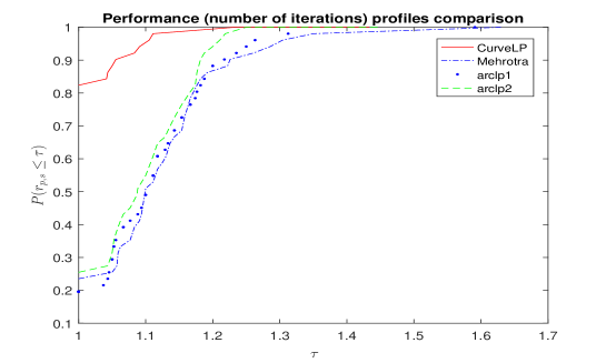
Figure 1: Performance profile comparison of the four algorithms.

8 Conclusions

In this paper, we propose two computationally efficient polynomial interior-point algorithms. These algorithms search the optimizers along ellipses that approximate the central path. The first algorithm is proved to be polynomial and its simplified version has better complexity bound than all existing infeasible interior-point algorithms and achieves the best complexity bound for all existing, feasible or infeasible, interior-point algorithms. Numerical test results for all the Netlib standard linear programming problems show that the algorithms are competitive to the state-of-the-art Mehrotra’s Algorithm which has no convergence result.

9 Acknowledgments

This is a pre-print of an article published in Numerical Algorithms. The final authenticated version is available online at: https://doi.org/10.1007/s11075-018-0469-3

The author would like to thank Dr. Chris Hoxie, in the Office of Research at US NRC, for providing computational environment for this research.

References

- [1] S. Wright, Primal-Dual Interior-Point Methods, SIAM, Philadelphia, (1997).
- [2] S. Mehrotra, On the implementation of a primal-dual interior point method, SIAM Journal on Optimization, Vol. 2, pp. 575-601 (1992).
- [3] I. Lustig, R. Marsten, and D. Shannon, Computational experience with a primal-dual interior-point method for linear programming, Linear Algebra and Its Applications, Vol. 152, pp. 191-222, (1991).
- [4] I. Lustig, R. Marsten, D. Shannon, On implementing Mehrotra’s predictor-corrector interior-point method for linear programming, SIAM journal on Optimization, Vol. 2, pp. 432-449 (1992).
- [5] R. Monteiro, I. Adler, M. Resende, A polynomial-time primal-dual affine scaling algorithm for linear and convex quadratic programming and its power series extension, Mathematics of Operations Research, Vol. 15, pp. 191-214 (1990).
- [6] M. Kojima, S. Mizuno, A. Yoshise, A polynomial-time algorithm for a class of linear complementarity problem, Mathematical Programming, Vol. 44, pp. 1-26 (1989).
- [7] M. Kojima, S. Mizuno, A. Yoshise, A primal-dual Interior-point algorithm for linear programming, in Progress in Mathematical Programming: Interior-point and Related Methods, N. Megiddo, ed., Springer-Verlag, New York, 1989.
- [8] C. Cartis, Some disadvantages of a Mehrotra-type primal-dual corrector interior-point algorithm for linear programming, Applied Numerical Mathematics, Vol. 59, pp. 1110-1119, (2009).
- [9] V. Klee, G. Minty, How good is the simplex algorithm? In: O. Shisha, (eds.) Inequalities, Vol. III, pp. 159-175, Academic Press, (1972).
- [10] L. Khachiyan, A polynomial algorithm in linear programming, Doklady Akademiia Nauk SSSR, Vol. 224, pp. 1093-1096, (1979).
- [11] N. Karmarkar, A new polynomial-time algorithm for linear programming, Combinatorica, Vol. 4, pp. 375-395, (1984).
- [12] M.J. Todd, The many facets of linear programming, Mathematical Programming, Ser. B, Vol. 91, pp. 417-436, (2002).
- [13] Y. Yang, A Polynomial Arc-Search Interior-Point Algorithm for Linear Programming, Journal of Optimization Theory and Applications, Vol. 158 (3) pp. 859-873, (2013).
- [14] Y. Yang, A polynomial arc-search interior-point algorithm for convex quadratic programming, European Journal of Operational Research, Vol. 215, 25-38, (2011).
- [15] C. Cartis, N.I.M. Gould, Finding a point in the relative interior of a polyhedron, Technical Report NA-07/01, Computing Laboratory, Oxford University, (2007).
- [16] Y. Yang, CurveLP-a MATLAB implementation of an infeasible interior-point algorithm for linear programming, Numerical Algorithms, Vol. 74 (4), pp. 967-996 (2017).
- [17] Y. Zhang, On the convergence of a class of infeasible interior-point methods for the horizontal linear complementarity problem, SIAM Journal on Optimization, Vol.4, pp. 208-227, (1994).
- [18] M. Mizuno, Polynomiality of infeasible interior-point algorithms for linear programming, Vol. 67, pp. 109-119, (1994).
- [19] J. Miao, Two infeasible interior-point predict-corrector algorithms for linear programming, SIAM J. Optim., 6(3), pp587-599, (1996).
- [20] Y. Yang and M. Yamashita, An arc-search O(nL) infeasible-interior-point algorithm for linear programming, Optimization Letters, DOI 10.1007/s11590-017-1142-9.
- [21] Kojima, M., Basic lemmas in polynomial-time infeasible interior-point methods for linear programming, Annals of Operations Research, 62, pp.1-28, (1996).
- [22] E. D. Andersen, Finding all linearly dependent rows in large-scale linear programming, Optimization methods and software, Vol. 6, pp. 219-227, 1995.
-
[23]
Y. Yang, Arc-search path-following interior-point
algorithms for linear programming, Optimization Online, August 2009.
http://www.optimization-online.org/DB_HTML/2009/08/2375.html. - [24] Y. Yang, An Efficient Polynomial Interior-Point Algorithm for Linear Programming, arXiv:1304.3677[math.OC], 2013.
- [25] M. Kojima, N. Megiddo, and S. Mizuno, A primal-dual infeasible interior-point algorithm for linear programming. Mathematical Programming, Series A, Vol. 61, pp.261-280, (1993).
- [26] J. Czyzyk, S. Mehrotra, M. Wagner, and S. J. Wright, PCx User Guide (version 1.1), Technical Report OTC 96/01, Optimization Technology Center, 1997.
- [27] Y. Zhang, Solving large-scale linear programs by interior-point methods under the Matlab environment, Technical Report TR96-01, Department of Mathematics and Statistics, University of Maryland, (1996).
- [28] E. Ng and B.W. Peyton, Block sparse Cholesky algorithm on advanced uniprocessor computers, SIAM Journal on Scientific Computing, Vol. 14, pp. 1034-1056, (1993).
- [29] J.W. Liu, Modification of the minimum degree algorithm by multiple elimination, ACM Transactions on Mathematical Software, 11, pp.141-153, (1985).
- [30] O. Guler, D. den Hertog, C. Roos, T. Terlaky and T. Tsuchiya, Degeneracy in interior-point methods for linear programming: a survey, Annals of Operations Research, 46, pp. 107-138, (1993).
- [31] P.E. Gill, W. Murray, M.A. Saunders, J.A. Tomlin, and M.H. Wright, On projected Newton barrier methods for linear programming and an equivalence of Karmarkar’s projective method, Mathematical Programming, Vol. 36, pp. 183-209, (1986).
- [32] J. Ekefer, Sequential minimax search for a maximum, Proceedings of the American Mathematical Society, Vol. 4, pp. 502-506, (1953).
- [33] D. Luenberger, Linear and Nonlinear Programming, Second Edition, Addison-Wesley Publishing Company, Menlo Park, (1984).
- [34] A.L. Tits and Y. Yang, Globally convergent algorithms for robust pole assignment by state feedback, IEEE transactions on Automatic Control, Vol. 41, pp. 1432-1452, (1996).
- [35] E.D. Dolan and J.J. More. Benchmarking optimization software with performance profiles. Mathematical Programming, Vol. 91, pp. 201-213, (2002).