Quantum emitter dipole-dipole interactions in nanoplasmonic systems

Abstract

We introduce a generalized Dicke-like model to describe two-level systems coupled with a single bosonic mode. In addition, the two-level systems mutually interact via direct dipole-dipole interaction. We apply the model to an ensemble of dye molecules coupled to a plasmonic excitation in a metallic nanoparticle and study how the dipole-dipole interaction and configurational randomness introduced to the system affect the energy spectra. Comparing the system eigenenergies obtained by our model with the light spectra from a multiple-scattering simulation, we suggest a way to identify dark modes in our model. Finally, we perform a parameter sweep in order to determine the scaling properties of the system and to classify the regions of the parameter space where the dipole-dipole interactions can have significant effects.

Surface plasmon polaritons (SPPs) are hybrid modes of electron plasma oscillations inside metals and the electromagnetic field inside and outside of the metallic structure. At resonant frequencies, which are determined by the plasma frequency of the bulk metal and the nanostructure geometry, the intensity of the SPP modes in the near field is significantly magnified. This field enhancement can lead to strong coupling between the SPP and quantum emitters (QEs) located in the vicinity of the metal surface, creating a hybrid mode consisting of the SPP and the QE excitations. The strong coupling manifests itself as an avoided crossing between the original SPP and QE energy levels, as has been experimentally realized in various nanoplasmonic structures; see (Törmä and Barnes, 2015) and for works that appeared after this review, for instance (Chikkaraddy et al., 2016; Santhosh et al., 2016; Zengin et al., 2015), and references therein.

Here we address the question whether the dipole-dipole interactions between the QEs can play a role in such systems. To our knowledge, there has not been any experimental evidence of this, but theoretical works exist that admit such possibility. A study by Salomon et al. (Salomon et al., 2012) using the FDTD solution of Maxwell-Liouville equations for a silver slit array covered by a thin layer of molecules presented a possibility for an additional mode in the transmission spectra between the avoided strong coupling modes, provided that either molecule concentration or their transition dipole moment is large enough. A multiple-scattering method based on macroscopic quantum electrodynamics was used by Delga et al. (Delga et al., 2014a, b) to show similar results for a system of single spherical nanoparticle with adjacent fluorescent molecules. Here we answer this question by a different approach, namely a modified Dicke model.

Interactions between electromagnetic fields and a collection of QEs such as atoms or fluorescent molecules are of interest in many areas of physics. The simplest quantum model of such a system is the original Dicke model (Dicke, 1954), where identical two-level systems are coupled to a single harmonic oscillator-like field mode, all with the same coupling strength, and without direct mutual coupling. Dicke model can be solved exactly using the algebraic Bethe ansatz (Gaudin, 1976). There also exists an exact solution for an extended Dicke model which includes direct coupling term between the QEs (Pan et al., 2005), but the coupling strengths between each pair of QEs must be all equal, as well as the QE–field mode couplings, which is unrealistic for real systems with many QEs. In this article, we study a model in which all the coupling strengths of both types of couplings can vary, which is expected to happen in real systems where the QEs can have various positions and orientations. The price of relaxing these constraints is the impossibility to diagonalize the Hamiltonian with the Bethe ansatz, so we use the numerical exact diagonalization instead.

The original Dicke model describes well a system of atoms in a high-Q optical nanocavity, as long as the atoms are separated well enough so that their mutual dipole-dipole interactions are negligible and the cavity supports single radiation mode near the resonant frequency of the atoms, and the other modes are well separated. However, our motivation stems from the study of nanoplasmonic systems where QEs interact with surface plasmon polariton (SPP) modes supported by a metallic nanostructure. In the nanoplasmonic systems, the coupling strengths between the QEs and the SPP vary considerably depending on the configuration of the QEs. In particular, we are interested whether the dipole-dipole couplings between the QEs can have significant effect on the system.

Approaches different from ours have been developed to model the behaviour of the nanoplasmonic systems in question. Among the notable ones are the methods based on finite-difference time-domain (FDTD) solution of Maxwell-Liuville equations (Sukharev and Nitzan, 2011) and quantum multiple-scattering methods based on macroscopic quantum electrodynamics (Wubs et al., 2004), which have their advantages and disadvantages. Most notably, they account for the ohmic losses inside the metal and the consequent line broadening which are significant in the plasmonic systems. On the other hand, our modified Dicke model is much less computationally expensive and gives intuitive understanding of the problem. We compare our model with the multiple-scattering approach in the Section III of this article.

This paper is organized as follows. In Section I we generalize the extended Dicke model (Pan et al., 2005) by relaxing its equal-coupling symmetries. In Section II we briefly sketch the principles of the multiple-scattering method, which is used as a benchmark for our model in Section III, where for some example configurations, we compare the resulting energy levels with the far-field light spectra obtained by multiple-scattering method as shown by Delga et al. (Delga et al., 2014a), observing a clear correspondence between them. Although our model does not by itself include any information about the visibility of its eigenenergies, we find an observable which identifies the dark modes. Finally, in Section IV we use our relaxed Dicke model to perform a parameter sweep in the single excitation subspace with the goal of identifying the effects of varying dipole-dipole interactions in the model and their relevance for the parameters typical in the experiments with quantum emitters near plasmonic nanostructures. In Section V, we discuss what conditions would the system have to satisfy in order to make the effects of the dipole-dipole interactions observable.

I The relaxed Dicke model

We consider an ensemble of $K$ identical quantum emitters—modeled as two-level systems (TLS)—interacting with a single field mode. Our model Hamiltonian of the system (utilizing the rotating wave approximation) is

$$H = \hbar\omega\hat{b}^{\dagger}\hat{b}+\sum_{i}\hbar\epsilon\left(\hat{S}_{i}^{z}+\frac{1}{2}\right)+\sum_{i}V_{i}\left(\hat{b}^{\dagger}\hat{S}_{i}^{-}+\hat{S}_{i}^{+}\hat{b}\right)$$ (1)

$$+\sum_{i<j}g_{ij}\left(\hat{S}_{i}^{+}\hat{S}_{j}^{-}+\hat{S}_{j}^{+}S_{i}^{-}\right),$$

where $\omega$ is the frequency of the field mode, $\epsilon$ is the resonant frequency of the atoms, $V_{i}$ is the coupling coefficient between the $i$-th atom and the field mode, and $g_{ij}$ are the coefficients of the direct interaction between the $i$th and the $j$th atom. Here $\hat{S}_{i}^{+},\hat{S}_{i}^{-}$ and $\hat{S}_{i}^{z}$ are spin-1/2 operators given by

$$\hat{S}_{i}^{+} = \left|g_{i}\right\rangle\left\langle e_{i}\right|,\quad\hat{S}_{i}^{-}=\left|e_{i}\right\rangle\left\langle g_{i}\right|,$$

$$\hat{S}_{i}^{z} = \frac{1}{2}\left(\left|e_{i}\right\rangle\left\langle e_{i}\right|-\left|g_{i}\right\rangle\left\langle g_{i}\right|\right),$$

where $\left|g_{i}\right\rangle$ and $\left|e_{i}\right\rangle$ are the ground and excited states of the $i$th atom; $\hat{b}^{\dagger},\hat{b}$ are the creation and annihilation operators of the field mode, satisfying the usual bosonic commutation relation $\left[\hat{b},\hat{b}^{\dagger}\right]=1$.

The extended Dicke model solved by Pan et al. (Pan et al., 2005) has the same form as (1) but it assumes that the dipole-dipole and dipole-field couplings are constant, $g_{ij}=g$, $V_{i}=V$ (in addition, $g_{ij}=0$ in the original Dicke model). In contrast, in our model the coupling constants in the atom-atom and atom-field interactions may vary, relaxing the symmetries which enable the Dicke model to be exactly solvable by the Bethe ansatz. On the other hand, our model provides much more realistic description of the physical systems in which we are interested. A typical realization of our model would consist of quantum emitters (e.g. dye molecules embedded into polymer matrix) in a cavity or in the vicinity of a waveguide or a nanoparticle supporting a single dominant EM field mode—meaning that for at least a certain time scale, the remainder of the electromagnetic spectrum as well as the non-radiative losses can be neglected. The quantum emitters are deposited randomly both in positions and dipole orientations, which leads to some random distribution of the dipole-dipole coupling strengths $g_{ij}$.

Due to the rotating wave approximation, the total excitation number operator $\hat{N}=\hat{b}^{\dagger}\hat{b}+\sum_{i}\left(\hat{S}_{i}^{z}+\frac{1}{2}\right)$ commutes with the Hamiltonian. The total excitation number thus remains conserved and the Hamiltonian can be diagonalized for each excitation number subspace separately, which allows us to reduce the computational requirements of diagonalization. In the following, we deal mainly with the single excitation subspace ($N=1$) which is generated by the states $\hat{b}^{\dagger}\left|g\right\rangle,\hat{S}_{i}^{+}\left|g\right\rangle$ where $\left|g\right\rangle=\left(\left|0\right\rangle\otimes\prod_{j}\left|g_{j}\right\rangle\right)$ is the ground state of the whole system and $\left|0\right\rangle$ is the vacuum of the bosonic part.

Let us describe how the Hamiltonian (1) and its parameters can be derived for a subwavelength-sized system of a plasmonic resonator and adjacent emitters. The resonator mode alone is obtained by solving macroscopic Maxwell’s equations with the respective constitutive relations. If the system is not limited to a finite volume, this usually yields a continuum of mutually orthogonal solutions with infinite mode volumes (and thus energies). This can be worked around (Fredkin and Mayergoyz, 2003) by using e.g. a quasistatic approximation (i.e. assuming infinite speed of light) where the problem is reduced to Gauß law

$$\nabla\cdot\left(\varepsilon(\omega,\mathbf{\boldsymbol{r}})\mathbf{\boldsymbol{E}}(\mathbf{\boldsymbol{r}})\right)=0$$ (2)

with appropriate boundary conditions. This approximation eliminates the losses due to the radiation and leads to discrete spectrum in $\omega$. In order to make the spectrum real, we further neglect the imaginary part of $\varepsilon(\omega,\mathbf{\boldsymbol{r}})$ for real $\omega$, thus eliminating the internal losses of the material and making the plasmonic resonator a closed system. At this point, we get from (2) a discrete set of quasistatic modes with the dynamics of a harmonic oscillator, which—after the usual quantization procedure and dropping the zero point energy—yields the resonator part of the Hamiltonian,

$$H_{\mathrm{res}}=\hbar\sum_{\lambda}\omega_{\lambda}\hat{b}_{\lambda}^{\dagger}\hat{b}_{\lambda}$$

and the electric field operator has the form

$$\hat{\mathbf{\boldsymbol{E}}}(\mathbf{\boldsymbol{r}})=\sum_{\lambda}\sqrt{\frac{\hbar\omega_{\lambda}}{2U_{\lambda}\varepsilon_{0}}}\left(\mathbf{\boldsymbol{E}}_{\lambda}(\mathbf{\boldsymbol{r}})\hat{b}_{\lambda}+\mathbf{\boldsymbol{E}}_{\lambda}^{*}\left(\mathbf{\boldsymbol{r}}\right)\hat{b}_{\lambda}^{\dagger}\right)$$ (3)

where $\omega_{\lambda},\mathbf{\boldsymbol{E}}_{\lambda}(\mathbf{\boldsymbol{r}})$ are the solutions of the classical equation (2). The operator is normalized by the quasistatic mode energies $U_{\lambda}=\varepsilon_{0}\int\mathrm{d}^{3}\mathbf{\boldsymbol{r}}\,\left|\mathbf{\boldsymbol{E}}_{\lambda}(\mathbf{\boldsymbol{r}})\right|^{2}/2$.

As for the quantum emitters, we assume they are characterized by two parameters—the resonant frequency $\epsilon$ and magnitude $\left|\mathbf{\boldsymbol{\mu}}_{i}\right|$ of their transition dipole moment—and that they have fixed positions $\mathbf{\boldsymbol{R}}_{i}$ and directions of their dipoles $\mathbf{\boldsymbol{\mu}}_{i}/\left|\mathbf{\boldsymbol{\mu}}_{i}\right|$. Hamiltonian for the QEs before introducing interactions is $H_{\mathrm{QE}}=\sum_{i}\hbar\epsilon\left(\hat{S}_{i}^{z}+\frac{1}{2}\right)$ and its dipole moment operator

$$\hat{\mathbf{\boldsymbol{\mu}}}_{i}=\mathbf{\boldsymbol{\mu}}_{i}\left(\hat{S}_{i}^{+}+\hat{S}_{i}^{-}\right).$$ (4)

Their dipoles interact with the resonator’s electric field via the term

$$H_{\mathrm{res\text{\textendash QE}}}=-\sum_{i}\hat{\mathbf{\boldsymbol{\mu}}}_{i}\cdot\hat{\mathbf{\boldsymbol{E}}}(\mathbf{\boldsymbol{R}}_{i})$$ (5)

and with each other via the quasistatic dipole-dipole interaction

$$H_{\mathrm{QE\text{\textendash}QE}}=\frac{1}{4\pi\varepsilon_{0}}\sum_{i<j}\left(\frac{\hat{\mathbf{\boldsymbol{\mu}}}_{i}\cdot\hat{\mathbf{\boldsymbol{\mu}}}_{j}}{\left|\mathbf{\boldsymbol{R}}_{i}-\mathbf{\boldsymbol{R}}_{j}\right|^{3}}-3\frac{\left[\hat{\mathbf{\boldsymbol{\mu}}}_{i}\cdot\left(\mathbf{\boldsymbol{R}}_{i}-\mathbf{\boldsymbol{R}}_{j}\right)\right]\left[\hat{\mathbf{\boldsymbol{\mu}}}_{j}\cdot\left(\mathbf{\boldsymbol{R}}_{i}-\mathbf{\boldsymbol{R}}_{j}\right)\right]}{\left|\mathbf{\boldsymbol{R}}_{i}-\mathbf{\boldsymbol{R}}_{j}\right|^{5}}\right).$$

Finally, we take $H=H_{\mathrm{res}}+H_{\mathrm{QE}}+H_{\mathrm{QE\text{\textendash QE}}}+H_{\mathrm{res\text{\textendash}QE}}$ and perform the rotating wave approximation, dropping all the terms containing $\hat{b}_{\lambda}\hat{S}_{i}^{-},\hat{b}_{\lambda}^{\dagger}\hat{S}_{i}^{+},\hat{S}_{i}^{-}\hat{S}_{j}^{-}$ or $\hat{S}_{i}^{+}\hat{S}_{j}^{+}$, obtaining

$$H = \sum_{\lambda}\hbar\omega_{\lambda}\hat{b}_{\lambda}^{\dagger}\hat{b}_{\lambda}+\sum_{i}\hbar\epsilon\left(\hat{S}_{i}^{z}+\frac{1}{2}\right)+\sum_{i,\lambda}V_{i\lambda}\left(\hat{b}_{\lambda}^{\dagger}\hat{S}_{i}^{-}+\hat{S}_{i}^{+}\hat{b}_{\lambda}\right)$$ (6)

$$+\sum_{i<j}g_{ij}\left(\hat{S}_{i}^{+}\hat{S}_{j}^{-}+\hat{S}_{j}^{+}\hat{S}_{i}^{-}\right),$$

with the coupling coefficients

$$V_{i\lambda}=\sqrt{\frac{\hbar\omega_{\lambda}}{2U_{\lambda}\varepsilon_{0}}}\hat{\mathbf{\boldsymbol{\mu}}}_{i}\cdot\hat{\mathbf{\boldsymbol{E}}}_{\lambda}(\mathbf{\boldsymbol{R}}_{i})$$

and

$$g_{ij}=\frac{1}{4\pi\varepsilon_{0}}\left(\frac{\hat{\mathbf{\boldsymbol{\mu}}}_{i}\cdot\hat{\mathbf{\boldsymbol{\mu}}}_{j}}{\left|\mathbf{\boldsymbol{R}}_{i}-\mathbf{\boldsymbol{R}}_{j}\right|^{3}}-3\frac{\left[\hat{\mathbf{\boldsymbol{\mu}}}_{i}\cdot\left(\mathbf{\boldsymbol{R}}_{i}-\mathbf{\boldsymbol{R}}_{j}\right)\right]\left[\hat{\mathbf{\boldsymbol{\mu}}}_{j}\cdot\left(\mathbf{\boldsymbol{R}}_{i}-\mathbf{\boldsymbol{R}}_{j}\right)\right]}{\left|\mathbf{\boldsymbol{R}}_{i}-\mathbf{\boldsymbol{R}}_{j}\right|^{5}}\right).$$

For practical calculations, it is usually not necessary to take into account all the resonator modes: only the modes with frequencies near enough to the resonant frequency of the QEs will significantly affect the system. Assuming there is only one such significant mode (which is also the assumption of the Dicke model), we arrive at the Hamiltonian (1).

II The scattering approach

In the following, we compare the results of our model explained above to a multiple scattering model described in (Wubs et al., 2004; Delga et al., 2014a). For details, we refer the reader to the supplement of (Delga et al., 2014a), but we outline the main properties of the model here.

The approach is based on macroscopic quantum electrodynamics, where medium (including the plasmonic resonator in our case) is modelled by a continuum of harmonic oscillators coupled to the microscopic elecromagnetic fields in a manner that (before quantization) reproduces the phenomenological constitutive relations; the electromagnetic field operators can be then expressed in terms of the classical dyadic Green’s functions (Gruner and Welsch, 1996). Adding the microscopic QEs and coupling them to these quantized fields gives rise to a Lippmann-Schwinger equation which is hard to solve if the QEs are two-level systems. Therefore, the two-level systems are approximated by harmonic oscillators, at the cost of reliability of the model for problems that involve multiple excitations. For a given initial state, e.g. some of the emitters excited, we can derive a light spectrum that can be detected in an arbitrary point of space.

In contrast to our model described in the previous section, this approach has some advantages: it gives the light spectrum—a quantity of direct experimental relevance, it accounts for the absorption in the media, and it includes the field retardation effects, keeping its validity at longer-than-wavelength scales. These features make it a good benchmark for our model. On the other hand, the multiple-scattering approach will fail to describe the effects of higher level of excitation and it is significantly slower computationally, as it requires solving a separate matrix inversion problem for each sample frequency of the outgoing light spectrum, each inversion having the same time complexity as one exact diagonalization.

III Comparison

Let us take a simple physical system in order to compare our modified Dicke model and the multiple scattering approach. The system consists of a metal nanosphere, and several molecular dipoles modelled as two-level systems nearby, as in Figure 1. The relative permittivity of the nanosphere is approximated by the Drude model, $\varepsilon(\omega)=\varepsilon_{\infty}-\frac{\omega_{p}^{2}}{\omega\left(\omega+i\gamma_{p}\right)}$ with parameters $\varepsilon_{\infty}=4.6$, $\hbar\gamma_{p}=0.001\,\mathrm{eV}$ (the plasma frequency is chosen arbitrarily low in order to create peaks comparable to the modified Dicke model spectrum), its radius is $r=7\,\mathrm{nm}$, and we vary its plasma frequency $\omega_{p}$. In the quasistatic approximation (Ruppin, 1982), $l$-th order electric multipole resonances of a nanosphere are determined by the equation $0=\varepsilon(\omega_{l})+\varepsilon_{\mathrm{b}}(l+1)/l$ where $\varepsilon_{\mathrm{b}}$ is the environment relative permittivity. In our case, the dipole resonance is thus located at $\omega_{1}=3.02\,\mathrm{eV/\hbar}$—we use this value as the mode frequency $\omega$ in the Hamiltonian (1), whereas for the multipole scattering method, we use Mie theory with the aforementioned parameters to calculate the nanosphere response.

The molecules have transition dipole moments of $\left|\mathbf{\boldsymbol{\mu}}\right|=0.19\,\mathrm{eV\cdot nm}$, they are aligned in the $z$-direction, and positioned in a plane $8\,\mathrm{nm}$ from the centre of the nanosphere. These values were chosen in order to make the molecular interactions significant. For simplicity, we include only the electric dipole response of the nanosphere, neglecting all the higher multipole terms of Mie theory, and we assume that the field has the same shape as it would have in the electrostatic case of a polarized sphere, i.e. we neglect the outward radiation. Moreover, here we place the molecules near the equatorial plane perpendicular to the $z$ axis in order to keep the interactions the $x$ and $y$ dipoles of the nanoparticle negligible. Therefore, we can model the system with the Hamiltonian (1) (otherwise the more general Hamiltonian (6) would be needed).

In Figure 1 we show the light spectrum obtained by the multiple scattering method at a point located $10\,\mathrm{\mu m}$ away from the centre of the nanoparticle together with the eigenenergies obtained from our model. There is a clear correspondence between the peaks of the light spectrum and the eigenenergies from the respective approaches. However, not every energy level has its corresponding peak in the light spectrum; we discuss these dark states in the next section.

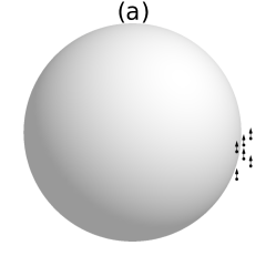
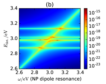
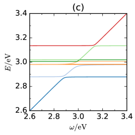
Figure 1: Configuration of the system (a) and the corresponding spectra, varying the plasma frequency of the metal: (b) far-field light spectrum obtained by the multipole scattering method, (c) eigenvalues of the Hamiltonian (1).

Characterization of the dark modes

Hamiltonian (1) describes a closed quantum system of electric dipoles with Coulombic interaction and certain internal dynamics, and by itself does not carry any information about interaction with radiation, hence nor about the visibility of its eigenstates. Therefore, we extend the system to include radiation modes and assess their visibility using perturbation theory. Let the new Hamiltonian be

$$H^{\prime}\equiv H_{0}+V=H+\sum_{\underline{\mathbf{\boldsymbol{k}}}}\hbar\omega_{\mathbf{\boldsymbol{k}}}a_{\underline{\mathbf{\boldsymbol{k}}}}^{\dagger}a_{\underline{\mathbf{\boldsymbol{k}}}}+V_{\mathrm{ext}}$$ (7)

where $\underline{\mathbf{\boldsymbol{k}}}\equiv(\mathbf{\boldsymbol{k}},\iota)$ labels the transversal (radiation) modes with mutually orthogonal wave and polarization vectors $\mathbf{\boldsymbol{k}}$ and $\mathbf{\boldsymbol{\varepsilon}}_{\mathbf{\boldsymbol{k}},\iota}$ (here $\iota=1,2$ labels the polarisation basis vectors), $\omega_{\mathbf{\boldsymbol{k}}}=c\left|\mathbf{\boldsymbol{k}}\right|$ is the corresponding mode frequency, and $V_{\mathrm{ext}}$ is the interaction between the transversal modes and all the dipoles (including the nanoparticle)

$$V_{\mathrm{ext}} =- \hat{\mathbf{\boldsymbol{E}}}^{\bot}(\mathbf{\boldsymbol{r}}=0)\cdot\hat{\mathbf{\boldsymbol{\mu}}}_{\mathrm{tot.}}$$ (8)

$$= \sum_{\underline{\mathbf{\boldsymbol{k}}}}i\sqrt{\frac{\hbar\omega_{\mathbf{\boldsymbol{k}}}}{2\varepsilon_{0}L^{3}}}\left(\mathbf{\boldsymbol{\varepsilon}}_{\underline{\mathbf{\boldsymbol{k}}}}a_{\underline{\mathbf{\boldsymbol{k}}}}-\mathbf{\boldsymbol{\varepsilon}}_{\underline{\mathbf{\boldsymbol{k}}}}a_{\underline{\mathbf{\boldsymbol{k}}}}^{\dagger}\right)\cdot\left(\mathbf{\boldsymbol{\mu}}_{\mathrm{NP}}\left(b+b^{\dagger}\right)+\sum_{i}\mathbf{\boldsymbol{\mu}}_{i}\left(S_{i}^{+}+S_{i}^{-}\right)\right).$$ (9)

Here we use the usual way to quantize transversal EM modes (Cohen-Tannoudji et al., 2000). Furthemore, we assume a cutoff in the frequencies such that $\mathbf{\boldsymbol{k}}\cdot\mathbf{\boldsymbol{r}}_{\mathrm{sys}}\ll 1$ where $\mathbf{\boldsymbol{r}}_{\mathrm{sys}}$ is the radius of the volume in which the dipoles are placed, so all the dipole positions can be replaced with $\mathbf{\boldsymbol{r}}=0$ (dipole approximation for the whole original system) and ultraviolet divergences are avoided. Finally, we assume that all the conditions to apply the Fermi’s golden rule are fulfilled. Decay rate of an initial state $\left|\alpha\right\rangle$ from the eigenspace of the original Hamiltonian $H$ into the continuum of final transversal photonic states $\left|f\right\rangle$ is proportional to the sum of squares of the corresponding transition amplitudes (Cohen-Tannoudji et al., 2000)

$$\Gamma_{\alpha}\propto\sum_{f}\left|\left\langle f\right|V_{\mathrm{ext}}\left|\alpha\right\rangle\right|^{2}.$$ (10)

To keep the length of the formulae reasonable, in the following we denote $\mathbf{\boldsymbol{\mu}}_{0}\equiv\mathbf{\boldsymbol{\mu}}_{\mathrm{NP}}$, $S_{0}^{+}\equiv b^{\dagger}$, $S_{0}^{-}\equiv b$. In the single excitation subspace (using RWA), both initial and final subspaces are spanned by the states obtained by applying a single corresponding creation operator onto the vacuum state of $H_{0}$, $\left|f\right\rangle=\left|\underline{\mathbf{\boldsymbol{k}}}\right\rangle\equiv a_{\underline{\mathbf{\boldsymbol{k}}}}^{\dagger}\left|0\right\rangle$, $\left|\alpha\right\rangle=\sum_{i=0}^{K}c_{i}S_{i}^{+}\left|0\right\rangle$. Substituting this to (10) gives

$$\Gamma_{\alpha} \propto \sum_{\underline{\mathbf{\boldsymbol{k}}}}\left\langle\alpha\right|\hat{\mathbf{\boldsymbol{\mu}}}_{\mathrm{tot.}}\cdot\sum_{\underline{\mathbf{\boldsymbol{k}}^{\prime}}}i\sqrt{\frac{\hbar\omega_{\mathbf{\boldsymbol{k}}^{\prime}}}{2\varepsilon_{0}L^{3}}}\left(\mathbf{\boldsymbol{\varepsilon}}_{\underline{\mathbf{\boldsymbol{k}}^{\prime}}}a_{\underline{\mathbf{\boldsymbol{k}}^{\prime}}}-\mathbf{\boldsymbol{\varepsilon}}_{\underline{\mathbf{\boldsymbol{k}}^{\prime}}}a_{\underline{\mathbf{\boldsymbol{k}}^{\prime}}}^{\dagger}\right)a_{\underline{\mathbf{\boldsymbol{k}}}}^{\dagger}$$

$$\times\left|0\right\rangle\left\langle 0\right|a_{\underline{\mathbf{\boldsymbol{k}}}}\sum_{\underline{\mathbf{\boldsymbol{k}}^{\prime\prime}}}-i\sqrt{\frac{\hbar\omega_{\mathbf{\boldsymbol{k}}^{\prime\prime}}}{2\varepsilon_{0}L^{3}}}\left(\mathbf{\boldsymbol{\varepsilon}}_{\underline{\mathbf{\boldsymbol{k}}^{\prime\prime}}}a_{\underline{\mathbf{\boldsymbol{k}}^{\prime\prime}}}-\mathbf{\boldsymbol{\varepsilon}}_{\underline{\mathbf{\boldsymbol{k}}^{\prime\prime}}}a_{\underline{\mathbf{\boldsymbol{k}}^{\prime\prime}}}^{\dagger}\right)\cdot\hat{\mathbf{\boldsymbol{\mu}}}_{\mathrm{tot.}}\left|\alpha\right\rangle$$

$$= -\sum_{\underline{\mathbf{\boldsymbol{k}}}}\frac{\hbar\omega_{\mathbf{\boldsymbol{k}}}}{2\varepsilon_{0}L^{3}}\left\langle\alpha\right|\hat{\mathbf{\boldsymbol{\mu}}}_{\mathrm{tot.}}\cdot\mathbf{\boldsymbol{\varepsilon}}_{\underline{\mathbf{\boldsymbol{k}}}}a_{\underline{\mathbf{\boldsymbol{k}}}}a_{\underline{\mathbf{\boldsymbol{k}}}}^{\dagger}\left|0\right\rangle\left\langle 0\right|a_{\underline{\mathbf{\boldsymbol{k}}}}a_{\underline{\mathbf{\boldsymbol{k}}}}^{\dagger}\mathbf{\boldsymbol{\varepsilon}}_{\underline{\mathbf{\boldsymbol{k}}}}\cdot\hat{\mathbf{\boldsymbol{\mu}}}_{\mathrm{tot.}}\left|\alpha\right\rangle$$

Here we used the commutativity of the photonic operators $a_{\underline{\mathbf{\boldsymbol{k}}}},a_{\underline{\mathbf{\boldsymbol{k}}}}^{\dagger}$ with the $S_{i}^{\pm}$ operators contained in $\hat{\mathbf{\boldsymbol{\mu}}}_{\mathrm{tot.}}$ together with the fact that $a_{\underline{\mathbf{\boldsymbol{k}}}}a_{\underline{\mathbf{\boldsymbol{k}}^{\prime\prime}}}\left|\alpha\right\rangle=0$ and $\left\langle 0\right|a_{\underline{\mathbf{\boldsymbol{k}}}}a_{\underline{\mathbf{\boldsymbol{k}}^{\prime\prime}}}^{\dagger}\left|0\right\rangle$ is nonzero only if $\underline{\mathbf{\boldsymbol{k}}^{\prime\prime}}=\underline{\mathbf{\boldsymbol{k}}}$. We assume that the space supporting the radiation modes is spherically symmetric, hence for the sum over $\underline{\mathbf{\boldsymbol{k}}}$ we get

$$\sum_{\underline{\mathbf{\boldsymbol{k}}}} \omega_{\mathbf{\boldsymbol{k}}}\mathbf{\boldsymbol{\varepsilon}}_{\underline{\mathbf{\boldsymbol{k}}}}a_{\underline{\mathbf{\boldsymbol{k}}}}a_{\underline{\mathbf{\boldsymbol{k}}}}^{\dagger}\left|0\right\rangle\left\langle 0\right|a_{\underline{\mathbf{\boldsymbol{k}}}}a_{\underline{\mathbf{\boldsymbol{k}}}}^{\dagger}\mathbf{\boldsymbol{\varepsilon}}_{\underline{\mathbf{\boldsymbol{k}}}}$$

$$=\sum_{\underline{\mathbf{\boldsymbol{k}}}}\omega_{\mathbf{\boldsymbol{k}}}\mathbf{\boldsymbol{\varepsilon}}_{\underline{\mathbf{\boldsymbol{k}}}}\left|0\right\rangle\left\langle 0\right|\mathbf{\boldsymbol{\varepsilon}}_{\underline{\mathbf{\boldsymbol{k}}}}$$

$$=\left|0\right\rangle\left\langle 0\right|\sum_{k}\omega_{k}\sum_{\iota=1,2}\int\mathrm{d}\Omega\,\mathbf{\boldsymbol{\varepsilon}}_{\mathbf{\boldsymbol{k}},\iota}\mathbf{\boldsymbol{\varepsilon}}_{\mathbf{\boldsymbol{k}},\iota}$$

$$=\frac{8}{3}\pi\mathbf{\boldsymbol{I}}\left|0\right\rangle\left\langle 0\right|\sum_{k}\omega_{k},$$

i.e. a multiple of the unit tensor $\mathbf{\boldsymbol{I}}$ (one way to calculate the angular integral $\int\mathrm{d}\Omega\,\mathbf{\boldsymbol{\varepsilon}}_{\mathbf{\boldsymbol{k}},\iota}\mathbf{\boldsymbol{\varepsilon}}_{\mathbf{\boldsymbol{k}},\iota}$ in the last step is to choose the unit vectors tangential to the circles of latitude and longitude for the polarisation vectors: $\mathbf{\boldsymbol{\varepsilon}}_{\mathbf{\boldsymbol{k}},1}=\mathbf{\boldsymbol{\hat{\theta}}},\mathbf{\boldsymbol{\varepsilon}}_{\mathbf{\boldsymbol{k}},2}=\mathbf{\boldsymbol{\hat{\phi}}}$). Therefore,

$$\Gamma_{\alpha} \propto \left\langle 0\right|\left(\sum_{i=0}^{K}c_{i}^{*}S_{i}^{-}\right)\sum_{j=0}^{K}\mathbf{\boldsymbol{\mu}}_{j}\left(S_{j}^{+}+S_{j}^{-}\right)\left|0\right\rangle$$

$$\cdot\left\langle 0\right|\sum_{m=0}^{K}\mathbf{\boldsymbol{\mu}}_{m}\left(S_{m}^{+}+S_{m}^{-}\right)\sum_{n=0}^{K}c_{n}S_{n}^{+}\left|0\right\rangle$$

$$= \left\langle 0\right|\sum_{i=0}^{K}c_{i}^{*}S_{i}^{-}\sum_{j=0}^{K}\mathbf{\boldsymbol{\mu}}_{j}S_{j}^{+}\left|0\right\rangle\cdot\left\langle 0\right|\sum_{m=0}^{K}\mathbf{\boldsymbol{\mu}}_{m}S_{m}^{-}\sum_{n=0}^{K}c_{n}S_{n}^{+}\left|0\right\rangle.$$

All the nonzero terms of expressions on the sides of the projector $\left|0\right\rangle\left\langle 0\right|$ are just multiples of the vacuum state, so the projector can be put away,

$$\Gamma_{\alpha}\propto\left\langle\alpha\right|\sum_{j=0}^{K}S_{j}^{+}\mathbf{\boldsymbol{\mu}}_{j}\cdot\sum_{m=0}^{K}S_{m}^{-}\mathbf{\boldsymbol{\mu}}_{m}\left|\alpha\right\rangle\equiv\left\langle\alpha\right|\hat{P}\left|\alpha\right\rangle.$$

The radiative decay rates are thus up to a constant factor given by the expectation value of an observable $\hat{P}$. The operator

$$\hat{P}=\sum_{j=0}^{K}S_{j}^{+}\mathbf{\boldsymbol{\mu}}_{j}\cdot\sum_{m=0}^{K}S_{m}^{-}\mathbf{\boldsymbol{\mu}}_{m}$$ (11)

resembles the total dipole moment squared, but it is not equal to the operator $\hat{\mathbf{\boldsymbol{\mu}}}_{\mathrm{tot.}}^{2}$ which contains a positive offset caused by the presence of terms like $S_{j}^{-}S_{j}^{+}$, causing an overall positive shift and therefore its expectation value being always positive. On the other hand, $\left\langle\alpha\right|\hat{P}\left|\alpha\right\rangle$ can be zero, which means that the state $\left|\alpha\right\rangle$ does not radiate (in the given approximation), i.e. it is a dark state.

Figure 2(c,d,e) shows the expectation values $\left\langle\alpha\right|\hat{P}\left|\alpha\right\rangle$ for the eigenstates of $H$ in the example configurations. Those states for which the expectation value is very low are indeed dark also in the results of the multiple scattering method. Moreover, the relative intensities of the brighter states correspond well to each other, $S(\alpha)/S(\beta)\approx\left\langle\alpha\right|\hat{P}\left|\alpha\right\rangle/\left\langle\beta\right|\hat{P}\left|\beta\right\rangle$, if the compared eigenstates $\left|\alpha\right\rangle,\left|\beta\right\rangle$ are well separated from others (otherwise their contributions in the total light spectrum cannot be distinguished) and if they do not contain significant contribution from the nanoparticle dipole (the emission properties of the two types of dipoles differ because of the different internal loss channels, which are however not considered in our model). This is demonstrated in Fig. 2(i) where the QEs are further away from the nanoparticle than in the other examples and they are all very close to each other, so their mutual dipole-dipole couplings $g_{ij}$ are stronger than their couplings with the nanoparticle $V_{i}$.

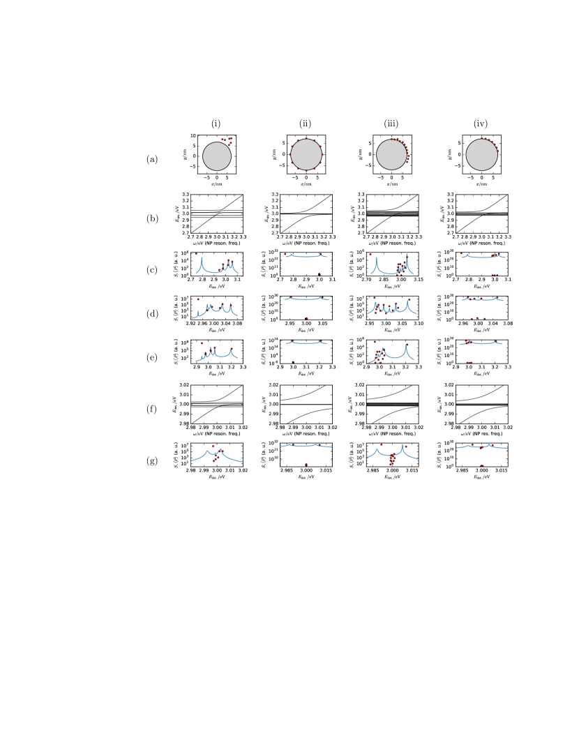
Figure 2: Example configurations (a) of quantum emitters in the equatorial plane of a spherical nanoparticle (with dipoles oriented perpendicular to the plane), the corresponding energy spectra obtained from the modified Dicke model for varying nanoparticle resonance (b), and light spectra from the multiple scattering model (blue lines, arbitrary units) together with the expectation values of the observable $\hat{P}$ for the energy eigenstates (red dots, arbitrary units) for the nanoparticle dipole resonance set at 2.8 eV (c), 3.0 eV (d) and 3.2 eV (e). The single QEs have transition energy $\hbar\epsilon=3.0\,\mathrm{eV}$ and dipole moment (c,d,e) $\mu=0.19\,\mathrm{eV\cdot nm=9.1\,D}$; the Drude damping is set to $\hbar\gamma_{\mathrm{P}}=1\,\mathrm{meV}$. Rows (f,g) are analogous to rows (b,d) but for a lower dipole moment $\mu=0.04\,\mathrm{eV\cdot nm=1.9\,D}.$

IV Exact diagonalization results

In this section, we vary the parameters of the model Hamiltonian (1) in a systematic way and compute the energy spectrum by exact diagonalization. Again, we focus only on the single-excitation subspace, i.e. the energy eigenstates satisfying $N=1$. Such states can be expressed in the form $\left|\psi\right\rangle=\left(C\hat{b}^{\dagger}+\sum_{i}c_{i}\hat{S}_{i}^{+}\right)\left|g\right\rangle$ where $c_{i},C$ are still complex coefficients.

Here we use a different way of determining $V_{i}$ than in the benchmark calculation above. We assume that the mode field is homogeneous in the volume of interest (where the QEs are), with the intensity $\mathbf{\boldsymbol{E}}$ being one of the parameters. The coupling constants are again determined as $V_{i}=-\mathbf{\boldsymbol{\mu}}_{i}\cdot\mathbf{\boldsymbol{E}}$ and are therefore dependent mainly on the orientation of a given dipole.

In the following, we study the energy spectra for varying energy $\omega$ of the bosonic field, keeping the free TLS energy difference $\epsilon$ fixed. This captures the possibility to tune the field mode, whereas the spectral properties of a molecule are given. A sample spectrum is shown in Fig. 3. Regardless of the specific configuration, in the single-excitation subspace there will generally be a bounded “band” of $K-2$ eigenvalues (where $K$ is the number of QEs) nearby the original $\epsilon$, and two “polariton branches” below and above the band asymptotically approaching $\omega$ for $\omega\ll\epsilon$ and $\omega\gg\epsilon$, respectively. The exact positions of the eigenvalues inside the band depend nontrivially on the configuration of the dipoles, but there are several quantitative attributes of the shape of the spectra—e.g. the position and the width of the band or the separation of the polariton branches—whose dependence on some basic parameters can be studied statistically.

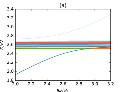
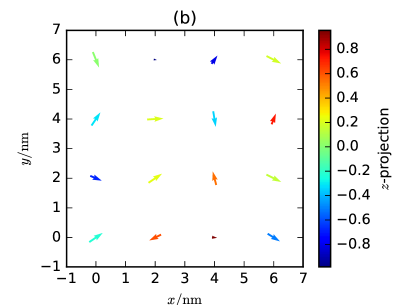
Figure 3: Sample configuration of the dipoles (b) and corresponding energy spectrum of the single-excitation subspace (a) of the modified Dicke model, with varying energy of the bosonic mode. The parameters used here are $E=E_{z}=2.4\cdot 10^{8}\,\mathrm{V\,m^{-1}}$, $\epsilon=2.6\,\mathrm{eV}/\hbar,\mu=20\,\mathrm{D}$. Here the dipoles are located in a regular $4\times 4$ square lattice but are randomly oriented. Two main polariton branches appear together with a central band of energies around the original transition frequency of a single molecule. The width of the central band grows with the dipole-dipole couplings $g_{ij}$.

Some observations about the spectra follow directly from the structure of the Hamiltonian (1). For small values of $V_{i}$, the width of the central band in the spectra is directly proportional to the dipole-dipole couplings $g_{ij}$. Therefore the width scales with the dipole moment as $\mu^{2}$ and with the length scale $l$ (proportional to the interparticle distances) as $l^{-3}$, and hence it grows linearly with the concentration of the molecules if the other parameters stay fixed. When the dipole-dipole couplings $g_{ij}$ are large enough, the lower polariton branch might cross some of the central band energies for $\omega>\epsilon$, as can be seen in Fig. 3.

The magnitude of the dipole-field couplings $V_{i}$ then affects mainly the mutual separation of the polariton branches. For small enough dipole-dipole couplings $g_{ij}$ (so that the band stays well between the polariton branches) the lower polariton branch approaches $\epsilon$ for large $\omega$, whereas there is a certain gap between the upper branch and $\epsilon$ for small $\omega$. We observe that the computed polariton branches fit quite well onto the formula

$$\tilde{\omega}_{\pm}^{2}=\frac{1}{2}\left[\omega^{2}+\omega_{0}{}^{2}+\Omega^{2}\pm\sqrt{\left(\omega^{2}+\omega_{0}{}^{2}+\Omega^{2}\right)^{2}-4\omega^{2}\omega_{0}^{2}}\right].$$ (12)

Such a dependence is found in the dispersion relations derived from several models of propagating waves (e.g. surface plasmon polaritons (Törmä and Barnes, 2015) or usual electromagnetic plane waves (Hopfield, 1958)) interacting with emitters distributed homogeneously in the direction of wave propagation and without dipole-dipole interactions. In that context, $\omega$ from (12) is the frequency of the wave of a particular wavelength in the absence of the emitters, $\omega_{0}$ is the transition frequency of the uncoupled emitters and $\Omega^{2}$ is a quantity linearly proportional to the polarisability of the emitters and also to their concentration; $\Omega$ is the Rabi splitting, equal to the difference between the polariton branches $\tilde{\omega}_{+}-\tilde{\omega}_{-}$ at resonance ($\omega=\omega_{0}$), and $\sqrt{\omega_{0}^{2}+\Omega^{2}}$ corresponds to the low-energy asymptote of the upper polariton branch.

For larger $g_{ij}$, the lower polariton branch starts to cross some of the band levels and therefore fitting the lowest eigenvalue onto $\tilde{\omega}_{-}$ is no longer reliable. Nevertheless, using only the upper branch for the fit yields still reliable results even for $\omega_{0}$. As could be seen in Fig. 2 (i,iii,iv), the shape of the lower polariton branch may still be apparent in the spectrum of the Hamiltonian even if it penetrates the central band.

In the following, we will see that neither of the parameters $\omega_{0},\Omega$ depend significantly on the dipole-dipole couplings $g_{ij}$ (cf. the section Scaling effects and Fig. (6)). The polariton splitting $\Omega$ does, however, scale with the single emitter dipole moment magnitude $\mu$ and the number of dipoles $N$ as $\Omega\propto\sqrt{\mu^{2}N}$. Therefore, the width of the central band will grow faster than the polariton splitting when the dipole concentration is increased.

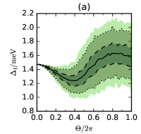
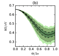
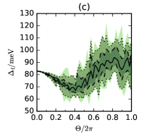
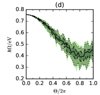
Figure 4: Effects of angular randomness on the spectrum in a $4\times 4$ dipole array ($16\,\mathrm{nm\times 16\,\mathrm{nm}}$): (a,c) width of the dipole band $\Delta_{\mathrm{f}}$ taken as the difference between the second highest and the second lowest eigenvalue at $\omega=\epsilon=2.6\,\mathrm{eV}$; (b,d) polariton splitting $\Omega$ from fitting the relation (12). The parameters are (a,c) $\mu=2\,\mathrm{D}$, $E=E_{z}=2.4\cdot 10^{9}\,\mathrm{V\,m^{-1}}$ and (b,d) $\mu=15\,\mathrm{D}$, $E=E_{z}=3.2\cdot 10^{8}\,\mathrm{V\,m^{-1}}$ (in both cases $\mu E_{z}=0.1\,\mathrm{eV}$). The lines correspond to the quantiles 0.01, 0.05, 0.25, 0.5, 0.75, 0.95, 0.99, i.e. the areas delimited by light, medium and dark shades delimit 98 %, 90 % and 50 % of the values, respectively.

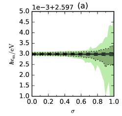
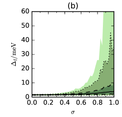
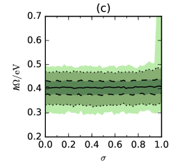
Figure 5: Effects of the position randomness on the spectrum in a $4\times 4$ dipole array ($16\,\mathrm{nm\times 16\,\mathrm{nm}}$) for $\mu=2\,\mathrm{D}$, $E=E_{z}=2.4\cdot 10^{9}\,\mathrm{V\,m^{-1}}$. The dipoles are displaced along each axis up to 1 nm. (a) center of the dipole band taken as the mean of the second highest and the second lowest eigenvalue at $\omega=\epsilon=2.6\,\mathrm{eV}$; (b) width of the dipole band $\Delta_{f}$; (c) polariton splitting $\Omega$ from fitting the relation (12). The lines correspond to the quantiles 0.01, 0.05, 0.25, 0.5, 0.75, 0.95, 0.99, i.e. the areas delimited by light, medium and dark shades delimit 98 %, 90 % and 50 % of the values, respectively.

Effects due to randomness

As mentioned in the introduction, the QEs in the nanoplasmonic system are usually distributed randomly near the metallic structures, having also random directions. In order to capture the effects of the randomness, we performed statistical simulations with varying degree of randomness in angular and positional configuration of the QEs. In both cases, we start with a rectangular array of dipoles aligned in a single direction (which corresponds to the direction of the field intensity).

We choose several statistics calculated from the resulting spectra. The width of the band can be described in multiple ways, one of them is the difference $\Delta_{\mathrm{f}}$ between the second highest and the second lowest eigenvalues at $\omega=\epsilon$. The average $\epsilon_{\mathrm{m}}$ of these two eigenvalues characterises the position of the band. For each sample, we perform a least-square fit of the spectra onto the dispersion function (12) in order to obtain the parameters $\omega_{0}$ and $\Omega$, which show the asymptotic behavior of the polariton branches and their splitting.

As for the directions, the randomness is parametrized by the maximum deviation polar angle $\Theta$. Each dipole is rotated from its aligned direction by a random polar angle chosen uniformly between $0$ and $\Theta$; the azimuth angle of the rotation is always chosen uniformly from all directions. The resulting distributions of $\Delta_{\mathrm{f}}$ and $\Omega$ are illustrated in Fig. 4 for a $4\times 4$ square array with $2\,\mathrm{nm}$ space separation with two different magnitudes of dipole moment, $2\,\mathrm{D}$ and $15\,\mathrm{D}$. The dipole-field couplings were however kept in the same range of $\pm 0.26\,\mathrm{eV}$. In all cases, the band center $\epsilon_{\mathrm{m}}$ was equal to the QE natural frequency $\epsilon$ with a relative error less than $2\cdot 10^{-4}$. The fitted value of $\omega_{0}$ was equal to $\epsilon$ with 1% accuracy (although always below the prescribed $\epsilon$).

The band width depends mainly on the magnitude of the dipole moment, $\Delta_{\mathrm{f}}\propto\mu^{2}$. The directional randomness causes variation in the band width, which in extreme cases can differ by about a factor of two for different samples.

Next, we added some noise into the dipoles’ positions. The initial configuration was a $4\times 4$ square array of randomly oriented dipoles, with $a=2\,\mathrm{nm}$ distance between dipoles. However, a random offset from the interval $(-\sigma a/2,\sigma a/2)$ was then added to each cartesian coordinate of each dipole, where $\sigma$ is a randomness parameter. The resulting distributions of selected statistics (for $\mu=2\mathrm{\,D}$) are shown in Fig. (5).

The effect of the dipole configuration on the band position is again negligible as it stays within a $1\,\mathrm{meV}$ range around the original $\epsilon$ in 90 % cases for the maximally random case. However, the band width might increase substantially for some fraction of samples in the maximally random case. This is caused by the fact that the distance between two neighbouring dipoles can approach zero and thus their mutual coupling $g_{ij}$ might become very large. As will be discussed later, this situation is mostly unphysical because of the nonzero size of the QEs. The value of $\Omega$ is apparently unaffected by the positions except for a very small fraction of cases, which again correspond to unrealistically small distances between the dipoles.

Scaling effects

In order to explore the effects of the direct dipole-dipole coupling of the QEs, we scaled the transition dipole moment relevant for the direct coupling while keeping the magnitude of $V_{i}$ coupling terms. As stated before, increasing $\mu$ by the factor of $\alpha$ is equivalent to reducing the intermolecular distance by the factor of $\alpha^{-2/3}$. The results for the scenario with the $4\times 4$ array of QEs with fixed positions at $2\,\mathrm{nm}$ interparticle distance and fully random directions is showed in Fig. 6. As expected, the band width $\Delta_{\mathrm{f}}$ shows clear quadratic dependence on $\mu$ (thus linear dependence on $g_{ij}$). The band position remains well at the QE transition frequency $\epsilon$. (Only the random fluctuations of the outermost energies of the band scale linearly with the band width, which leads to the quadratic broadening of the $\Delta_{\mathrm{f}}$ distribution with $\mu$.) The polariton splitting $\Omega$ was found to be almost independent of dipole-dipole interactions. Hence $\mu$ influences the polariton splitting only via the $V_{i}\propto\mathbf{\boldsymbol{\mu}}_{i}\cdot\mathbf{\boldsymbol{E}}(\mathbf{\boldsymbol{r}}_{i})$ terms.

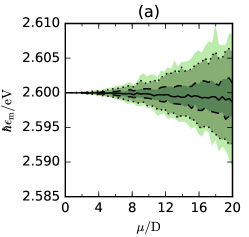
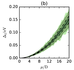
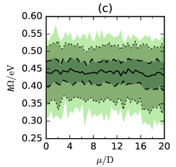
Figure 6: Scaling of the observed statistics with the transition dipole moment $\mu$, keeping the maximum field-dipole couplings fixed at $V_{i}\leq\mu E_{z}=0.1\,\mathrm{eV}$. Randomized are both dipole orientations and positions. The lines correspond to the quantiles 0.01, 0.05, 0.25, 0.5, 0.75, 0.95, 0.99, i.e. the areas delimited by light, medium and dark shades delimit 98 %, 90 % and 50 % of the values, respectively.

V Conclusions

A question naturally follows, whether the effects of the dipole-dipole interaction described above can be probed experimentally in the nanoplasmonic systems. The Hamiltonian (1), due to all the simplifications made, describes a closed system without any coupling to a probing field. We have shown, however, that the dark states are characterized by very low expectation value of the observable $P$ defined by equation (11).

The experiments showing the strong coupling between the plasmonic excitations and QEs are characterized by the observable polariton splitting. While increasing the number of QEs and their couplings to a plasmonic nanoparticle increases the polariton splitting, this does not require any direct dipole-dipole interactions between the QEs. We showed that if the dipole-dipole couplings between the QEs are present, the previously degenerate QE transition energies split into a broader band and some of the resulting states might radiate much more intensively than others. However, this requires really significant dipole-dipole coupling strengths. Larger dipole-dipole couplings can be attained by increasing the QE concentration and/or transition dipole moment. With a transition dipole moment $\mu\approx 10\,\mathrm{D}$ and separations between the emitters of $\approx 1\,\mathrm{nm}$, there should be an observable band containing highly radiant states, cf. Fig. 2(d), but such values might not be easy to attain. One of the most popular QEs used in active nanoplasmonic systems is the rhodamine 6G (R6G) dye. The number density of solid R6G is about $1.6\cdot 10^{21}\mathrm{cm^{-3}}$ (R6G, a), corresponding to the intermolecular distance of $0.86\,\mathrm{nm}$. The transition dipole moment of a separate R6G molecule is about 2 D (Penzkofer and Wiedmann, 1980). These values correspond approximately to the parameters of Fig. 2(f), where we might still expect some of the effects to be observable. However, R6G is diluted or embedded into a polymer in the experiments. The number density of $2.5\cdot 10^{19}\,\mathrm{cm}^{-3}$ and typical intermolecular separation of $3.5\,\mathrm{nm}$, corresponding to the saturated water solution of R6G (R6G, b), thus provide a more realistic estimate. For such parameters, the dipole-dipole couplings are so small that no observable effects can be expected.

Based on these arguments, we can speculate that it would be challenging but not impossible to observe effects of the direct quantum emitter dipole-dipole couplings in the nanoplasmonic systems: it demands a high value of the dipole moment concentration. Also in the paper of Salomon et al. (Salomon et al., 2012), the new mode appears in the absorption spectra for a high dipole moment value of 25 D and concentration of $10^{19}\,\mathrm{cm}^{-3}$. Note that here we studied only the single excitation subspace. It is possible that other important effects of the dipole-dipole interactions could take place for higher excitation numbers.

References

- Törmä and Barnes (2015) P. Törmä and W. L. Barnes, Rep. Prog. Phys. 78, 013901 (2015).
- Chikkaraddy et al. (2016) R. Chikkaraddy, B. de Nijs, F. Benz, S. J. Barrow, O. A. Scherman, E. Rosta, A. Demetriadou, P. Fox, O. Hess, and J. J. Baumberg, Nature 535, 127 (2016).
- Santhosh et al. (2016) K. Santhosh, O. Bitton, L. Chuntonov, and G. Haran, Nat. Commun. 7, ncomms11823 (2016).
- Zengin et al. (2015) G. Zengin, M. Wersäll, S. Nilsson, T. J. Antosiewicz, M. Käll, and T. Shegai, Phys. Rev. Lett. 114, 157401 (2015).
- Salomon et al. (2012) A. Salomon, R. J. Gordon, Y. Prior, T. Seideman, and M. Sukharev, Phys. Rev. Lett. 109, 073002 (2012).
- Delga et al. (2014a) A. Delga, J. Feist, J. Bravo-Abad, and F. Garcia-Vidal, Phys. Rev. Lett. 112, 253601 (2014a).
- Delga et al. (2014b) A. Delga, J. Feist, J. Bravo-Abad, and F. J. Garcia-Vidal, J. Opt. 16, 114018 (2014b).
- Dicke (1954) R. H. Dicke, Phys. Rev. 93, 99 (1954).
- Gaudin (1976) M. Gaudin, J. Phys. France 37, 1087 (1976).
- Pan et al. (2005) F. Pan, T. Wang, J. Pan, Y.-F. Li, and J. P. Draayer, Phys. Lett. A 341, 94 (2005).
- Sukharev and Nitzan (2011) M. Sukharev and A. Nitzan, Phys. Rev. A 84, 043802 (2011).
- Wubs et al. (2004) M. Wubs, L. G. Suttorp, and A. Lagendijk, Phys. Rev. A 70, 053823 (2004).
- Fredkin and Mayergoyz (2003) D. Fredkin and I. Mayergoyz, Phys. Rev. Lett. 91 (2003).
- Gruner and Welsch (1996) T. Gruner and D.-G. Welsch, Phys. Rev. A 53, 1818 (1996).
- Ruppin (1982) R. Ruppin, The Journal of Chemical Physics 76, 1681 (1982).
- Cohen-Tannoudji et al. (2000) C. Cohen-Tannoudji, J. Dupont-Roc, and G. Grynberg, Processus d’interaction entre photons et atomes (EDP Sciences, Les Ulis France; Paris, 2000), ISBN 978-2-86883-358-7.
- Hopfield (1958) J. J. Hopfield, Phys. Rev. 112, 1555 (1958).
- R6G (a) Rhodamine 6G, MSDS [online], ScienceLab (2013), accessed Aug 29, 2016, URL http://www.sciencelab.com/msds.php?msdsId=9927579.
- Penzkofer and Wiedmann (1980) A. Penzkofer and J. Wiedmann, Opt. Commun. 35, 81 (1980).
- R6G (b) Rhodamine 6G, Product database [online], Santa Cruz Biotech, accessed Aug 29, 2016, URL http://www.scbt.com/datasheet-280066-rhodamine-6g.html.