On Jensen’s inequality for generalized Choquet integral with an application to risk aversion

Abstract

In the paper we give necessary and sufficient conditions for the Jensen inequality to hold for the generalized Choquet integral with respect to a pair of capacities. Next, we apply obtained result to the theory of risk aversion by providing the assumptions on utility function and capacities under which an agent is risk averse. Moreover, we show that the Arrow-Pratt theorem can be generalized to cover the case, where the expectation is replaced by the generalized Choquet integral.

Keywords: Choquet integral; symetric Choquet integral; Credibility measure; Belief function, Uncertainty measure; Possibility measure; Risk aversion; Measures of risk aversion.

1 Introduction

Let $(\Omega,\mathcal{F})$ be a measurable space, where $\mathcal{F}$ is a $\sigma$-algebra of subsets of a non-empty set $\Omega.$ A (normalized) capacity on $\mathcal{F}$ is a set function $\mu\colon\mathcal{F}\to[0,1]$ such that $\mu(\emptyset)=0,$ $\mu(\Omega)=1$ and $\mu(A)\leq\mu(B)$ whenever $A\subset B.$ Capacities are also called fuzzy measures, nonadditive measures or monotone measures $\cite[cite]{[\@@bibref{}{zwang1}{}{}]}.$ We write $\overline{\mu}$ for the conjugate or dual capacity of $\mu,$ that is, $\overline{\mu}(A)=1-\mu(A^{c})$, where $A^{c}=\Omega\backslash A.$ The notion of capacity was introduced by Gustave Choquet in 1950 and has played an important role in fuzzy set theory, game theory, the rank-dependent expected utility model, the Dempster–Shafer theory, and many others [5, 42].

The generalized Choquet integral is defined as

$$C_{\mu\nu}(X)=\int_{0}^{\infty}\mu(X>t)dt-\int_{-\infty}^{0}\nu(X<t)dt,$$ (1)

provided that at least one of the two improper Riemann integrals is finite. Hereafter, $\mu(X\in A)=\mu(\{\omega\colon X(\omega)\in A\}).$ It is introduced by Tversky and Kahneman [41] for discrete random variables and is used to describe the mathematical foundations of Cumulative Prospect Theory. Two outstanding examples of generalized Choquet’s integral are: the Choquet integral $C_{\mu}:=C_{\mu\overline{\mu}}$ and the symmetric Choquet integral $\breve{C}_{\mu}:=C_{\mu\mu},$ also known as the $\breve{\hbox{S}}$ipo$\breve{\hbox{s}}$ integral (see [5, 18, 42]). If $\mu=\nu=P$ with a probability measure $P$, then the generalized Choquet integal reduces to the expectation $\mathsf{E}_{P}X.$

The Jensen inequality says that $\mathsf{E}f(X)\leq f(\mathsf{E}X)$ for any concave function $f$ and for any random variable $X$ with a finite expectation $\mathsf{E}X.$ This is one of fundamental result of the measure theory, having enormous applications in probability theory, statistics and other branch of mathematics. A lot of an extensions of this inequality is known with some additional assumptions on the function $f$ and for different integrals (see e.g. [14, 19, 22, 28, 31, 32, 33, 38, 40] and the references therein). To the best of our knowledge, the Jensen inequality for the integral (1) has not been considered so far.

The paper is organized as follows. In Section 2, we derive necessary and sufficient conditions for the capacities $\mu,\nu$ and function $f$ so that the Jensen inequality for the generalized Choquet integral holds. In Section 3, two fundamental result of the risk theory are extended. The first one deals with existence of risk aversion and the second is the Arrow-Pratt theorem. The Appendix contains several commonly encountered examples of capacities which will be useful in Sections 2 and 3.

2 Main result

Throughout the paper, we denote by $I$ any open interval containing 0, bounded or not. Write $L_{\mu\nu}^{I}$ for the set of such measurable functions $X\colon\Omega\to I$ that $C_{\mu\nu}(X)\in I.$ To prove our main result, we need the following lemma.

Lemma 1.

Given any capacities $\mu,\nu$, the integral $\eqref{choquet}$ has the following properties:

1. If "$>$" or "$<$" in (1) is replaced by "$\geq$" or "$\leq$", respectively, then the value of generalized Choquet integral does not change.

2. $C_{\mu\nu}(X)\leq C_{\mu\nu}(Y)$ if $X(\omega)\leq Y(\omega)$ for all $\omega$,

3. $C_{\mu\nu}(bX)=bC_{\nu\mu}(X)$ for $b\leq 0$ and $C_{\mu\nu}(bX)=bC_{\mu\nu}(X)$ for all $b>0$ and $X\in L_{\mu\nu},$

4. $C_{\mu\nu}(a+X)=a+C_{\mu\nu}(X)+\int\limits_{-a}^{0}\bigl{(}\mu(X>s)-\overline{\nu}(X\geq s)\bigr{)}ds$ for all $a\in\mathbb{R}.$

Proof. (C1) Let $\mu(X>t)<\mu(X\geq t)$ for some $t\in\mathbb{R}$. Then

$$\mu(X\geq t)>\mu(X>t)\geq\lim_{s\to t,s>t}\mu(X\geq s),$$

so $t$ is a point of discontinuity of the function $f(s):=\mu(X\geq s)$. Since $f$ is increasing, the set of points where $f$ is not continuous is at most countable, so $\mu(X>t)=\mu(X\geq t)$ almost everywhere. Similar reasoning shows that $\nu(X<t)=\nu(X\leq t)$ almost everywhere.

(C2) If $X\leq Y$, then by monotonicity of $\mu$ and $\nu$ we have $\mu(X>t)\leq\mu(Y>t)$ and $\nu(X<t)\geq\nu(Y<t)$ for each $t,$ which implies property C2.

(C3) It is clear that $C_{\mu\nu}(0\cdot X)=0\cdot C_{\mu\nu}(X)$. For $b>0$ we have

$$C_{\mu\nu}(bX)=\int_{0}^{\infty}\mu(X>t/b)dt-\int_{-\infty}^{0}\nu(X<t/b)dt=bC_{\mu\nu}(X),$$

By similar reasoning, $C_{\mu\nu}(bX)=bC_{\nu\mu}(X)$ for $b<0$.

(C4) For an arbitrary $a\in\mathbb{R}$ we have

$$C_{\mu\nu}(a+X) =\int_{-a}^{\infty}\mu(X>s)ds-\int_{-\infty}^{-a}\nu(X<s)ds$$

$$=C_{\mu\nu}(X)+\int_{-a}^{0}\mu(X>s)ds-\int_{0}^{-a}\nu(X<s)ds$$

$$=C_{\mu\nu}(X)+a+\int_{-a}^{0}\bigl{(}\mu(X>s)-\overline{\nu}(X\geq s)\bigr{)}ds.$$

∎

First we establish conditions under which the Jensen inequality holds.

Theorem 1.

Assume that $f\colon I\to\mathbb{R}$ is an increasing and concave function and $f(0)\geq 0.$ Then the following Jensen inequality holds for all $X\in L_{\mu\nu}^{I}$

$$C_{\mu\nu}(f(X))\leq f(C_{\mu\nu}(X))$$ (2)

if and only if $\mu\leq\overline{\nu}$, that is, $\mu(A)\leq\overline{\nu}(A)$ for all $A.$

Proof. First we show that the inequality $\eqref{Jensen}$ holds for all $X\in L_{\mu\nu}^{I}$ if and only if the following condition is valid:

(B) for all $X\in L_{\mu\nu}^{I}$ and $a\geq 0$

$$C_{\mu\nu}(a+X)\leq a+C_{\mu\nu}(X).$$ (3)

Of course, condition $B$ is necessary for $\eqref{Jensen}$ to hold as $f(x)=a+x$ is an increasing and concave function and $f(0)\geq 0$. We shall prove that the condition $B$ is also sufficient. Since $f$ is increasing and concave, we have for $x,y\in\mathbb{R}$

$$f(y)\leq f(x)+f^{\prime}(x)(y-x),$$ (4)

where $f^{\prime}(x)$ is the right-sided derivative of $f$ at $x$. As $f$ is concave on the open interval $I$, the derivative $f^{\prime}(x)$ exists and is finite for all $x\in I$ (see [24]). Moreover, $f(x)-xf^{\prime}(x)\geq 0$; to see this, put $y=0$ in (4). From (4), condition B and properties C2 and C3, we get

$$C_{\mu\nu}(f(X)) \leq C_{\mu\nu}(f(x)-f^{\prime}(x)x+f^{\prime}(x)X)$$

$$\leq f(x)-f^{\prime}(x)x+C_{\mu\nu}(f^{\prime}(x)X)$$

$$=f(x)-f^{\prime}(x)x+f^{\prime}(x)C_{\mu\nu}(X)$$ (5)

for all $x\in I$. Substituting $x=C_{\mu\nu}(X)$ in (2) we obtain $\eqref{Jensen}$, so condition B is sufficient for $\eqref{Jensen}$ to hold.

It follows from condition B and properties C1 and C4 that $\eqref{Jensen}$ is fulfilled for all $X\in L_{\mu\nu}^{I}$ if and only if for all $X\in L_{\mu\nu}^{I}$ and $a>0$ we have

$$\int_{-a}^{0}\left(\mu(X\geq s)-\overline{\nu}(X\geq s)\right)ds\leq 0.$$ (6)

Put $X=b\mathbf{1}_{A^{c}},$ where $-a<b<0$ and $A$ is any measurable set. Then the inequality $\eqref{w011}$ is of the form $(-b)(\mu(A)-\overline{\nu}(A))\leq 0$, and so $\eqref{w011}$ holds for any $A$ if and only if $\mu(A)\leq\overline{\nu}(A)$ for all $A$. ∎

For the Choquet integral $C_{\mu}(X)$ the condition $\mu\leq\overline{\nu}$ is satisfied for all capacities $\mu,\nu$. Moreover, for the symmetric Choquet integral $\breve{C}_{\mu}(X)$ the condition holds, e.g. if $\mu$ is any superadditive measure (that is, $\mu(A)+\mu(B)\leq\mu(A\cup B)$ for all $A,B$) or uncertainty measure (see the Appendix, Example 7).

Now we move to characterization the functions $f$ for which the inequality $\eqref{Jensen}$ holds. First, consider the case when both $\mu$ and $\nu$ are $\{0,1\}$-valued capacities, that is, $\mu(A),\nu(A)\in\{0,1\}$ for all $A.$

Theorem 2.

Assume that $\mu,\nu$ are $\{0,1\}$-valued capacities and $f\colon I\to\mathbb{R}$ is an increasing and continuous function such that $f(0)=0.$ Assume also that $\mu(B)=1$ and $\nu(B^{c})=1$ for some $B$. Then $C_{\mu\nu}(f(X))\leq f(C_{\mu\nu}(X))$ for all $X\in L_{\mu\nu}^{I}$ if and only if $f$ is weakly superadditive, that is, $f(a)+f(b)\leq f(a+b)$ for $a\leq 0\leq b$. If $\mu(B)=0$ or $\nu(B^{c})=0$ for an arbitrary $B,$ then the Jensen inequality holds true without any extra assumptions on $f$.

Proof. Put $b_{X}=\inf\{t\geq 0\colon\mu(X>t)=0\}$ and $a_{X}=\sup\{t\leq 0\colon\nu(X<t)=0\}$ with $X\in L_{\mu\nu}^{I}$. Clearly, $a_{X},b_{X}\in I$ and $C_{\mu\nu}(f(X))=a_{f(X)}+b_{f(X)}$. By continuity and monotonicity of $f$, we can see that

$$b_{f(X)} =\inf\{f(s)\geq 0\colon\mu(f(X)>f(s))=0\}$$

$$=\inf\{f(s)\geq 0\colon\mu(X>s)=0\}=f(b_{X})$$

and $a_{f(X)}=f(a_{X}).$ Hence, the inequality $C_{\mu\nu}(f(X))\leq f(C_{\mu\nu}(X))$ holds for all $X\in L_{\mu\nu}^{I}$ if and only if $f(a_{X})+f(b_{X})\leq f(a_{X}+b_{X})$ for all $X\in L_{\mu\nu}^{I}$. Observe that if $\mu(B)=\nu(B^{c})=1$ for some $B$, then $B\notin\{\emptyset,\Omega\}$ and we have $a_{X}=a$ i $b_{X}=b$ for $X=b\mathbf{1}_{B}+a\mathbf{1}_{B^{c}}$ with any $a\leq 0\leq b$, and so $\eqref{Jensen}$ holds if and only if $f$ is weakly superadditive.

Suppose it is not true that $\mu(B)=1$ and $\nu(B^{c})=1$ for some $B$. Therefore, it is impossible that $a_{X}<0$ and $b_{X}>0,$ and so $\eqref{Jensen}$ is valid for any $f$ as it has the form $f(a_{X})\leq f(a_{X})$ or $f(b_{X})\leq f(b_{X}).$ ∎

As far as we know, the class of weak superadditive functions has not been examined in the literature so far. Recall that $f$ is superadditive if $f(x)+f(y)\leq f(x+y)$ for all $x,y\in\mathbb{R}$. Clearly, each superadditive function is weakly superadditive, but not vice versa. For instance, let $h(x)$ be any increasing function for $x<0$ and let $h(x)=0$ for $x\geq 0$. The function $f(x)=x+h(x)$ jest weakly superadditive, but it does not have to be superadditive. The function $f(x)=x-\sqrt{(-x)_{+}}$ is weakly superadditive, but is not concave and $f(x)=\ln(1+x)$ is not weakly superadditive and concave. Still, there exist weakly superadditive and concave functions, e.g. $f(x)=1-e^{-x}$ or $f(x)=x-(-x)_{+}.$ Note that each of the functions given above is increasing, continuous and vanishes at zero.

Remark 1.

An equality holds in $\eqref{Jensen}$ if

• $\mu,\nu$ are arbitrary capacities and $X(\omega)=c$ for some $c\in I$ and for all $\omega$;
  

• $f(x)=ax$ or $f(x)=b$ for all $x\in I$, where $a\geq 0$ and $b\in I$;

• $\mu=\overline{\nu}$ and $f(x)=ax+b$ for $a,b\in\mathbb{R}.$

Theorem 2 shows that even if $\mu=\overline{\nu},$ this not guarantee that from the Jensen inequality $C_{\mu\nu}(f(X))\leq f(C_{\mu\nu}(X))$ it follows that $f$ is a concave function. In fact, let us take $\mu(A)=1$ for all $A\neq\emptyset$ and $\nu(A)=0$ for each $A\neq\Omega.$ It is obvious that $\mu=\overline{\nu}.$ Since it is not true that there exists $B$ such that $\mu(B)=1$ and $\nu(B^{c})=1,$ Theorem 2 implies that the Jensen inequality also holds for nonconcave functions $f.$ Therefore, we have to add an extra assumption on capacities $\mu,\nu$.

Theorem 3.

Suppose that $\mu\leq\overline{\nu}$ and there exists a measurable set $B$ such that $\mu(B)>0$ and $\nu(B^{c})>0.$ Given an increasing and continuous function $f\colon I\to\mathbb{R}$ such that $f(0)=0,$ if $C_{\mu\nu}(f(X))\leq f(C_{\mu\nu}(X))$ for all $X\in L_{\mu\nu}^{I}$ that takes two values, then $f$ is concave.

Proof. Set $p=\mu(B)$ and $q=\nu(B^{c}).$ Then $0<p\leq\overline{\nu}(B)=1-q<1,$ so $p,q\in(0,1).$ Put $X=a+(b-a)\mathbf{1}_{B},$ where $\mathbf{1}_{B}$ denotes the indicator function of set $B.$ As $f$ is increasing and $f(0)=0$, we have for $0\leq a<b$

$$C_{\mu\nu}(f(X))=\int_{0}^{f(b)}\mu(f(X)>t)dt=f(a)(1-p)+f(b)p.$$

Clearly, $C_{\mu\nu}(X)=a(1-p)+bp,$ so from the Jensen inequality we get $f(a)(1-p)+f(b)p\leq f(a(1-p)+bp)$ for $0\leq a<b$ with fixed value of $p\in(0,1)$. The function $-f$ is $p$-convex (see [33, p.53]). Hence, $-f$ is $J$-convex (see [25] and also [4] for an elementary proof). Since $f$ is continuous, $f$ is concave for $x\geq 0$ (cf. [24, p.133]).

For $a<b\leq 0$, we have

$$C_{\mu\nu}(f(X))=-\int_{f(a)}^{0}\nu(f(X)<t)dt=f(a)q+f(b)(1-q).$$

By the Jensen inequality, we have $f(a)q+f(b)(1-q)\leq f(aq+b(1-q)),$ so $f$ is concave for $x\leq 0$.

If $a<0<b,$ then $C_{\mu}(f(X))=f(a)q+f(b)p$, so the Jensen inequality is of the form

$$f(a)q+f(b)p\leq f(aq+bp).$$ (7)

As $f$ is continuous and concave for $x\leq 0$ and for $x\geq 0$, there exist the left-hand side derivative $f^{\prime}_{-}(0)$ and the right-hand side derivative $f^{\prime}_{+}(0).$ Substituting $b=-aq/p$ in (7), dividing both sides of $\eqref{for0}$ by $a<0$ and taking the limit as $a$ goes to zero, we obtain the inequality $f^{\prime}_{-}(0)\geq f^{\prime}_{+}(0),$ so the function $f$ is concave on the interval $I.$ ∎

Remark 2.

Note that the assumptions of Theorem 3 imply that neither $\mu$ nor $\nu$ is a $\{0,1\}$-valued capacitity (see the proof of Theorem 3). As we showed above, we cannot omit the assumptions about the existence of such set $B$ that $\mu(B)>0$ and $\nu(B^{c})>0$.

We now give a counterpart of Theorems 1 and 3 under the assumption that the inequality $\eqref{Jensen}$ holds only for nonnegative functions $X.$

Theorem 4.

Suppose that $f\colon I\to\mathbb{R}$ is an increasing and continuous function and $f(0)=0.$ Assume there exists $B$ such that $0<\mu(B)<1$. Then the inequality $\eqref{Jensen}$ holds for all $X\in L_{\mu\nu}^{[0,\infty)}$ if and only if $f$ is concave for $x\geq 0.$ Moreover, if $\mu$ is a $\{0,1\}$-valued capacity, then $\eqref{Jensen}$ is satisfied for any $X\in L_{\mu\nu}^{[0,\infty)}$ without any additional assumption on $f.$

Proof. The proof follows almost exactly as for Theorems 1 and 3, so we omit it. ∎

In Theorems 1-4 we restrict our attention to the case of an increasing and continuous function $f.$ An extension to a wider class of function is a difficult task due to the property $C3$ of the generalized Choquet integral. To the best of our knowledge, the only result in this direction is that of Girotto and Holtzer $\cite[cite]{[\@@bibref{}{Girotto}{}{}, \hbox{Theorem 2.5}]},$ where a Jensen type inequality for the integral $C_{\mu}$ was obtained.

3 Application

Consider an agent which has a nonnegative reference point $w$, e.g. an initial wealth measured in monetary terms. The agent faces a random outcome $X$ with known distribution. In this background, $X$ may be a random variable which takes both negative and positive values, which means that there is a possibility of yielding a gain from investition. If the agent decides to buy a contract for some premium $\pi$ and the outcome $X$ occurs, then it will be reimbursed and it does not influence the wealth. On the other hand, if she decides not to buy the contract, her wealth is $w-X$.

According to the von Neumann-Morgenstern theory, preferences of the agent can be described by a continuous and strictly increasing utility function $u\colon I\to\mathbb{R}$ with $u(0)=0$. The most common examples are: the exponential utility function $u(x)=1-e^{-ax}$, $a>0$; the power utility function $u(x)=(x+a)^{b}-a^{b}$, $a\geq 0$, $b>0$; the logarithmic utility function $u(x)=\ln((x+a)/a)$, $a\geq 1$; the power-expo utility function $u(x)=1-\exp(-bx^{c})$, $b,c>0$ (see [30]).

Pratt [35] suggested to use the equivalent utility principle to find the maximum premium $\pi$ which the agent is willing to pay. Then $\pi$ is the solution of the following equation

$$u(w-\pi)=\mathbb{E}u(w-X).$$ (8)

We say that the agent is risk averse, if she is willing to pay more than $\mathbb{E}X$ for an insurance contract paying out the monetary equivalent of a random outcome $X$, regardless her initial wealth $w$. One may prove that the agent is risk averse if and only if the function $u$ is concave, that is, $u(ax+(1-a)y)\geq au(x)+(1-a)u(y)$ for all $x,y$ and $0<a<1$. Moreover, if two agent have the same initial wealth and the $i$-th agent has twice differentiable utility function $u_{i},$ $i=1,2$, then the first of them is more risk averse (wants to pay not less than the other agent), if and only if $r_{u_{1}}(x)\geq r_{u_{2}}(x)$ for all $x$, where $r_{u_{i}}(x)$ is the coefficient of absolute risk aversion of the $i$-th agent defined as

$$r_{u}(x)=-\frac{u^{\prime\prime}(x)}{u^{\prime}(x)}$$ (9)

for $u\in\{u_{1},u_{2}\}.$ It is also called the Arrow-Pratt index. Similar results were obtained independently by Arrow [2] and de Finetti [29]. It is worth to note that in many books and papers, their authors give only a heuristic explanation of this result based on the approximation of premium $\pi$ by using the Taylor formula, see e.g. [8, 34]. Precise proofs can be found in $\cite[cite]{[\@@bibref{}{follmer,munk,pratt}{}{}]}.$ The studies on risk aversion were pursued by many researchers, see [9, 16, 27, 30] among others.

The aim of the paper is to generalize the two aforementioned results by replacing of the expected value with the generalized Choquet integral. Let $\pi_{u}(X,w)$ denote the premium determined from the following formula

$$u\bigl{(}w-\pi_{u}(X,w)\bigr{)}=C_{\mu\nu}(u(w-X)),$$ (10)

where $X$ is a financial outcome $X$ and $C_{\mu\nu}(X)$ is the Choquet integral with respect to capacities $\mu,\nu$. Since the function $u$ is strictly increasing and continuous, the premium $\pi_{u}(X,w)$ exists and is determined uniquely if $w-X\in\mathcal{X}_{u}$, where $\mathcal{X}_{u}$ denotes the set of such measurable functions $X\colon\Omega\to\mathbb{R}$ that $C_{\mu\nu}(X)\in I$ and $C_{\mu\nu}(u(X))\in u(I)$. The premium $\pi_{u}$ was proposed in [20, 21] in case of the capacities being Kahneman-Tverski distorted measures (see the Appendix, Example 2). A lot of properties of that premium was studied, but the problem of risk aversion measure was not examined.

Now, we are ready to extend the Arrow-Pratt result. We say that an agent is risk neutral, if the utility of her money is measured by the means of its value, that is, if her utility function is $u_{0}(x)=x$ for all $x\in\mathbb{R}$. We say that an agent with utility function $u\colon I\to\mathbb{R}$ is risk averse, if for all $w\geq 0$ and $X$ such that $w-X\in\mathcal{X}_{u}$ we have

$$\pi_{u}(X,w)\geq\pi_{0}:=C_{\nu\mu}(X)+\int_{0}^{w}\bigl{(}\overline{\nu}(X<s)-\mu(X<s)\bigr{)}ds,$$ (11)

where $\pi_{0}$ is the premium of a risk neutral agent.

Theorem 5.

An agent with a concave utility function is risk averse if and only if $\mu\leq\overline{\nu}.$ Moreover, if an agent is risk averse, $\mu\leq\overline{\nu}$ and $\mu(B),\nu(B^{c})>0$ for some $B$, then $u$ is a concave function.

Proof. Of course, $\pi_{u}(X,w)=w-u^{-1}(C_{\mu\nu}(u(w-X)))$. An agent with the function $u$ is risk averse if and only if for all $w\geq 0$ such that $w-X\in\mathcal{X}_{u}$ we have

$$C_{\mu\nu}(u(w-X))\leq u(C_{\mu\nu}(w-X)).$$ (12)

The desired result is now a simple consequence of Theorems 1 and 3. ∎

Corollary 1.

Assume that an agent with an utility function $u$ uses the Choquet integral $C_{\mu}$ to evaluation and $\mu$ is not a $\{0,1\}$-valued capacity. Then the agent is risk averse if and only if $u$ is a concave function.

Given $u,v\colon I\to\mathbb{R}$ such that $v(I)\subset I$, we say that an agent with the utility function $u$ is more risk averse than an agent with utility function $v$, if for all $w\geq 0$ such that $w-X\in\mathcal{X}_{u}\cap\mathcal{X}_{v},$ we have

$$\pi_{u}(X,w)\geq\pi_{v}(X,w).$$ (13)

Theorem 6 provides a generalization of the Arrow-Pratt Theorem in the case, when $\mu$ and $\nu$ are capacities. Recall that $r_{u}(x)$ denotes the coefficient of the absolute risk aversion $\eqref{equation}$.

Theorem 6.

Assume that $\mu\leq\overline{\nu}$ and $\mu(B),\nu(B^{c})>0$ for some $B$. Let $r_{u}$ and $r_{v}$ be the coefficients of the absolute risk aversion of concave and twice differentiable utility functions $u,v$, respectively. The following conditions are equivalent:

$(i)$ an agent with the utility function $u$ is more risk averse than an agent with utility function $v$;

$(ii)$ $u=g\circ v$ for some strictly increasing and concave function $g$;

$(iii)$ $r_{u}(x)\geq r_{v}(x)$ for all $x\in I$.

Proof. $\left(i\right)\Rightarrow\left(ii\right)$: From the assumption $\pi_{u}(X,w)\geq\pi_{v}(X,w)$ it follows that for all $w-X\in\mathcal{X}_{u}\cap\mathcal{X}_{v}$ we have

$$C_{\mu\nu}(g(Y))\leq g(C_{\mu\nu}(Y)),$$ (14)

where $g=u\circ v^{-1}$ and $Y=v(w-X).$ From Theorem 3 we conclude that $g$ is concave.
$\left(ii\right)\Rightarrow\left(i\right)$: Let $u=g\circ v$. Then, from the concavity of $g$ and from Theorem 1, for all $Y\in L_{\mu\nu}^{v(I)}$ we get

$$u(w-\pi_{u}(X,w)) =C_{\mu\nu}(g(Y))$$

$$\leq g(C_{\mu\nu}(Y))=u(w-\pi_{v}(X,w)),$$ (15)

thus $\pi_{u}(X,w)\geq\pi_{v}(X,w).$
$\left(ii\right)\Leftrightarrow\left(iii\right)$: Let $g=u\circ v^{-1}$. Function $g$ is increasing and twice differentiable, because it is a composition of functions $u$ and $v^{-1}$. Hence $g$ is concave if and only if $g^{\prime\prime}(x)\leq 0$ for $x\in v(I)$. Since for all $x$ we have

$$g^{\prime\prime}(x)=-\frac{u^{\prime}(v^{-1}(x))}{[v^{\prime}(v^{-1}(x))]^{2}}(r_{u}(v^{-1}(x))-r_{v}(v^{-1}(x)))\leq 0,$$ (16)

so $g$ is concave. ∎

Note that our proof is different from those in $\cite[cite]{[\@@bibref{}{follmer,munk,pratt}{}{}]},$ where some extra unnecessary assumptions are added, e.g. about the continuity of the Arrow-Pratt coefficient or the strict convexity of the utility function.

It was Georgescu and Kinnunen [13] and Zhou et al. [43] who first analyze the risk aversion within the framework of the Liu uncertainty theory (see $\cite[cite]{[\@@bibref{}{bliu11}{}{}]})$. They introduce the notions of uncertain expected utility, uncertain risk premium and give a counterpart of the Arrow-Pratt theorem under the uncertainty theory. The heuristic justification of the Arrow-Pratt Theorem was based on the Taylor approximation of premium. Theorems 5 and 6 generalize the results of [13, 43] for arbitrary capacities with proofs which do not use the heuristic reasonings (see Remark 3).

Example 1.

Suppose that $\mu(A)=g(P(A))$ and $\nu(A)=h(P(A))$ for each $A$, where $g,h$ are weighting functions (see Appendix, Example 2). From many empirical research it follows that $g$ is an $S-$shaped function, i.e. $g$ is concave on $[0,p]$ and is convex on $[p,1]$ for some $p\in(0,1)$. Moreover, small probabilities are overestimated and high probabilities are underestimated. The function $h$ has the same form as $g$, but it has a bit different parameters.

Tversky and Kahneman [41] propose the following weighting function

$$g(p)=\frac{p^{\gamma}}{(p^{\gamma}+(1-p)^{\gamma})^{1/\gamma}},$$

where $\gamma\in(0.28,1)$. In the empirical research the following estimation of the parameter $\gamma$ was obtained : $\gamma=0.61$ for $g$, $\gamma=0.69$ for $h$ (see [41]). Figure 1 shows a graph of $g$ (solid line) and $\overline{h}$ (dashed line) with parametres suggested by Tversky and Kahneman. Since $\overline{h}\geq g$, we have $\mu\leq\overline{\nu}$.

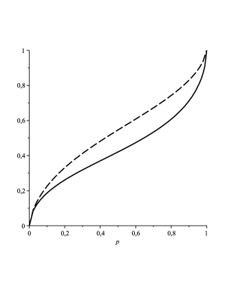
Figure 1: The Kahneman-Tversky weighting functions

Goldstein and Einhorn [15] introduce the function

$$g(p)=\frac{\delta p^{\gamma}}{\delta p^{\gamma}+(1-p)^{\gamma}}.$$

Abdellaoui [1] estimated for it values in the empirical way: $\delta=0.65$, $\gamma=0.60$ for $g$ and $\delta=0.84$, $\gamma=0.65$ for $h$. The function $g$ is depicted by a solid line and $\overline{h}$ is depicted by a dashed line in Figure 2. The condition $\mu\leq\overline{\nu}$ is satisfied.

Figure 2: The Goldstein-Einhorn weighting functions

Prelec [36] axiomatically derived the probability weighting function

$$g(x)=\exp(-\delta(-\ln p)^{\gamma}),\quad\delta>0,\;0<\gamma\leq 1.$$

Following Rieger and Wang [37], we use Perlec’s weighting function with the same parameters $\delta=1$ and $\gamma=0.74$ both for gains and for losses. The functions $g(x)$ and $\overline{h}(x)=1-g(1-x)$ are illustrated in Figure 3. The inequality $\mu\leq\overline{\nu}$ is also valid.

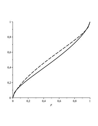
Figure 3: The Prelec weighting functions

Remark 3.

The approximation is used in the classical utility theory with probability measure $\mu$ to justify the meaning of the coefficient of risk aversion $r_{u}.$ We provide similar approximation for premium $\pi_{u}(X,w).$ From the Taylor formula at point $w$ and from $\eqref{uzytecznosc}$ we obtain

$$u(w)-u^{\prime}(w)\widehat{\pi}_{u}(X,w) =C_{\mu\nu}\bigl{(}u(w)+u^{\prime}(w)(-X)+\tfrac{1}{2}u^{\prime\prime}(w)X^{2}\bigr{)},$$

$$=u(w)-u^{\prime}(w)C_{\nu\mu}(Y)$$

$$\hskip 11.38092pt+\int_{-u(w)}^{0}\bigl{(}\mu(-u^{\prime}(w)Y>s)-\overline{\nu}(-u^{\prime}(w)Y>s)\bigr{)}ds,$$

where $\widehat{\pi}_{u}(X,w)$ denotes an approximation of premium $\pi_{u}(X,w)$ and $Y=X+r_{u}(w)X^{2}/2$. After an elementary calculation we get the following de Finetti-Arrow-Pratt approximation:

$$\widehat{\pi}_{u}(X,w)=C_{\nu\mu}(Y)+\int_{0}^{u(w)/u^{\prime}(w)}\bigl{(}\overline{\nu}(Y<t)-\mu(Y<t)\bigr{)}dt.$$ (17)

If an agent uses the Choquet integral (that is, $\mu=\overline{\nu}$), then

$$\widehat{\pi}_{u}(X,w)=C_{\overline{\mu}}(Y)\geq C_{\overline{\mu}}(X)=\pi_{0},$$ (18)

and the greater $r_{u}(w)$ measure, the greater the difference between the premium $\pi_{u}(X,w)$ and the premium of risk neutral agent is, because $Y=X+r_{u}(w)X^{2}/2$ and Choquet integral has the property C2. When the agent uses the symmetric Choquet integral $(\mu=\nu)$ and $\mu(A)+\mu(A^{c})=1$ for all $A$ (e.g. for Liu uncertainty measure, see Example 7), we have the same interpretation, because

$$\widehat{\pi}_{u}(X,w)=\breve{C}_{\mu}(Y)\geq\breve{C}_{\mu}(X)=\pi_{0}.$$

In the other cases, an interpretation of risk aversion measure via approximation (17) is not clear.

Finally, we consider an important special case, namely, when the loss $X$ does not exceed agent’s wealth.

Theorem 7.

Assume $\mu$ is not a $\{0,1\}$-valued capacity and $X(\omega)\leq w$ for all $\omega\in\Omega$. An agent with utility function $u$ is risk averse if and only if $u$ is concave for $x\geq 0$. Moreover, given concave and twice differentiable utility functions $u$ and $v$, an agent with the utility function $u$ is more risk averse than an agent with utility function $v$ if and only if $r_{u}(x)\geq r_{v}(x)$ for all $x\in I\cap[0,\infty)$.

Proof. The proof is straightforward. This follows from Theorem 4. We omit the details. ∎

4 Appendix

We give below a few commonly encountered examples of capacities.

Example 2.

Let $g\colon[0,1]\to[0,1]$ be a such non-decreasing function that $g(0)=0$ and $g(1)=1,$ called the weighting function or the distortion. The distortions of probability measure $P$ of the form $\nu(A)=g\big{(}P(A)\big{)}$ are capacities. They are crucial for the Cumulative Prospect Theory proposed by Kahneman and Tversky $\cite[cite]{[\@@bibref{}{kah}{}{}]},$ which concerns the behavior of agents on financial market using psychological aspects. It is worthy to emphasize that Kahneman was awarded with Nobel Prize in Economic Sciences in 2002 for that theory. The capacities also became a basic tool to measure risk in insurance mathematics $\cite[cite]{[\@@bibref{}{follmer, ka1,ka4}{}{}]}.$

Example 3.

Let $\mathcal{P}$ be a family of probability ditributions on $\Omega$ and let parameter $\theta\in[0,1]$ balances optimistic and pessimistic attitude of an agent. The Hurwicz capacity of the form

$$\mu^{*}(A)=\theta\inf_{P\in\mathcal{P}}P(A)+(1-\theta)\sup_{P\in\mathcal{P}}P(A),$$

is used in theory of decision making, if we have only partial information on the distribution $P$ of random outcome (see [17]).

Example 4.

The possibility measure is defined by $\mu(A)=\sup_{x\in A}\psi(x)$ for $A\neq\emptyset$, where $\psi\colon\Omega\to[0,1]$ is any such function that $\sup_{x\in\Omega}\psi(x)=1.$ The necessity measure is the conjugate of a possibility measure $\cite[cite]{[\@@bibref{}{dub,zwang1}{}{}]}.$

Example 5.

Given a nonempty subset $K$ of $\Omega,$ we call $\mu_{K}$ an unanimity game if $\mu_{K}(A)=1$ for $K\subset A$ and $\mu_{K}(A)=0$ otherwise. The set $K$ is called a coalition. Each $\{0,1\}$-valued capacity on a finite set $\Omega$ can be written as a maximum of unanimity games or as a linear combination of unanimity games with integer coefficients (see [6]).

Example 6.

A map $m\colon 2^{\Omega}\to[0,1]$ is called the mass function, if it satisfies conditions $m(\emptyset)=0$ and $\sum_{A\in 2^{\Omega}}m(A)=1$. The belief function and plausibility function are defined, respectively, as follows

$$\text{Bel}(A)=\sum_{B\subset A}m(B),\quad\quad\text{Pl}(A)=\sum_{B\cap A\neq\emptyset}m(B).$$

Both functions are examples of capacities [42]. The maps defined above play a crucial role in the Dempster-Schafer theory $\cite[cite]{[\@@bibref{}{19}{}{}]}.$

Example 7.

A map $M\colon\mathcal{F}\to[0,1]$ is called the uncertainty measure, if

1. $M(\Omega)=1,$

2. $M(A^{c})+M(A)=1$ for all $A\in\mathcal{F},$

3. $M\Big{(}\bigcup_{n=1}^{\infty}A_{n}\Big{)}\leq\sum_{n=1}^{\infty}M(A_{n})$ for any sequence $(A_{n})\subset\mathcal{F},$

This term was introduced by Liu $\cite[cite]{[\@@bibref{}{bliu11}{}{}]},$ We will show that the uncertainty measure is a capacity. A consequence of M1 and M2 is that $M(\emptyset)=0.$ If $\Omega=A^{c}\cup B,$ where $A\subset B$, then from  M1, M3 and M2 it follows that

$$1=M(X)=M(A^{c}\cup B)\leq M(A^{c})+M(B)=1-M(A)+M(B),$$

so $M$ is a monotone set function, as desired.

A particular case of uncertainty measure is the credibility measure Cr$(A)$ defined by

$$\text{Cr}(A)=\Bigl{(}\sup_{x\in A}v(x)+1-\sup_{x\in A^{c}}v(x)\Bigr{)}/2,$$ (19)

where $v\colon\Omega\to[0,1]$ is any function.

References

- [1] M. Abdellaoui, Parameter-free elicitation of utilities and probability weighting functions, Management Science 46 (2000) 1497–1512.
- [2] K.J. Arrow, Essays in the Theory of Risk Bearing, Markham Publishing Company, Chicago, 1971.
- [3] A.M.L. Casademunt, I. Georgescu, The optimal saving with mixed parameters, Procedia Economics and Finance 15 (2014) 326–333.
- [4] Z. Daróczy, Z. Páles, Convexity with given infinite weight sequences, Stochastica 11 (1987) 5–12.
- [5] D. Denneberg, Non-additive measure and integral, Kluwer Academic Publishers, Dordrecht, 1994.
- [6] D. Denneberg, Totally monotone core and products of monotone measures, International Journal of Approximate Reasoning 24 (2000) 273–281.
- [7] D. Dubois, H. Prade, Possibility Theory: An Approach to Computerized Processing of Uncertainty, Plenum Press, New York, 1988.
- [8] L. Eeckhoudt, C. Gollier, H. Schlesinger, Economic and Financial Decisions under Risk, Princeton University Press, Princeton, 2005.
- [9] H. Fllmer, A. Schied, Stochastic Finance. An Introduction in Discrete Time, De Gruyter, Berlin, 2011.
- [10] I. Georgescu, Expected utility operators and possibilistic risk aversion, Soft Computing 16 (2012) 1671–1680.
- [11] I. Georgescu, Possibility risk aversion and coinsurance problem, Fuzzy Information and Engineering 2 (2013) 221–233.
- [12] I. Georgescu, Risk aversion, prudence and mixed optimal saving models, Kybernetika 50 (2014) 706–724.
- [13] I. Georgescu, J. Kinnunen, A credibilistic approach to risk aversion and prudence, Proceedings of the Finnish Operations Research Society 40th AnniversaryWorkshop (FORS40) on Optimization and Decision-Making, Lappeenranta, Finland, August 20-21 (2013) 72–77.
- [14] B. Girotto, S. Holtzer, Chebyshev and Jensen inequalities for Choquet integral, Mathematica Pannnonica 23 (2012) 267–275.
- [15] W.M. Goldstein, H.J. Einhorn, Expression theory and the preference reversal phenomenon, Psychological Review 94 (1987) 236–254.
- [16] Ch. Gollier, The Economics of Risk and Time, MIT Press, Cambridge, 2001.
- [17] F. Gul, W. Pasendorfer, Hurwicz expected utility and subjective sources, Journal of Economic Theory 159 (2015) 465–488.
- [18] M. Grabisch, J.L. Marichal, R. Mesiar, E. Pap, Aggregation Functions, Encyclopedia of Mathematics and Its Applications 127, Cambridge University Press, Cambridge, 2009.
- [19] M.A. Khan, G.A. Khan, T. Ali, A. Kilicman, On the refinement of Jensen’s inequality, Applied Mathematics and Computation 262 (2015) 128–135.
- [20] M. Kaluszka, M. Krzeszowiec, Mean–value principle under Cumulative Prospect Theory, ASTIN Bulletin 42 (2012) 103–122.
- [21] M. Kaluszka, M. Krzeszowiec, An iterativity condition for the mean-value principle under Cumulative Prospect Theory, ASTIN Bulletin 43 (2013) 61–71.
- [22] M. Kaluszka, A. Okolewski, M. Boczek, On the Jensen type inequality for generalized Sugeno integral, Information Sciences 266 (2014) 140–147.
- [23] Lj.M. Kociæ, I.B. Lackoviæ, Convexity criterion involving linear operators. Facta Univ. (Nis̆) Ser. Mat. Inform. 1 (1986) 13–22.
- [24] M. Kuczma, An Introduction to the Theory of Functional Equations and Inequalities. Cauchy’s Equation and Jensen’s Inequality. Second edition, ed. Attila Gilányi, Birkhuser, 2009.
- [25] N. Kuhn, A note on -convex functions. In General inequalities, 4 (Oberwolfach, 1983) Internat. Schriftenreihe Numer. Math. 71, Birkhuser, Basel (1984) 269–276.
- [26] B. Liu, Uncertainty Theory, 4th Edition, Springer, Berlin, 2015.
- [27] M.J. Machina, W.K. Viscusi, Handbook of the Economics of Risk and Uncertainty, North-Holland, Amsterdam, 2014.
- [28] D. Mitrinoviæ, Classical and New Inequalities in Analysis, Springer, Berlin, 1992.
- [29] A. Montesano, De Finetti and the Arrow-Pratt Measure of Risk Aversion. Bruno de Finetti Radical Probabilist (First ed). Ed. Maria Carla Galavotti, London: College Publications (2009) 115–127.
- [30] C. Munk, Financial Asset Pricing Theory, Oxford University Press, Oxford, 2014.
- [31] C.P. Niculescu, L.E. Persson, Convex functions and their applications, Springer Science, New York, 2006.
- [32] E. Pap, M. Štrboja, Generalization of the Jensen inequality for pseudo-integral, Information Sciences 180 (2010) 543–548.
- [33] J.E. Peèariæ, F. Proschan, J.L. Tong, Convex Function, Partial Ordering and Statistical Applications, Academic Press, New York, 1991.
- [34] G. Pennacchi, Theory of Asset Pricing, Pearson Education, Boston, 2008.
- [35] J.W. Pratt, Risk aversion in the small and in the large, Econometrica 32 (1964) 122–136.
- [36] D. Prelec, The probability weighting function, Econometrica 66 (1998) 497–527.
- [37] M. Rieger, M. Wang, Cumulative prospect theory and the St. Petersburg paradox, Economic Theory 28 (2006) 665–679.
- [38] H. Román-Flores, A. Flores-Franulič, Y. Chalco-Cano, A Jensen type inequality for fuzzy integrals, Information Sciences 177 (2007) 3192–3201.
- [39] G. Shafer, A Mathematical Theory of Evidence, Princeton University Press, Princeton, 1976.
- [40] M. Štrboja, T. Grbić, I. Štajner-Papuga, G. Grujić, S. Medić, Jensen and Chebyshev inequal ities for pseudo-integrals of set-valued functions, Fuzzy Sets and Systems 222 (2013) 18–32.
- [41] A. Tversky, D. Kahneman, Advances in prospect theory: Cumulative representation of uncertainty, Journal of Risk and Uncertainty 5 (1992) 297–323.
- [42] Z. Wang, G. Klir, Generalized Measured Theory, Springer, Berlin, 2009.
- [43] J. Zhou, Y. Liu, X. Zhang, X. Gu, D. Wang (in press) Uncertain risk aversion, Journal of Intelligent Manufacturing, DOI: 10.1007/s10845-014-1013-5.