Night sky brightness at San Pedro Martir Observatory
Abstract
We present optical UBVRI zenith night sky brightness measurements collected on eighteen nights during 2013–2016 and SQM measurements obtained daily over twenty months during 2014–2016 at the Observatorio Astronómico Nacional on the Sierra San Pedro Mártir (OAN-SPM) in México. The UBVRI data is based upon CCD images obtained with the 0.84 m and 2.12 m telescopes, while the SQM data is obtained with a high-sensitivity, low-cost photometer. The typical moonless night sky brightness at zenith averaged over the whole period is U = 22.68, B = 23.10, V = 21.84, R = 21.04, I = 19.36, and SQM = 21.88 , once corrected for zodiacal light. We find no seasonal variation of the night sky brightness measured with the SQM. The typical night sky brightness values found at OAN-SPM are similar to those reported for other astronomical dark sites at a similar phase of the solar cycle. We find a trend of decreasing night sky brightness with decreasing solar activity during period of the observations. This trend implies that the sky has become darker by 0.7, 0.5, 0.3, 0.5 mag arcsec-2 since early 2014 due to the present solar cycle.
Subject headings:
atmospheric effects – light pollution – site testing – techniques: photometric – zodiacal dust1. Introduction
The Observatorio Astronómico Nacional San Pedro Mártir (hereafter OAN-SPM) is located on the top of Sierra San Pedro
Mártir in Baja California, México (2800 m, +31∘ 02” 40’ N, 115∘ 28” 00’ W).
The site excels in sky clarity with, in recent decades, approximately 70% and 80% photometric and spectroscopic time,
respectively (Tapia et al., 2007). The median seeing measured at zenith at 5000Å varies from 0.”50 to 0”.79
(Echevarría et al., 1998; Michel et al., 2003; Skidmore et al., 2009; Sánchez et al., 2012).
Atmospheric extinction is typically 0.13 mag airmass-1 in V band (Schuster and Parrao, 2001). Due to these
excellent atmospheric conditions and favorable location away from large urban areas, the OAN-SPM is an excellent
site for optical and infrared facilities.
Among the most important parameters that define the quality of an observing site it is the night sky brightness (NSB). This
parameter has been extensively studied by several authors (Kalinowski et al., 1975; Walker, 1988;
Pilachowski et al., 1989; Krisciunas et al., 1987; Leinert et al., 1995;
Mattila et al., 1996; Patat, 2003 and references therein), starting with the pioneering
work by Rayleigh (1928). In the following, we will concentrate on optical wavelengths only.
The NSB is the integrated light from two main kinds of sources: natural and artificial. Among
the sources of natural origin are airglow (recombination of molecules heated by Sun UV radiation during daytime),
aurorae, zodiacal light (sunlight scattered from interplanetary dust), diffuse galactic light (from faint unresolved
stars in our Galaxy), and the extragalactic background (due to distant, faint unresolved galaxies). The airglow and
aurorae, which originate in the Earth’s atmosphere, depend upon the site and time of the observation, while the
other three do not. The source of artificial light is mainly street lighting, with an increasing contribution
from electronic billboards and other luminous advertising media. This contribution, also known as light pollution,
is amenable to monitoring through long-term campaigns of the variation in the night sky brightness (Schneeberger et al., 1979;
Walker, 1988; Kalinowski et al., 1975; Krisciunas et al., 1987; Pilachowski et al., 1989;
Leinert et al., 1995).
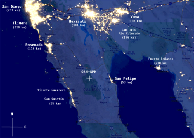
In Fig. 1 we show the cities and towns near the OAN-SPM. The cities of Ensenada and Tijuana lie between
150 and 230 km NW of OAN-SPM and have populations of 480,000 and 1.6 million people,
respectively. The city of San Diego lies 260 km distant, also to the NW, with a population of 1.3 million people.
An estimate of the contribution to the NSB due to light from nearby cities can be obtained using the
model of Garstang (1989), which provides an approximate light-pollution contribution expected from different
sources. The combined contribution of Ensenada, Tijuana and San Diego to the
sky brightness at the OAN-SPM is estimated to be less than 0.08 mag at a zenith distance of 45∘.
To the Northeast, at an average distance of 185 km, the cities of Mexicali, Yuma, and San Luis Río Colorado,
with a combined population of 1.3 million contribute with 0.04 mag. Other cities like San Felipe and San Quintín,
which are nearer to the observatory (60 km), but less populated (17 000 and 10 000 people) contribute
0.01 mag each. In Baja California, state lighting ordinances that took effect starting in 2006 in the municipality of
Ensenada and statewide in 2010 include light pollution among the environmental disturbances to be controlled.
Among its goals, this legislation seeks to reduce or at least minimize the light pollution, even with the constant
growth of its cities.
In the present paper we report UBVRI sky brightness measurements obtained on eighteen moonless nights during 2013 to 2016 and SQM sky brightness measurements collected daily during 2014 to 2016. As far as we are aware, these data constitute the largest homogeneous data set available for the OAN-SPM. The SQM data set is continuously accumulating and it will provide an unprecedented opportunity to investigate the long-term evolution of the night sky at the OAN-SPM. In Sect. 2, we present our observation procedures and reduction techniques. The results are presented in Sect. 3, while, in Sect. 4, we consider the variation of the NSB as a function of the solar activity and compare our measurements with other dark sites. Finally, in Sect. 5, we present our conclusions.
2. Observations and data reduction
2.1. CCD night sky brightness measurements
The broadband data set presented in this study was obtained with the MEXMAN and Italian filter wheels, which are
mounted at the Cassegrain focus of the 0.84 m and 2.1 m Ritchey-Chretien telescopes, respectively. The detectors are E2V
back-illuminated CCDs with 13.5 m pixels in a format, which give projected plate scales
of 0”.22/pix and 0”.18/pix at the 0.84 m and 2.1 m telescopes, respectively.
Observations of the NSB were obtained at the zenith to minimize airglow emission and extinction
on 18 photometric nights between February 2013 to May 2016 when both the Sun and Moon were at least 18∘ below
the horizon (astronomical night). Each night, a photometric standard field (Landolt, 1992) was
observed at about the same time as part of the calibration process.
Imaging frames are bias and flat-field corrected using standard reduction procedures in IRAF111IRAF is
distributed by the National Optical Astronomy Observatory, which is operated by AURA, INC. under cooperative
agreement with the National Science Foundation. Average integration times range between 600s in U band and
300s in I band, in order to obtain sufficient sky counts. Aperture photometry was performed with the APT software
(Laher et al., 2012) by using an aperture of 13∘ in areas free of nebulosity, stars, and
cosmic rays. The instrumental magnitudes of the standard stars were corrected for atmospheric extinction,
using the standard values for the OAN-SPM (Schuster and Parrao, 2001). No color correction was applied
to these magnitudes. Following the prescriptions of Pilachowski et al. (1989), the NSB is calibrated
without correcting for atmospheric extinction because we are interested in the observed brightness. The typical
average uncertainty in the photometry, neglecting the uncertainty in the exposure time and aperture size, in
our NSB measurements are 0.13, 0.05, 0.04, 0.03 and 0.02 mag for U, B, V, R, and I bands,
respectively, based upon image statistics. Our complete NSB data set from CCD imaging is tabulated in Table 6.
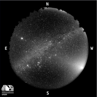
The NSB has an important contribution from zodiacal light that has to be taken into account. In
Fig. 2, we show an image of the all-sky camera installed at the OAN-SPM for the night of 18
February 2015 where we may appreciate the presence of the Milky Way at the zenith and the zodiacal light
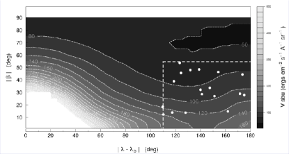
to the SW on the horizon. In Fig. 3, we have superimposed the telescope pointings on a contour plot of
the zodiacal light V brightness in helio-ecliptic coordinates (Levasseur-Regourd and Dumont, 1980), i.e., ecliptic latitude versus
the difference in ecliptic longitude of the observation and that of the Sun. We have used the equatorial celestial
coordinates at the zenith when the sky brightness was measured and
converted the right ascension and declination to helio-ecliptic coordinates. The surface brightness contours are expressed
in surface brightness units, sbu (ergs s-1 cm-2 Å-1 sr-1), e.g., a typical
V sky brightness of 21.6 mag arcsec-2 is equivalent to 366 sbu. The spectrum of the
zodiacal light is very similar to that of the Sun over the UV-IR range, and peaks at 4500 Å. In order to reduce
the scatter in our NSB measurements, we remove the zodiacal light contribution in the UBVRI passbands for each telescope
pointing (see Table 6 for the individual corrections). The average contribution to
the total NSB is 45%, 60%, 25%, 10%, and 4% in the U, B, V, R, and I bands, respectively (see Table 1).
2.2. SQM night sky brightness measurements
Since 2 November 2014, we have monitored the sky with an Unihedron Sky Quality Meter222http://www.unihedron.com
(hereafter SQM) in a continuous manner. This is a low cost NSB
photometer with high enough sensitivity to quantify the quality of the night sky at any place. The SQM is encased in
a weatherproof housing pointing at the zenith. Periodically, the housing is cleaned manually. Our study includes
data spanning 607 nights from November 2014 to June 2016, of which 534 (88%) have available data. The SQM has a
spectral response similar, though not identical, to the V band. Its sensitivity peaks at 5400 Å with a broad
transmittance window (2000 Å; see Cinzano05 for a detailed comparison with stardard photometric
systems). Here, we follow the convention of other authors and report all measurements in terms of the SQM spectral
band unit, magSQM arcsec-2.
The SQM measures the NSB every minute in a cone of about 20∘ (FWHM) and reports the result in astronomical
units of magnitudes per square arcsecond with a precision of 0.1 mag arcsec-2. Due to the large field of view,
this device detects both the zenithal and near-zenithal NSB, underestimating the true NSB of the zenith (lower
values, i.e. brighter magnitudes). This over-estimate is about mag arcsec-2, depending upon
the light pollution at the site.
Also, the SQM includes the integrated light from all stars within the field of view, which contribute approximately
6% of the NSB for stars of magnitude 5 mag and must be accounted for (Cinzano05). We do not apply
corrections for either light pollution or the integrated light of stars.
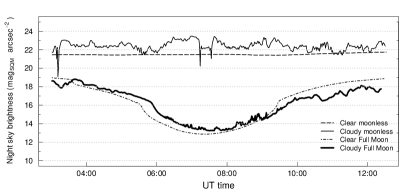
In Fig. 4, we present the SQM data plotted for four different nights: a cloudy moonless
night, a clear moonless night, a clear moonlit night, and a cloudy moonlit night, in order to show the expected
variations of the SQM data. The sky brightness on clear nights ranges from the brightest value of
13 magSQM arcsec-2 (Full Moon at 30∘ from zenith), to 21.3 magSQM arcsec-2
(Galactic plane at the zenith), to the darkest value of 22 magSQM arcsec-2 on a moonless night.
A rough estimate of the percentage of the night time (moonless and moonlit nights) free of clouds is found to
be 74%, in accord with previous studies (e.g., Tapia et al., 2007).
| Filter | NSB | NSBmin | NSBmax | NSB | ZL |
|---|---|---|---|---|---|
| (mag arcsec-2) | (mag arcsec-2) | (mag arcsec-2) | (mag arcsec-2) | (mag arcsec-2) | |
| 22.270.21 | 21.56 | 22.84 | 22.680.20 | 0.41 | |
| 22.600.15 | 22.05 | 23.26 | 23.100.12 | 0.50 | |
| 21.590.12 | 21.05 | 22.11 | 21.840.11 | 0.25 | |
| 20.900.12 | 20.36 | 21.46 | 21.040.12 | 0.14 | |
| 19.320.17 | 18.81 | 19.90 | 19.360.16 | 0.04 | |
| 21.620.16 | 21.10 | 22.04 | 21.880.15 | 0.26 |
-
•
Mean, minimum, and maximum NSB values not corrected for zodiacal light, the mean NSB corrected for zodiacal light, and the mean contribution of the zodiacal light for each filter. The is the estimated internal error of a individual measurement by subtracting off the yearly averages from the data and computing the Gaussian standard deviation of the resultant distribution.
We filter the data in several ways in order to minimize unnecessary light contributions from different sources.
First, we only consider data obtained on nights that are entirely clear. This data has been chosen
by visual inspection of All–sky camera images (see Fig. 2), resulting in 332 full nights. Second, we
select only data taken during dark time, when the Sun and Moon are at least 18∘ below the horizon. Third,
to minimize the corrections for zodiacal light, we restrict our observations to high helio-ecliptic longitudes.
Since our data set lies at ecliptic latitudes 55∘, we have applied a correction to all SQM measurements
depending on their helio-ecliptic coordinates (see Col. 7 in Table LABEL:tab:sqm) based upon the flux of the zodiacal
light in the V band (see Fig. 3). The contribution of zodiacal light is almost constant
for a given value of for 110∘, but it varies from 0.2 to
0.4 mag from to . Finally, to avoid strong contributions
from the Galactic plane, we have restricted our observations to galactic latitudes 20∘. As a
result, we retain data from 183 nights with at least 10 measurements each.
Table LABEL:tab:sqm presents all our SQM measurements as well as the zodiacal light corrections we use for each measurement.
3. Results
3.1. CCD results
In Table 1, we present the mean, minimum, and maximum values of the NSB before correction for zodiacal
light (columns 2-4), while in the last two columns we present the values of the NSB corrected for zodiacal light (column 5) and the mean value of
the zodiacal light contribution in each band (ZL, column 6). One can see from Col. 6 of Table 1 that the mean
ZL is as large as 0.5 mag in the B passband, while for the other filters this correction is smaller. For
detailed measurements of each eighteen nights and the zodiacal light correction in each filter and
observing run we refer the reader to Table 6 and Fig 12. As a by product of
our CCD sky images we have also determined the sky colors, which we present in Table 2. The NSB and
sky color uncertainties are the estimated internal error of a individual measurement by subtracting off the
yearly averages from the data and computing the Gaussian standard deviation of the resultant distribution.
For two observing runs with Moon phase and zenith distance in the range of 40∘ –60∘, we have
calculated the NSB and have found that this is on average brighter by 3.3, 3.8, 2.8, 2.1 and 0.7 magnitude in the U,
B, V, R, and I bands, respectively. In Table 2 we also give the mean sky colors obtained on
nine moonlit nights with Moon at zenithal distances in the range of 40∘ –60∘ and Moon phase .
3.2. SQM results
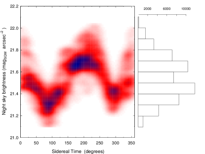
In Fig. 5 we show the NSB distribution as a function of Sidereal time before filtering for
Galactic latitude or correcting for the zodiacal light contribution. At the latitude of OAN-SPM (+31∘), the galactic
plane lies near Sidereal time 90∘ and 300∘, where it can be seen that the NSB is brighter (i.e., lower values),
with a contribution to the sky brightness of about 45% inside the field of view of the SQM due to the galactic plane.
On the other hand, in Fig. 6, we show the SQM data after filtering the data to retain only measurements
made at high galactic latitude, 20∘, and after correcting for the zodiacal light contribution. The
sky brightness variations are now dominated by the variability in the airglow
and its patchy structure. The NSB variations in individual nights, from minimum to maximum values, range between 0.1
and 0.7 magSQM arcsec-2, with a mean value of 0.20.13 magSQM arcsec-2. On a given night, the NSB
may increase, decrease, or remain constant with time. As found by Walker (1988), Pilachowski et al. (1989),
and Krisciunas (1997), on any given night the sky brightness can vary 10% to 50%. The average dispersion of the NSB on
a given night in our data is 0.06 magSQM arcsec-2 (Table LABEL:tab:sqm, column 3).
The literature is mixed on whether and how the NSB varies as a function of the time after twilight. Walker (1988)
pointed out that the sky at zenith gets darker by 0.4 mag arcsec-2 during the first six hours after the end of twilight.
On the other hand, Krisciunas (1990) found that his data obtained in the V passband showed a decrease of 0.3 mag
arcsec-2, but that this was not seen in the B passband. Other authors have not found evidence that the NSB decreases after
twilight (Leinert et al., 1995; Mattila et al., 1996; Benn and Ellison, 1998; Patat, 2003).
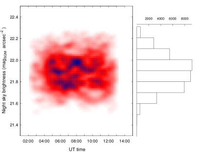
Our data agree with these last results. In Fig. 7, we present the data set from Fig. 6,
where we now plot the NSB as a function of UT time. From Fig. 7, it can be seen that there is no clear trend
in NSB after twilight (local midnight at 08:00hrs UT), as found by the work previously cited.

Besides the variations of the NSB during a single night, there are night-to night and longer-term variations.
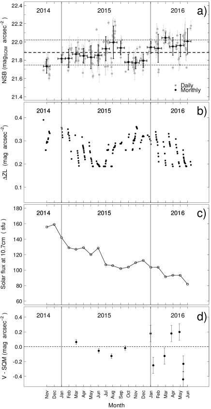
In Fig. 8a, we present daily and monthly mean NSB, which show how the NSB can vary on short
periods and to investigate any seasonal variation of the NSB. Although there is considerable variation,
Fig. 8a shows that there is no evidence for any seasonal variation of the NSB, in the sense
of a periodic variation. Instead, all the mean monthly values (black dots) are consistent with the global average given
in Table 1 (last row) and shown with horizontal dashed lines in Fig. 8a. Fig. 8b
presents the zodiacal light correction applied to the data in Fig. 8a (see Table LABEL:tab:sqm). Meanwhile,
in Fig. 8c, we plot the variation of the solar flux in the same period, which has been decreasing since 2014.
The solar flux is expected to be correlated with the NSB (see Sect. 4.1). In Fig. 8d we show the
differences between CCD V band and SQM measurements in order to check for any drift in the SQM sensor. From this figure it can be seen
that SQM and CCD measurements are comparable, with no evidence of any drift.
| Yeara | ||||
| 2013 | 2014 | 2015 | 2016 | |
| Filter | NSB | NSB | NSB | NSB |
| (mag arcsec-2) | (mag arcsec-2) | (mag arcsec-2) | (mag arcsec-2) | |
| … | ||||
| Flux⊙b | ||||
-
a
The is estimated as in Table 1. NSB values are not corrected for zodiacal light.
-
b
Solar 10.7 cm flux units 1 sfu = 104 Jy = 10-22 W m-2 Hz-1.
3.3. Variation of the NSB with Moon phase and distance
As a by product of our SQM sky brightness measurements, we performed a quantitative analysis of the data when the
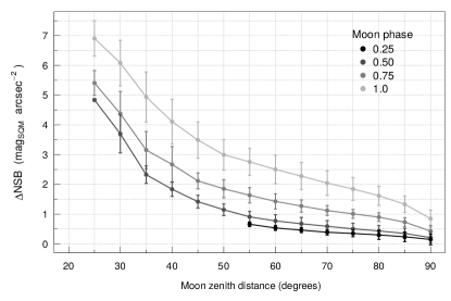
Moon is above the horizon. (For this, we use the data filtered from Table LABEL:tab:sqm.) In Fig. 9,
we show the variation in the NSB as a function of Moon phase and zenithal distance.
As expected, we find a large increase in the NSB as the zenithal distance of the Moon decreases. This variation is
naturally most extreme for the phase of full Moon. Figure 9 should be a useful tool for predicting the sky
brightness enhancement produced by the presence of the Moon at a given phase and angular distance from an observing
target, at least in the V band. Taking into account the sky colors on moonlit nights presented in Table 2,
one can see that the sky becomes bluer with the presence of the Moon. Hence, observations performed with filters bluer
than V filter, will be more affected by the Moon than redder filters.
4. Discussion
4.1. Correlation of the NSB with solar activity
A correlation between the intensity of the [O i] 5577 Å airglow line with the sunspot number was reported by
Rayleigh (1928) and Rayleigh and Jones (1935). There is now a well-established correlation with solar activity
for this and other emission lines, like [O i] 5777, 6300, 6364 Å, [O ii] 7320, 7330 Å, Na D 5890, 5896 Å, and OH
(Abreu et al., 1980; Yee et al., 1981; Takahashi et al., 1984). Walker (1988)
also found that there is a correlation between the brightness of the for V and B photometric bands with the solar 10.7 cm
radio flux (an indicator of the solar activity), demonstrating that the correlation between sky brightness and solar
activity applies not only for emission lines, but also for the airglow “pseudo continuum” emission. This correlation
has been confirmed in other studies (Pilachowski et al., 1989; Leinert et al., 1995;
Mattila et al., 1996; Krisciunas, 1997).
In order to study this correlation with solar activity in our data, Table 3 presents the mean NSB for each
year of our study. The last row of the table presents the solar 10.7 cm flux values “observed”, i.e., not corrected
to 1 AU solar distance, and averaged over the months in which our NSB observations were made. The solar fluxes are public
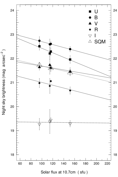
and provided by the Natural Resources Canada333http://www.spaceweather.gc.ca. In Fig. 10,
we plot the yearly average NSB values for the UBVRI filters and the SQM sensor for 2013–2016 against the solar 10.7 cm flux (solar
flux unit; 1 sfu = 10-22 W m-2 Hz-1). We also shown the linear least squares fit to CCD data in each
filter (solid lines) and SQM data (dotted line). Our data are from cycle #24 of the Sun, whose maximum was in early 2014.
The Sun’s activity has been decreasing since then, so we might expect the sky to be darker for the next five years as the Sun
passes through the minimum in the current cycle.
| Filter | a | b | r | P |
|---|---|---|---|---|
-
•
a and b are the slope and intercept, respectively, of the linear fit, , r is the correlation coefficient, and P is the probability of obtaining the result by chance.
In Table 4 we present the parameters for the least squares fits shown in Fig. 10,
with values of the NSB in each filter and the solar 10.7 cm flux, , taken from Table 3.
The correlations in Table 4
indicate that there is a trend in which the NSB in the UBVR and SQM bands () decreases as the
solar activity decreases (i.e., lower solar flux), as has been found previously. These trends have a high statistical
significance () only for the UB and SQM bands. The U and B bands are nearly devoid of emission lines
from the sky. That the significance is lower for the VR bands compared to the SQM-band data is likely the result of
the much larger number of data averaged in the latter case, given that the slopes are similar in the three cases.
Since 1947, the minimum and maximum of the monthly average solar 10.7 cm flux are approximately 60 and 250 sfu444Monthly
averages from 1947 to 2016 reported by the Natural Resources Canada.. If we consider these extreme values and the slopes
reported in Table 4, the total variation in NSB due to the solar activity over a complete cycle would be 1.8, 1.2, 0.7,
and 1.1 mag in the UBVR bands, respectively, and 0.9 mag for SQM band. The current solar cycle has been less active,
varying from a maximum of approximately 162 sfu in early 2014 to 82 sfu in recent months. This implies that, since early 2014,
the NSB at the OAN-SPM has decreased by , , , and
mag arcsec-2, respectively, based upon the slopes in Table 4.
4.2. Comparison with other observing sites
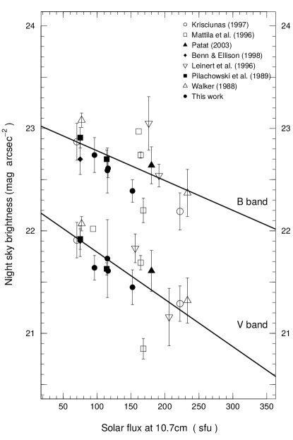
When comparing our measurements with the NSB from other observatories, we must account for the solar activity at
the time all of the measurements were made. In Table 5, we compare our minimum and maximum
NSB obtained in 2014 and 2016, respectively (see Table 3), at the OAN-SPM with broad band UBVRI values
available in the literature for other observatories. In Fig. 11,
we plot the data for the BV bandpasses from Table 5. This presentation shows that the NSB measured
at all of these sites are similar once account is taken of the solar activity.
In Fig. 11, we also show a linear fit to the data in order to determine
the expected variation of the NSB due to solar activity. The fit parameters, correlation coefficients, and
probability that they arise by chance are presented in Table 4.2. Although there is a lot of
scatter, the large number of points lead to a robust fit. The dispersion about the fits in
Table 4.2 is not surprising, as it is similar to that found
in the monthly time bins in our SQM data (Fig. 8 and Table LABEL:tab:sqm).
From Table 4.2, we estimate a maximum variation over a solar cycle of 0.6 mag and 0.9 mag in
the B and V bands, respectively, supposing that the solar activity varies from a minimum of 60 sfu to a maximum of 250 sfu.
| Site | NSBU | NSBB | NSBV | NSBR | NSBI | Flux⊙a | Ref. |
| (sfu) | |||||||
| OAN-SPM | 1 | ||||||
| Hawaii | … | … | … | 2 | |||
| … | … | … | |||||
| La Silla | … | … | … | 3 | |||
| … | … | … | |||||
| … | … | … | … | ||||
| … | … | … | … | ||||
| Paranal | 4 | ||||||
| La Palma | 5 | ||||||
| Calar Alto | … | … | … | … | 6 | ||
| … | … | … | … | ||||
| … | … | … | … | ||||
| … | … | … | … | ||||
| Kitt Peak | … | … | … | 7 | |||
| … | … | … | |||||
| San Benito Mt. | … | … | … | 8 | |||
| … | … | … |
-
•
NSB values are not corrected for zodiacal light contribution.
-
a
Solar 10.7 cm flux units 1 sfu = 104 Jy = 10-22 W m-2 Hz-1.
- •
Correlations of NSB with solar activity for data in Fig. 11 Filter a b r P
-
•
Columns 2 through 5 present, the slope (a), intercept (b), correlation coefficient (r), and the probability (P) for the least-squares fit of a linear relation for each filter, . Column 6 presents the standard deviation () about this fit.
5. Summary and conclusions
We obtained UBVRI photometry of the night sky brightness (NSB) during 18 nights from 2013 to 2016 and SQM measurements
on a daily basis from 2014 to 2016 at the Observatorio Astronómico Nacional on the Sierra San Pedro Mártir (OAN-SPM).
We have taken into account contributions to the sky brightness due to zodiacal light and have excluded observations at
low galactic latitudes in order to compare our data to those obtained at other sites. We find no clear trend of the
NSB as a function of time after twilight. The dispersion of NSB measurements over the course of a night is typically
0.2 mag, based upon our SQM data.
We investigate the long term variations of the NSB and its correlation with solar activity. We find a trend of
decreasing NSB with decreasing solar activity in the UBVR and SQM bands, though the trend is statistically
robust only for the UB and SQM bands, perhaps due to too few data points in the VR bands.
We compare the NSB at the OAN-SPM with measurements made elsewhere and find that the NSB at the OAN-SPM is comparable
to that of other observing sites. When comparing data from different observatories, we find a strong correlation
between the NSB and the solar flux at the time the measurements were made, which can be useful to estimate the
expected increase in the NSB due to solar actvity for any site. The variation in the NSB due to solar activity
can be as high as 0.6 and 0.9 mag (B and V bands) from the maximum (250 sfu) to the minimum (60 sfu) of the solar cycle.
The NSB data presented here should be useful for long-term monitoring of the quality of OAN-SPM site, which remains
one of the darkest sites in use and for future large telescope facilities.
References
- Abreu et al. (1980) Abreu, V. J., Skinner, W. R., and Hays, P. B. 1980, Geophys. Res. Lett., 7, 109
- Benn and Ellison (1998) Benn, C. R. and Ellison, S. L. 1998, New A Rev., 42, 503
- Cinzano (2005) Cinzano, P. 2005, ISTIL Internal Report, 9
- Echevarría et al. (1998) Echevarría, J., Tapia, M., Costero, R., Salas, L., Michel, R., Rojas, M. A., Muñoz, R., Valdez, J., Ochoa, J. L., Palomares, J., Harris, O., Cromwell, R. H., Woolf, N. J., Persson, S. E., and Carr, D. M. 1998, Rev. Mexicana Astron. Astrofis., 34, 47
- Garstang (1989) Garstang, R. H. 1989, PASP, 101, 306
- Kalinowski et al. (1975) Kalinowski, J. K., Roosen, R. G., and Brandt, J. C. 1975, PASP, 87, 869
- Krisciunas (1990) Krisciunas, K. 1990, PASP, 102, 1052
- Krisciunas (1997) Krisciunas, K. 1997, PASP, 109, 1181
- Krisciunas et al. (1987) Krisciunas, K., Sinton, W., Tholen, K., Tokunaga, A., Golisch, W., Griep, D., Kaminski, C., Impey, C., and Christian, C. 1987, PASP, 99, 887
- Laher et al. (2012) Laher, R. R., Gorjian, V., Rebull, L. M., Masci, F. J., Fowler, J. W., Helou, G., Kulkarni, S. R., and Law, N. M. 2012, PASP, 124, 737
- Landolt (1992) Landolt, A. U. 1992, AJ, 104, 340
- Leinert et al. (1995) Leinert, C., Vaisanen, P., Mattila, K., and Lehtinen, K. 1995, A&AS, 112, 99
- Levasseur-Regourd and Dumont (1980) Levasseur-Regourd, A. C. and Dumont, R. 1980, A&A, 84, 277
- Mattila et al. (1996) Mattila, K., Vaeisaenen, P., and Appen-Schnur, G. F. O. V. 1996, A&AS, 119, 153
- Michel et al. (2003) Michel, R., Echevarría, J., Costero, R., and Harris, O. 2003, Rev. Mexicana Astron. Astrofis., 19, 37
- Patat (2003) Patat, F. 2003, A&A, 400, 1183
- Pilachowski et al. (1989) Pilachowski, C. A., Africano, J. L., Goodrich, B. D., and Binkert, W. S. 1989, PASP, 101, 707
- Rayleigh (1928) Rayleigh, L. 1929, Proceedings of the Royal Society of London Series A, 119, 11
- Rayleigh and Jones (1935) Rayleigh, L. and Jones, H. S. 1935, 151, 222
- Sánchez et al. (2012) Sánchez, L. J., Cruz-González, I., Echevarría, J., Ruelas-Mayorga, A., García, A. M., Avila, R., Carrasco, E., Carramiñana, A., and Nigoche-Netro, A. 2012, MNRAS, 426, 635
- Schneeberger et al. (1979) Schneeberger, T. J., Worden, S. P., and Beckers, J. M. 1979, PASP, 91, 530
- Schuster and Parrao (2001) Schuster, W. J. and Parrao, L. 2001, Rev. Mexicana Astron. Astrofis., 37, 187
- Skidmore et al. (2009) Skidmore, W., Els, S., Travouillon, T., Riddle, R., Schöck, M., Bustos, E., Seguel, J., and Walker, D. 2009, PASP, 121, 1151
- Takahashi et al. (1984) Takahashi, H., Sahai, Y., and Batista, P. P. 1984, Planet. Space Sci., 32, 897
- Tapia et al. (2007) Tapia, M., Cruz-González, I., Hiriart, D., and Richer, M. 2007, Rev. Mexicana Astron. Astrofis., 31, 47
- Walker (1988) Walker, M. F. 1988, PASP, 100, 496
- Yee et al. (1981) Yee, J. H., Abreu, V. J., and Hays, P. B. 1981, J. Geophys. Res., 86, 1564
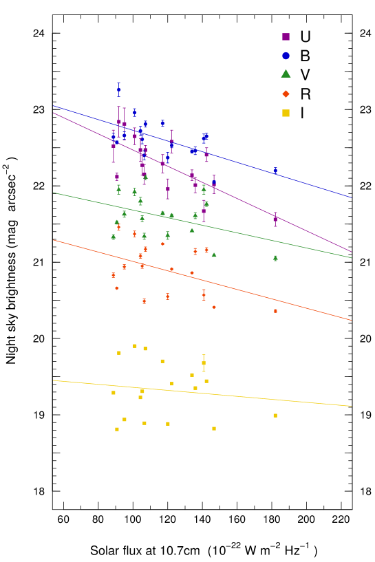
Appendix A Measurements of CCD Night sky brightness
Table 6 presents all of the NSB measurements made using CCD images from 18 nights during the years 2013-2016. Columns 1 and 2 are the UT date and time of the measurements. Cols. 3-7 present the NSB measurements in the UBVRI bands, respectively, uncorrected for the contribution of the zodiacal light. In parentheses in these columns, we present the correction for zodiacal light for each individual measurement. Column 8 presents the “observed” solar 10.7 cm flux measured on the previous UT date of the measurement. Figure 12 presents these data as a function of the solar 10.7 cm flux.
| UT Date | UT | NSBU (ZL) | NSBB (ZL) | NSBV (ZL) | NSBR (ZL) | NSBI (ZL) | Flux⊙a |
| (hh:mm) | |||||||
| 2013 | |||||||
| 18 Feb | 10:29 | 22.47(0.37) | 22.81(0.48) | 22.11(0.24) | 21.17(0.13) | 19.87(0.03) | 107 |
| 2 Apr | 04:05 | 21.96(0.50) | 22.37(0.64) | 21.35(0.32) | 20.55(0.18) | 18.88(0.05) | 120 |
| 2014 | |||||||
| 28 Jan | 11:07 | 22.41(0.38) | 22.65(0.48) | 21.76(0.24) | 21.16(0.13) | 19.44(0.03) | 142 |
| 29 Mar | 04:45 | 22.02(0.50) | 22.05(0.61) | 21.09(0.31) | 20.41(0.19) | 18.82(0.05) | 147 |
| 24 Apr | 04:29 | 22.14(0.48) | 22.45(0.60) | 21.41(0.31) | 20.86(0.17) | 19.52(0.05) | 134 |
| 15 Sep | 05:28 | 21.67(0.33) | 22.62(0.44) | 21.95(0.21) | 20.57(0.11) | 19.68(0.03) | 140 |
| 28 Oct | 09:11 | 21.56(0.37) | 22.20(0.47) | 21.05(0.23) | 20.36(0.13) | 18.99(0.03) | 182 |
| 2015 | |||||||
| 17 Mar | 08:10 | 22.29(0.45) | 22.82(0.55) | 21.64(0.29) | 21.24(0.16) | 19.70(0.04) | 117 |
| 17 Jun | 05:33 | 22.01(0.32) | 22.46(0.42) | 21.61(0.19) | 21.14(0.10) | 19.35(0.03) | 136 |
| 8 Aug | 06:23 | 22.58(0.53) | 22.53(0.41) | 21.61(0.26) | 20.91(0.14) | 19.41(0.04) | 122 |
| 3 Oct | 03:22 | 22.27(0.30) | 22.61(0.40) | 21.57(0.19) | 20.95(0.10) | 19.31(0.03) | 105 |
| 2016 | |||||||
| 15 Jan | 09:24 | 22.47(0.50) | 22.72(0.64) | 21.80(0.32) | 21.08(0.18) | 19.23(0.05) | 104 |
| 26 Jan | 02:54 | 22.15(0.56) | 22.40(0.69) | 21.34(0.35) | 20.49(0.20) | 18.89(0.05) | 107 |
| 12 Mar | 08:53 | 22.81(0.45) | 22.66(0.55) | 21.63(0.29) | 20.94(0.16) | 18.94(0.04) | 95 |
| 9 Apr | 09:39 | 22.65(0.35) | 22.96(0.46) | 21.92(0.21) | 21.37(0.12) | 19.90(0.03) | 101 |
| 12 May | 11:14 | 22.84(0.32) | 23.26(0.40) | 21.95(0.21) | 21.46(0.10) | 19.81(0.03) | 92 |
| 27 May | 06:41 | 22.52(0.28) | 22.64(0.41) | 21.33(0.19) | 20.83(0.14) | 19.29(0.03) | 89 |
| 28 May | 04:57 | 22.12(0.35) | 22.57(0.45) | 21.52(0.21) | 20.66(0.11) | 18.81(0.03) | 91 |
-
•
Units are mag arcsec-2. ZL is the correction for zodiacal light.
-
•
Units are 1 sfu = 104 Jy = 10-22 W m-2 Hz-1.
-
a
Solar flux measurements are the last values reported from the previous UT date.
Appendix B Measurements of SQM Night sky brightness
Table LABEL:tab:sqm presents all of the NSB measurements made with the SQM sensor for 183 clear nights during dark time from November 2014 to June 2016. Column 1 is the UT date, Col. 2 the mean NSB, uncorrected for the contribution of the zodiacal light, Col. 3 the standard deviation of the measurements, Cols. 4 and 5 the minimum NSB and maximum NSB, respectively, Col. 6 is the number of measurements (one per minute), and Col. 7 is the zodiacal light correction.
| UT Date | NSB | NSBmin | NSBmax | N | ZL | |
|---|---|---|---|---|---|---|
| 2014-11-03 | 21.30 | 0.000 | 21.30 | 21.30 | 15 | 0.39 |
| 2014-11-12 | 21.50 | 0.022 | 21.46 | 21.54 | 57 | 0.26 |
| 2014-11-13 | 21.52 | 0.031 | 21.45 | 21.57 | 117 | 0.26 |
| 2014-11-16 | 21.51 | 0.037 | 21.40 | 21.55 | 287 | 0.29 |
| 2014-11-17 | 21.52 | 0.032 | 21.46 | 21.59 | 316 | 0.30 |
| 2014-11-18 | 21.45 | 0.043 | 21.33 | 21.50 | 316 | 0.30 |
| 2014-11-20 | 21.53 | 0.037 | 21.43 | 21.57 | 306 | 0.29 |
| 2014-11-22 | 21.51 | 0.100 | 21.36 | 21.68 | 396 | 0.31 |
| 2014-11-23 | 21.41 | 0.126 | 21.23 | 21.61 | 363 | 0.31 |
| 2014-11-26 | 21.26 | 0.017 | 21.23 | 21.30 | 190 | 0.34 |
| 2014-11-27 | 21.31 | 0.014 | 21.25 | 21.33 | 133 | 0.33 |
| 2014-11-28 | 21.30 | 0.010 | 21.27 | 21.32 | 131 | 0.33 |
| 2014-11-29 | 21.37 | 0.019 | 21.34 | 21.40 | 134 | 0.33 |
| 2015-01-16 | 21.44 | 0.024 | 21.40 | 21.48 | 162 | 0.36 |
| 2015-01-17 | 21.42 | 0.063 | 21.36 | 21.53 | 220 | 0.35 |
| 2015-01-18 | 21.45 | 0.064 | 21.36 | 21.58 | 273 | 0.34 |
| 2015-01-19 | 21.53 | 0.133 | 21.37 | 21.77 | 329 | 0.32 |
| 2015-01-20 | 21.55 | 0.118 | 21.40 | 21.75 | 385 | 0.31 |
| 2015-02-11 | 21.40 | 0.000 | 21.40 | 21.40 | 11 | 0.35 |
| 2015-02-12 | 21.36 | 0.008 | 21.34 | 21.38 | 72 | 0.33 |
| 2015-02-13 | 21.39 | 0.040 | 21.34 | 21.46 | 131 | 0.34 |
| 2015-02-16 | 21.53 | 0.121 | 21.36 | 21.70 | 309 | 0.32 |
| 2015-02-17 | 21.47 | 0.102 | 21.32 | 21.62 | 369 | 0.31 |
| 2015-02-18 | 21.63 | 0.153 | 21.39 | 21.81 | 422 | 0.30 |
| 2015-02-24 | 21.66 | 0.043 | 21.59 | 21.73 | 235 | 0.25 |
| 2015-02-26 | 21.71 | 0.027 | 21.67 | 21.74 | 113 | 0.22 |
| 2015-03-13 | 21.45 | 0.054 | 21.39 | 21.61 | 166 | 0.32 |
| 2015-03-22 | 21.64 | 0.090 | 21.42 | 21.79 | 408 | 0.26 |
| 2015-03-23 | 21.63 | 0.082 | 21.46 | 21.74 | 339 | 0.25 |
| 2015-03-24 | 21.76 | 0.043 | 21.64 | 21.82 | 271 | 0.24 |
| 2015-03-25 | 21.57 | 0.041 | 21.50 | 21.64 | 208 | 0.23 |
| 2015-03-26 | 21.58 | 0.020 | 21.55 | 21.62 | 151 | 0.21 |
| 2015-03-27 | 21.67 | 0.052 | 21.55 | 21.73 | 99 | 0.20 |
| 2015-03-28 | 21.73 | 0.039 | 21.67 | 21.79 | 53 | 0.19 |
| 2015-04-10 | 21.61 | 0.083 | 21.48 | 21.73 | 104 | 0.32 |
| 2015-04-13 | 21.38 | 0.055 | 21.26 | 21.50 | 250 | 0.28 |
| 2015-04-14 | 21.50 | 0.051 | 21.33 | 21.58 | 298 | 0.28 |
| 2015-04-15 | 21.66 | 0.066 | 21.46 | 21.72 | 344 | 0.27 |
| 2015-04-16 | 21.63 | 0.084 | 21.40 | 21.75 | 385 | 0.26 |
| 2015-04-17 | 21.62 | 0.050 | 21.43 | 21.69 | 421 | 0.26 |
| 2015-04-18 | 21.61 | 0.063 | 21.43 | 21.70 | 461 | 0.25 |
| 2015-04-20 | 21.62 | 0.073 | 21.36 | 21.68 | 375 | 0.23 |
| 2015-04-21 | 21.65 | 0.114 | 21.35 | 21.76 | 307 | 0.23 |
| 2015-04-22 | 21.60 | 0.072 | 21.42 | 21.69 | 245 | 0.22 |
| 2015-05-09 | 21.72 | 0.024 | 21.68 | 21.75 | 55 | 0.29 |
| 2015-05-10 | 21.63 | 0.040 | 21.57 | 21.68 | 102 | 0.28 |
| 2015-05-12 | 21.69 | 0.051 | 21.62 | 21.79 | 191 | 0.26 |
| 2015-05-13 | 21.67 | 0.062 | 21.55 | 21.75 | 235 | 0.25 |
| 2015-05-16 | 21.64 | 0.067 | 21.45 | 21.74 | 349 | 0.23 |
| 2015-05-18 | 21.61 | 0.120 | 21.34 | 21.74 | 362 | 0.22 |
| 2015-05-19 | 21.69 | 0.084 | 21.43 | 21.79 | 306 | 0.21 |
| 2015-05-20 | 21.56 | 0.086 | 21.35 | 21.68 | 244 | 0.20 |
| 2015-05-23 | 21.57 | 0.096 | 21.39 | 21.71 | 95 | 0.19 |
| 2015-05-24 | 21.43 | 0.022 | 21.38 | 21.45 | 55 | 0.19 |
| 2015-05-25 | 21.44 | 0.024 | 21.40 | 21.48 | 17 | 0.19 |
| 2015-06-08 | 21.92 | 0.017 | 21.89 | 21.95 | 51 | 0.21 |
| 2015-06-11 | 21.62 | 0.023 | 21.57 | 21.65 | 165 | 0.20 |
| 2015-06-12 | 21.64 | 0.060 | 21.49 | 21.72 | 205 | 0.20 |
| 2015-06-13 | 21.60 | 0.116 | 21.29 | 21.72 | 239 | 0.20 |
| 2015-06-14 | 21.66 | 0.135 | 21.36 | 21.81 | 235 | 0.20 |
| 2015-06-15 | 21.64 | 0.132 | 21.43 | 21.85 | 230 | 0.20 |
| 2015-06-16 | 21.63 | 0.082 | 21.42 | 21.77 | 226 | 0.20 |
| 2015-06-17 | 21.76 | 0.116 | 21.52 | 21.92 | 213 | 0.20 |
| 2015-06-18 | 21.69 | 0.125 | 21.43 | 21.84 | 160 | 0.19 |
| 2015-06-19 | 21.45 | 0.082 | 21.33 | 21.58 | 112 | 0.19 |
| 2015-06-20 | 21.66 | 0.064 | 21.55 | 21.77 | 71 | 0.19 |
| 2015-06-21 | 21.62 | 0.038 | 21.56 | 21.69 | 32 | 0.19 |
| 2015-07-07 | 21.81 | 0.007 | 21.80 | 21.82 | 10 | 0.19 |
| 2015-07-08 | 21.82 | 0.021 | 21.77 | 21.84 | 46 | 0.19 |
| 2015-07-12 | 21.67 | 0.115 | 21.45 | 21.86 | 125 | 0.19 |
| 2015-07-13 | 21.54 | 0.087 | 21.38 | 21.65 | 121 | 0.19 |
| 2015-07-14 | 21.68 | 0.091 | 21.52 | 21.80 | 119 | 0.19 |
| 2015-07-15 | 21.53 | 0.100 | 21.36 | 21.69 | 138 | 0.20 |
| 2015-07-16 | 21.74 | 0.077 | 21.57 | 21.83 | 158 | 0.21 |
| 2015-07-17 | 21.69 | 0.077 | 21.52 | 21.78 | 140 | 0.22 |
| 2015-07-21 | 21.75 | 0.014 | 21.72 | 21.77 | 71 | 0.26 |
| 2015-07-22 | 21.62 | 0.017 | 21.57 | 21.64 | 75 | 0.26 |
| 2015-07-23 | 21.74 | 0.018 | 21.70 | 21.76 | 80 | 0.26 |
| 2015-07-24 | 21.47 | 0.040 | 21.41 | 21.52 | 85 | 0.26 |
| 2015-07-25 | 21.75 | 0.038 | 21.69 | 21.83 | 91 | 0.26 |
| 2015-07-26 | 21.73 | 0.024 | 21.69 | 21.75 | 58 | 0.26 |
| 2015-07-27 | 21.93 | 0.006 | 21.92 | 21.94 | 15 | 0.28 |
| 2015-08-07 | 21.63 | 0.058 | 21.55 | 21.74 | 47 | 0.19 |
| 2015-08-08 | 21.54 | 0.034 | 21.48 | 21.59 | 44 | 0.19 |
| 2015-08-09 | 21.58 | 0.040 | 21.52 | 21.64 | 40 | 0.19 |
| 2015-08-10 | 21.46 | 0.032 | 21.41 | 21.51 | 38 | 0.19 |
| 2015-08-13 | 21.83 | 0.144 | 21.55 | 22.02 | 154 | 0.25 |
| 2015-08-14 | 21.80 | 0.154 | 21.40 | 21.92 | 212 | 0.26 |
| 2015-08-15 | 21.86 | 0.124 | 21.52 | 22.00 | 215 | 0.26 |
| 2015-08-18 | 21.73 | 0.051 | 21.64 | 21.81 | 207 | 0.27 |
| 2015-08-19 | 21.78 | 0.028 | 21.68 | 21.82 | 212 | 0.27 |
| 2015-08-20 | 21.77 | 0.051 | 21.65 | 21.85 | 216 | 0.27 |
| 2015-08-21 | 21.82 | 0.047 | 21.72 | 21.87 | 221 | 0.27 |
| 2015-08-22 | 21.95 | 0.039 | 21.85 | 22.00 | 208 | 0.27 |
| 2015-08-23 | 21.84 | 0.028 | 21.76 | 21.88 | 168 | 0.28 |
| 2015-08-24 | 21.89 | 0.017 | 21.84 | 21.91 | 118 | 0.29 |
| 2015-09-13 | 21.61 | 0.047 | 21.50 | 21.69 | 320 | 0.29 |
| 2015-09-14 | 21.59 | 0.037 | 21.52 | 21.65 | 321 | 0.29 |
| 2015-09-15 | 21.54 | 0.051 | 21.43 | 21.64 | 318 | 0.29 |
| 2015-09-16 | 21.70 | 0.079 | 21.10 | 21.79 | 318 | 0.29 |
| 2015-09-17 | 21.70 | 0.049 | 21.58 | 21.76 | 321 | 0.29 |
| 2015-09-19 | 21.73 | 0.035 | 21.64 | 21.79 | 277 | 0.29 |
| 2015-10-05 | 21.41 | 0.009 | 21.40 | 21.43 | 52 | 0.26 |
| 2015-10-06 | 21.51 | 0.026 | 21.48 | 21.56 | 174 | 0.26 |
| 2015-10-17 | 21.47 | 0.024 | 21.42 | 21.50 | 496 | 0.32 |
| 2015-10-19 | 21.56 | 0.049 | 21.46 | 21.63 | 280 | 0.33 |
| 2015-11-02 | 21.52 | 0.015 | 21.50 | 21.56 | 64 | 0.26 |
| 2015-11-03 | 21.48 | 0.013 | 21.46 | 21.51 | 126 | 0.26 |
| 2015-11-05 | 21.43 | 0.020 | 21.37 | 21.47 | 245 | 0.29 |
| 2015-11-06 | 21.52 | 0.044 | 21.41 | 21.58 | 302 | 0.30 |
| 2015-11-07 | 21.52 | 0.044 | 21.40 | 21.57 | 326 | 0.30 |
| 2015-11-08 | 21.44 | 0.058 | 21.35 | 21.54 | 326 | 0.30 |
| 2015-11-09 | 21.39 | 0.052 | 21.29 | 21.47 | 326 | 0.30 |
| 2015-11-10 | 21.42 | 0.037 | 21.34 | 21.48 | 326 | 0.30 |
| 2015-11-11 | 21.35 | 0.096 | 21.11 | 21.48 | 361 | 0.31 |
| 2015-11-12 | 21.41 | 0.076 | 21.19 | 21.47 | 362 | 0.31 |
| 2015-11-13 | 21.44 | 0.083 | 21.26 | 21.55 | 318 | 0.32 |
| 2015-11-14 | 21.49 | 0.121 | 21.30 | 21.67 | 274 | 0.33 |
| 2015-11-18 | 21.45 | 0.036 | 21.39 | 21.50 | 83 | 0.36 |
| 2015-11-19 | 21.44 | 0.010 | 21.42 | 21.45 | 87 | 0.36 |
| 2015-11-20 | 21.43 | 0.058 | 21.32 | 21.51 | 90 | 0.36 |
| 2015-11-21 | 21.57 | 0.020 | 21.53 | 21.61 | 94 | 0.35 |
| 2015-12-02 | 21.68 | 0.023 | 21.63 | 21.71 | 154 | 0.27 |
| 2015-12-06 | 21.53 | 0.042 | 21.46 | 21.61 | 247 | 0.29 |
| 2015-12-09 | 21.50 | 0.084 | 21.37 | 21.64 | 300 | 0.30 |
| 2015-12-13 | 21.48 | 0.056 | 21.40 | 21.60 | 320 | 0.32 |
| 2015-12-15 | 21.37 | 0.049 | 21.31 | 21.45 | 208 | 0.32 |
| 2015-12-16 | 21.44 | 0.047 | 21.36 | 21.50 | 211 | 0.32 |
| 2015-12-17 | 21.42 | 0.022 | 21.37 | 21.47 | 216 | 0.32 |
| 2015-12-18 | 21.48 | 0.026 | 21.41 | 21.52 | 220 | 0.32 |
| 2016-01-03 | 21.54 | 0.014 | 21.52 | 21.57 | 122 | 0.32 |
| 2016-01-09 | 21.58 | 0.082 | 21.44 | 21.69 | 372 | 0.32 |
| 2016-01-12 | 21.62 | 0.038 | 21.52 | 21.68 | 326 | 0.31 |
| 2016-01-15 | 21.73 | 0.065 | 21.52 | 21.81 | 319 | 0.30 |
| 2016-01-16 | 21.70 | 0.037 | 21.65 | 21.77 | 251 | 0.29 |
| 2016-02-05 | 21.66 | 0.026 | 21.59 | 21.73 | 248 | 0.34 |
| 2016-02-06 | 21.58 | 0.108 | 21.37 | 21.74 | 303 | 0.33 |
| 2016-02-07 | 21.69 | 0.082 | 21.50 | 21.82 | 355 | 0.32 |
| 2016-02-08 | 21.62 | 0.099 | 21.46 | 21.86 | 408 | 0.31 |
| 2016-02-09 | 21.80 | 0.142 | 21.52 | 22.00 | 425 | 0.30 |
| 2016-02-12 | 21.85 | 0.061 | 21.77 | 21.95 | 740 | 0.29 |
| 2016-02-13 | 21.70 | 0.052 | 21.64 | 21.82 | 608 | 0.28 |
| 2016-02-15 | 21.63 | 0.010 | 21.61 | 21.66 | 332 | 0.25 |
| 2016-02-16 | 21.44 | 0.028 | 21.40 | 21.50 | 208 | 0.23 |
| 2016-02-17 | 21.49 | 0.014 | 21.46 | 21.50 | 92 | 0.21 |
| 2016-03-07 | 21.83 | 0.084 | 21.61 | 21.95 | 426 | 0.30 |
| 2016-03-10 | 21.71 | 0.037 | 21.64 | 21.82 | 481 | 0.27 |
| 2016-03-13 | 21.77 | 0.029 | 21.71 | 21.82 | 271 | 0.25 |
| 2016-03-15 | 21.84 | 0.021 | 21.81 | 21.87 | 138 | 0.21 |
| 2016-03-16 | 21.91 | 0.027 | 21.85 | 21.95 | 85 | 0.20 |
| 2016-03-17 | 21.82 | 0.019 | 21.79 | 21.85 | 36 | 0.20 |
| 2016-03-29 | 21.65 | 0.039 | 21.58 | 21.70 | 91 | 0.33 |
| 2016-03-30 | 21.74 | 0.026 | 21.69 | 21.79 | 143 | 0.32 |
| 2016-04-01 | 21.70 | 0.045 | 21.61 | 21.79 | 241 | 0.30 |
| 2016-04-02 | 21.74 | 0.098 | 21.57 | 21.90 | 288 | 0.29 |
| 2016-04-03 | 21.66 | 0.057 | 21.55 | 21.76 | 334 | 0.28 |
| 2016-04-04 | 21.76 | 0.112 | 21.62 | 21.93 | 379 | 0.28 |
| 2016-04-13 | 21.81 | 0.066 | 21.64 | 21.88 | 117 | 0.20 |
| 2016-04-15 | 21.53 | 0.025 | 21.49 | 21.57 | 25 | 0.19 |
| 2016-04-27 | 21.64 | 0.027 | 21.59 | 21.69 | 44 | 0.31 |
| 2016-04-28 | 21.68 | 0.049 | 21.57 | 21.74 | 180 | 0.28 |
| 2016-04-30 | 21.65 | 0.046 | 21.55 | 21.72 | 372 | 0.27 |
| 2016-05-03 | 21.82 | 0.073 | 21.61 | 21.87 | 310 | 0.25 |
| 2016-05-04 | 21.75 | 0.031 | 21.64 | 21.79 | 346 | 0.25 |
| 2016-05-09 | 21.60 | 0.107 | 21.35 | 21.72 | 255 | 0.21 |
| 2016-05-10 | 21.62 | 0.075 | 21.42 | 21.70 | 191 | 0.20 |
| 2016-05-13 | 21.56 | 0.037 | 21.50 | 21.61 | 45 | 0.19 |
| 2016-05-27 | 21.80 | 0.008 | 21.79 | 21.82 | 39 | 0.26 |
| 2016-05-28 | 21.83 | 0.008 | 21.82 | 21.84 | 80 | 0.24 |
| 2016-05-29 | 21.75 | 0.037 | 21.69 | 21.82 | 120 | 0.23 |
| 2016-05-30 | 21.79 | 0.015 | 21.76 | 21.81 | 161 | 0.22 |
| 2016-05-31 | 21.83 | 0.064 | 21.70 | 21.91 | 196 | 0.22 |
| 2016-06-01 | 21.82 | 0.023 | 21.74 | 21.86 | 235 | 0.21 |
| 2016-06-02 | 21.81 | 0.107 | 21.55 | 21.94 | 276 | 0.21 |
| 2016-06-03 | 21.87 | 0.099 | 21.61 | 22.00 | 281 | 0.20 |
| 2016-06-04 | 21.89 | 0.112 | 21.62 | 22.01 | 276 | 0.20 |
| 2016-06-05 | 21.90 | 0.150 | 21.50 | 22.03 | 271 | 0.20 |
| 2016-06-07 | 21.74 | 0.130 | 21.47 | 21.91 | 161 | 0.19 |
| 2016-06-08 | 21.72 | 0.072 | 21.59 | 21.84 | 107 | 0.19 |
| 2016-06-09 | 21.67 | 0.065 | 21.55 | 21.77 | 62 | 0.19 |
| 2016-06-10 | 21.53 | 0.011 | 21.51 | 21.54 | 20 | 0.19 |
| 2016-06-26 | 21.94 | 0.003 | 21.93 | 21.94 | 28 | 0.21 |
| 2016-06-28 | 21.98 | 0.048 | 21.88 | 22.04 | 105 | 0.20 |