Nuclear relaxation rates in the Herbertsmithite Kagome antiferromagnets ZnCu₃(OH)₆Cl₂

Abstract

Local spectral functions and Nuclear Magnetic Relaxation (NMR) rates, $1/T_{1}$, for the spin-half Heisenberg antiferromagnet on the Kagome Lattice are calculated using Moriya’s Gaussian approximation, as well as through an extrapolation of multiple frequency moments. The temperature dependence of the calculated rates is compared with the oxygen $1/T_{1}$ NMR data in Herbertsmithite. We find that the Gaussian approximation for $1/T_{1}$ shows behavior qualitatively similar to experiments with a sharp drop in rates at low temperatures, consistent with a spin-gapped behavior. However, this approximation significantly underestimates the magnitude of $1/T_{1}$ even at room temperature. Rates obtained from extrapolation of multiple frequency moments give very good agreement with the room temperature NMR data with $J=195\pm 20K$ and hyperfine couplings determined independently from other measurements. The use of multiple frequency moments also leads to additional low frequency weight in the local structure factors. The convergence of our calculations with higher frequency moments breaks down at low temperatures suggesting the existence of longer range dynamic correlations in the system despite the very short-range static correlations.

Introduction: The Kagome-lattice Heisenberg antiferromagnets remain one of the strongest experimental candidates for a quantum spin-liquid balents ; imai-lee . Recent computational studies using Density Matrix Renormalization Group (DMRG) have presented strong evidence for a $Z_{2}$ quantum spin-liquid ground state with a small spin-gap of order $0.1$ J dmrg , supplanting previous theoretical support for Valence Bond Solids, gapless spin-liquids and other candidate phaseslhuillier ; waldtmann ; mila ; vishwanath ; elstner ; vbc ; ran07 ; singh-huse-qc , although some debate about the existence of a spin-gap and the nature of the spin-liquid phase remains gapless ; nakano .

On the experimental side, the Herbertsmithite materials ZnCu₃(OH)₆Cl₂ present a structurally perfect Kagome spin-lattice klhm-e . In the absence of antisite disorder mixing zinc and copper atoms, the material consists of undistorted Kagome planes of copper spins, which are separated by non-magnetic triangular planes containing only zinc transition-metal atoms, thus leading to magnetically well isolated two-dimensional Kagome antiferromagnets. Various experimental probes have clearly established the absence of long-range magnetic order down to temperatures several orders of magnitude below the exchange energy scale $J\approx 200K$ klhm-e ; Imai2008 ; rigol07 ; sindzingre07 . The presence of antisite disorder, primarily substituting zinc atoms by copper atoms, leads to an excess of free spins and muddies the question of spin-gap and low frequency behavior of the system crucial to a precise characterization of the phase of the material. However, higher energy inelastic neutron scattering spectra on single crystals show a wave-vector dependence that is nicely captured by a Schwinger-Boson based Z₂ quantum spin-liquid calculation neutron ; sachdev .

While the static spin-spin correlation length in the Kagome antiferromagnets never grows much bigger than a lattice spacing, the dynamic correlations can be longer-ranged. In Herbertsmithite, some power-laws in temperature and frequency were reported in early neutron scattering experiments scaling , though it has become rather clear that they primarily come from defects klhm-e ; kawamura ; vbg .

Nuclear Magnetic Resonance (NMR) experiments have the unique ability to sense local environments and, hence, cleanly separate the intrinsic Kagome spin response from impurities between kagome and triangular planes. Recent NMR measurements have shown a spin-gap in the intrinsic Kagome spin response, strengthening the case for a gapped spin-liquid FuScience . To our knowledge, there are no previous theoretical calculations of NMR rates in the system.

Here, we study the spin spectral functions and nuclear relaxation rates by a systematic computational method. We use Moriya’s Gaussian approximation based on a short-time expansion, to calculate the Nuclear relaxation rates moriya ; Imai1993 ; gelfand . These calculations, done using Numerical Linked Cluster (NLC) expansions nlc-et , show good internal convergence down to low temperatures. They show behavior that is qualitatively similar to the experimental data with a sharp drop towards vanishing rates below a temperature of order $0.1J$. We then present calculations of the local spectral functions relevant to NMR that go beyond the short-time expansion by calculating multiple frequency moments of the spectral function through NLC. The spectral lineshapes are then deduced using suitable ansatz for the frequency dependence. The resulting structure factors show additional low frequency weight.

The resluting nuclear relaxation rates can now be quantitatively compared with oxygen NMR measurements FuScience in ZnCu₃(OH)₆Cl₂ . For the comparison, the hyperfine couplings are calculated from measurements of uniform susceptibility and Knight shift FuScience ; Imai2011 , leaving only the exchange constant $J$ as the free parameter. We find that there is very good quantitative agreement between theory and experiments with $J=195\pm 20$ K valenti . We also find that our calculation of $1/T_{1}$ based on multiple frequency moments loses convergence below a temperature of $0.2J$ just as the rates show evidence for sharp downturn with temperature. Thus we are unable to theoretically settle the existence of a spin-gap in this system. The breakdown of NLC implies that the dynamic or higher energy spin correlations are becoming longer-ranged in the model despite very short-ranged static correlations.

Model and Spectral Functions: We consider the Heisenberg model with Hamiltonian:

$${\cal H}=J\sum_{\langle i,j\rangle}(S_{i}^{x}S_{j}^{x}+S_{i}^{y}S_{j}^{y}+S_{i}^{z}S_{j}^{z}),$$ (1)

where the sum runs over all nearest-neighbor bonds of the Kagome lattice. The $S_{i}^{\alpha}$ ($\alpha=x,y,z$) represent spin-half operators associated with the spin at site $i$. For theoretical calculations we set $J=1$.

The nuclear relaxation rate, $1/T_{1}$, for a nucleus is proportional to the Fourier transform of the dynamic correlation function,

$$S_{a}(t)=\langle O_{a}(t)O_{a}(0)\rangle,$$ (2)

which we denote $\hat{S}_{a}(\omega)$ evaluated at the nuclear resonance frequency $\omega_{N}<<J$. The angular brackets refer to thermal averaging with respect to the canonical distribution. The operators $O_{a}$ depend on the nucleus under consideration. We focus here on the oxygen nucleus for which accurate measurements of hyperfine couplings exist. The geometry of Herbertsmithite dictates that the simplest choices for the operator for the oxygen nucleus is

$$O_{o}=S_{i}^{z}+S_{j}^{z},$$ (3)

where $i$ and $j$ are neighboring copper atoms equidistant from the oxygen nucleus. Spin rotational invariance of the Heisenberg model means that it is sufficient to consider the operators as pointing along $z$ axis.

The Gaussian approximation is based on a short-time expansion of the correlation function (setting $\hbar=1$)

$$S_{a}(t)=c_{0}+{-it\over 1!}c_{1}+{(-it)^{2}\over 2!}c_{2}+\ldots.$$ (4)

The quantities $c_{i}$ can be shown to be the frequency moment of $\hat{S}_{a}(\omega)$. Writing a Gaussian with this short-time expansion to order $t^{2}$, and defining

$$m_{2}=c_{2}c_{0}-c_{1}^{2},$$ (5)

the zero frequency $\hat{S}_{a}(\omega)$, that is proportional to $1/T_{1}$, is given by

$$\hat{S}_{a}(0)=c_{0}^{2}\sqrt{\frac{2\pi}{m_{2}}}\exp(-\frac{c_{1}^{2}}{2m_{2}}).$$ (6)

To study the frequency dependence in more detail, we define a quantity that is even in $\omega$ so that its extrapolation in $\omega$ as an even function will maintain the correct fluctuation-dissipation relation, but also has enhanced weight at low frequencies:

$$\hat{K}_{a}(\omega) ={1\over Z}\sum_{n,m}{\exp(-\beta E_{m})-\exp(-\beta E_{n})\over E_{n}-E_{m}}$$

$$\times|\langle m|O_{a}|n\rangle|^{2}\delta({\omega-E_{n}+E_{m}}),$$

where $Z$ is the partition function, $\ket{m}$ are the eigenstates of the Hamiltonian with eigenvalues $E_{m}$ and the case of $E_{m}\to E_{n}$ is treated in the limiting way as

$${\exp(-\beta E_{m})-\exp(-\beta E_{n})\over E_{n}-E_{m}}\longrightarrow\beta\exp(-\beta E_{n}).$$ (8)

The structure factors can be recovered from the spectral functions via the relation

$$\hat{S}_{a}(\omega)={\omega\over 1-\exp(-\beta\omega)}\hat{K}_{a}(\omega)$$ (9)

Before proceeding with the numerical calculations, we note that our approach cannot capture the logarithmic divergence expected at low frequencies due to spin conservation and diffusion. However, this divergence is rounded off due to anisotropies klhm-e , and would further decrease as the temperature is lowered and the spectral weight moves away from $q=0$. Even in the one-dimensional Heisenberg model, where a much stronger square-root divergence is expected, once short range order builds up, the diffusion peak becomes unnoticeable in computational approaches sandvik .

Numerical Linked cluster method: We use the Numerical Linked Cluster(NLC) method nlc-et to calculate both the short time expansion coefficients for the correlation functions $S_{a}(t)$ and the even order frequency moments $\mu_{i}$ for the spectral functions $\hat{K}_{a}(\omega)$. Since these quantities can be expressed as thermal expectation values, they have a well-defined high temperature expansion and a Numerical Linked Cluster expansion in the thermodynamic limit. The NLC method uses the graphical basis of high temperature expansions, where the quantity of interest is expressed as a sum over all linked clusters

$$P({\cal L})=\sum_{c}L(c)\times W(c).$$ (10)

The sum over $c$ runs over all distinct clusters of the lattice ${\cal L}$. $L(c)$ is called the lattice constant of the cluster c, and is the number of embeddings of the cluster in the lattice per site (or per unit cell). The quantity $W(c)$ is called the weight of the cluster and is determined entirely by a calculation of the property on the finite cluster $c$ and all its sub-clusters. It is defined as

$$W(c)=P(c)-\sum_{s}W(s),$$ (11)

where the sum over $s$ is over all proper subclusters of the cluster $c$. In a high temperature expansion, the property $P(c)$ is expanded in powers of inverse temperature. In NLC, one carries out a calculation at a given temperature by a numerically accurate treatment of the finite cluster.

For the Kagome lattice, it is useful to consider clusters made up of complete triangles only. It was found in Ref. nlc-et, that whereas an NLC based on bond or site based graphs starts to break down as soon as the high temperature expansion diverges, the triangle based NLC converges down to much lower temperatures. Calculations are done up to $8$ triangles or $8$th order, needing $34$ topologically distinct graphs.

As one goes to higher moments, their expression in terms of thermal expectation value involves more and more spin operators. Thus, their convergence within NLC is likely to break down earlier. We found that, in $8$th order, up to 8th moment are well converged at least down to $T=0.2J$ (See Fig. 1).

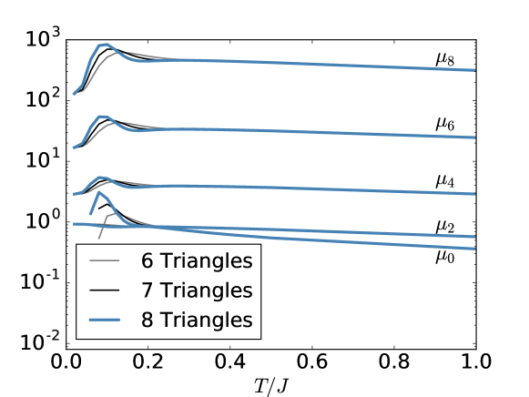
Figure 1: Frequency moments of the spectral function $\hat{K_{o}}$ for Oxygen NMR. The 6th, 7th and 8th order calculations are shown. Note that they converge quite well down to a temperature of $0.2$ J.

Reconstructing a distribution from its moments is, in general, an ill-posed problem . One scheme is the method of maximum entropy numerical-recipes , but this method did not prove to be most useful to us. Instead, we assume a trial functional form $\hat{K_{a}^{t}}$ for $\hat{K}_{a}$, with tunable parameters $a_{1},\cdots,a_{n}$ with $n$ the number of computed moments. We then compute trial moments $\mu_{i}^{t}$ of $\hat{K_{a}^{t}}$. This converts the problem of constructing the best $\hat{K_{a}^{t}}$ into a minimization problem, where we find the $\{a_{i}\}$ that minimizes our cost function $C(\{a_{i}\})$ defined by

$$C(\{a_{i}\})=\sum_{i}\left(\frac{\mu_{i}-\mu_{i}^{t}}{\mu_{i}}\right)^{2}.$$ (12)

Note that, if the fit works well, the minimum of such a function occurs when $\mu_{i}=\mu_{i}^{t}$ for each such $i$, and the value of $C$ is 0.

We discuss two trial functions. First a triple Gaussian $\hat{K_{a}^{G}}$, with one Gaussian centered at $\omega=0$ and the other two symmetrically at a positive and a negative $\omega$ value. This trial function gave NMR results close to Moriya’s Gaussian approximation. However, the cost function $C$ was only on the order of 0.01, implying that it did not reproduce all the moments accurately.

The second is a Lorentzian function of the form

$$\hat{K_{a}^{L}} =\frac{a_{1}}{a_{2}+\omega^{2}}\sum_{s\in\{-1,1\}}\exp\bm{\left(}-\left(\frac{\omega+sa_{3}}{a_{4}}\right)^{a_{5}}\bm{}.$$ (13)

Since we know that all frequency moments are finite, the Lorentzian line-shape was cutoff in a suitable manner. $\hat{K_{a}^{L}}$ had remarkable numerical success, giving values of the cost function $C$ on the order of $10^{-10}$.

We show structure factors obtained from both reconstructions of $\hat{K_{o}}$ in Fig. 2. In our fit for the Lorentzian lineshape, the value of $a_{3}$, for all temperatures studied, was roughly 2. This implies a rapid cutoff of spectral weight for $\omega/J>2$. If we consider a simple Ising model on the kagome lattice, when one spin is flipped, it would change energies of at most 4 bonds, corresponding to a maximum energy difference of $2J$. The Heisenberg model has more complex behavior as a spin-flip can couple the many-body states with arbitrary different energies. Nevertheless, we find that the spectral weights die off rapidly for frequencies larger than $2J$ in our model.

The decay exponent $a_{5}$ was mostly around 1.4 in our fits and always between 1 and 2 as found in spin chains sandvik . Both plots show a peak at frequencies away from zero, but the Lorentzian lineshape shows an additional peak at low frequencies. This low frequency peak is missed by the Gaussian lineshape and Moriya’s Gaussian approximation. This peak may gradually move away from zero as temperature is decreased, in a spin gap system.

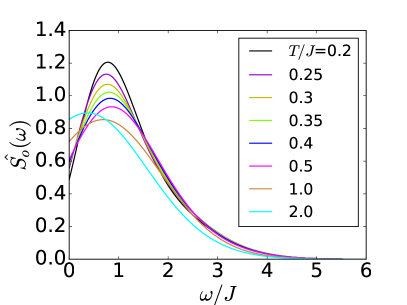
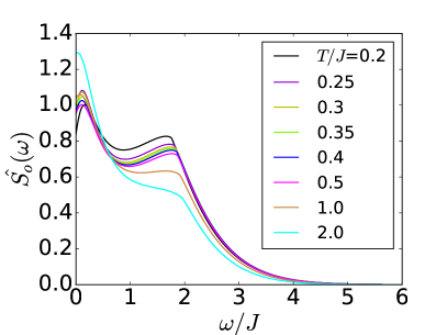
Figure 2: Plots of the frequency dependence of the bond structure factor relevant to oxygen NMR. On the left we have results for $\hat{S}_{o}$ from the Gaussian spectral function $\hat{K_{o}^{G}}$ which is dominated by short time behavior. On the right we have results for $\hat{S}_{o}$ from the Lorentzian spectral function $\hat{K_{o}^{L}}$, which gives a much better fit to the frequency moments.

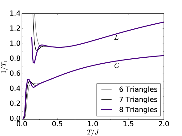
Figure 3: $1/T_{1}$ for the oxygen nucleus from Moriya’s Gaussian approximation and the Lorentzian lineshape obtained from fitting all the frequency moments.

A comparison of the NMR rates calculated by the Lorentzian lineshape and Moriya’s Gaussian approximation is shown in Fig. 3. We see that while the temperature dependence is similar in the two cases, the Gaussian approximation consistently underestimates the rates by up to a factor of 2. One advantage of the Gaussian approximation is that, since it is based on the short time behavior, it can be continued all the way to $T=0$, whereas the more detailed extrapolation clearly breaks down at lower temperatures.

Comparison with experiments: To compare our results with the experimental data we need the hyperfine couplings. For oxygen, the hyperfine Hamiltonian can be written as

$${H}_{hf}=\sum_{m=1,2}\sum_{\alpha=i,j,k}B_{(\alpha)}I^{\alpha}S_{m}^{\alpha},$$ (14)

where $B_{(\alpha)}$ represents the hyperfine coupling through the electron spin polarization induced in the 2s and/or 2p orbitals of the ¹⁷O sites. The sum over $m=$ $1$, $2$ refers to the two equidistant copper spins from the oxygen nucleus. Following the procedure outlined in gelfand , the high temperature limit of $1/T_{1}$, in Moriya’s Gaussian approximation, is given by

$$\frac{1}{T_{1M}}(T=\infty)=\frac{\sqrt{\pi}\{B_{(j)}^{2}+B_{(k)}^{2}\}}{8\hbar J}\frac{4}{\sqrt{3}}.$$ (15)

This sets the overall normalization for the rates in terms of the hyperfine couplings and exchange constant $J$.

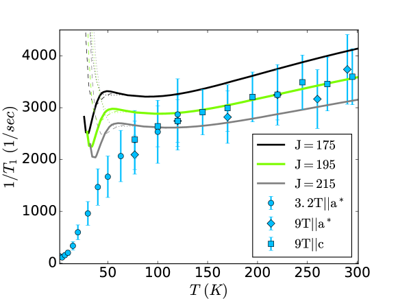
Figure 4: $1/T_{1}$ for the oxygen nucleus as a function of temperature computed using the Lorentzian lineshape and our calculated frequency moments compared with the experimental data on Herbertsmithite. The solid lines are the 8th order, dashed lines 7th order and dotted lines 6th order calculations. The lower orders can only be seen when they differ from the 8th order. The experimental data shows some dependence on the orientation of the magnetic field (for details see FuScience and supplementary materials), we rescaled the data for the field along $a$ to have the same value as the field along c at $T=120$ K. Three different values for the exchange parameter $J$ are shown. The best fit gives $J=195$ K.

Using the standard notation for the hyperfine coupling in the NMR literature, ImaiLadder ; ItohCuGeO3 let $\widetilde{B}_{(\alpha)}=B_{(\alpha)}/g\gamma_{n}\hbar$. From the measurements of the spin susceptibility Imai2011 and the Knight shift FuScience , we obtain the transferred hyperfine coupling tensor for oxygen to be $(\widetilde{B}_{(a)},\widetilde{B}_{(a^{*})},\widetilde{B}_{(c)})=(33,43,36)$ kOe. This now leaves the exchange constant $J$ as the only free parameter in our calculations.

The comparison is shown in Fig. 4. We see a very good agreement between experiment and theory with $J$ in the range $195\pm 20$ K. These values for $J$ are in agreement with other experiments klhm-e and with ab initio calculations valenti . The convergence of our calculation breaks down at low temperatures just as the rates show evidence for a sharp drop with temperature.

Discussions and Conclusions: We have used the Numerical Linked Cluster method to calculate the Nuclear Magnetic Relaxation rates in kagome antiferromagnets in Moriya’s Gaussian approximation and beyond. While the Gaussian approximation gives a qualitatively correct behavior of the temperature dependence of the rates including a spin-gap like feature at low temperatures, it underestimates the magnitude of the relaxation rates by up to a factor of two even at temperatures above the exchange energy scale $J$. The use of higher moments fixes the discrepency at high temperatures giving very good quantitative agreement with the experimental data with a value of $J=195\pm 20$ K. This shows that despite the presence of antisite disorder, the Heisenberg model provides a good quantitative model for intrinsic spin dynamics of Kagome planes in Herbertsmithite as obtained in the NMR measurements.

However, the convergence of our calculations with multiple frequency moments clearly breaks down just as the rates appear to decrease sharply with temperature. Thus, we are unable to theoretically address the existence of a spin-gap in the system. The breakdown of NLC implies the existence of longer-range dynamic correlations in the system in contrast to very short-range static correlations. This causes individual moments to not converge within NLC. There is also need for more moments to capture the more complex frequency dependence expected at low temperatures. We believe that physically this breakdown marks the onset of a coherent regime, where the high energy modes, which contribute an increasing amount to the moments, can now propagate coherently over longer distances. Such a physics is implicit in the sharp spectral features in the Brillouin Zone seen in neutron scattering experiments neutron and the calculations based on Z₂ spin liquids sachdev .

One intriguing feature of our calculations is that the rates show a small peak and then a sharp downturn towards zero. It is seen in Moriya’s Gaussian approximation but also obtained in the extrapolation with multiple moments. Unfortunately, our convergence breaks down around this temperature. Thus, more theoretical studies, perhaps based on $Z_{2}$ quantum spin-liquids sachdev ; oleg , are needed to see if such a behavior is real or an artifact of these computational methods. We note that such a peak is not seen in the experimental data.

We also find that the spectral functions are well described by a Lorentzian lineshape at low frequencies. This implies that the kagome-lattice Heisenberg model has much larger low frequency spectral weights at finite $T$ than would be expected just from the short time behavior. When available, it would be interesting to compare our spectral weights with neutron scattering measurements deVries in the temperature range between $50$ and $300$ K, where our calculations are most reliable. Finite temperature DMRG methods, using minimally entangled thermal states mets may allow for the calculation of spectral functions at still lower temperatures.

In a system like Herbertsmithite, where much of the low temperature and low frequency bulk behavior may be affected by impurities, quantitative understanding of the local probes such as NMR is essential to elucidate the nature of the exciting quantum spin-liquid phase and our calculations represent a step in that direction.

Acknowledgements: This work is supported in part by the US National Science Foundation grant DMR-1306048 (NS and RRPS) and NSERC and CIFAR in Canada (TI).

References

- (1) L. Balents, Nature 464, 199-208 (2010).
- (2) T. Imai and Y. Lee, Physics Today, 69, 30 (2016).
- (3) S. Yan, D. A. Huse and S. R. White, Science 332, 1173 (2011); S. Depenbrock, I. P. McCulloch and U. Schollwock, Phys. Rev. Lett. 109, 067201 (2012); H. C. Jiang, Z. H. Wang and L. Balents, Nat. Phys. 8, 902 (2012);
- (4) P. Lecheminant, B. Bernu, C. Lhuillier, L. Pierre and P. Sindzingre, Phys. Rev. B 56, 2521 (1997).
- (5) C. Waldtmann, et al Eur. Phys. J. B 2, 501 (1998).
- (6) F. Mila, Phys. Rev. Lett. 81, 2356-2359 (1998).
- (7) F. Wang and A. Vishwanath, Phys. Rev. B 74, 174423 (2006).
- (8) N. Elstner and A. P. Young Phys. Rev. B 50, 6871 (1994).
- (9) J. B. Marston and C. Zeng, J. Appl. Phys. 69, 5962 (1991); A. V. Syromyatnikov and S. V. Maleyev, Phys. Rev. B66, 132408 (2002); P. Nikolic and T. Senthil, Phys. Rev. B 68, 214415 (2003); R. Budnik and A. Auerbach, Phys. Rev. Lett. 93, 187205 (2004); R. R. P. Singh and D. A. Huse, Phys. Rev. B 76, 180407 (2007).
- (10) Y. Ran, M. Hermele, P. A. Lee, and X. -G. Wen, Phys. Rev. Lett. 98, 117205 (2007).
- (11) R. R. P. Singh and D. A. Huse, Phys. Rev. Lett. 68, 1766 (1992).
- (12) Y. Iqbal, D. Poilblanc and F. Becca, Phys. Rev. B 91, 020402(R) (2015); Phys. Rev. B 89, 020407 (2014); Y. Iqbal, F. Becca, S. Sorella, D. Poilblanc Phys. Rev. B 87, 060405(R) (2013).
- (13) H. Nakano and T. Sakai, J. Phys. Soc. Jpn 80, 053704 (2011).
- (14) J. S. Helton et al, Phys. Rev. Lett. 98, 107204 (2007); P. Mendels et al Phys. Rev. Lett. 98, 077204 (2007); A. Zorko et al Phys. Rev. Lett. 101, 026405 (2008); T. Han, S. Chu, Y. S. Lee, Phys. Rev. Lett. 108, 157202 (2012).
- (15) T. Imai et al, Phys. Rev. Lett. 100, 077203 (2008);
- (16) M. Rigol and R. R. P. Singh, Phys. Rev. Lett. 98, 207204 (2007).
- (17) G. Misguich and P. Sindzingre, Eur. Phys. J. B 59, 305 (2007).
- (18) T. H. Han et al, Nature 492, 406 (2012).
- (19) M. Punk, D. Chowdhury, and S. Sachdev, Nature Physics 10, 289-293 (2014).
- (20) M. Fu et al., Science 350, 655 (2015)
- (21) J. S. Helton et al, Phys. Rev. Lett. 104, 147201 (2010).
- (22) H. Kawamura, K. Watanabe, T. Shimokawa, J. Phys. Soc. Jpn. 83, 103704 (2014).
- (23) R. R. P. Singh, Phys. Rev. Lett. 104, 177203 (2010).
- (24) T. Moriya, Prog. Theor. Phys. 16, 23 (1956)
- (25) T. Imai et al., Phys. Rev. Lett. 70, 1002 (1993)
- (26) M. P. Gelfand and R. R. P. Singh, Phys. Rev. B 47, 14413 (1993); R. R. P. Singh and M. P. Gelfand, Phys. Rev. B 42, 996 (1990).
- (27) M. Rigol, T. Bryant, R. R. P. Singh, Phys. Rev. E 75, 061118 (2007); ibid. Phys. Rev. Lett. 97, 187202 (2006).
- (28) T. Imai et al., Phys. Rev. B 84, 020411 (2011)
- (29) W. H. Press, S. A. Teukolsky, W. T. Vetterling and B. P. Flannery, Numerical Recipes, Cambridge University Press, Cambridge (1986).
- (30) T. Imai et al., Phys. Rev. Lett. 81, 220 (1998)
- (31) M. Itoh et al., Physica C 263, 486 (1996)
- (32) H. O. Jeschke, F. Salvat-Pujol, and R. Valenti, Phys. Rev. B 88, 075106 (2013).
- (33) M. A. de Vries et al, Phys. Rev. Lett. 103, 237201 (2009).
- (34) O. A. Starykh, R. R. P. Singh, and A. W. Sandvik, Phys. Rev. Lett. 78, 539 (1997); O. A. Starykh, A. W. Sandvik, and R. R. P. Singh, Phys. Rev. B 55, 14953 (1997).
- (35) Z. Hao and O. Tchernyshyov, Phys. Rev. B 87, 214404 (2013); Y. Wan and O. Tchernyshyov Phys. Rev. B 87, 104408 (2013);
- (36) L. C. Hebel and C. P. Slichter Phys. Rev. 113, 1504 (1959).
- (37) S. R. White, Phys. Rev. Lett. 102, 190601 (2009); E. M. Stoudenmire and S. R. White, New J. Phys. 12 055026 (2010).