Detecting topological superconductivity using low-frequency doubled Shapiro steps

Abstract

The fractional Josephson effect has been observed in many instances as a signature of a topological superconducting state containing zero-energy Majorana modes. We present a nontopological scenario which can produce a fractional Josephson effect generically in semiconductor-based Josephson junctions, namely, a resonant impurity bound state weakly coupled to a highly transparent channel. We show that the fractional ac Josephson effect can be generated by the Landau-Zener processes which flip the electron occupancy of the impurity bound state. The Josephson effect signature for Majorana modes become distinct from this nontopological scenario only at low frequency. We prove that a variant of the fractional ac Josephson effect, namely, the low-frequency doubled Shapiro steps, can provide a more reliable signature of the topological superconducting state.

Superconductors supporting Majorana zero modes (MZMs)Salomaa and Volovik (1988); Read and Green (2000); Kitaev (2001); Sengupta et al. (2001) at defects provide one of the simplest examples of topological superconductors (TSs) Schnyder et al. (2008); Kitaev (2009). In fact, a number of proposals Fu and Kane (2008); Sau et al. (2010a, b); Jason Alicea (2010); Roman M. Lutchyn, Jay D. Sau, and S. Das Sarma. (2010); Yuval Oreg, Gil Refael, and Felix von Oppen. (2010) to realize such MZMs have met with considerable success V. Mourik, K. Zuo, S. M. Frolov, S. R. Plissard, E. P. A. M. Bakkers and L. P. Kouwenhoven. (2012); M. T. Deng, C. L. Yu, G. Y. Huang, M. Larsson, P. Caroff, and H. Q. Xu. (2012); Anindya Das, Yuval Ronen, Yonatan Most, Yuval Oreg, Moty Heiblum and Hadas Shtrikman. (2012); Churchill et al. (2013); Finck et al. (2013); Lee et al. (2014). Such systems containing MZMs are particularly interesting Alicea (2012); Beenakker (2013); Leijnse and Flensberg (2012); Stanescu and Tewari (2013); Elliott and Franz (2015); Sarma et al. (2015); Beenakker and Kouwenhoven (2016) because of the topologically degenerate Hilbert space and non-Abelian statistics associated with them that make such MZMs useful for realizing topological quantum computation Nayak et al. (2008). While preliminary evidence for MZMs in the form of a zero-bias conductance peak have already been observed V. Mourik, K. Zuo, S. M. Frolov, S. R. Plissard, E. P. A. M. Bakkers and L. P. Kouwenhoven. (2012); M. T. Deng, C. L. Yu, G. Y. Huang, M. Larsson, P. Caroff, and H. Q. Xu. (2012); Anindya Das, Yuval Ronen, Yonatan Most, Yuval Oreg, Moty Heiblum and Hadas Shtrikman. (2012); Finck et al. (2013); Nadj-Perge et al. (2014); He et al. (2016); Sun et al. (2016); Zhang et al. (2016); Churchill et al. (2013); Albrecht et al. (2016); Lee et al. (2014), confirmatory signatures of the topological nature of MZMs are still lacking.

The zero-bias conductance peak provides evidence for the existence of zero-energy end modes which can arise not only from TSs but also from a variety of nontopological features associated with the details of the end of the system Liu ; Bagrets ; Sau ; Brouwer . In contrast, the topological invariant of a TS, being a bulk property, is not affected by the details of the potential at the end. The topological invariant of a one-dimensional TS can be determined from the change in the fermion parity of the Josephson junction (JJ) Kitaev (2001). Specifically, the fermion parity of a topological JJ changes when the superconducting phase of the left superconductor $\phi$ of the JJ winds adiabatically by $\delta\phi=2\pi$  Read and Green (2000); Kitaev (2001). Such a change in fermion parity of the JJ may be detected from the resulting $4\pi$-periodic component in the current-phase relation of the topological JJ Kitaev (2001); Kwon et al. (2004). This is referred to as the fractional Josephson effect and can be detected using the fractional ac Josephson effect (FAJE).

The FAJE involves applying a finite dc voltage $V$ across the junction so that the superconducting phase across the junction varies in time as $\phi(t)=\Omega_{J}t$ Tinkham (2004). Here, $\Omega_{J}=V$ is the Josephson frequency, where we have set $\hbar=1$ and the charge of the Cooper pair $2e=1$. The $4\pi$-periodic current-phase relation characteristic of a topological JJ results in a current that has a component at half the Josephson frequency, i.e., at $\omega=\Omega_{J}/2$ instead of $\omega=\Omega_{J}$ characteristic of conventional JJs Kitaev (2001); Kwon et al. (2004); Fu and Kane (2009); Roman M. Lutchyn, Jay D. Sau, and S. Das Sarma. (2010); Yuval Oreg, Gil Refael, and Felix von Oppen. (2010); Zocher et al. (2012). In principle, the resulting ac current may be detected by a measurement of the radiation emitted from the junction  Billangeon et al. (2007); Deacon et al. (2016). Alternatively, the fractional Josephson effect can also be detected by measuring the size of the voltage steps, known as Shapiro steps Rokhinson et al. (2012); Wiedenmann et al. (2016). For topological JJs, these voltage steps have been numerically found to be $\delta V=2\Omega_{J}$, which is double the voltage steps for the conventional JJs Domínguez et al. (2012); yuri .

Interestingly, evidence for both the FAJE Deacon et al. (2016) and doubled Shapiro steps Rokhinson et al. (2012); Pribiag et al. (2015); Wiedenmann et al. (2016) have been seen in TSs that are expected to support MZMs. However, there is evidence that such signatures might appear in nontopological systems as well. For example, both the signatures seem to also appear in the TS experiments when the devices are not in the topological parameter regime Wiedenmann et al. (2016); Pribiag et al. (2015); Deacon et al. (2016); Sup (a). One possible spurious source of FAJE is the period-doubling transition seen in certain JJ systems Wiesenfeld and McNamara (1985). In addition, the FAJE and doubled Shapiro steps are known (both experimentally Billangeon et al. (2007) and theoretically Sau et al. (2012); Sothmann et al. (2013)) to arise from Landau-Zener (LZ) processes in certain ranges of frequency. Avoiding such LZ processes might require particularly low frequencies in low-noise systems with multiple MZMs Sticlet et al. (2013). While the LZ process is known to potentially lead to FAJE Billangeon et al. (2007); Sau et al. (2012), there have not been any generic nontopological scenarios presented in the literature so far.

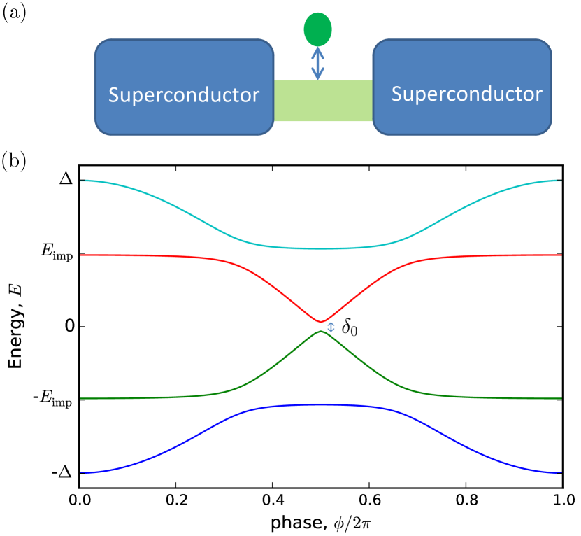
Figure 1: (Color online) (a) JJ configuration showing FAJE consists of a high transparency channel connecting two superconductors. The channel is tunnel coupled to an impurity bound state (shown as a disk adjoining wire). (b) Computed Andreev bound state spectrum for the setup in (a) shows a weakly avoided crossing at $E=0$ and a gap to higher-energy states generated by a larger avoided crossing with the flat impurity bound state. The weakly avoided crossing can lead to an FAJE at finite voltages.

In this Rapid Communication, we start by discussing a generic model of a resonant impurity coupled to a JJ [shown in Fig. 1(a)], which has a weakly avoided crossing in the energy spectrum as a function of phase [see Fig. 1(b)]. The present scenario requires only the coexistence of a highly transparent channel in a JJ [as seen in recent measurements of ABS spectra Chang et al. (2013)] and a weakly coupled impurity bound state. Such a coexistence can be found in a multichannel semiconductor-based JJ with a spatially varying density, as is the case of all of the recent experiments Wiedenmann et al. (2016); Deacon et al. (2016); Pribiag et al. (2015); Rokhinson et al. (2012). We use a scattering-matrix approach to show that this relatively generic situation can lead to an FAJE over a frequency range of a factor of a few even in the absence of any TS. In order to distinguish between this nontopological scenario from TS, it is important to be able to go to ultralow MHz frequencies in the FAJE measurements. Shapiro steps provide the setup where such a large range of frequencies spanning three orders of magnitudes (MHz–GHz) are possible Hebboul et al. (1990). In the second part of this Rapid Communication, we provide a rigorous framework connecting Shapiro steps to TS where we show that the low-frequency doubled Shapiro steps are guaranteed to appear in the overdamped driven measurements of topological JJs.

Let us first understand how an FAJE can occur in a nontopological setup such as the setup in Fig. 1(a). For simplicity, we consider the superconductors to be $s$ wave with a highly transparent normal channel in between together with a subgap impurity bound state. The highly transparent channel supports Andreev bound states (ABSs) in the junction that approach zero energy [see Fig. 1(b)] when the phase $\phi$ crosses $\phi=\pi$ Beenakker (1991). Applying a finite voltage $V$ across the junction causes the superconducting phase $\phi$ to vary in time as $\phi(t)=Vt$. This leads to the possibility of LZ processes exciting Cooper pairs across the superconducting gap. In general, these Cooper pairs are transported across the entire superconducting gap via multiple Andreev reflections Averin and Bardas (1995); Klapwijk et al. (1982), ultimately leading to a dissipative but otherwise conventional ac Josephson effect Averin and Bardas (1995). This situation is modified when the junction is tunnel coupled to impurity bound states. As shown in Fig. 1(b), the ABS spectrum of the JJ varies with phase $\phi$ where it crosses the relatively flat impurity bound state with energy $E_{\mathrm{imp}}$ at pairs of points. At such crossings, the junction exchanges a Cooper pair with the flat impurity state. When $\phi=\pi$, the ABS loses a Cooper pair to the condensate through a LZ process across the zero-energy gap $\delta_{0}$. As the ABS energy approaches the second avoided crossing with the impurity bound state at energy $E_{\mathrm{imp}}$, the ABS restores its Cooper pair at the expense of leaving the impurity bound state empty. Thus, the impurity bound state electron occupancy is flipped via the LZ process as the phase varies over a period of $\phi=0$ to $\phi=2\pi$ which is restored during the next $2\pi$ cycle. Therefore, while the spectrum of the junction is $2\pi$ periodic, the occupation of the impurity bound state is $4\pi$ periodic. Since the total energy $E$ which includes the spectrum and occupation of the ABS and impurity bound states determines the supercurrent $I(\phi)$ by $I(\phi)\sim\partial_{\phi}E(\phi)$, $I(\phi)$ would also be $4\pi$ periodic with the phase $\phi$. This manifests as a peak in the radiation spectrum from the current at a frequency of $\omega=\Omega_{J}/2$ instead of the usual Josephson frequency $\omega=\Omega_{J}$ peak.

While the qualitative argument above suggests the possibility of an FAJE occurring in nontopological semiconductor systems, it assumes the zero-energy LZ processes to be perfect and all other LZ processes to be completely avoided. In the following, we perform a completely unbiased quantitative analysis of the FAJE for the JJ shown in Fig. 1. To begin with, we note that at any finite voltage $V$, the occupation of an ABS fluctuates due to excitations out of the bulk gap (via multiple Andreev reflections). The quasiparticle fluctuations ensure that the system equilibrates to the grand canonical ensemble (with no conserved fermion parity) such that the expectation value of the current is $2\pi$ periodic as in the conventional system  Bloch (1970). Thus, strictly speaking, the FAJE at any finite voltage is subject to random fluctuations and can only appear in the noise spectrum of the current Badiane et al. (2011, 2013). To assess the range of voltages over which the JJ shown in Fig. 1(a) exhibits an FAJE, we compute the noise spectrum of the current

$$P(\omega)=\int d\tau e^{i\omega\tau}[\langle{I(t)I(t+\tau)}\rangle-\langle{I(t)}\rangle\langle{I(t+\tau)}\rangle],$$ (1)

where $\langle{\cdots}\rangle$ denotes the averaging over time $t$. The current Averin and Bardas (1995) and its noise spectrum Badiane et al. (2011, 2013) can be computed by considering the scattering of quasiparticles between the superconducting leads, which are at different voltages. This approach has the advantage of including the contribution of not only the low-energy ABSs but also all bound and scattering states in the junction. We have expanded this formalism to general superconductor-normal-superconductor junctions Sup (b). Our general framework can be easily implemented with Kwant Groth et al. (2014) which supplies the normal-superconductor scattering matrices. The resulting power spectrum $P(\omega)$ is plotted against the frequency scaled by the Josephson frequency, i.e., $\omega/\Omega_{J}$ in Fig. 2 for various voltages for the system depicted in Fig. 1(a) with the spectrum shown in Fig. 1(b). The power spectrum at high voltages is quite broad, which becomes narrower at lower frequency and develops peaks in the vicinity of $\omega/\Omega_{J}=1/2$ before splitting off to different values. The high-frequency spectrum is also several orders smaller in magnitude, which is expected in the adiabatic limit when fluctuations in the ABS occupation are small. While some of the peaks appear to move away from the ideal fractional value and come back, this might be difficult to resolve at a high level of broadening arising from nearby energy states and circuit-noise induced broadening.

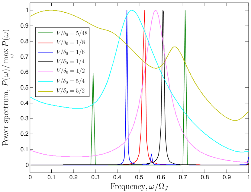
Figure 2: (Color online) Power radiated $P(\omega)$ as a function of frequency $\omega/\Omega_{J}$ for different ratios of the applied voltage $V$ relative to the zero-energy gap $\delta_{0}$. The power spectrum $P(\omega)$ shows a fractional ac Josephson peak at $\omega=\Omega_{J}/2$ for a range of values of $V/\delta_{0}$. The peak broadens out at higher voltages and shifts towards a more conventional peak at $\omega=\Omega_{J}$ at lower frequency (while becoming smaller). $P(\omega)$ has been rescaled so that all peaks are clearly visible.

The spurious FAJE peaks in Fig. 2 resulting from the LZ mechanism appear over a frequency range narrower compared to the parametrically large frequency range (i.e., $\Gamma,\delta\leq\omega\leq\Delta$) of the FAJE in a high-quality TS Pikulin and Nazarov (2012); San-Jose et al. (2012); Badiane et al. (2011, 2013). Here, $\Delta$ is the induced superconducting gap, which is a relatively large frequency ($\sim$ GHz), and $\Gamma$ and $\delta$ are respectively the quasiparticle poisoning rate and the MZM overlap that become vanishingly small ($\lesssim$ MHz) in high-quality TSs.

It is clear from Fig. 2 that distinguishing a bona fide TS from an LZ-type mechanism induced by resonant bound states requires low-frequency ($\lesssim 50$ MHz) measurements of high-quality TS devices with $\Delta\gg\delta,\Gamma$. The FAJE which involves measuring small oscillating currents is difficult to perform for low frequencies because such small oscillating currents are typically measured using on-chip detectors Billangeon et al. (2007); Kouwenhoven03 that are suited to measure relatively high frequencies ($\sim$ GHz). On the other hand, the Shapiro step Tinkham (2004), which is a variant of the FAJE, has been demonstrated over a large range of frequencies from several MHz to GHz Hebboul et al. (1990). While this makes the Shapiro step promising for the detection of TSs, a rigorous proof establishing the doubled Shapiro step as a signature of TS is still missing from the literature. Below, we demonstrate analytically that the low-frequency doubled Shapiro steps can be used as a reliable signature of TS.

We begin by considering the Shapiro step experiment where a JJ shunted with a resistance $R$ is biased with a time-varying current $I_{\mathrm{bias}}(t)=I_{\mathrm{dc}}+I_{\mathrm{ac}}\cos{(\Omega_{J}t)}$, with $I_{\mathrm{dc}}$ and $I_{\mathrm{ac}}$ being dc and ac bias currents, respectively. For the following analysis, we make a key assumption that we are working in the limit of low-frequency $\Omega_{J}$ so that the Josephson current $I_{J}(\phi(t))$ can be taken to be in equilibrium, apart from the conserved local fermion parity. The assumption of being at sufficiently low frequency can only be justified by studying the Shapiro steps over a few orders of magnitude in frequency (from $\Delta\sim$ GHz to $\delta,\Gamma\sim$ MHz). Using this assumption and the result of Bloch Bloch (1970), we can establish that $I_{J}(\phi)$ for any nontopological system must be $2\pi$ periodic and thus rule out any nontopological FAJE such as those from the LZ mechanism.

Furthermore, assuming that the shunt resistance $R$ is small enough to allow the JJ to be overdamped, the equation of motion for $\phi(t)$ for the resistively shunted JJ takes the standard form Tinkham (2004)

$$\frac{d\phi}{dt}=R[I_{\mathrm{bias}}(t)-I_{J}(\phi(t))].$$ (2)

For illustration purposes, we will choose a simple case of $I_{J}(\phi)=I_{0}\cos{(2\pi\phi)}+I_{\mathrm{top}}\cos{(\pi\phi)}$, where $I_{0}$ and $I_{\mathrm{top}}$ are the 2$\pi$- and 4$\pi$-periodic components of the critical current of the adiabatic current-phase relation, respectively. However, our results generally hold and do not depend on this parameter choice as is proven by the analytic arguments in Ref. Sup (c). The dc voltage $V$ across the JJ is calculated by considering the average change of the phase

$$V=\lim_{t\rightarrow\infty}\frac{\phi(t)-\phi(0)}{t},$$ (3)

where the limit is computed by choosing a sufficiently long simulation time for Eq. 2.

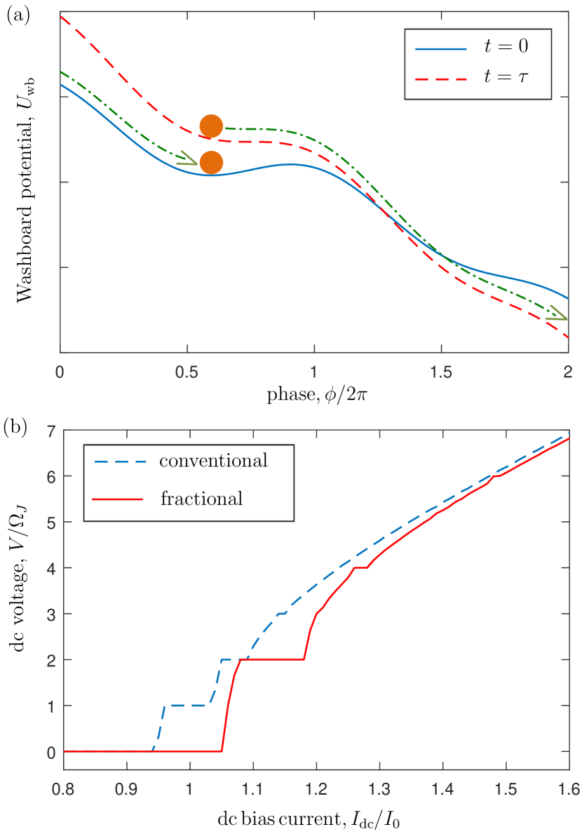
Figure 3: (Color online) (a) Schematic of a phase particle (orange disk) on a tilted washboard potential that describes the phase dynamics in an overdamped JJ. As the bias current increases from $t=0$ to $t=\tau$, the phase particle is released from the local minimum and traverses the trajectory along the green dashed-dotted arrow, and stops when the current bias is back to its value at $t=0$ and the phase particle has traveled by $4\pi$ (for the TS case shown here). This corresponds to a voltage step of 2$\Omega_{J}$. (b) Shapiro step calculated numerically for a putative fractional Josephson system shows doubled Shapiro steps (see also Ref. Domínguez et al., 2012) as opposed to a conventional system with all integer Shapiro steps for an overdamped JJ. Here, $I_{\mathrm{ac}}=0.1I_{0}$, $R=25$, $I_{\mathrm{top}}=0.15I_{0}$ (for fractional), and $I_{\mathrm{top}}=0$ (for conventional).

We will now show that overdamped JJs constructed out of TSs are generically characterized by a doubled Shapiro step in the strongly overdamped and low-frequency limit (i.e., $\Omega_{J}/I_{J}R\ll 1$). The dynamics of $\phi(t)$ described by Eq. 2 can be understood simply by an analogy of a “phase particle” rolling down a washboard potential according to the equation $\dot{\phi}(t)=-\partial_{\phi}U_{\mathrm{wb}}(\phi,t)$, where the washboard potential is written as $U_{\mathrm{wb}}=-R[I_{\mathrm{bias}}(t)\phi-\int d\phi I_{J}(\phi)]$. As seen in Fig. 3(a), because of the ac drive, the potential $U_{\mathrm{wb}}(\phi,t)$ varies in time with local minima at each cycle when $\phi(t)=\phi_{0}$ such that

$$I_{\mathrm{bias}}(t)-I_{J}(\phi_{0})=0.$$ (4)

In the adiabatic limit (i.e., $\Omega_{J}/I_{J}R\ll 1$), one can show that the phase particle approaches the minimum of the washboard potential exponentially in time once every period of the drive. This leads to a well-defined voltage that appears as a sharp plateau in the Shapiro steps Sup (c).

Let us for now assume that Sup (c) the phase particle approaches a minimum of $U_{\mathrm{wb}}$ during the time interval when such exists. In the conventional case of a $2\pi$-periodic function $I_{J}$, this can occur once in a $2\pi$ period provided the critical current $I_{J,\mathrm{max}}>(I_{\mathrm{dc}}-I_{\mathrm{ac}})$. This will certainly occur if $I_{\mathrm{dc}}$ is small enough. In addition, if $I_{\mathrm{dc}}>(I_{J,\mathrm{max}}-I_{\mathrm{ac}})$, then there will be a range of time when $U_{\mathrm{wb}}$ has no minimum and the adiabatic solution breaks down. In this case, $\phi(t)$ will wind by a multiple of $2\pi$ and collapse to $\phi_{0}$ after a winding of $2\pi n$. The result is that an integer voltage appears across the JJ. In the case of a topological JJ, the current-phase relation $I_{J}(\phi)$ has a $4\pi$-periodic component and one can define two critical currents $I_{J,\mathrm{max}}$ and $I_{J,\mathrm{max}}^{\prime}$, one associated with the range $\phi\in[4n\pi,(4n+2)\pi]$ and the other in the range $\phi\in[(4n-2)\pi,4n\pi]$. In our simple model $I_{J,\mathrm{max}},I_{J,\mathrm{max}}^{\prime}=I_{0}\pm I_{\mathrm{top}}$. As in the conventional case, the dc bias current must satisfy $I_{\mathrm{dc}}>(I_{J,\mathrm{max}}-I_{\mathrm{ac}})$ (assuming $I_{J,\mathrm{max}}>I_{J,\mathrm{max}}^{\prime}$) to exit the zero-voltage state even in the TS case. On the other hand, if $2I_{\mathrm{ac}}<(I_{J,\mathrm{max}}-I_{J,\mathrm{max}}^{\prime})$, then $I_{\mathrm{dc}}>I_{J,\mathrm{max}}^{\prime}+I_{\mathrm{ac}}$ so that the phase particle cannot stop at one half of the minima. This leads to a doubled voltage step for the topological case, as seen from the numerical solution of Eq. 2 [see Fig. 3(b)].

In summary, we have shown that while the FAJE can be viewed as a smoking gun for the TS with MZMs, a detailed study of the frequency dependence of the FAJE is necessary before concluding a system to have realized the TS. We have shown this by considering a generic model of a high transparency channel in a JJ coupled weakly to a resonant impurity. We find this model to show an FAJE quite generically in semiconductor-based JJs, similar to the TS case with MZMs. Nevertheless, TSs are expected to show FAJE over a parameterically larger range of frequency. We argue that the current-phase relation over such a range of frequency, particularly at the low-frequency end, is better studied by considering the Shapiro step experiment. We present a way of understanding the Shapiro step experiment in terms of the tilted washboard potential that guarantees that the necessary and sufficient condition for the existence of doubled Shapiro steps in the low-frequency limit is that the JJ is formed from a TS. Thus, low-frequency Shapiro steps which have been demonstrated in conventional systems can serve as a smoking gun for MZMs.

This work is supported by Microsoft Station Q, Sloan Research Fellowship, NSF-DMR-1555135 (CAREER), and JQI-NSF-PFC. We acknowledge enlightening discussions with Anton Akhmerov, Julia Meyer, Leo Kouwenhoven, Attila Geresdi, Yuli Nazarov, Chang-Yu Hou, Sergey Frolov, Ramon Aguado, and Roman Lutchyn in the course of this work. J.D.S. is grateful to the Aspen Center for Physics where part of this work was completed.

Supplemental Material for “Detecting topological superconductivity using low-frequency doubled Shapiro steps”

I Calculation of the power spectrum for the fractional ac Josephson effect

The current noise can be calculated using the scattering matrix approach similar to Refs. Badiane et al. (2011, 2013). Below we discuss a generalization of this approach that allows us to calculate the noise numerically in the general case. The scattering matrix is described in terms of current amplitudes $J^{\rho}_{\ell}$ where $\rho=\pm$ represents the left and right movers, $\ell=L,R$ denotes the left and right superconductors and $\ell=NL,NR$ are the left- and right-half of the normal intervening region in between the two superconductors. This region is infinitesimally small and only there to allow computation of the scattering matrices $S_{L}$ and $S_{R}$ of the left and right superconductors. In terms of these amplitudes, the scattering matrix equations at the interfaces $L\rightarrow NL$, $NL\rightarrow NR$ and $NR\rightarrow R$ are written as

$$\left(\begin{array}[]{c}\mathcal{J}_{L}^{-,\gamma}(E_{n})\\ \mathcal{J}_{NL}^{+,\gamma}(E_{n})\end{array}\right) =S_{L}(E_{n})\left(\begin{array}[]{c}\mathcal{J}_{L}^{+,\gamma}(E_{n})\delta_{n,0}\delta_{\gamma,L}\\ \mathcal{J}_{NL}^{-,\gamma}(E_{n})\end{array}\right),$$ (S-1e)

$$\left(\begin{array}[]{c}\mathcal{J}_{NL}^{-,\gamma}(E_{n})\\ \mathcal{J}_{NR}^{+,\gamma}(E_{n})\end{array}\right) =\sum_{n^{\prime}}S_{N}(E_{n},E_{n^{\prime}})\left(\begin{array}[]{c}\mathcal{J}_{NL}^{+,\gamma}(E_{n^{\prime}})\\ \mathcal{J}_{NR}^{-,\gamma}(E_{n^{\prime}})\end{array}\right),$$ (S-1j)

$$\left(\begin{array}[]{c}\mathcal{J}_{R}^{+,\gamma}(E_{n})\\ \mathcal{J}_{NR}^{-,\gamma}(E_{n})\end{array}\right) =S_{R}(E_{n})\left(\begin{array}[]{c}\mathcal{J}_{R}^{-,\gamma}(E_{n})\delta_{n,0}\delta_{\gamma,R}\\ \mathcal{J}_{NR}^{+,\gamma}(E_{n})\end{array}\right),$$ (S-1o)

where the superscript $\gamma=L/R$ denotes whether the incoming current is from the left/right superconductor, $E_{n}=E+nV/2$ with $n$ being an integer and $E$ being the incoming quasiparticle energy (as in the main text, we set $2e=1$), and $\mathcal{J}_{\ell}^{\rho,\gamma}=(j_{\ell}^{e,\uparrow,\eta,\gamma},j_{\ell}^{e,\downarrow,\eta,\gamma},j_{\ell}^{h,\uparrow,\eta,\gamma},j_{\ell}^{h,\downarrow,\eta,\gamma})^{\mathrm{T}}$ is the current amplitude in the particle-hole space.

The normal-state transmission is perfect up to a cutoff after which it vanishes completely. The transmission part of the scattering matrix $S_{N}$ is written as

$$t_{N}(E_{n},E_{n^{\prime}})=t_{n}\left[\frac{1+\tau_{z}}{2}\delta_{n,n^{\prime}-1}+\frac{1-\tau_{z}}{2}\delta_{n,n^{\prime}+1}\right],$$ (S-2)

where $\tau_{z}$ is the $z$-Pauli matrix in the particle-hole subspace, $t_{n}=1$ in the transmitting energy interval and zero elsewhere. The reflecting part of $S_{N}$ is analogously defined as

$$r_{N}(E_{n},E_{n^{\prime}})=r_{n}\left[\frac{1+\tau_{z}}{2}\delta_{n,n^{\prime}}+\frac{1-\tau_{z}}{2}\delta_{n+1,n^{\prime}+1}\right],$$ (S-3)

with $r_{n}=\sqrt{1-t_{n}^{2}}$.

The current noise spectrum $P(\omega)$ can be written in terms of the eigenstates of the system as

$$P(\omega)=\sum_{n}|\langle 0|J(\omega)|n\rangle|^{2},$$ (S-4)

where $|0\rangle$ is the state with all incoming quasiparticles from the occupied bands of the superconductors and $|n\rangle=c_{a}c_{b}|0\rangle$ are excited states with negative-energy quasiparticle states $c_{a}$ and $c_{b}$ having been emptied. We will assume that the frequency $\omega$ in the current operator is smaller than the Josephson frequency so that $\omega<V$. Furthermore, we will assume that the chemical potential in the normal region is very large so that we can assume the group velocity to be constant. With these approximations, the current operator $J(\omega)$ (as a matrix in the current amplitude basis) is written as

$$J(\omega)=2\pi\eta_{z}\tau_{z}\delta(E_{n,a}+E_{n^{\prime},b}-\omega),$$ (S-5)

where $\eta_{z}$ is the $z$-Pauli matrix in the left- or right-mover subspace, $E_{n,a}=E_{a}+nV/2$ and $E_{n^{\prime}b}=E_{b}+n^{\prime}V/2$ and $E_{a,b}<0$ are quasiparticle energies. Flipping the energies of one of the states by a particle-hole transformation, we have

$$P(\omega)\sim\int_{E_{a}<0,E_{b}>0} dE_{a}dE_{b}\sum_{\gamma=L/R}|\langle\mathcal{J}^{\gamma}_{NL,a}|\eta_{z}\tau_{z}|\mathcal{J}^{\gamma}_{NL,b}\rangle|^{2}$$

$$\times\sum_{n}\delta(E_{a}-E_{b}+nV/2-\omega),$$ (S-6)

where $\mathcal{J}^{\gamma}_{\mathrm{NL}}=(\mathcal{J}_{\mathrm{NL}}^{+,\gamma},\mathcal{J}_{\mathrm{NL}}^{-,\gamma})^{\mathrm{T}}$.

II Analysis of adiabatic Shapiro step equation

The goal of this section is to develop an analytic understanding of the Shapiro step equation with the end goal of proving the doubling of the Shapiro step period in the topological case. We start with the basic equation of an overdamped Josephson junction, which is justified at sufficiently low frequencies, i.e.,

$$\frac{d\phi}{dt}=R[I_{\mathrm{bias}}(t\Omega_{J})-I_{J}(\phi(t))],$$ (S-7)

where $R$ is the circuit resistance and $\Omega_{J}$ parametrizes the frequency of the drive. We make no assumptions on the specific form of either $I_{\mathrm{bias}}$ or $I_{J}$ other than that they are periodic and the equation $I_{\mathrm{bias}}=I_{J}$ has a solution for most of the time interval (in a sense to be made precise later). In the tilted washboard picture where the washboard potential is defined as

$$\partial_{\phi}U_{\mathrm{wb}}=R[I_{J}(\phi)-I_{\mathrm{bias}}(t\Omega_{J})],$$ (S-8)

this is equivalent to requiring that the washboard potential has local minima for most of the time.

By rescaling time variable as $t\rightarrow tR^{-1}$, we can write the equation of motion [Eq. (S-7)] as

$$\frac{d\phi}{dt}=[I_{\mathrm{bias}}(tR^{-1}\Omega_{J})-I_{J}(\phi(t))].$$ (S-9)

We note that in the adiabatic limit ($\Omega_{J}R\rightarrow 0$), the current bias $I_{\mathrm{bias}}$ in the vicinity of some time $t\sim\tilde{t}$, can be approximated to be quasi-static and Eq. (S-9) can be solved as

$$\int\frac{d\phi}{[I_{\mathrm{bias}}(\tilde{t}R^{-1}\Omega_{J})-I_{J}(\phi)]}=\int dt.$$ (S-10)

Here, we focus on the case where $\tilde{t}$ is such that $I_{\mathrm{bias}}(\tilde{t}R^{-1}\Omega_{J})\neq I_{J}(\phi(\tilde{t}))$ and the phase variable evolves rapidly compared to $I_{\mathrm{bias}}(tR^{-1}\Omega_{J})$. As $\phi$ changes because of the periodic dependence of $I_{J}$, one must approach a minimum of the washboard potential when $[I_{\mathrm{bias}}(\tilde{t}R^{-1}\Omega_{J})-I_{J}(\phi)]\sim 0$ (where the dynamics slows down and the integral on the LHS diverges). There are two relevant time intervals: (i) where $I_{\mathrm{bias}}(tR^{-1}\Omega_{J})=I_{J}(\phi)$ has a solution $\phi=\phi_{0}(t)$ and (ii) where there is no such solution (or local minimum of $U_{\mathrm{wb}}$).

Before analyzing region (i), which will be the focus of our analysis, let us first show that the time range (ii) is small. Scaling $t\rightarrow\Omega_{J}^{-1}t$, the equation of motion [Eq. (S-7)] becomes

$$\frac{d\phi}{dt}=(\Omega_{J}^{-1}R)[I_{\mathrm{bias}}(t)-I_{J}(\phi(t))].$$ (S-11)

In the limit $\Omega_{J}^{-1}R\rightarrow\infty$, the phase $\phi$ can change by a period in a parametrically small time. Changes by a large number of periods would correspond to a large phase. This would correspond to high Shapiro steps as a function of the bias dc current. Therefore, we assume that the dc part of $I_{\mathrm{bias}}$ is small enough past the first Shapiro step, so that the time range (ii) is small. This is the assumption referred to below Eq. S-7.

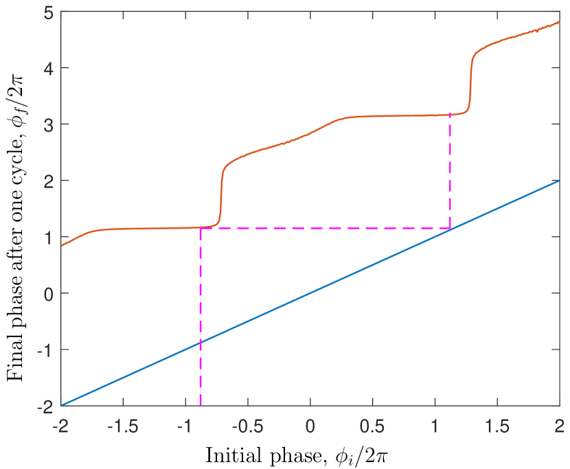
Supplementary Figure S1: (Color online) Poincare map for the dynamics of Eq. S-7 showing the resulting phase $\phi_{f}$ after one period given the initial phase $\phi_{i}$. The long-time periodic dynamics can be computed from the Poincare map. As discussed in the main text, the Poincare map shows doubled steps that correspond to the doubled Shapiro step seen numerically in Fig. 3.

Under this assumption, the dynamics in region (i) spans most of the time. However, based on a similar argument in the previous paragraph, we can argue that the phase dynamics is fast when $I_{J}(\phi)$ is significantly different from $I_{\mathrm{bias}}(t)$. Defining $\phi_{0}(t)$ in the region (i) so that

$$I_{J}(\phi_{0}(t))=I_{\mathrm{bias}}(t),$$ (S-12)

we can assume that $\phi(t)$ rapidly evolves until $\phi(t)\sim\phi_{0}(t)$ (i.e., the phase variable approaches a local extremum) where it slows down. However, the dynamics of the phase variable in this region can be described by linearization by defining

$$\delta\phi=\phi-\phi_{0},$$ (S-13)

whose dynamics is given by the equation

$$\dot{\delta\phi}+\Omega_{J}\dot{\phi}_{0}=-RI_{J}^{\prime}(\phi_{0})\delta\phi.$$ (S-14)

The solution of this equation is written as

$$\delta\phi(t)=e^{-\Lambda(t)}\delta\phi(0)-\Omega_{J}\int dt^{\prime}e^{-(\Lambda(t)-\Lambda(t^{\prime}))}\dot{\phi}_{0}(t^{\prime}),$$ (S-15)

where

$$\Lambda(t)=\frac{R}{\Omega_{J}}\int_{0}^{t}dt^{\prime}I_{J}^{\prime}(\phi_{0}(t^{\prime}))$$ (S-16)

is the Lyapunov exponent of the dynamics. Here $t=0$ represents the time when a particular trajectory approaches close to the minimum $\phi_{0}(t)$.

Let us now use the picture above to construct the Poincare map of the periodic dynamics shown in Fig. S1. The Poincare map for a time-periodic system is defined as a function for the phase variable at the end of a period $\phi=\phi_{f}$ in terms of the initial condition $\phi=\phi_{i}$ at the beginning. Given this function, one can construct the long term dynamics of the equation. Based on the previous paragraph, it is convenient to choose the period at the end of the region (i) where $U_{\mathrm{wb}}$ still has a local minimum and the phase particle is converging to the minimum because of the negative Lyapunov exponent. Assuming the Lyapunov exponent is large (i.e., $\Omega_{J}\rightarrow 0$), the trajectories of $\phi(t)$ over almost the entire range of $\phi$ at the initial point of region (i) (which we called $t=0$ before) converge to one of the minima where $\phi\sim\phi_{0}(t)$. There are, however, some small range of ”transition” values of $\phi$ at $t=0$ where the trajectories do not approach a minimum. Apart from this transition region, the rest of the range of $\phi$ at $t=0$ is compressed to an exponentially small range in $\phi_{f}$. A subtle point to note is that the beginning of region (i) is preceeded by a small range of region (ii) over which the Lyapunov exponent contribution $I_{J}^{\prime}$ is not necessarily positive. This region is the key in connecting the initial time where $\phi_{i}$ is set at the beginning of the period to the time $t=0$ which is the beginning of region (i). It is possible, in principle, that the range away from the transition region which is compressed to an exponentially small part of $\phi_{f}$ is generated from an exponentially small part of $\phi_{i}$. However, because the range of time in (ii) is assumed to be parametrically smaller than (i), the amplification in region (ii) from $\phi_{i}$ to $t=0$ is much smaller than the total Lyapunov exponent $e^{-\Lambda(t)}$ accumulated over region (i). Therefore, we expect plateaus in $\phi_{f}$ as a function of the initial condition $\phi_{i}$ as seen in the Poincare map in Fig. S1.

One can determine from the Poincare map in Fig. S1 that the long-term dynamics will be characterized by a stable attractor where the phase changes by an integer multiple of $4\pi$ over each cycle. To see this, we note that for certain values of the dc bias current $I_{\mathrm{dc}}$, the plateau value of the phase $\phi_{f}$ will occur in a range of $\phi_{i}$ where the plateau is stable. This leads to the phase particle returning to the plateau at regular intervals leading to the Shapiro step in Fig. 3(b). The stability of the trajectory can be further understood by considering the Lyapunov exponent around the proposed trajectory $\phi_{1}(t)$ corresponding to Fig. 3(a). By linearizing Eq. S-7 similar to Eq. S-15, we see that a solution to Eq. S-7 is written as

$$\phi(t)\approx ~{}\phi_{1}(t)$$

$$+[\phi(0)-\phi_{1}(0)]\mathrm{exp}\left[-\int d\phi\frac{I_{J}^{\prime}(\phi)}{I_{\mathrm{bias}}(t_{1}(\phi))-I_{J}(\phi)}\right],$$ (S-17)

where $t_{1}(\phi)$ is the inverse function of $\phi_{1}(t)$. Furthermore, we observe that the integral is dominated by the range of time when the potential has a minimum (as we noted before). In this case, the denominator of the exponential is vanishingly small and dominates the exponent (as we saw for a single period). As a result, the Lyapunov exponent for trajectories that approach the minimum remains negative even over the entire time period.

References

- Salomaa and Volovik (1988) M. M. Salomaa and G. E. Volovik, Physical Review B 37, 9298 (1988).
- Read and Green (2000) N. Read and D. Green, Physical Review B 61, 10267 (2000).
- Kitaev (2001) A. Y. Kitaev, Physics-Uspekhi 44, 131 (2001).
- Sengupta et al. (2001) K. Sengupta, I. Zutić, H.-J. Kwon, V. M. Yakovenko, and S. D. Sarma, Physical Review B 63, 144531 (2001).
- Schnyder et al. (2008) A. P. Schnyder, S. Ryu, A. Furusaki, and A. W. W. Ludwig, Physical Review B 78, 195125 (2008).
- Kitaev (2009) A. Y. Kitaev, AIP Conf. Proc. 1134, 22 (2009).
- Fu and Kane (2008) L. Fu and C. L. Kane, Physical review letters 100, 096407 (2008).
- Sau et al. (2010a) J. D. Sau, R. M. Lutchyn, S. Tewari, and S. D. Sarma, Physical review letters 104, 040502 (2010a).
- Sau et al. (2010b) J. D. Sau, S. Tewari, R. M. Lutchyn, T. D. Stanescu, and S. D. Sarma, Physical Review B 82, 214509 (2010b).
- Jason Alicea (2010) Jason Alicea, Phys. Rev. B 81, 125318 (2010).
- Roman M. Lutchyn, Jay D. Sau, and S. Das Sarma. (2010) Roman M. Lutchyn, Jay D. Sau, and S. Das Sarma., Phys. Rev. Lett. 105, 077001 (2010).
- Yuval Oreg, Gil Refael, and Felix von Oppen. (2010) Yuval Oreg, Gil Refael, and Felix von Oppen., Phys. Rev. Lett. 105, 177002 (2010).
- V. Mourik, K. Zuo, S. M. Frolov, S. R. Plissard, E. P. A. M. Bakkers and L. P. Kouwenhoven. (2012) V. Mourik, K. Zuo, S. M. Frolov, S. R. Plissard, E. P. A. M. Bakkers and L. P. Kouwenhoven., Science 336, 1003 (2012).
- M. T. Deng, C. L. Yu, G. Y. Huang, M. Larsson, P. Caroff, and H. Q. Xu. (2012) M. T. Deng, C. L. Yu, G. Y. Huang, M. Larsson, P. Caroff, and H. Q. Xu., Nano Lett. 12, 6414 (2012).
- Anindya Das, Yuval Ronen, Yonatan Most, Yuval Oreg, Moty Heiblum and Hadas Shtrikman. (2012) Anindya Das, Yuval Ronen, Yonatan Most, Yuval Oreg, Moty Heiblum and Hadas Shtrikman., Nat. Phys. 8, 887 (2012).
- Churchill et al. (2013) H. O. H. Churchill, V. Fatemi, K. Grove-Rasmussen, M. T. Deng, P. Caroff, H. Q. Xu, and C. M. Marcus, Phys. Rev. B 87, 241401 (2013).
- Finck et al. (2013) A. D. K. Finck, D. J. Van Harlingen, P. K. Mohseni, K. Jung, and X. Li, Phys. Rev. Lett. 110, 126406 (2013).
- Lee et al. (2014) E. J. Lee, X. Jiang, M. Houzet, R. Aguado, C. M. Lieber, and S. De Franceschi, Nature nanotechnology 9, 79 (2014).
- Alicea (2012) J. Alicea, Reports on Progress in Physics 75, 076501 (2012).
- Beenakker (2013) C. W. J. Beenakker, Annual Review of Condensed Matter Physics 4, 113 (2013).
- Leijnse and Flensberg (2012) M. Leijnse and K. Flensberg, Semiconductor Science and Technology 27, 124003 (2012).
- Stanescu and Tewari (2013) T. D. Stanescu and S. Tewari, Journal of Physics: Condensed Matter 25, 233201 (2013).
- Elliott and Franz (2015) S. R. Elliott and M. Franz, Reviews of Modern Physics 87, 137 (2015).
- Sarma et al. (2015) S. D. Sarma, M. Freedman, and C. Nayak, NPJ Quantum Information 1, 15001 (2015).
- Beenakker and Kouwenhoven (2016) C. W. J. Beenakker and L. Kouwenhoven, Nature Physics 12, 618 (2016).
- Nayak et al. (2008) C. Nayak, S. H. Simon, A. Stern, M. Freedman, and S. D. Sarma, Reviews of Modern Physics 80, 1083 (2008).
- Nadj-Perge et al. (2014) S. Nadj-Perge, I. K. Drozdov, J. Li, H. Chen, S. Jeon, J. Seo, A. H. MacDonald, B. A. Bernevig, and A. Yazdani, Science 346, 602 (2014).
- He et al. (2016) Q. L. He, L. Pan, A. L. Stern, E. Burks, X. Che, G. Yin, J. Wang, B. Lian, Q. Zhou, E. S. Choi, et al., arXiv preprint arXiv:1606.05712 (2016).
- Sun et al. (2016) H.-H. Sun, K.-W. Zhang, L.-H. Hu, C. Li, G.-Y. Wang, H.-Y. Ma, Z.-A. Xu, C.-L. Gao, D.-D. Guan, Y.-Y. Li, et al., Physical Review Letters 116, 257003 (2016).
- Zhang et al. (2016) H. Zhang, Ö. Gül, S. Conesa-Boj, K. Zuo, V. Mourik, F. K. de Vries, J. van Veen, D. J. van Woerkom, M. P. Nowak, M. Wimmer, D. Car, S. Plissard, E. P. Bakkers, M. Quintero-Perez, S. Goswami, K. Watanabe, T. Taniguchi, and L. P. Kouwenhoven, arXiv preprint arXiv:1603.04069 (2016).
- Albrecht et al. (2016) S. Albrecht, A. Higginbotham, M. Madsen, F. Kuemmeth, T. Jespersen, J. Nygård, P. Krogstrup, and C. Marcus, Nature 531, 206 (2016).
- (32) J. Liu, A. C. Potter, K. T. Law, and P. A. Lee, Phys. Rev. Lett. 109, 267002 (2012).
- (33) D. Bagrets and A. Altland, Phys. Rev. Lett. 109, 227005 (2012).
- (34) Jay D. Sau and P. M. R. Brydon, Phys. Rev. Lett. 115, 127003 (2015).
- (35) G. Kells, D. Meidan, and P. W. Brouwer, Phys. Rev. B 86, 100503(R) (2012).
- Kwon et al. (2004) H.-J. Kwon, K. Sengupta, and V. M. Yakovenko, The European Physical Journal B-Condensed Matter and Complex Systems 37, 349 (2004).
- Tinkham (2004) M. Tinkham, Introduction to Superconductivity, 2nd ed. (Dover, New York, 2004).
- Fu and Kane (2009) L. Fu and C. L. Kane, Physical Review B 79, 161408 (2009).
- Zocher et al. (2012) B. Zocher, M. Horsdal, and B. Rosenow, Physical review letters 109, 227001 (2012).
- Billangeon et al. (2007) P.-M. Billangeon, F. Pierre, H. Bouchiat, and R. Deblock, Physical review letters 98, 216802 (2007).
- Deacon et al. (2016) R. S. Deacon, J. Wiedenmann, E. Bocquillon, T. M. Klapwijk, P. Leubner, C. Brüne, S. Tarucha, K. Ishibashi, H. Buhmann, and L. W. Molenkamp, arXiv preprint arXiv:1603.09611 (2016).
- Rokhinson et al. (2012) L. P. Rokhinson, X. Liu, and J. K. Furdyna, Nature Physics 8, 795 (2012).
- Wiedenmann et al. (2016) J. Wiedenmann, E. Bocquillon, R. S. Deacon, S. Hartinger, O. Herrmann, T. M. Klapwijk, L. Maier, C. Ames, C. Brüne, C. Gould, A. Oiwa, K. Ishibashi, S. Tarucha, H. Buhmann, and L. W. Molenkamp, Nature communications 7, 10303 (2016).
- Domínguez et al. (2012) F. Domínguez, F. Hassler, and G. Platero, Physical Review B 86, 140503 (2012).
- (45) M. Maiti, K. M. Kulikov, K. Sengupta, and Y. M. Shukrinov, Phys. Rev. B 92, 224501 (2015).
- Pribiag et al. (2015) V. S. Pribiag, A. J. Beukman, F. Qu, M. C. Cassidy, C. Charpentier, W. Wegscheider, and L. P. Kouwenhoven, Nature nanotechnology 10, 593 (2015).
- Sup (a) While these systems have been shown to be topological for the correct gate voltages, the fractional Josephson signature appears also for gate voltages where the conductance is not at the topologically quantized value. Disorder scattering between the implied additional modes and the topological edge modes ultimately limit the topological robustness of the system to a short time scale.
- Wiesenfeld and McNamara (1985) K. Wiesenfeld and B. McNamara, Physical review letters 55, 13 (1985).
- Sau et al. (2012) J. D. Sau, E. Berg, and B. I. Halperin, arXiv preprint arXiv:1206.4596 (2012).
- Sothmann et al. (2013) B. Sothmann, J. Li, and M. Büttiker, New Journal of Physics 15, 085018 (2013).
- Sticlet et al. (2013) D. Sticlet, C. Bena, and P. Simon, Physical Review B 87, 104509 (2013).
- Chang et al. (2013) W. Chang, V. E. Manucharyan, T. S. Jespersen, J. Nygård, and C. M. Marcus, Physical review letters 110, 217005 (2013).
- Hebboul et al. (1990) S. Hebboul, D. Harris, and J. Garland, Physica B: Condensed Matter 165, 1629 (1990).
- Beenakker (1991) C. W. J. Beenakker, Physical review letters 67, 3836 (1991).
- Averin and Bardas (1995) D. Averin and A. Bardas, Physical review letters 75, 1831 (1995).
- Klapwijk et al. (1982) T. Klapwijk, G. Blonder, and M. Tinkham, Physica B+C 109-110, 1657 (1982).
- Bloch (1970) F. Bloch, Physical Review B 2, 109 (1970).
- Badiane et al. (2011) D. M. Badiane, M. Houzet, and J. S. Meyer, Physical review letters 107, 177002 (2011).
- Badiane et al. (2013) D. M. Badiane, L. I. Glazman, M. Houzet, and J. S. Meyer, Comptes Rendus Physique 14, 840 (2013).
- Sup (b) See Supplemental Material, Sec. I, for details of the computation of the power spectrum that is used to plot Fig. 2.
- Groth et al. (2014) C. W. Groth, M. Wimmer, A. R. Akhmerov, and X. Waintal, New Journal of Physics 16, 063065 (2014).
- Pikulin and Nazarov (2012) D. I. Pikulin and Y. V. Nazarov, Physical Review B 86, 140504 (2012).
- San-Jose et al. (2012) P. San-Jose, E. Prada, and R. Aguado, Physical review letters 108, 257001 (2012).
- (64) R. Deblock, E. Onac, L. Gurevich, and L. P. Kouwenhoven, Science 301, 203 (2003).
- Sup (c) See Supplemental Material, Sec. II, where we prove analytically that the period of the Shapiro step is generically doubled for the topological case in the adiabatic limit.