Precise Higgs mass calculations in (non-)minimal supersymmetry at both high and low scales

Abstract

We present FlexibleEFTHiggs, a method for calculating the SM-like Higgs pole mass in SUSY (and even non-SUSY) models, which combines an effective field theory approach with a diagrammatic calculation. It thus achieves an all order resummation of leading logarithms together with the inclusion of all non-logarithmic 1-loop contributions. We implement this method into FlexibleSUSY and study its properties in the MSSM, NMSSM, E₆SSM and MRSSM. In the MSSM, it correctly interpolates between the known results of effective field theory calculations in the literature for a high SUSY scale and fixed-order calculations in the full theory for a sub-TeV SUSY scale. We compare our MSSM results to those from public codes and identify the origin of the most significant deviations between the $\overline{\text{DR}}$ programs. We then perform a similar comparison in the remaining three non-minimal models. For all four models we estimate the theoretical uncertainty of FlexibleEFTHiggs and the fixed-order $\overline{\text{DR}}$ programs thereby finding that the former becomes more precise than the latter for a SUSY scale above a few TeV. Even for sub-TeV SUSY scales, FlexibleEFTHiggs maintains the uncertainty estimate around $2$–$3\,\text{GeV}$, remaining a competitive alternative to existing fixed-order computations.

^aARC Centre of Excellence for Particle Physics at the Terascale,
School of Physics and Astronomy, Monash University, Victoria 3800
^bQuantum Universe Center, Korea Institute for Advanced Study,
85 Hoegiro Dongdaemungu, Seoul 02455, Republic of Korea
^cInstitut für Kern- und Teilchenphysik,
TU Dresden, Zellescher Weg 19, 01069 Dresden, Germany
^dDeutsches Elektronen-Synchrotron DESY,
Notkestraße 85, 22607 Hamburg, Germany

7em() CoEPP-MN-16-20
DESY 16-057
KIAS–Q16008

1 Introduction

A hallmark of renormalizable supersymmetric (SUSY) theories is that quartic scalar couplings are not free parameters, but fixed in terms of gauge and (in some models) Yukawa couplings. As a result, predictions of the Standard Model (SM)-like Higgs mass are restricted to a limited range and precise calculations are very important for testing SUSY models. Since the discovery of a $125$ GeV Higgs boson at the LHC [1, 2], the need for precise predictions within SUSY models has increased in several ways. First, the measurement is already far more precise than existing theory predictions, motivating significant improvements in both theory predictions and their associated uncertainty estimates. Second, the non-observation of new physics at the LHC, may imply heavier masses of new particles, so predictions should be reliable both for light or heavy SUSY masses. Third, the heavy Higgs boson mass provokes naturalness questions that motivate non-minimal SUSY models and improving precision Higgs mass calculations there.

Here we present FlexibleEFTHiggs, a new method for calculating the Higgs mass that can improve the precision of the Higgs mass prediction in minimal and non-minimal SUSY models. This method uses effective field theory (EFT) techniques, which improve the precision when the SUSY masses are much heavier than the electroweak (EW) scale. However, FlexibleEFTHiggs also includes terms which are important at low SUSY scales, previously only included in fixed-order calculations. This hybrid approach combines the virtues of both worlds to give precise predictions at both high and low SUSY scales. We also present an extensive analysis of the remaining theory uncertainty and discuss in detail the differences to other calculations, shedding light on the theory uncertainties of existing calculations. The method and uncertainty estimates are applied to the MSSM and three non-minimal models, the NMSSM, the E₆SSM, and the MRSSM.

The fixed-order and EFT approaches have both been used extensively in the literature, for a complete picture, see e.g. the recent review [3]. In a fixed-order, or Feynman diagrammatic computation, a perturbative expansion is performed to a specified order in the gauge or Yukawa couplings. In the MSSM, the dominant 2-loop corrections were added long ago [4, 5, 6, 7, 8, 9, 10, 11, 12, 13, 14, 15]. Recent progress for the MSSM includes incorporating electroweak gauge couplings [16], a genuine calculation of leading 3-loop effects [17, 18], and momentum-dependent 2-loop contributions [19, 20, 21]. Many public codes for MSSM Higgs mass calculations are available, see e.g. [22, 23, 24, 25, 26]. There are also dedicated calculations and public codes for the NMSSM, see e.g. [27, 28, 29, 25, 26, 30]. For any user-defined model, SARAH/SPheno performs an automatic 2-loop calculation at zero momentum in the gauge-less limit [31, 32].

Fixed-order calculations are particularly reliable when the new particle masses are around the EW scale. If the new physics scale is too high, large logarithms appear at each order in perturbation theory, and the result can suffer from a large truncation error. Recently, therefore, Refs. [33, 30, 34] combined fixed-order calculations with the resummation of the leading and next-to-leading logarithms without double counting, reducing the theory uncertainty at high SUSY masses.

EFT calculations use a matching-and-running procedure. In the simplest case, all non-SM particles are integrated out at some high SUSY scale. The running SM parameters at the high scale are then determined by matching, run down to the EW scale using renormalization group methods, and the Higgs mass is computed at the weak scale in the SM. Since the early works in this approach [35, 36, 37, 38, 39, 40, 41], developments include the analytical evaluation of 3-loop terms [42], next-to-next-to-leading logarithm (NNLL) accuracy [43, 44, 45, 34], non-SM EFTs potentially for additional thresholds [46, 47, 44, 48, 49, 50]. The RGEs can be solved either numerically as in this work or perturbatively as done to two loops [38, 39, 40, 41] and three loops [42] (see also Appendix B). Public programs implementing this EFT-type calculation (for MSSM only) are SusyHD [45], FlexibleSUSY/HSSUSY [51] and the MhEFT [52].

As discussed e.g. in Ref. [45], the disadvantage of pure EFT-type calculations is that they miss non-logarithmic contributions that are suppressed by powers of the SUSY mass scale already at the tree-level and 1-loop level. Hence, the theory uncertainty increases strongly if the SUSY masses are close to the EW scale.

FlexibleEFTHiggs is an EFT calculation with specially chosen matching conditions, such that the Higgs mass calculation is exact at the tree-level and 1-loop level. This ensures that the theory uncertainty remains bounded at both high and low SUSY scales, as we will show. We have implemented FlexibleEFTHiggs into FlexibleSUSY [26], a spectrum generator generator for BSM models based on SARAH [53, 54, 55, 56, 57, 58] and SOFTSUSY [23, 25] so that this method can be used in a huge variety of models. The level of precision currently implemented is 1-loop mass matching and 3-loop running in the SM. Currently a limiting assumption is that the SM is the correct low-energy EFT at the EW scale and all non-SM particles are integrated out at a heavy scale.

This paper is structured as follows: In Section 2 we give an overview of the pure EFT and the fixed-order approaches and describe the FlexibleEFTHiggs method in more detail. In Section 3 we apply FlexibleEFTHiggs to the MSSM and compare the results with those from publicly available MSSM spectrum generators. In addition, we analyse the origin of the most significant deviations between the $\overline{\text{DR}}$ fixed-order calculations in FlexibleSUSY, SOFTSUSY and SPheno. We then present several possibilities to estimate the theoretical uncertainty of the Higgs mass prediction in the $\overline{\text{DR}}$ fixed-order approaches and in FlexibleEFTHiggs. In Section 4 we summarize and combine the uncertainty estimates and give an order of magnitude for the SUSY scale above which we expect FlexibleEFTHiggs to lead to a more precise prediction than the $\overline{\text{DR}}$ fixed-order programs. In Sections 5–7 we apply FlexibleEFTHiggs to the NMSSM, E₆SSM and the MRSSM and perform an uncertainty estimation. We conclude in Section 8.

2 Procedure of the calculation

The new FlexibleEFTHiggs approach presented here is an EFT-type calculation of the SM-like Higgs mass in the MSSM or any other non-minimal SUSY or BSM model, where we assume the Standard Model is a valid EFT. FlexibleEFTHiggs is implemented into FlexibleSUSY [26], a C++ and Mathematica framework to create modular spectrum generators for SUSY and non-SUSY models. Before introducing FlexibleEFTHiggs, we describe the SM and MSSM to fix our notation and then describe fixed-order and “pure EFT” calculations implemented in several public programs all of which use the $\overline{\text{DR}}$ scheme. There are also very accurate calculations in the on-shell renormalization scheme, for example FeynHiggs [33, 59, 60, 6, 22, 19, 61, 62] and NMSSMCALC [63, 64, 29], but we will not go into the details of the on-shell calculations. In the following we use the programs FlexibleSUSY 1.5.1, SOFTSUSY 3.6.2, SARAH 4.9.0, SPheno 3.3.8, FeynHiggs 2.12.0, SusyHD 1.0.2 and NMSSMTools 4.8.2, if not stated otherwise.

2.1 The Standard Model and its minimal supersymmetric extension

The Standard Model is invariant under local gauge transformations of the group,

$$G_{\text{SM}}=SU(3)_{C}\times SU(2)_{L}\times U(1)_{Y},$$ (1)

where the gauge couplings associated with $SU(3)_{C}$, $SU(2)_{L}$ and $U(1)_{Y}$ are $g_{3}$, $g_{2}$ and $g_{1}$, respectively, with $g_{1}$ under the $SU(5)$ GUT normalization. Sometimes it is more convenient to write expressions in terms of the $U(1)_{Y}$ gauge coupling, which we denote $g_{Y}=\sqrt{3/5}\,g_{1}$. As usual, we also use $e^{2}=g_{Y}^{2}g_{2}^{2}/(g_{Y}^{2}+g_{2}^{2})$, $\alpha_{\text{e.m.}}=e^{2}/4\pi$ and $\alpha_{s}=g_{3}^{2}/4\pi$.

The spontaneous breakdown of electroweak symmetry $SU(2)_{L}\times U(1)_{Y}\rightarrow U(1)_{e}$ occurs when the coefficient of the bilinear term in the Higgs potential,

$$V(\phi)=\mu^{2}|\Phi|^{2}+\lambda|\Phi|^{4},$$ (2)

is negative. This causes the neutral component of the Higgs field, $\Phi$, which is a $SU(2)_{L}$ doublet, to develop a vacuum expectation value (VEV), $v=\sqrt{-{\mu^{2}}/{(2\lambda)}}$. The Standard Model fermions are the left handed $SU(2)_{L}$ quark and lepton doublets $Q_{i}$ and $L_{i}$, and the right handed $SU(2)_{L}$ singlets for up-type and down-type quarks and charged leptons, $u_{Ri}$, $d_{Ri}$, $e_{Ri}$. They obtain mass through their Yukawa interactions with the Higgs field,

$$\mathcal{L}_{\text{SM}}^{\mathrm{Yukawa}}=(Y_{u})_{ij}\,\overline{Q}_{i}\cdot\Phi^{\dagger}\,u_{Rj}+(Y_{d})_{ij}\,\overline{Q}_{i}\,\Phi\,d_{Rj}+(Y_{e})_{ij}\,\overline{L}_{i}\,\Phi\,e_{Rj}+\textrm{h.c.},$$ (3)

when the neutral Higgs field develops a VEV. Here $i,j$ denote generation indices, and we define the $SU(2)_{L}$ dot product, $A\cdot B:=A^{1}B^{2}-A^{2}B^{1}$. To simplify the notation we denote the third generation Yukawa couplings as $y_{t},y_{b},y_{\tau}$ which are the largest singular values of $Y_{u},Y_{d},Y_{e}$, respectively.

The minimal supersymmetric extension of the Standard Model (MSSM) has the superpotential,

$$\mathcal{W}_{\text{MSSM}}=\mu\,\hat{H}_{u}\cdot\hat{H}_{d}+(Y_{u})_{ij}\,\hat{Q}_{i}\cdot\hat{H}_{u}\,\hat{u}^{c}_{j}+(Y_{d})_{ij}\,\hat{Q}_{i}\cdot\hat{H}_{d}\,\hat{d}^{c}_{j}+(Y_{e})_{ij}\,\hat{L}_{i}\cdot\hat{H}_{d}\,\hat{e}^{c}_{j},$$ (4)

where all superfields appear with a hat. The chiral superfields have the $G_{\text{SM}}$ quantum numbers

$$\hat{Q} :\textstyle(\mathbf{3},\mathbf{2},\frac{1}{6}), \hat{u}^{c} :\textstyle(\mathbf{\bar{3}},\mathbf{1},-\frac{2}{3}), \hat{d}^{c} :\textstyle(\mathbf{\bar{3}},\mathbf{1},\frac{1}{3}), \hat{L} :\textstyle(\mathbf{1},\mathbf{2},-\frac{1}{2}), \hat{e}^{c} :\textstyle(\mathbf{1},\mathbf{1},1),$$ (5)

$$\hat{H}_{d} :\textstyle(\mathbf{1},\mathbf{2},-\frac{1}{2}), \hat{H}_{u} :\textstyle(\mathbf{1},\mathbf{2},\frac{1}{2}),$$

where the first and second symbol in the parentheses denotes the representation of the corresponding superfield with respect to $SU(3)_{C}$ and $SU(2)_{L}$ and the third component is the hypercharge in standard normalization. The neutral components of the up-type Higgs field, $H_{u}$, and down-type Higgs field, $H_{d}$, develop the VEVs, $v_{u}/\sqrt{2}$ and $v_{d}/\sqrt{2}$, respectively. As usual we define,

$$v =\sqrt{v_{u}^{2}+v_{d}^{2}}, \tan\beta =\frac{v_{u}}{v_{d}},$$ (6)

where $v\approx 246\,\text{GeV}$. The soft breaking Lagrangian is given by

$$\mathcal{L}_{\text{MSSM}}^{\mathrm{soft}} =-\frac{1}{2}\left[M_{1}\bar{\tilde{B}}^{0}\tilde{B}^{0}+M_{2}\bar{\tilde{W}}\tilde{W}+M_{3}\bar{\tilde{g}}\tilde{g}\right]-m^{2}_{H_{u}}|H_{u}|^{2}-m^{2}_{H_{d}}|H_{d}|^{2}-\left[B\mu\,{H}_{u}\cdot{H}_{d}+\textrm{h.c.}\right]$$

$$\phantom{={}}-\left[\tilde{Q}_{i}^{\dagger}(m^{2}_{Q})_{ij}\tilde{Q}_{j}+\tilde{d}_{Ri}^{\dagger}(m^{2}_{d})_{ij}\tilde{d}_{Rj}+\tilde{u}_{Ri}^{\dagger}(m^{2}_{u})_{ij}\tilde{u}_{Rj}+\tilde{L}_{i}^{\dagger}(m^{2}_{L})_{ij}\tilde{L}_{j}+\tilde{e}_{Ri}^{\dagger}(m^{2}_{e})_{ij}\tilde{e}_{Rj}\right]$$

$$\phantom{={}}+\left[(T_{u})_{ij}\tilde{Q}_{i}\cdot H_{u}\tilde{u}^{\dagger}_{\textrm{R}j}+(T_{d})_{ij}\tilde{Q}_{i}\cdot H_{d}\tilde{d}^{\dagger}_{\textrm{R}j}+(T_{e})_{ij}\tilde{L}_{i}\cdot H_{d}\tilde{e}^{\dagger}_{\textrm{R}j}+\textrm{h.c.}\right].$$ (7)

In the following, we trade the soft-breaking trilinear couplings for the customary $X_{f}$ parameters as

$$\begin{split}(Y_{f})_{ij}(X_{f})_{ij}=(T_{f})_{ij}-(Y_{f})_{ij}\begin{Bmatrix}\mu^{*}\tan\beta\\ \mu^{*}\cot\beta\end{Bmatrix},\quad\text{for}\left\{\begin{array}[]{l}\!\!f=d,e,\\ \!\!f=u,\end{array}\right.\end{split}$$ (8)

with the appearing matrices given in the super-CKM basis [65, 66]. For the third generation fermions we define $X_{t}:=(X_{u})_{33}$, $X_{b}:=(X_{d})_{33}$, $X_{\tau}:=(X_{e})_{33}$. The gauginos have the following $G_{\text{SM}}$ quantum numbers:

$$\tilde{B} :\textstyle(\mathbf{1},\mathbf{1},0), \tilde{W} :\textstyle(\mathbf{1},\mathbf{3},0), \tilde{g} :\textstyle(\mathbf{8},\mathbf{1},0).$$ (9)

In the scenarios studied in the following we set the dimensionful running $\overline{\text{DR}}$ superpotential and soft-breaking parameters to the common value of the SUSY scale, $M_{\text{SUSY}}$, if not stated otherwise:

$$\begin{split}&(m_{f}^{2})_{ij}(M_{\text{SUSY}})=\delta_{ij}M_{\text{SUSY}}^{2},\quad(f=Q,u,d,L,e)\\ &M_{i}(M_{\text{SUSY}})=M_{\text{SUSY}},\quad(i=1,2,3)\\ &\mu(M_{\text{SUSY}})=M_{\text{SUSY}},\\ &m_{A}^{2}(M_{\text{SUSY}})=\frac{B\mu(M_{\text{SUSY}})}{\sin\beta(M_{\text{SUSY}})\cos\beta(M_{\text{SUSY}})}=M_{\text{SUSY}}^{2},\\ &(X_{f})_{ij}(M_{\text{SUSY}})=0.\end{split}$$ (10)

Sometimes we will go beyond the last equation and keep $X_{t}$ as a free parameter and set it to a non-zero value.

In our numerical evaluations we will choose the numerical values $\alpha_{\text{e.m.}}^{\overline{\text{MS}},\text{SM(5)}}(M_{Z})={1}/{127.944}$ for the running fine structure constant, $M_{t}=173.34\,\text{GeV}$, $M_{\tau}={1.777\,\text{GeV}}$, $M_{Z}={91.1876\,\text{GeV}}$ for the top quark, $\tau$ lepton and $Z$ boson pole masses, and $m_{b}^{\overline{\text{MS}},\text{SM(5)}}(m_{b})={4.18\,\text{GeV}}$ for the running $b$-quark mass, if not stated otherwise.

2.2 Fixed-order calculations in FlexibleSUSY, SOFTSUSY and SARAH/SPheno

We now discuss the fixed-order approach for calculating the Higgs mass that is implemented in FlexibleSUSY, SOFTSUSY and SARAH/SPheno. There are two major steps in this calculation:

1. Find all $\overline{\text{DR}}$ parameters at the SUSY scale.

2. Calculate the Higgs pole mass from the $\overline{\text{DR}}$ parameters.

The first step is rather complicated and involves an iteration. One complication is that some parameters may be set at a higher-scale and the values at the SUSY scale only obtained through the RG running, though here we will simply set all non-SM parameters at the SUSY scale. Nonetheless this is still non-trivial because some of the $\overline{\text{DR}}$ parameters must be chosen to fulfill the EWSB equations or are determined by experimental data. For the EWSB conditions we will fix the soft Higgs masses in this work, which is an option available in all of the codes we use. The VEV, $v$ is fixed from the $\overline{\text{DR}}$ running $m_{Z}$, leaving $\tan\beta$ as a free parameter at the SUSY scale. The gauge couplings, $g_{1}$, $g_{2}$ and $g_{3}$ and Yukawa couplings, $Y_{u}$, $Y_{d}$ and $Y_{e}$ can be extracted from data. This can be done using the measured values of the running $\overline{\text{MS}}$ electromagnetic and strong couplings, the Weinberg angle or an equivalent quantity, and the quark and lepton masses. Specifically FlexibleSUSY, SOFTSUSY and SPheno all use the following,

$$\alpha_{s}^{\overline{\text{DR}},\text{SUSY}}(M_{Z}) =\frac{\alpha_{s}^{\overline{\text{MS}},\text{SM(5)}}(M_{Z})}{1-\Delta\alpha_{s}^{\text{SM}}(M_{Z})-\Delta\alpha_{s}^{\text{SUSY}}(M_{Z})},$$ (11)

$$m_{Z}^{\overline{\text{DR}},\text{SUSY}}(M_{Z}) =\sqrt{M_{Z}^{2}+\operatorname{Re}\Pi_{ZZ}^{T,\text{SUSY}}(M_{Z}^{2})},$$ (12)

where $M_{Z}$ is the $Z$-boson pole mass, $\Pi^{T}_{ZZ}(p^{2})$ is the transverse part of the 1-loop $Z$ self energy and $\alpha_{s}^{\overline{\text{MS}},\text{SM(5)}}(M_{Z})$ is the $\overline{\text{MS}}$ strong coupling in the SM with 5-flavours. Using these and further similar relations, all $\overline{\text{DR}}$ gauge couplings and EWSB parameters of the fundamental SUSY theory can be determined at the low scale $Q=M_{Z}$. The Yukawa couplings are determined similarly from the running vacuum expectation values and fermion masses, but specific corrections beyond the 1-loop level are taken into account. Most importantly, the running top quark mass in FlexibleSUSY and SOFTSUSY is given by

$$m_{t}^{\overline{\text{DR}}} =M_{t}+\operatorname{Re}\left[\widetilde{\Sigma}_{t}^{(1),S}(M_{t})\right]+M_{t}\operatorname{Re}\left[\widetilde{\Sigma}_{t}^{(1),L}(M_{t})+\widetilde{\Sigma}_{t}^{(1),R}(M_{t})\right]$$

$$\phantom{={}}+M_{t}\left[\widetilde{\Sigma}_{t}^{(1),\text{qcd}}(m_{t}^{\overline{\text{DR}}})+\left(\widetilde{\Sigma}_{t}^{(1),\text{qcd}}(m_{t}^{\overline{\text{DR}}})\right)^{2}+\widetilde{\Sigma}_{t}^{(2),\text{qcd}}(m_{t}^{\overline{\text{DR}}})\right],$$ (13)

where $M_{t}$ denotes the top pole mass, $\widetilde{\Sigma}_{t}^{(1),S}(p)$, $\widetilde{\Sigma}_{t}^{(1),L}(p)$ and $\widetilde{\Sigma}_{t}^{(1),R}(p)$ denote the scalar, left-handed and right-handed part of the 1-loop top self energy without SM-QCD contributions, evaluated at $p=M_{t}$, and $\widetilde{\Sigma}_{t}^{(1,2),\text{qcd}}(m_{t}^{\overline{\text{DR}}})$ denote SM-QCD self energy contributions, with a factor $\not{p}$ removed, evaluated at $p=m_{t}^{\overline{\text{DR}}}$ [67, 68]:

$$\widetilde{\Sigma}_{t}^{(1),\text{qcd}}(m_{t}^{\overline{\text{DR}}}) =-\frac{g_{3}^{2}}{12\pi^{2}}\left[5-3\ln\left(\frac{(m_{t}^{\overline{\text{DR}}})^{2}}{Q^{2}}\right)\right],$$ (14)

$$\widetilde{\Sigma}_{t}^{(2),\text{qcd}}(m_{t}^{\overline{\text{DR}}}) =-\frac{g_{3}^{4}}{4608\pi^{4}}\Bigg{[}396\ln^{2}\left(\frac{(m_{t}^{\overline{\text{DR}}})^{2}}{Q^{2}}\right)-1476\ln\left(\frac{(m_{t}^{\overline{\text{DR}}})^{2}}{Q^{2}}\right)-48\zeta(3)$$

$$\phantom{={}}\qquad\qquad\quad+2011+16\pi^{2}(1+\ln 4)\Bigg{]}.$$ (15)

Eq. (13) is evaluated at the scale $M_{Z}$ and yields the running top mass $m_{t}^{\overline{\text{DR}}}(M_{Z})$. SPheno treats the top quark mass differently and requires

$$m_{t}^{\overline{\text{DR}}} =M_{t}+\operatorname{Re}\left[\widetilde{\Sigma}_{t}^{(1),S}(m_{t}^{\overline{\text{DR}}})\right]+m_{t}^{\overline{\text{DR}}}\operatorname{Re}\left[\widetilde{\Sigma}_{t}^{(1),L}(m_{t}^{\overline{\text{DR}}})+\widetilde{\Sigma}_{t}^{(1),R}(m_{t}^{\overline{\text{DR}}})\right]$$

$$\phantom{={}}+m_{t}^{\overline{\text{DR}}}\left[\widetilde{\Sigma}_{t}^{(1),\text{qcd}}(m_{t}^{\overline{\text{DR}}})+\widetilde{\Sigma}_{t}^{(2),\text{qcd}}(m_{t}^{\overline{\text{DR}}})\right].$$ (16)

We will later comment on this difference between Eqs. (13) and (16). Both these equations determine the running top mass implicitly and are solved by an iteration, resulting in slightly different solutions.

In the second step, the Higgs boson mass is computed numerically by solving

$$0 =\det\left[p^{2}\delta_{ij}-(m_{\phi}^{2})_{ij}+\operatorname{Re}\Sigma_{\phi,ij}(p^{2})-\frac{t_{\phi,i}}{v_{i}}\right],$$ (17)

where $m_{\phi}^{2}$ denotes the CP-even Higgs tree-level mass matrix, $\Sigma_{\phi}$ and $t_{\phi}$ are the $\overline{\text{DR}}$-renormalized CP-even Higgs self energy and tadpole, respectively, and $v_{1}\equiv v_{d}$, $v_{2}\equiv v_{u}$. In the MSSM, FlexibleSUSY, SOFTSUSY and SPheno use the full 1-loop self energy and 2-loop corrections of the order ${\mathcal{O}}((\alpha_{t}+\alpha_{b})^{2}+(\alpha_{t}+\alpha_{b})\alpha_{s}+\alpha_{\tau}^{2})$ from [9, 11, 12, 13, 14]. For non-minimal SUSY models, FlexibleSUSY uses the full 1-loop self energy (optionally extended by the 2-loop MSSM or NMSSM contributions). SARAH/SPheno uses the 2-loop self energy in the gauge-less limit and at zero momentum in any given model [31, 32].

2.3 Pure EFT calculation in SusyHD and FlexibleSUSY/HSSUSY

EFT calculations have the virtue of resumming potentially large logarithms of the generic heavy SUSY mass scale beyond any finite loop level. The calculation is based on the approximation that all non-SM particles, i.e. all SUSY particles and the extra Higgs states, have a common heavy mass of order $M_{\text{SUSY}}$, and that the SM is the correct low-energy EFT below $M_{\text{SUSY}}$.

The determination of $\overline{\text{DR}}$ parameters and the computation of the Higgs mass is then done in three steps, carried out iteratively, until convergence is reached:

1. Integrate out all SUSY particles at the SUSY scale, and determine the SM parameter $\lambda$ at $M_{\text{SUSY}}$ by a matching of the SUSY theory to the SM.

2. Use the SM renormalization group equations to run the SM parameters down to the EW scale.

3. Match the SM parameters to experiment at the EW scale, and compute the Higgs pole mass.

In the pure EFT approach, the threshold corrections at the SUSY scale are expressed as perturbative functions of the SM parameters at $M_{\text{SUSY}}$, dimensionless (combinations of) SUSY parameters and at most logarithms of SUSY masses. No terms suppressed by powers of $M_{\text{SUSY}}$ appear. The known 1- and 2-loop threshold correction to $\lambda$ from the MSSM read [44, 45]

$$\lambda^{\text{pure $\text{EFT}$}} =\frac{1}{4}\left(g_{Y}^{2}+g_{2}^{2}\right)\cos^{2}2\beta+\Delta\lambda^{(1)}+\Delta\lambda^{(2)},$$ (18)

$$\begin{split}(4\pi)^{2}\Delta\lambda^{(1)}&=3(y_{t}^{\text{SM}})^{2}\left[(y_{t}^{\text{SM}})^{2}+\frac{1}{2}\left(g_{2}^{2}-\frac{g_{Y}^{2}}{3}\right)\cos 2\beta\right]\ln\frac{m_{Q_{3}}^{2}}{Q_{\text{match}}^{2}}\\ &\phantom{={}}+3(y_{t}^{\text{SM}})^{2}\left[(y_{t}^{\text{SM}})^{2}+\frac{2}{3}g_{Y}^{2}\cos 2\beta\right]\ln\frac{m_{U_{3}}^{2}}{Q_{\text{match}}^{2}}\\ &\phantom{={}}+6(y_{t}^{\text{SM}})^{4}\tilde{X}_{t}\left[\widetilde{F}_{1}\left(x_{QU}\right)-\frac{\tilde{X}_{t}}{12}\widetilde{F}_{2}\left(x_{QU}\right)\right]\\ &\phantom{={}}+\frac{3}{4}(y_{t}^{\text{SM}})^{2}\tilde{X}_{t}\cos 2\beta\left[g_{Y}^{2}\widetilde{F}_{3}\left(x_{QU}\right)+g_{2}^{2}\widetilde{F}_{4}\left(x_{QU}\right)\right]\\ &\phantom{={}}-\frac{1}{4}(y_{t}^{\text{SM}})^{2}\tilde{X}_{t}\cos^{2}2\beta\left(g_{Y}^{2}+g_{2}^{2}\right)\widetilde{F}_{5}\left(x_{QU}\right)\\ &\phantom{={}}+{\mathcal{O}}(g_{Y}^{4},g_{2}^{4},g_{Y}^{2}g_{2}^{2}),\end{split}$$ (19)

where $\tilde{X}_{t}=X_{t}^{2}/(m_{Q_{3}}m_{U_{3}})$ and $x_{QU}=m_{Q_{3}}/m_{U_{3}}$. In Eqs. (18)–(19) $g_{Y}$, $g_{2}$ and $y_{t}^{\text{SM}}$ denote the Standard Model electroweak gauge and top Yukawa couplings at the SUSY scale, respectively, all defined in the $\overline{\text{MS}}$ scheme. With $Q_{\text{match}}$ we denote the matching scale, which we identify with $M_{\text{SUSY}}$, if not stated otherwise. The loop functions $\widetilde{F}_{i}(x)$ as well as $\Delta\lambda^{(2)}$ can be found in [44, 45]. Since $\lambda$ is directly expressed in terms of running SM parameters and fundamental SUSY input parameters, no other threshold corrections are needed.

This pure EFT approach to calculate the Higgs pole mass is implemented in SusyHD [45] and FlexibleSUSY/HSSUSY [51]. HSSUSY is now part of the public FlexibleSUSY distribution and has the same essential features and method of SusyHD within a C++ framework. Both programs use the same definition (18) for $\lambda$ and 3-loop RGEs to evolve $\lambda$ to the $M_{t}$ scale [69, 70]. At the $M_{t}$ scale, both programs determine the SM gauge and Yukawa couplings by matching to experiment. HSSUSY extracts the SM gauge and Yukawa couplings at the 1-loop level from $\alpha_{s}^{\overline{\text{MS}},\text{SM(5)}}(M_{Z})$, $\alpha_{\text{e.m.}}^{\overline{\text{MS}},\text{SM(5)}}(M_{Z})$ and $G_{F}$ and quark and lepton masses using the approach described in [26], thereby taking into account 1-loop and leading 2-loop corrections. For the extraction of the top Yukawa coupling also the known 2-loop and 3-loop QCD corrections are taken into account [71, 72]. SusyHD includes several further subleading corrections, e.g. fit formulas for 2-loop threshold corrections to the EW gauge couplings [69]. Finally, the Higgs pole mass is calculated at the scale $M_{t}$. HSSUSY employs full 1-loop and leading 2-loop corrections of $\mathcal{O}(\alpha_{t}\alpha_{s}+\alpha_{t}^{2})$; SusyHD uses a numerical fit formula approximating the full 2-loop corrections.

2.4 EFT calculation in FlexibleEFTHiggs

The calculation of FlexibleEFTHiggs follows the same logic as the EFT calculation of SusyHD and HSSUSY. The difference lies in the choice of the matching conditions. In FlexibleEFTHiggs, $\lambda(M_{\text{SUSY}})$ is determined implicitly by the condition

$$(M_{h}^{\text{SM}})^{2}=(M_{h}^{\text{MSSM}})^{2}\quad\text{at}\quad Q_{\text{match}},$$ (20)

i.e. by the condition that the lightest CP-even Higgs pole masses, computed in the effective and the full theory at the SUSY scale in fixed-order perturbation theory in the $\overline{\text{MS}}$/$\overline{\text{DR}}$ schemes, agree. The Standard Model Higgs pole mass is calculated at the scale $M_{\text{SUSY}}$ as

$$(M_{h}^{\text{SM}})^{2}=(m_{h}^{\overline{\text{MS}},\text{SM}})^{2}-\operatorname{Re}\Sigma_{h}^{\overline{\text{MS}},\text{SM}}((M_{h}^{\text{SM}})^{2})+t_{h}^{\overline{\text{MS}},\text{SM}}/v,$$ (21)

where $m_{h}^{\overline{\text{MS}},\text{SM}}$ is the running $\overline{\text{MS}}$ Higgs mass in the Standard Model, $\Sigma^{\overline{\text{MS}},\text{SM}}_{h}$ is the $\overline{\text{MS}}$-renormalized Standard Model Higgs self energy and $t_{h}^{\overline{\text{MS}},\text{SM}}$ is the corresponding tadpole. Using this, the quartic Higgs coupling in the SM reads

$$\lambda(M_{\text{SUSY}})=\frac{1}{v^{2}}\left[(M_{h}^{\text{MSSM}})^{2}+\operatorname{Re}\Sigma_{h}^{\overline{\text{MS}},\text{SM}}((M_{h}^{\text{SM}})^{2})-\frac{t_{h}^{\overline{\text{MS}},\text{SM}}}{v}\right].$$ (22)

In the current implementation, only 1-loop self energies and tadpoles are used in this matching condition; in the future it is planned to take into account 2-loop corrections.

Likewise, the gauge couplings and the $Z$-boson and top quark mass, are implicitly fixed by the conditions

$$\alpha_{x}^{\overline{\text{DR}},\text{SUSY}}(M_{\text{SUSY}})=\frac{\alpha_{x}^{\overline{\text{MS}},\text{SM}}(M_{\text{SUSY}})}{1-\Delta\alpha_{x}^{\text{SUSY}}(M_{\text{SUSY}})},\quad x=\text{e.m.},\text{s},$$ (23)

$$(m_{Z}^{\overline{\text{MS}},\text{SM}})^{2}-\operatorname{Re}\Pi_{ZZ}^{T,\text{SM}}(M_{Z}^{2})=(m_{Z}^{\overline{\text{DR}},\text{SUSY}})^{2}-\operatorname{Re}\Pi_{ZZ}^{T,\text{SUSY}}(M_{Z}^{2}),$$ (24)

$$\begin{split}m_{t}^{\overline{\text{MS}},\text{SM}}-\operatorname{Re}\left[\widetilde{\Sigma}_{t}^{(1),\text{SM}}(M_{t})\right]-m_{t}^{\overline{\text{MS}},\text{SM}}\left[\widetilde{\Sigma}_{t}^{(1),\text{SM-qcd}}(m_{t}^{\overline{\text{MS}},\text{SM}})+\widetilde{\Sigma}_{t}^{(2),\text{SM-qcd}}(m_{t}^{\overline{\text{MS}},\text{SM}})\right]\\ =m_{t}^{\overline{\text{DR}}}-\operatorname{Re}\left[\widetilde{\Sigma}_{t}^{(1)}(M_{t})\right]-m_{t}^{\overline{\text{DR}}}\left[\widetilde{\Sigma}_{t}^{(1),\text{qcd}}(m_{t}^{\overline{\text{DR}}})+\widetilde{\Sigma}_{t}^{(2),\text{qcd}}(m_{t}^{\overline{\text{DR}}})\right],\end{split}$$ (25)

at the SUSY scale, where $\widetilde{\Sigma}_{t}^{(1)}$ again denote the 1-loop top self-energy contributions without the SM QCD part, and $\widetilde{\Sigma}_{t}^{(1,2),\text{SM-qcd}}(m_{t}^{\overline{\text{MS}},\text{SM}})$ denote SM QCD self energy contributions in the $\overline{\text{MS}}$ scheme, with a factor $\not{p}$ removed, evaluated at $p=m_{t}^{\overline{\text{MS}},\text{SM}}$ [71]:

$$\widetilde{\Sigma}_{t}^{(1),\text{SM-qcd}}(m_{t}^{\overline{\text{MS}},\text{SM}}) =-\frac{g_{3}^{2}}{12\pi^{2}}\left[4-3\ln\left(\frac{(m_{t}^{\overline{\text{MS}},\text{SM}})^{2}}{Q_{\text{match}}^{2}}\right)\right],$$ (26)

$$\begin{split}\widetilde{\Sigma}_{t}^{(2),\text{SM-qcd}}(m_{t}^{\overline{\text{MS}},\text{SM}})&=-\frac{g_{3}^{4}}{4608\pi^{4}}\Bigg{[}396\ln^{2}\left(\frac{(m_{t}^{\overline{\text{MS}},\text{SM}})^{2}}{Q_{\text{match}}^{2}}\right)-1452\ln\left(\frac{(m_{t}^{\overline{\text{MS}},\text{SM}})^{2}}{Q_{\text{match}}^{2}}\right)\\ &\qquad\qquad\qquad-48\zeta(3)+2053+16\pi^{2}(1+\ln 4)\Bigg{]}\,.\end{split}$$ (27)

Here quantities with the superscript ${}^{\text{SM}}$ are SM quantities, renormalized in the $\overline{\text{MS}}$ scheme. Three-loop RGEs are used to run the SM parameters to the EW scale, as is done in SusyHD and FlexibleSUSY/HSSUSY. The matching to experimental quantities is done at $Q=M_{Z}$ in exactly the same way as for FlexibleSUSY/HSSUSY described in the previous subsection, except that only 2-loop SM-QCD corrections are used to extract $y_{t}^{\text{SM}}(M_{Z})$. Finally, the Higgs pole mass is calculated in the Standard Model at the scale $M_{t}$ using the full $\overline{\text{MS}}$-renormalized 1-loop self energy. The crucial advantage of this choice of matching conditions is that the resulting Higgs boson mass is exact at the 1-loop level and contains resummed leading logarithms to all orders. In particular, FlexibleEFTHiggs does not neglect terms of $\mathcal{O}(v^{2}/M_{\text{SUSY}}^{2})$. This is in contrast to the pure EFT approach, where already at the tree-level terms suppressed by powers of $M_{\text{SUSY}}$ originating from the mixing of the light with the heavy Higgs are missing. Thus, FlexibleEFTHiggs has no “EFT uncertainty” [45], which is present in SusyHD and HSSUSY.

For completeness and illustration, the equivalence of the two choices of matching conditions, Eqs. (19) and (22), up to power-suppressed terms is proven analytically at the 1-loop level in Appendix A.

3 Numerical results in the MSSM and differences between calculations

In the present section we discuss numerical results for the lightest, SM-like Higgs boson in the MSSM. The results of FlexibleEFTHiggs are compared to the results of SOFTSUSY, SARAH/SPheno  and SusyHD and variants of the original FlexibleSUSY. We focus mainly on analysing the differences between the calculations and their origins as well as on discussing theory uncertainties.

3.1 MSSM for $\boldsymbol{X_{t}=0}$

3.1.1 Results of FlexibleEFTHiggs and fixed-order calculations

We begin with the special case of zero $\overline{\text{DR}}$ stop mixing, $X_{t}(M_{\text{SUSY}})=0$, and a common value $M_{\text{SUSY}}$ for all $\overline{\text{DR}}$ SUSY mass parameters, as defined in Eqs. (10). In this special case it is known that the 2-loop threshold corrections $\Delta\lambda^{(2)}$ are numerically very small, and the leading 2-loop contributions of ${\cal O}(\alpha_{s}\alpha_{t})$ even vanish [44]. As a result, FlexibleEFTHiggs happens to be essentially as accurate as if 2-loop instead of 1-loop threshold corrections for $\lambda$ were implemented. Our comparisons to other calculations will therefore be sensitive to differences which do not originate from missing 2-loop threshold corrections but from other, more subtle effects.

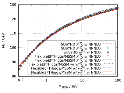
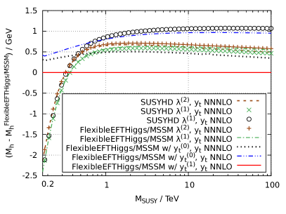
Figure 1: Influence of switching on or off different contributions to the lightest CP-even Higgs pole mass, $M_{h}$, in SusyHD and FlexibleEFTHiggs for $\tan\beta=5$, $X_{t}=0$.

Figure 1 compares FlexibleEFTHiggs to SusyHD. It demonstrates the validity of FlexibleEFTHiggs and shows the numerical impact of the various different design choices made in FlexibleEFTHiggs and SusyHD. The red solid line shows $M_{h}$ as a function of $M_{\text{SUSY}}$ for FlexibleEFTHiggs with maximum precision, i.e. with 1-loop mass matching conditions Eqs. (20)–(25) at the scale $M_{\text{SUSY}}$, 3-loop running in the Standard Model, 1-loop matching to the known low-energy parameters, including 2-loop QCD corrections to $y_{t}^{\text{SM}}$. The other lines correspond to SusyHD and variants of FlexibleEFTHiggs, where the SusyHD-like calculation is transformed step by step into the FlexibleEFTHiggs-like one. We will now explain each step in detail.

• The brown dashed line corresponds to SusyHD with maximum precision. The brown pluses correspond to FlexibleEFTHiggs, where the calculation of all Standard Model parameters is performed using the same expressions as in SusyHD. This means in particular that the fit formulas of Ref. [69] are used to obtain the running gauge and Yukawa couplings at the $M_{t}$ scale. Thus, both programs use 2-loop threshold corrections to $\lambda(M_{\text{SUSY}})$ from Eq. (18), 3-loop running in the Standard Model, calculation of $\alpha_{s}^{\overline{\text{MS}},\text{SM}}(M_{t})$ using 4-loop QCD and 2-loop electroweak running from $M_{Z}$ to $M_{t}$ plus 3-loop matching, and calculation of $y_{t}^{\text{SM}}(M_{t})$ at NNNLO [69]. The two programs agree exactly with each other.

• The green crosses and the green dash-dotted line correspond to SusyHD and the modified FlexibleEFTHiggs respectively with only 1-loop matching of $\lambda$ at the high scale $M_{\text{SUSY}}$. The numerical difference from what would result from 2-loop matching is very small for large $M_{\text{SUSY}}$, namely below $50\,\text{MeV}$ for $M_{\text{SUSY}}>2\,\text{TeV}$. This confirms the statement that the 2-loop threshold correction is negligible for $X_{t}=0$ and a common SUSY mass scale.

• The black dotted line corresponds to replacing the $\lambda$-matching, Eq. (18), by the matching procedure of FlexibleEFTHiggs, Eqs. (20)–(25), except that the equality of the top pole masses at $M_{\text{SUSY}}$ has been required at the tree-level only. The Higgs pole mass matching is the essential design choice of FlexibleEFTHiggs. The line converges to the $\lambda$-matching curves for large $M_{\text{SUSY}}$, confirming that the two matching procedures become equivalent for $M_{\text{SUSY}}\to\infty$. For $M_{\text{SUSY}}\lesssim 500\,\text{GeV}$ the SusyHD-approach becomes unreliable. The difference between the two matching procedures is formally of ${\cal O}((\text{tree-level, 1-loop})\times{v^{2}}/{M_{\text{SUSY}}^{2}})$. Terms of this order are ignored in SusyHD, but correctly taken into account in FlexibleEFTHiggs, so the difference between the two matching procedures is a measure of part of the theory uncertainty of SusyHD. In Ref. [45] this theory uncertainty was labelled “EFT uncertainty”, and the numerical result of Figure 1 is compatible with the uncertainty estimate given in Ref. [45]: For the scenario shown in Figure 1 and $M_{\text{SUSY}}>1\,\text{TeV}$ the difference is smaller than $200\,\text{MeV}$. For $M_{\text{SUSY}}<500\,\text{GeV}$ the difference can reach up to $3\,\text{GeV}$.

• In the blue dashed-double-dotted line the low-scale computation of the running SM top Yukawa coupling has been changed, and the leading 3-loop QCD terms included so far have been switched off. Even though the impact on the Higgs mass is formally of 4-loop order, the resulting numerical difference is rather sizeable, around $600\,\text{MeV}$. The importance of the 3-loop corrections to the top Yukawa coupling was already stressed in Refs. [73, 69, 45]. The black circles represent the equivalent change in SusyHD, where the 3-loop QCD corrections to the SM top Yukawa coupling are switched off. In SusyHD the omission of this 3-loop correction leads to a change of the same size.

• The red line shows the calculation in FlexibleEFTHiggs. It differs from the blue dashed-double-dotted line in the following ways: (i) $y_{t}^{\text{MSSM}}(M_{\text{SUSY}})$ is calculated by matching the top pole mass at the 1-loop level (including 2-loop SM-QCD corrections) at $M_{\text{SUSY}}$ using Eq. (25), (ii) $M_{h}$ is calculated at the scale $M_{t}$ by numerically solving Eq. (17) using the full momentum-dependent 1-loop Higgs self-energy, instead of setting the momentum to the $\overline{\text{MS}}$ Higgs mass, $p^{2}=m_{h}^{2}$, as done in SusyHD. The inclusion of both changes leads to an approximately constant decrease of $M_{h}$ of about $1\,\text{GeV}$.

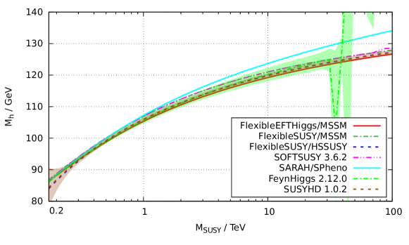
Figure 2: Comparison of predictions for $M_{h}$ in the MSSM using the EFT with pole mass matching method (FlexibleEFTHiggs/MSSM), the pure EFT calculation (FlexibleSUSY/HSSUSY and SusyHD) and the diagrammatic calculations (FlexibleSUSY/MSSM, SARAH/SPheno, SOFTSUSY and FeynHiggs) for $\tan\beta=5$ and $X_{t}=0$. The green and brown bands show the theory uncertainty as estimated by FeynHiggs and SusyHD, respectively.

Figure 2 compares the results of FlexibleEFTHiggs and SusyHD/HSSUSY to the fixed-order results of SOFTSUSY, SARAH/SPheno, and the original FlexibleSUSY. For comparison, also the results of FeynHiggs are shown; the differences between the recent versions of FeynHiggs and other calculations have been discussed e.g. in Refs. [20, 45, 3]. In line with the discussion of Figure 1, SusyHD and FlexibleEFTHiggs agree up to $0.5\,\text{GeV}$ at high $M_{\text{SUSY}}$, but SusyHD deviates more strongly at low $M_{\text{SUSY}}$ due to the missing terms of ${\cal O}((\text{tree-level, 1-loop})\times{v^{2}}/{M_{\text{SUSY}}^{2}})$.

Figure 2 shows in addition that FlexibleEFTHiggs agrees at low $M_{\text{SUSY}}$ with all fixed-order calculations. This is the consequence of the choice of the pole-mass matching condition Eq. (20), and it reflects the fact that FlexibleEFTHiggs corresponds to an exact 1-loop calculation plus resummation of higher-loop logarithms.

3.1.2 Theory uncertainty estimations

The comparisons shown in the previous figures allow us to make several observations about various ways to estimate theory uncertainties. Ref. [45] has divided the theory uncertainty of SusyHD into three parts, one of which is the “EFT uncertainty” due to truncating the low-energy EFT at the dimension-4 level (i.e. taking the renormalizable SM as the EFT). This EFT uncertainty arises from missing power-suppressed terms of ${\cal O}((\text{tree-level, 1-loop})\times{v^{2}}/{M_{\text{SUSY}}^{2}})$; hence it becomes large for $M_{\text{SUSY}}\lesssim 500\,\text{GeV}$. As mentioned in the context of Figure 1, the choice of the Higgs pole mass matching condition in FlexibleEFTHiggs avoids this uncertainty by construction. As a consequence, the difference between SusyHD and FlexibleEFTHiggs at low $M_{\text{SUSY}}$ can be regarded as a measure of the EFT uncertainty of SusyHD.

In FlexibleEFTHiggs the Higgs mass prediction is exact at the 1-loop level due to the 1-loop Higgs pole mass matching condition. At the 2-loop level, power-suppressed as well as non-power-suppressed (but non-logarithmic) terms are missing; these will be discussed in the next subsection.

Now we turn to an extensive discussion of the differences between EFT and fixed-order calculations at high $M_{\text{SUSY}}$, and on the resulting theory uncertainty of the fixed-order calculations. Figure 2 shows that at high $M_{\text{SUSY}}$, the two fixed-order calculations of SPheno and FlexibleSUSY/SOFTSUSY deviate significantly from each other, and that FlexibleSUSY/SOFTSUSY agrees well with the EFT calculations. These differences originate from $\geq 3$-loop terms, which are taken into account differently. For a deeper understanding and illustration, we derive the leading 3-loop logarithms for all these approaches:

• The all-order leading-log part of the EFT results of FlexibleEFTHiggs  and SusyHD can be obtained analytically by integrating 1-loop RGEs and using tree-level matching at the high and low scales.

• SPheno, SOFTSUSY and FlexibleSUSY do a fixed-order 2-loop computation of $M_{h}$ in the $\overline{\text{DR}}$-scheme at the scale $M_{\text{SUSY}}$. Once the running parameters at the scale $M_{\text{SUSY}}$ are replaced by their low-energy counterparts via the definitions of Section 2.2, implicit terms of $\geq 3$-loop order are generated. These implicit higher-order terms are different in FlexibleSUSY/SOFTSUSY and SPheno, because of the different definitions of the top Yukawa coupling in Eqs. (13), (16), respectively.

The leading logarithms in $\alpha_{s}$ and $\alpha_{t}$ up to 3-loop level obtained in these ways can be written as

$$\begin{split}(M_{h}^{2})^{X}&=m_{h}^{2}+\hat{v}^{2}\hat{y}_{t}^{4}\Big{[}12t_{S}\kappa_{L}-12t_{S}^{2}\kappa_{L}^{2}\left(16\hat{g}_{3}^{2}-3\hat{y}_{t}^{2}\right)+4t_{S}^{3}\kappa_{L}^{3}\Delta^{X}_{\text{3LLL}}+\cdots\Big{]},\\ \Delta^{X}_{\text{3LLL}}&=\begin{cases}736\hat{g}_{3}^{4}-240\hat{g}_{3}^{2}\hat{y}_{t}^{2}-99\hat{y}_{t}^{4}&(X=\text{EFT}),\\ \frac{736}{3}\hat{g}_{3}^{4}+144\hat{g}_{3}^{2}\hat{y}_{t}^{2}-\frac{351}{2}\hat{y}_{t}^{4}&(X=\text{$\text{FlexibleSUSY}$/$\text{SOFTSUSY}$}),\\ \frac{992}{3}\hat{g}_{3}^{4}+240\hat{g}_{3}^{2}\hat{y}_{t}^{2}-\frac{297}{2}\hat{y}_{t}^{4}&(X=\text{$\text{SPheno}$}),\end{cases}\end{split}$$ (28)

where $X$ denotes the calculational approach ($X=\text{EFT}$ denotes FlexibleEFTHiggs or SusyHD) and $\kappa_{L}=1/(16\pi^{2})$, $t_{S}=\ln(M_{\text{SUSY}}/M_{t})$, $\hat{v}=v^{\text{SM}}(M_{t})$, $\hat{g}_{3}=g_{3}^{\text{SM}}(M_{t})$, $\hat{y}_{t}=y_{t}^{\text{SM}}(M_{t})$. We have worked in the large-$\tan\beta$ limit, and the details of this calculation are shown in Appendix B; for the EFT-case similar analytical results including subleading logarithms are presented in Refs. [42, 43].

By construction, all codes agree at the 2-loop level, and the EFT calculations contain the correct 3-loop leading log. However, the implicit 3-loop leading logs of SPheno and FlexibleSUSY/SOFTSUSY in (28) are both incorrect, and different.

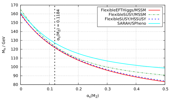
Figure 3: Accidentality of the agreement between EFT and ($\overline{\text{DR}}$) fixed-order results: $M_{h}$ in the MSSM as a function of $\alpha_{s}^{\overline{\text{MS}},\text{SM(5)}}(M_{Z})$ for $M_{\text{SUSY}}=20\,\text{TeV}$, $\tan\beta=5$, $X_{t}=0$, $M_{t}=173.34\,\text{GeV}$, $m_{b}^{\overline{\text{MS}},\text{SM(5)}}(m_{b})=\frac{4.18\,\text{GeV}}{100}$, $M_{\tau}=\frac{1.777\,\text{GeV}}{100}$.

The analytical results show why FlexibleSUSY/SOFTSUSY and SPheno deviate from each other at high $M_{\text{SUSY}}$. They also make it clear that the difference between FlexibleSUSY/SOFTSUSY and SPheno should be regarded as part of the theory uncertainty of both programs. In fact, inspection of the coefficients of the 3-loop leading logs in Eqs. (28) indicates that the theory uncertainty of both FlexibleSUSY/SOFTSUSY and SPheno could be significantly larger than their difference. In this sense it is surprising that the EFT results are actually close to FlexibleSUSY/SOFTSUSY but far away from SPheno in Figure 2. The reason for this is an accidental cancellation between the ${\cal O}(\alpha_{s}^{2}\alpha_{t})$ terms in Eqs. (28) and formally subleading terms. This cancellation can be made more obvious, if one expresses $M_{h}$ in terms of the Standard Model $\overline{\text{MS}}$ parameters at $M_{\text{SUSY}}$:

$$(M_{h}^{2})^{X} =m_{h}^{2}+v^{2}y_{t}^{4}\Big{[}12t_{S}\kappa_{L}+12t_{S}^{2}\kappa_{L}^{2}\left(16{g}_{3}^{2}-9y_{t}^{2}\right)+4t_{S}^{3}\kappa_{L}^{3}\bar{\Delta}^{X}_{\text{3LLL}}+\ldots\Big{]},$$

$$\bar{\Delta}^{X}_{\text{3LLL}} =\begin{cases}736{g}_{3}^{4}-672{g}_{3}^{2}y_{t}^{2}+90y_{t}^{4}&(X=\text{EFT}),\\ \frac{736{g}_{3}^{4}}{3}-288{g}_{3}^{2}y_{t}^{2}+\frac{27y_{t}^{4}}{2}&(X=\text{$\text{FlexibleSUSY}$/$\text{SOFTSUSY}$}),\\ \frac{992{g}_{3}^{4}}{3}-192{g}_{3}^{2}y_{t}^{2}+\frac{81y_{t}^{4}}{2}&(X=\text{$\text{SPheno}$}),\end{cases}$$ (29)

where $v=v^{\text{SM}}(M_{\text{SUSY}})$, ${g}_{3}=g_{3}^{\text{SM}}(M_{\text{SUSY}})$, $y_{t}=y_{t}^{\text{SM}}(M_{\text{SUSY}})$. In the EFT result there is an accidental, numerical cancellation between the different 3-loop terms which has been observed and discussed in Refs. [42, 43]. In spite of different numerical coefficients, a similar cancellation happens in FlexibleSUSY/SOFTSUSY and (to a smaller extent) in SPheno. As a consequence, the EFT results are closer to the fixed-order ones than what could be expected.

To highlight this accidentality we show Figure 3, which displays $M_{h}$ in the three approaches for different values of $\alpha_{s}^{\overline{\text{MS}},\text{SM(5)}}(M_{Z})$. $M_{\text{SUSY}}$ is set to $20\,\text{TeV}$ to amplify the 3-loop leading logarithms. The plot shows that accidentally the fixed-order FlexibleSUSY and the EFT calculations agree around the true value of $\alpha_{s}^{\overline{\text{MS}},\text{SM(5)}}(M_{Z})\approx 0.1184$.

Figure 4: Illustration of the theory uncertainty estimate $\Delta M_{h}^{(4\times y_{t})}$ of the fixed-order calculations of FlexibleSUSY and SARAH/SPheno using four different ways to calculate $y_{t}^{\text{MSSM}}$. We choose $\tan\beta=5$ and $X_{t}=0$. The red band shows the variation of $M_{h}$ when the coefficient $C_{1}$ is varied within the interval $[-184/9,184/9]$. The yellow uncertainty band shows $\Delta M_{h}^{(Q)}$, defined as the variation of $M_{h}$ when the renormalization scale at which $M_{h}$ is calculated is varied within $[M_{\text{SUSY}}/2,2M_{\text{SUSY}}]$.

After these considerations we turn to the question of estimating the theory uncertainty of the $\overline{\text{DR}}$ fixed-order calculations. As noted above, the difference between the fixed-order MSSM calculations in FlexibleSUSY/SOFTSUSY and SPheno is due to a different treatment of the 3-loop leading logarithms, so it can be regarded as an estimate for part of the theory uncertainty of the two calculations. On a more general level, we therefore discuss two ways to estimate the theory uncertainty of these fixed-order calculations:

1. Using known MSSM higher-order results:

In the MSSM, we know that the leading 1-loop contributions are governed by the running top mass $m_{t}$. On the other hand the full 2-loop MSSM SUSY-QCD contributions to $m_{t}$ are known [68]. Evaluating Eq. (13) at the 2-loop leading log level taking into account the full 2-loop SUSY-QCD contributions of [68] would shift the running top mass by

$$\Delta m_{t}^{(2)}(M_{Z})=-\frac{184}{9}\frac{g_{3}^{4}M_{t}}{(4\pi)^{4}}\ln^{2}\frac{M_{\text{SUSY}}}{M_{Z}}.$$ (30)

Thus, to estimate the theory uncertainty, we can add the term

$$C_{1}\frac{g_{3}^{4}M_{t}}{(4\pi)^{4}}\ln^{2}\frac{M_{\text{SUSY}}}{M_{Z}}$$ (31)

to the r.h.s. of Eq. (13) and vary the coefficient $C_{1}$ within the interval $[-184/9,184/9]$. This changes the 3-loop leading logarithms in the Higgs boson mass prediction by a motivated amount. The resulting uncertainty band is shown in red in Figure 4. We find that this uncertainty band contains both the FlexibleSUSY curve (green dash-dotted line) and the SPheno curve (turquoise solid line).

2. Generating higher-order terms:

Another option is to change the calculation of $y_{t}^{\text{MSSM}}$ such that changes of higher-order are automatically induced. The different treatment of $y_{t}^{\text{MSSM}}$ in FlexibleSUSY and SPheno, i.e. using Eq. (13) or (16), provides two examples. There are further motivated possibilities to define $y_{t}^{\text{MSSM}}$, namely to employ either Eq. (13) or Eq. (16) at the renormalization scale $M_{\text{SUSY}}$ instead of at $M_{Z}$. All four variants to calculate $y_{t}^{\text{MSSM}}$ are equal at the 1-loop level but different at the 2-loop level, so the resulting Higgs masses differ by 3-loop terms. In Figure 4 we show the four corresponding Higgs mass predictions. The two new ones are shown as the black dashed line and the brown dotted line, respectively. We find that the four approaches to calculate $y_{t}^{\text{MSSM}}$ are distributed within the red uncertainty band. Their differences thus represent an alternative way to estimate the theory uncertainty from the missing 3-loop leading logarithms in the fixed-order calculations. We therefore define

$$\Delta M_{h}^{(4\times y_{t})}=\max_{y_{t}^{(i)},\,y_{t}^{(j)}\in\left\{y_{t}^{\eqref{eq:fixedmt_FlexibleSUSY}}(M_{Z}),y_{t}^{\eqref{eq:fixedmt_SPheno}}(M_{Z}),y_{t}^{\eqref{eq:fixedmt_FlexibleSUSY}}(M_{\text{SUSY}}),y_{t}^{\eqref{eq:fixedmt_SPheno}}(M_{\text{SUSY}})\right\}}\left|M_{h}(y_{t}^{(i)})-M_{h}(y_{t}^{(j)})\right|,$$ (32)

where $y_{t}^{\eqref{eq:fixedmt_FlexibleSUSY}}(Q)$ refers to the definition of Eq. (13) and $y_{t}^{\eqref{eq:fixedmt_SPheno}}(Q)$ refers to Eq. (16) evaluated at the scale $Q$. The advantage of this second way is that it can be applied also in non-minimal models, where the 2-loop contributions to $y_{t}^{\text{SUSY}}$ are unknown.

Another frequently used way to estimate the theory uncertainty is to vary the renormalization scale $Q$ at which $M_{h}$ is calculated and the loop-corrected EWSB conditions are solved. The variation interval is usually chosen to be $[Q_{0}/2,2Q_{0}]$, where $Q_{0}$ is the default renormalization scale to be used to calculate the Higgs pole mass in the chosen approach. In the fixed-order programs $Q_{0}=M_{\text{SUSY}}$ is used, while in FlexibleEFTHiggs we use $Q_{0}=M_{t}$.

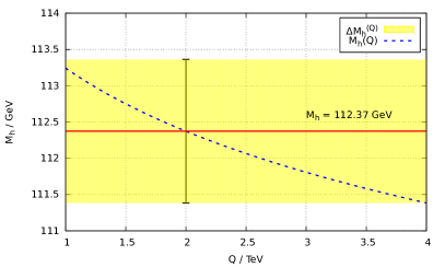
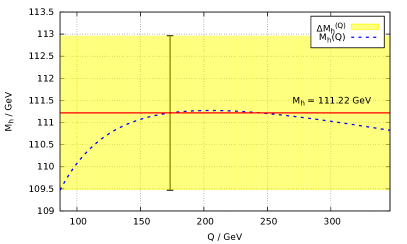
Figure 5: Illustration of the theory uncertainty estimate $\Delta M_{h}^{(Q)}$ for the fixed-order calculations of FlexibleSUSY and SARAH/SPheno (left panel) as well as FlexibleEFTHiggs (right panel). The blue dashed line shows $M_{h}$ in the MSSM for $\tan\beta=5$, $X_{t}=0$, $M_{\text{SUSY}}=2\,\text{TeV}$ as a function of the renormalization scale $Q$. The black vertical error bar is placed at the default value of the renormalization scale, $Q_{0}$, and the red horizontal line marks the corresponding Higgs pole mass, $M_{h}(Q_{0})$. The black error bar and the yellow band show the resulting uncertainty estimate $\Delta M_{h}^{(Q)}$.

Figure 5 shows $M_{h}$ as a function of $Q$ in the MSSM calculated for $\tan\beta=5$, $X_{t}=0$, $M_{\text{SUSY}}=2\,\text{TeV}$ with FlexibleSUSY in the fixed-order approach (left panel) and with FlexibleEFTHiggs (right panel). The renormalization scale has been varied within the interval $[Q_{0}/2,2Q_{0}]$. In each approach one can see that the sizes of the resulting upwards and downwards variations of the Higgs pole mass is not equal and might even be highly non-linear. Due to this effect, we define the uncertainty $\Delta M_{h}^{(Q)}$ to be

$$\Delta M_{h}^{(Q)}=\max_{Q\in[Q_{0}/2,2Q_{0}]}\left|M_{h}(Q_{0})-M_{h}(Q)\right|.$$ (33)

Thus, in this scenario we obtain $\Delta M_{h}^{(Q)}=1.0\,\text{GeV}$ for the fixed-order approach, and $\Delta M_{h}^{(Q)}=1.7\,\text{GeV}$ for FlexibleEFTHiggs. The yellow band in Figure 4 shows the variation of $M_{h}$ in the fixed-order approach when $Q$ is varied within the interval $[M_{\text{SUSY}}/2,2M_{\text{SUSY}}]$.

By construction, the width of this band, i.e. the magnitude of $2\times\Delta M_{h}^{(Q)}$ is given by terms of ${\cal O}(\text{3-loop}\times\ln^{2}(M_{\text{SUSY}}/M_{Z})\times\ln(2))$ or ${\cal O}(\text{2-loop}\times\ln(M_{\text{SUSY}}/M_{Z})\times\ln(2))$, where in the latter case only 2-loop contributions beyond the ${\mathcal{O}}((\alpha_{t}+\alpha_{b})^{2}+(\alpha_{t}+\alpha_{b})\alpha_{s}+\alpha_{\tau}^{2})$ can contribute. This should be contrasted with the magnitude of $\Delta M_{h}^{(4\times y_{t})}$ from (32), which is a measure of the leading missing/incorrect terms of ${\cal O}(\text{3-loop}\times\ln^{3}(M_{\text{SUSY}}/M_{Z}))$. Hence the two uncertainty estimations are sensitive to different contributions, but particularly $\Delta M_{h}^{(Q)}$ alone would underestimate the theory uncertainty at high $M_{\text{SUSY}}$.

3.2 MSSM for $\boldsymbol{X_{t}\neq 0}$

3.2.1 Results of FlexibleEFTHiggs and fixed-order calculations

Now we turn to the MSSM with $X_{t}\neq 0$. The main new aspect is that the 2-loop threshold correction for $\lambda(M_{\text{SUSY}})$, which is not implemented in FlexibleEFTHiggs, is now non-negligible. Hence, we can in particular discuss the theory uncertainty of FlexibleEFTHiggs from these missing non-logarithmic 2-loop contributions. However, our analysis is intended to be more general. It aims to be applicable also to the case of the non-minimal SUSY models discussed in the subsequent sections, as well as in the future when the 2-loop threshold correction is implemented in FlexibleEFTHiggs. It might also shed light on the theory uncertainty of existing programs such as SusyHD.

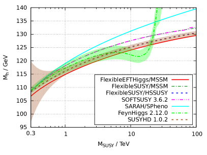
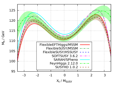
Figure 6: Comparison of predictions for $M_{h}$ in the MSSM using the EFT with pole mass matching method (FlexibleEFTHiggs/MSSM), the pure EFT calculation (FlexibleSUSY/HSSUSY and SusyHD) and the diagrammatic calculations (FlexibleSUSY/MSSM, SARAH/SPheno, SOFTSUSY and FeynHiggs) for $\tan\beta=5$. The green and brown bands show the theory uncertainty as estimated by FeynHiggs and SusyHD, respectively. In the left panel we fix $X_{t}=-2M_{\text{SUSY}}$ and vary $M_{\text{SUSY}}$. In the right panel we fix $M_{\text{SUSY}}=2\,\text{TeV}$ and vary $X_{t}$.

In Figure 6 we show $M_{h}$ in the MSSM as a function of $M_{\text{SUSY}}$ for $X_{t}=-2M_{\text{SUSY}}$ in the left panel, and $M_{h}$ as a function of $X_{t}$ for $M_{\text{SUSY}}=2\,\text{TeV}$ in the right panel, for some publicly available spectrum generators. The Higgs boson mass is calculated using FlexibleEFTHiggs (red solid line), FlexibleSUSY (green dash-dotted line), SOFTSUSY (pink dashed-double-dotted line), SARAH/SPheno (turquoise solid line), FeynHiggs (light green dash-dotted line) and SusyHD (brown dashed line).

The large difference between SPheno and FlexibleSUSY/SOFTSUSY in these two figures is again due to the different, incorrect $\geq 3$-loop leading logs. As Figure 6 shows, the difference is increasing with $M_{\text{SUSY}}$, and thus should be regarded as an estimate of part of the theory uncertainty of SPheno and FlexibleSUSY/SOFTSUSY.

For $X_{t}=0$, SusyHD and FlexibleEFTHiggs differ by around $1\,\text{GeV}$, which corresponds mainly to the inclusion of higher-order terms in the matching of $y_{t}$ at $M_{\text{SUSY}}$, to 1-loop terms suppressed by ${v^{2}}/{M_{\text{SUSY}}^{2}}$, which are missing in SusyHD, and to the different definition of the running top mass at the low scale. As can be seen in Figure 6, for $X_{t}\neq 0$ the difference between SusyHD and FlexibleEFTHiggs can become larger, due to the missing 2-loop $M_{h}$ matching in FlexibleEFTHiggs. Still, in accordance with the non-logarithmic nature of the 1-loop threshold corrections, the difference between SusyHD and FlexibleEFTHiggs does not significantly increase with $M_{\text{SUSY}}$.

3.2.2 Theory uncertainty estimations

Now we turn to estimating the theory uncertainty of FlexibleEFTHiggs. As explained in Section 3.1.2 it has no “EFT uncertainty”, because power-suppressed terms are automatically taken into account up to the 1-loop level. But FlexibleEFTHiggs is missing the 2-loop threshold corrections in its current version, leading to a theory uncertainty. We propose several methods to estimate the theory uncertainty of $M_{h}$ in FlexibleEFTHiggs originating from these missing 2-loop threshold corrections:

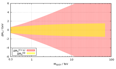
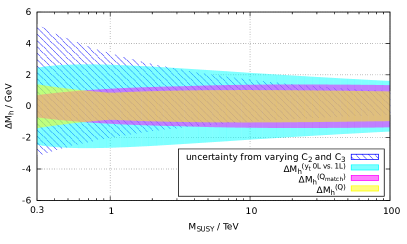
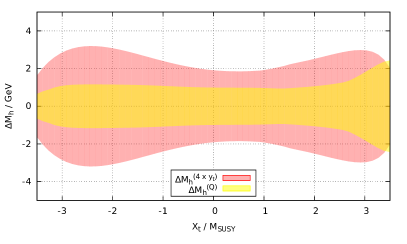
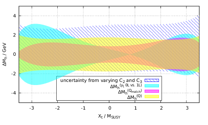
Figure 7: Uncertainty estimates for the fixed-order 2-loop calculations with FlexibleSUSY and SARAH/SPheno and for FlexibleEFTHiggs. Left panels: fixed-order uncertainty estimates of Sec. 3.1.2 using renormalization scale variation, $\Delta M_{h}^{(Q)}$ (yellow) and from the different top Yukawa definitions, $\Delta M_{h}^{(4\times y_{t})}$ (red). Right panels: FlexibleEFTHiggs uncertainty estimations of Sec. 3.2.2 using renormalization scale uncertainty, $\Delta M_{h}^{(Q)}$ (yellow), matching scale variation, $\Delta M_{h}^{(Q_{\text{match}})}$ (pink) and the uncertainty from different loop orders for the top pole mass matching, $\Delta M_{h}^{(y_{t}\text{ 0L vs.\ 1L})}$ (turquoise). In the top row $\tan\beta=5$ and $X_{t}=-2M_{\text{SUSY}}$ is used. In the bottom row we set $\tan\beta=5$ and $M_{\text{SUSY}}=2\,\text{TeV}$.

1. Using known MSSM higher-order results:

Actually the leading MSSM 2-loop threshold corrections for $\lambda(M_{\text{SUSY}})$ are known and are of ${\cal O}(\alpha_{t}\alpha_{s})$ and $\mathcal{O}(\alpha_{t}^{2})$ [44, 45]. They have the form

$$\Delta\lambda^{(2)}_{(\alpha_{t}\alpha_{s})} =\frac{g_{3}^{2}(y_{t}^{\text{SM}})^{4}}{(4\pi)^{4}}\times C_{2}, \Delta\lambda^{(2)}_{(\alpha_{t}^{2})} =\frac{(y_{t}^{\text{SM}})^{6}}{(4\pi)^{4}}\times C_{3},$$ (34)

where the coefficients $C_{2}$ and $C_{3}$ depend on $Q_{\text{match}}$, $X_{t}/M_{\text{SUSY}}$ and $\tan\beta$ in our common SUSY mass scale scenario. If one sets $Q_{\text{match}}=M_{\text{SUSY}}$ and varies $X_{t}$ within the reasonably large interval $[-3M_{\text{SUSY}},+3M_{\text{SUSY}}]$ and $\tan\beta$ within $[1,\infty]$, the coefficients vary within $C_{2}\in[-314,231]$ and $C_{3}\in[-6,489]$. These minimal and maximal values for $C_{2}$ and $C_{3}$ can be used to estimate the maximal effect of the missing 2-loop threshold corrections to $\lambda(M_{\text{SUSY}})$ in FlexibleEFTHiggs by adding the terms (34) to the r.h.s. of Eq. (22). The uncertainty estimated in this way is shown as the dashed area in the panels on the r.h.s. of Figure 7. As can also be seen from Figure 6, the variation of $C_{2}$ and $C_{3}$ does not reflect the fact that the 2-loop threshold corrections are negligible for $X_{t}=0$ and are large for $X_{t}\approx\sqrt{6}M_{\text{SUSY}}$. Therefore, the variation of $C_{2}$ and $C_{3}$ certainly leads to an overestimation of the theory uncertainty of FlexibleEFTHiggs for small values of $X_{t}$. However, one can expect that the theory uncertainty estimated in this way is reasonable for maximal mixing scenarios.

2. Generating higher-order terms:

Another option to estimate the uncertainty is to change the calculation of $\lambda(M_{\text{SUSY}})$ in FlexibleEFTHiggs such that changes of higher-order are automatically induced. Here we have two quantities at our disposal, which we expect to have a sizable impact on the value of $\lambda(M_{\text{SUSY}})$: (i) the value of $y_{t}^{\text{MSSM}}$, (ii) the choice of the renormalization scale, $Q_{\text{match}}$, at which $\lambda$ is calculated.

• The dominant 1-loop threshold correction to $\lambda$ is governed by the top Yukawa coupling. Thus, changing $y_{t}$ by motivated 1-loop terms shifts $\lambda$ by 2-loop terms. Such motivated terms can be obtained by switching the $y_{t}^{\text{MSSM}}$ definition at the SUSY scale, Eq. (25), between the 1-loop level and the tree-level. The differences in $y_{t}^{\text{MSSM}}$ are sensitive to $\alpha_{s}$, $\alpha_{t}$, $X_{t}$, and contain logarithmic as well as non-logarithmic terms. The resulting shift in $\lambda$ should therefore provide a good estimate of the magnitude of the actual dominant 2-loop threshold corrections to $\lambda$. As an automatic way to evaluate the theory uncertainty from the missing 2-loop threshold corrections we propose to define

  $$\Delta M_{h}^{(y_{t}\text{ 0L vs.\ 1L})}=\left|M_{h}^{\text{$\text{FlexibleEFTHiggs}$}}(y_{t}^{\text{MSSM},(1)})-M_{h}^{\text{$\text{FlexibleEFTHiggs}$}}(y_{t}^{\text{MSSM},(0)})\right|,$$ (35)

  where the two terms on the r.h.s. correspond to the FlexibleEFTHiggs prediction using the $y_{t}^{\text{MSSM}}(M_{\text{SUSY}})$ definition (25) either at the 1-loop or at the tree-level.

  The turquoise uncertainty band in the panels on the r.h.s. of Figure 7 shows the variation of $M_{h}$ by $\pm\Delta M_{h}^{(y_{t}\text{ 0L vs.\ 1L})}$, i.e. the variation from using either the tree-level or 1-loop top Yukawa coupling. The figures show that this estimated uncertainty is of the same order as the uncertainty obtained from variation of $C_{2}$ and $C_{3}$ for most SUSY scales. Furthermore, we find that the uncertainty estimate vanishes for $X_{t}\approx 0$ and is maximal for maximal mixing ($X_{t}\approx\pm\sqrt{6}M_{\text{SUSY}}$). Thus, this estimated uncertainty reflects the expectation that the missing 2-loop threshold corrections for $\lambda(M_{\text{SUSY}})$ are small for vanishing $X_{t}$ and can be sizable for maximal mixing.

• By variation of the matching scale $Q_{\text{match}}$ within the interval $[M_{\text{SUSY}}/2,2M_{\text{SUSY}}]$, the size of logarithmic higher-order contributions to $\lambda(M_{\text{SUSY}})$ can be estimated. Varying $Q_{\text{match}}$ involves (a) RG running of all Standard Model parameters to $Q_{\text{match}}$ using 3-loop RGEs, (b) RG running of all MSSM parameters to $Q_{\text{match}}$ using 2-loop RGEs and (c) calculation of $\lambda$, as well as the MSSM gauge and Yukawa couplings and $v^{\text{MSSM}}$ at the scale $Q_{\text{match}}$ using Eqs. (20)–(25). Thus, the matching scale variation is sensitive to missing 2-loop renormalization scale-dependent logarithmic contributions in the calculation of $\lambda$.

  The effect of the matching scale variation is shown by the red band on the r.h.s. of Figure 7. We find that the uncertainty is nearly independent of $X_{t}$, which is in agreement with the expectation: As can be seen from Eq. (71), the renormalization scale-dependent part of the 1-loop threshold correction, $\Delta\lambda^{(1)}$, is not $X_{t}$-dependent. Furthermore, the $\beta$ functions of the MSSM parameters $g_{Y}^{\text{MSSM}}$, $g_{2}^{\text{MSSM}}$, $\tan\beta$, $v_{u}$ and $v_{d}$, which determine $\lambda$ at the tree-level, do not depend on $X_{t}$ either [74, 75]. For this reason, the variation of $Q_{\text{match}}$ is not directly sensitive to $X_{t}$-dependent terms. Therefore, one can expect that the variation of $Q_{\text{match}}$ alone is not sufficient to estimate the theory uncertainty from missing 2-loop threshold corrections.

Another source of uncertainty in FlexibleEFTHiggs comes from the missing 2-loop contributions to $M_{h}$ in the SM. As done above, one way to estimate the leading logarithmic 2-loop $M_{h}$ contributions is to vary the renormalization scale $Q$, at which $M_{h}$ is calculated, within the interval $[M_{t}/2,2M_{t}]$. This uncertainty estimate is shown in form of the yellow band on the r.h.s. of Figure 7. Comparing all uncertainty bands for FlexibleEFTHiggs, we find that for this scenario the Higgs mass theory uncertainty is dominated by the missing 2-loop contributions to $\lambda(M_{\text{SUSY}})$.

4 Combined MSSM uncertainty estimation

In the previous section we discussed many different ways to estimate contributions to theory uncertainties, relevant for existing fixed-order calculations as well as for SusyHD and FlexibleEFTHiggs. In this section we summarize and combine these various uncertainty estimates, focusing on FlexibleEFTHiggs and the fixed-order codes (the discussion equally applies to FlexibleSUSY, SOFTSUSY and SPheno). Figure 8 shows the Higgs pole mass calculated with FlexibleEFTHiggs and the fixed-order FlexibleSUSY, including estimates of theory uncertainties. The plots demonstrate that the new approach always has an uncertainty of around 2–3 GeV and becomes more accurate for $M_{\text{SUSY}}$ in the few-TeV range. We now provide the details of the uncertainty estimates.

FlexibleEFTHiggs calculation:

Following the classification of the theory uncertainties in Ref. [45], FlexibleEFTHiggs has two basic sources of theory uncertainty: from missing higher-order corrections in the matching procedure at the high scale (“high-scale uncertainty”), and from missing higher-order corrections in the Higgs pole mass computation in the EFT at the low scale (“low-scale uncertainty”).

An important property of FlexibleEFTHiggs is the inclusion of all non-logarithmic 1-loop contributions to $M_{h}$ due to the special choice of the matching procedure. As discussed in Section 3, the resulting “EFT uncertainty” discussed in Ref. [45] due to missing power-suppressed tree-level or 1-loop terms is therefore not present in FlexibleEFTHiggs by construction.

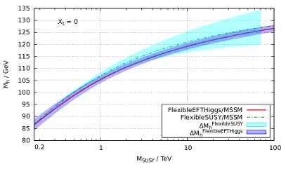
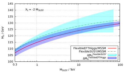
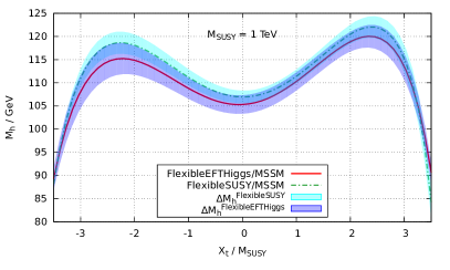
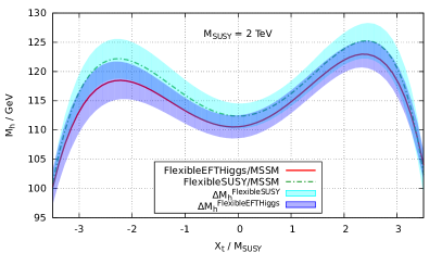
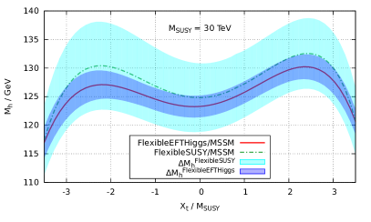
Figure 8: Predictions for $M_{h}$ and combined theoretical uncertainty estimates for FlexibleSUSY and FlexibleEFTHiggs in the MSSM for $\tan\beta=5$. The first three panels show $M_{h}$ as a function of $M_{\text{SUSY}}$ for $X_{t}/M_{\text{SUSY}}=0$, $-2$ and $2$, respectively. The last three panels show $M_{h}$ as a function $X_{t}$ for $M_{\text{SUSY}}=1\,\text{TeV}$, $2\,\text{TeV}$ and $30\,\text{TeV}$, respectively.

The high-scale uncertainty of FlexibleEFTHiggs is estimated in two ways, introduced and discussed in detail in Section 3.1.2:

1. Use of $y_{t}^{\text{MSSM}}(M_{\text{SUSY}})$, which has been obtained from the top pole mass matching at the SUSY scale either at the tree-level or at the 1-loop level. We denote the corresponding shift in the Higgs pole mass as $\Delta M_{h}^{(y_{t}\text{ 0L vs.\ 1L})}$, as defined in Eq. (35).

2. Variation of the matching scale $Q_{\text{match}}$ within the interval $[M_{\text{SUSY}}/2,2M_{\text{SUSY}}]$. We denote the corresponding Higgs pole mass uncertainty estimate by $\Delta M_{h}^{(Q_{\text{match}})}$, see Eq. (33).

The low-scale uncertainty is estimated as follows:

1. Variation of the renormalization scale $Q$, at which the Higgs pole mass is calculated, in the interval $[M_{t}/2,2M_{t}]$. We denote the corresponding Higgs pole mass uncertainty estimate by $\Delta M_{h}^{(Q)}$, see Eq. (33).

Since the two high-scale uncertainty estimates 1 and 2 are partially sensitive to the same higher-order MSSM corrections, we combine $\Delta M_{h}^{(y_{t}\text{ 0L vs.\ 1L})}$ and $\Delta M_{h}^{(Q_{\text{match}})}$ by taking the maximum of the two for each parameter point. $\Delta M_{h}^{(Q)}$ is sensitive to logarithmic higher-order Standard Model corrections, which is why we add it in quadrature to the former:

$$\Delta M_{h}^{\text{FlexibleEFTHiggs}}=\sqrt{\left(\max\left\{\Delta M_{h}^{(y_{t}\text{ 0L vs.\ 1L})},\Delta M_{h}^{(Q_{\text{match}})}\right\}\right)^{2}+\left(\Delta M_{h}^{(Q)}\right)^{2}}.$$ (36)

In Figure 8 we find that for small values of $X_{t}$ this combined uncertainty estimate is of the order $2\,\text{GeV}$ for FlexibleEFTHiggs. The uncertainty grows up to around $3\,\text{GeV}$ for maximal mixing. Since FlexibleEFTHiggs is an EFT calculation, its uncertainty does not depend on the SUSY scale: Even for large $M_{\text{SUSY}}\approx 30\,\text{TeV}$ the uncertainty is of the order or below $3\,\text{GeV}$. Likewise, because there is no “EFT uncertainty”, the uncertainty does not grow significantly for low $M_{\text{SUSY}}$.

Fixed-order calculation:

The theory uncertainty of the fixed-order calculations arises from missing higher-order corrections. As described in Section 3.1.2 we propose two measures of leading missing contributions:

1. Using the four different definitions of $y_{t}^{\text{MSSM}}$, as described in Section 3.1.2. We denote the maximum difference between the Higgs masses obtained using these four definitions as $\Delta M_{h}^{(4\times y_{t})}$, see Eq. (32). This is particularly sensitive to the leading 3-loop logarithms governed by the top Yukawa coupling.

2. Variation of the renormalization scale $Q$, at which the Higgs pole mass is calculated, within the interval $[M_{\text{SUSY}}/2,2M_{\text{SUSY}}]$. We denote the corresponding Higgs pole mass uncertainty estimate by $\Delta M_{h}^{(Q)}$, see Eq. (33). This is particularly sensitive to subleading logarithms governed by all couplings of the MSSM.

We have combined these two uncertainty estimates as

$$\Delta M_{h}^{\text{FlexibleSUSY}}=\sqrt{\left(\Delta M_{h}^{(4\times y_{t})}\right)^{2}+\left(\Delta M_{h}^{(Q)}\right)^{2}}.$$ (37)

In Figure 8, $\Delta M_{h}^{\text{FlexibleSUSY}}$ grows logarithmically with $M_{\text{SUSY}}$ as expected. For small values of $X_{t}$ and SUSY scales below $1\,\text{TeV}$, the combined uncertainty estimate is below $1\,\text{GeV}$. For larger SUSY scales and larger $X_{t}$ values, the uncertainty can grow up to $9\,\text{GeV}$.

We remark that further subleading effects, such as finite, non-logarithmic corrections arising e.g. from going beyond the ${\mathcal{O}}((\alpha_{t}+\alpha_{b})^{2}+(\alpha_{t}+\alpha_{b})\alpha_{s}+\alpha_{\tau}^{2})$ approximation at the 2-loop level, are not necessarily captured by the estimate (37); hence particularly at low $M_{\text{SUSY}}$, the true uncertainty of the fixed-order calculations might be larger than this estimate.

5 Numerical results in the NMSSM

Here we consider the next-to-minimal supersymmetric standard model (NMSSM) [76, 77], where the MSSM superfield content is extended by an extra gauge singlet superfield $\hat{S}$. In early calculations of higher-order corrections to NMSSM Higgs masses both effective field theory techniques [78, 79, 80, 81, 82, 83] and fixed-order calculations in the effective potential approximation [84, 85, 86, 87] were employed. More recently $\overline{\text{DR}}$ calculations with full 1-loop corrections  [27, 88], 2-loop corrections of ${\cal O}(\alpha_{s}(\alpha_{b}+\alpha_{t}))$ [27], and finally 2-loop corrections involving all superpotential parameters were calculated [89]. Recent progress in a mixed on-shell-$\overline{\text{DR}}$ scheme has also been made, with full 1-loop corrections [63, 64] and 2-loop corrections of ${\cal O}(\alpha_{s}\alpha_{t})$ [90].

We assume that there is a $Z_{3}$ symmetry, which forbids the $\mu$-term so that when the new scalar singlet, $S$, develops a VEV and generates an effective $\mu$-term, it solves the $\mu$ problem of the MSSM. The superpotential is then,

$$\mathcal{W}_{\textrm{NMSSM}}=\mathcal{W}_{\textrm{MSSM}}(\mu=0)+\lambda\,\hat{S}\,\hat{H}_{u}\cdot\hat{H}_{d}+\frac{1}{3}\kappa\,\hat{S}^{3}.$$ (38)

The soft breaking Lagrangian density is,

$$\mathcal{L}_{\text{NMSSM}}^{\mathrm{soft}}=\mathcal{L}_{\text{MSSM}}^{\mathrm{soft}}(B\mu=0)+\lambda A_{\lambda}SH_{u}H_{d}+\frac{1}{3}\kappa A_{\kappa}S^{3}+m_{S}^{2}|S|^{2}.$$ (39)

The Higgs fields develop VEVs,

$$\langle H_{u}\rangle =\frac{1}{\sqrt{2}}\begin{pmatrix}0\\ v_{u}\end{pmatrix}, \langle H_{d}\rangle =\frac{1}{\sqrt{2}}\begin{pmatrix}v_{d}\\ 0\end{pmatrix}, \langle S\rangle =\frac{1}{\sqrt{2}}v_{s}.$$ (40)

Here we implement our new method for predicting the Higgs mass, and our uncertainty estimates for this and the FlexibleSUSY fixed-order calculation, to the NMSSM. We then compare our FlexibleEFTHiggs calculation to the predictions using some of the publicly available software. To keep our analysis simple we set the soft-breaking squared sfermion mass parameters and gaugino masses to $M_{\text{SUSY}}$, as defined in Eqs. (10), $\tan\beta(M_{\text{SUSY}})=5$, and require that the two additional Yukawa couplings in the NMSSM are equal,

$$\lambda(M_{\text{SUSY}})=\kappa(M_{\text{SUSY}}).$$ (41)

We also require that $v_{s}$ is fixed so that $\mu_{\text{eff}}=M_{\text{SUSY}}$, i.e.

$$v_{s}(M_{\text{SUSY}})=\frac{\sqrt{2}M_{\text{SUSY}}}{\lambda(M_{\text{SUSY}})}.$$ (42)

The new trilinears are fixed to,

$$A_{\lambda}(M_{\text{SUSY}}) =\frac{1}{\lambda}\left(\frac{\sqrt{2}\tan\beta M_{\text{SUSY}}^{2}}{v_{s}(\tan^{2}\beta+1)}-\kappa\lambda\frac{v_{s}}{\sqrt{2}}\right), A_{\kappa}(M_{\text{SUSY}}) =-\frac{\sqrt{2}M_{\text{SUSY}}^{2}}{v_{s}},$$ (43)

where all $\overline{\text{DR}}$ quantities on the right hand side are evaluated at $M_{\text{SUSY}}$. The complicated expression for $A_{\lambda}$ ensures the mass of the MSSM-like CP-odd state, which appears in the CP-odd mass matrix, is equal to $M_{\text{SUSY}}$. The soft-breaking squared Higgs mass parameters $m_{H_{u}}^{2},m_{H_{d}}^{2},m_{S}^{2}$ are fixed by the EWSB minimization conditions.

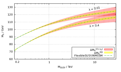
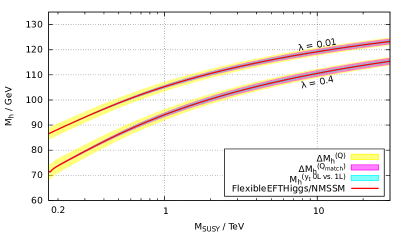
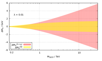
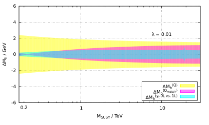
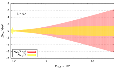
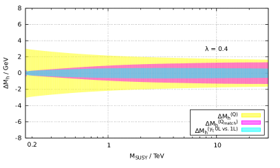
Figure 9: Higgs mass predictions and uncertainty estimates of Sec. 3 applied to the fixed-order calculations with FlexibleSUSY and to FlexibleEFTHiggs in the NMSSM. The top row shows the Higgs mass predictions and the uncertainty estimates, the lower two rows only the uncertainty estimates, as in Fig. 7. The values of the singlet Yukawa couplings are $\kappa=\lambda=0.01$ or $\kappa=\lambda=0.4$, as indicated in the plots. In all panels we have fixed $X_{t}=0$ and $\tan\beta=5$.

In Figure 9 we compare the NMSSM predictions for the Higgs mass using the FlexibleSUSY fixed-order calculation and the new FlexibleEFTHiggs calculation. In the top panels one can see that as in the MSSM the FlexibleSUSY prediction is remarkably close to FlexibleEFTHiggs. However the uncertainty bands for fixed-order calculation in the left panels of Figure 9 show that nonetheless this is a coincidence and the true uncertainty of the fixed-order calculation is much larger. Two different values of the new singlet Yukawa couplings, $\lambda$ and $\kappa$, are shown and one can see in this case increasing these couplings reduces the Higgs mass due to increased singlet mixing, but has little impact on the comparison between the two approaches.

The panels on the right of Figure 9 show the uncertainty estimation bands for the FlexibleEFTHiggs calculation. By comparing the plots in the middle panel one can see that as $M_{\text{SUSY}}$ is increased, the fixed-order uncertainty rises rapidly while the FlexibleEFTHiggs uncertainties have only a weak dependence on $M_{\text{SUSY}}$, in line with our expectations and in agreement with the results obtained in the MSSM.

If we combine these uncertainties in the manner described in Section 4, we find that also in the NMSSM FlexibleEFTHiggs becomes more precise than the fixed-order calculation for values of $M_{\text{SUSY}}$ in the few-TeV region. However, by comparing the cases $\lambda=\kappa=0.01$ and $\lambda=\kappa=0.4$ (see Figure 10) we find that the precise value of $M_{\text{SUSY}}$ at which this happens depends on the singlet Yukawa couplings.

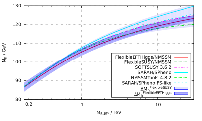
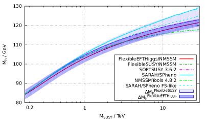
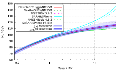
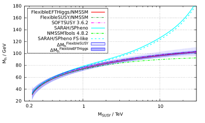
Figure 10: Predictions for $M_{h}$ and combined theoretical uncertainty estimates for FlexibleSUSY and FlexibleEFTHiggs in the NMSSM, compared with results of other codes. We choose $X_{t}=0$ and $\tan\beta=5$ in all panels. The top panel shows $\lambda=\kappa=0.01$ (left), which is close to the MSSM limit and $\lambda=\kappa=0.2$ (right). In both cases the situation is quite similar to the MSSM. Row 2 shows $\lambda=\kappa=0.4$ (left) and $\lambda=\kappa=0.6$ (right). Here we see significant deviation from the MSSM pattern with the SPheno fixed-order calculation, which is due to the same infra-red divergences behind the known Goldstone boson catastrophe [91, 92, 93].

We now turn to a comparison with the results of FlexibleEFTHiggs and various public NMSSM codes: the fixed-order FlexibleSUSY calculation, NMSPEC [28] in the NMSSMTools 4.8.2 package, the next-to-minimal extensions of SOFTSUSY 3.6.2 [25] and an NMSSM module generated with SARAH 4.9.0 and compiled and run in SPheno 3.3.8. We also include results from a modified version of SARAH/SPheno, which calculates the top quark Yukawa coupling $y_{t}^{\text{NMSSM}}(M_{Z})$ using Eq. (13) as is done in FlexibleSUSY and SOFTSUSY, labeled as SARAH/SPheno FS-like. Here we omit the calculation of NMSSMCALC [29], but one may see comparisons between NMSSMCALC calculating in the $\overline{\text{DR}}$ scheme and the other fixed-order codes in Ref. [94]. Note that the SARAH/SPheno calculations take into account the full 2-loop corrections in the gaugeless limit and effective potential approximation, while the other fixed-order codes include 2-loop NMSSM corrections of ${\mathcal{O}}((\alpha_{t}+\alpha_{b})\alpha_{s})$ from Ref. [27] but include only MSSM-like 2-loop corrections of ${\mathcal{O}}((\alpha_{t}+\alpha_{b})^{2}+\alpha_{\tau}^{2})$.

In Figure 10 we show the Higgs mass against $M_{\text{SUSY}}$ for $\lambda(M_{\text{SUSY}})=\kappa(M_{\text{SUSY}})\in\{0.01,0.2,0.4,0.6\}$. For small $\lambda$ and $\kappa$ the results are like in the MSSM. FlexibleEFTHiggs agrees very well with the fixed-order FlexibleSUSY calculation. Among the fixed-order codes, SARAH/SPheno FS-like agrees very well with SOFTSUSY and the fixed-order FlexibleSUSY. Due to the different definition of the top Yukawa coupling, the Higgs mass calculated with SPheno is slightly higher than all other fixed-order codes; NMSSMTools is slightly lower. The agreement between all these codes shows in particular that the specific, non-MSSM-like 2-loop corrections that are only included in SPheno are small.

In contrast, for larger $\lambda=\kappa\gtrsim 0.2$ both SPheno results (both in its original form and in the modified version with the FlexibleSUSY-like top Yukawa coupling definition) deviate very strongly from all other results for large $M_{\text{SUSY}}\gtrsim 2\,\text{TeV}$. This effect has not been discussed in Ref. [94], where only smaller $M_{\text{SUSY}}$ were considered. The discrepancy can be traced back to singularities in the 2-loop effective potential calculation used in SPheno, briefly described in Section 2.3 of Ref. [31]. As also mentioned in this reference, these singularities are not present in the corresponding MSSM calculations, and also not present in the other NMSSM codes, since these codes do not take into account NMSSM-specific 2-loop corrections involving $\alpha_{\lambda}$ and $\alpha_{\kappa}$. These singularities are similar to the ones related to Goldstone bosons and discussed in Refs. [91, 92], but are related to the smallness of the physical Higgs boson mass compared to the renormalization scale. As explained in the mentioned references, such singularities are spurious and appear only due to the truncation of the perturbation series at fixed order. For this reason we regard the parameter region with large $\lambda,\kappa$ and large $M_{\text{SUSY}}$ as outside the range of validity of the SPheno calculation.

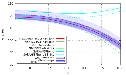
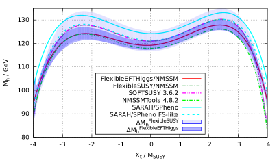
Figure 11: As Fig. 10, but for other parameter choices. We fix $M_{\text{SUSY}}=10$ TeV and $\tan\beta=5$ and plot $M_{h}$ against i) (left panel) $\lambda$, where $\kappa=\lambda$, $X_{t}=0$ and ii) (right panel) $X_{t}$ where $\kappa=\lambda=0.01$.

The left panel of Figure 11 confirms that FlexibleEFTHiggs and the fixed-order calculations in FlexibleSUSY and SOFTSUSY agree remarkably well for all values of $\lambda$ and $\kappa$, indicating that these couplings do not disrupt this remarkable numerical cancellation amongst the 3-loop logs, which yield results close to the correct ones calculated using effective field theory techniques. The same cancellation does not take place in the NMSSMTools calculation and the deviation between this result and fixed-order FlexibleSUSY gives an indication of the large uncertainty in these approaches. By contrast the right panel of Figure 11 shows that as with the MSSM, this cancellation depends on the value of $X_{t}$. The results here are very similar to those of the MSSM, since we are in the MSSM limit. Interestingly the fixed order calculation of NMSSMTools agrees very well with FlexibleEFTHiggs when $X_{t}\approx-\sqrt{6}M_{\text{SUSY}}$.

6 Numerical results in the E₆SSM

We now make a much bigger departure from minimality and consider an $E_{6}$ inspired model, with an extra $U(1)$ gauge symmetry and matter filling complete multiplets of the fundamental $\mathbf{27}$ representation of $E_{6}$. Specifically we consider the exceptional supersymmetric standard model (E₆SSM) [95, 96, 97] which has previously been shown to have very heavy sfermions [97, 98] making effective field theory techniques very important for accurately predicting the Higgs mass. In the past 2-loop expressions for the Higgs mass were obtained [95] by generalising MSSM [40] and NMSSM [82] results from effective field theory calculations that had been expanded to fixed 2-loop order. This was used in determining the spectrum [97, 98] and showing consistency with a $125$ GeV Higgs [99], though the accuracy was strictly limited due to the very heavy spectra. A first attempt at improving precision of calculations in the model was made when full 1-loop threshold corrections for the gauge and Yukawa couplings were calculated [100], with the top Yukawa threshold corrections having a significant impact on the Higgs mass. With SARAH the full 1-loop self energy can be calculated for the first time in FlexibleSUSY and SPheno and both include the option to use NMSSM and MSSM 2-loop corrections, though these will not be accurate when the exotic couplings are large and must be used with care. SARAH/SPheno can now calculate full fixed-order 2-loop order corrections. Finally, recently when studying the phenomenology of an $E_{6}$ inspired model [101], SusyHD was used to resum the logs and obtain the Higgs mass after matching to the MSSM at tree level.

Here we investigate the impact of FlexibleEFTHiggs on the Higgs mass. We will compare our results to the fixed-order calculations of FlexibleSUSY and also compare with SARAH/SPheno.

The E₆SSM extends the matter content of the MSSM with the following superfields:

$$\hat{H^{d}_{\alpha}} :\textstyle(\mathbf{1},\mathbf{2},-\frac{1}{2},-3), \hat{H^{u}_{\alpha}} :\textstyle(\mathbf{1},\mathbf{2},\frac{1}{2},-2), \hat{D^{x}_{i}} :\textstyle(\mathbf{3},\mathbf{1},-\frac{1}{3},-2), \hat{\overline{D^{x}_{i}}} :\textstyle(\mathbf{3},\mathbf{1},\frac{1}{3},-3),$$ (44)

$$\hat{S_{i}} :\textstyle(\mathbf{1},\mathbf{1},0,5), \hat{N_{i}^{c}} :\textstyle(\mathbf{1},\mathbf{1},0,0), \hat{H^{\prime}} :(\mathbf{1},\mathbf{2},-\frac{1}{2},2), \hat{\overline{H^{\prime}}} :(\mathbf{1},\mathbf{2},\frac{1}{2},-2),$$

where we include generation indices $i=1,2,3$ and $\alpha=1,2$ and we specify the $G_{\text{E\textsubscript{6}SSM}}=G_{\text{SM}}\times U(1)_{N}$ gauge group quantum numbers with the quantities in brackets specifically showing the $SU(3)$ representation, the $SU(2)$ representation, the $U(1)_{Y}$ charge without GUT normalization and the $U(1)_{N}$ charge also without GUT normalization.

The full $E_{6}$ superpotential is rather complicated, but with some simplifying assumptions including a $Z_{2}^{H}$ symmetry to forbid flavour changing neutral currents and a $Z_{2}^{B}$ symmetry to forbid proton decay, the superpotential can be written as [97],

$$\begin{split}\mathcal{W}_{\text{E\textsubscript{6}SSM}}&=\mathcal{W}_{\text{MSSM}}(\mu=0)+\lambda\hat{S}_{3}\hat{H}_{u}\hat{H}_{d}+\lambda_{\alpha}\hat{S}_{3}\hat{H}^{u}_{\alpha}\hat{H}^{d}_{\alpha}+\kappa_{i}\hat{S}_{3}\hat{D}^{x}_{i}\hat{D}^{x}_{i}+\mu^{\prime}\hat{\overline{H^{\prime}}}\hat{H}^{\prime}.\end{split}$$ (45)

The soft breaking Lagrangian then contains,

$$\mathcal{L}_{\text{E\textsubscript{6}SSM}}^{\mathrm{soft}} =\mathcal{L}_{\text{MSSM}}^{\mathrm{soft}}(B\mu=0)-m^{2}_{S_{i}}|S_{i}|^{2}-m^{2}_{H^{u}_{i}}|H^{u}_{i}|^{2}-m^{2}_{H^{d}_{i}}|H^{d}_{i}|^{2}-m^{2}_{H^{\prime}}|H^{\prime}|^{2}-m^{2}_{\overline{H^{\prime}}}|\overline{H^{\prime}}|^{2}$$

$$\phantom{={}}-m^{2}_{D_{i}}|D_{i}|^{2}-m^{2}_{\overline{D}_{i}}|\overline{D}_{i}|^{2}-\frac{1}{2}M_{1}^{\prime}\bar{\tilde{B}}^{\prime}\tilde{B}^{\prime}$$

$$\phantom{={}}-\left[B^{\prime}\mu^{\prime}\,{\overline{H^{\prime}}}\cdot{H^{\prime}}+T_{\lambda_{i}}S_{3}H_{i}^{d}\cdot H_{i}^{u}+T_{\kappa_{i}}S_{3}D_{i}\overline{D}_{i}+\textrm{h.c.}\right],$$ (46)

where $\tilde{B}^{\prime}$ is the gaugino superpartner of the $B^{\prime}$ gauge field, associated with the $U(1)_{N}$ gauge symmetry, and we have defined $H_{3}^{d}:=H_{d}$ and $H_{3}^{u}:=H_{u}$ to write the soft trilinear couplings more compactly. The third generation singlet $S_{3}$ and the neutral components of $H_{u}$ and $H_{d}$ doublets are the Higgs fields which develop the VEVs, $v_{s}/\sqrt{2}$, $v_{u}/\sqrt{2}$, and $v_{d}/\sqrt{2}$, respectively. In our analysis here we set the soft-breaking scalar and gaugino mass parameters and $\mu_{\text{eff}}=\lambda v_{s}/\sqrt{2}$ to $M_{\text{SUSY}}$, as defined in Eqs. (10). In addition, we fix

$$\begin{split}&(m_{s}^{2})_{\alpha\beta}(M_{\text{SUSY}})=\delta_{\alpha\beta}M_{\text{SUSY}}^{2},\quad(s=S,H^{u},H^{d})\\ &m^{2}_{H^{\prime}}(M_{\text{SUSY}})=m^{2}_{\overline{H^{\prime}}}(M_{\text{SUSY}})=M_{\text{SUSY}}^{2},\\ &m^{2}_{D_{i}}(M_{\text{SUSY}})=m^{2}_{\overline{D}_{i}}(M_{\text{SUSY}})=M_{\text{SUSY}}^{2},\quad(i=1,2,3)\\ &B^{\prime}\mu^{\prime}(M_{\text{SUSY}})=M_{\text{SUSY}}^{2},\\ &M_{1}^{\prime}(M_{\text{SUSY}})=M_{\text{SUSY}}.\end{split}$$ (47)

To ensure that the exotic quarks, the inert Higgsinos and the $Z^{\prime}$ boson all get $\overline{\text{DR}}$ masses equal to $M_{\text{SUSY}}$ we set

$$\kappa(M_{\text{SUSY}})=\lambda_{1,2}(M_{\text{SUSY}})=g_{1}^{\prime}(M_{\text{SUSY}})\frac{5}{\sqrt{20}}=\lambda(M_{\text{SUSY}}).$$ (48)

We also require that $v_{s}$ is fixed so that $\mu_{\text{eff}}=M_{\text{SUSY}}$, i.e.

$$v_{s}(M_{\text{SUSY}})=\frac{\sqrt{2}M_{\text{SUSY}}}{\lambda(M_{\text{SUSY}})}.$$ (49)

The E₆SSM-specific trilinear couplings are set to

$$\begin{split}&T_{\lambda_{3}}(M_{\text{SUSY}})=\frac{\sqrt{2}M_{\text{SUSY}}^{2}\sin\beta\cos\beta}{v_{s}},\\ &T_{\kappa_{1,2,3}}(M_{\text{SUSY}})=T_{\lambda_{1,2}}(M_{\text{SUSY}})=0.\end{split}$$ (50)

and the soft scalar Higgs masses $m_{H_{u}}^{2},m_{H_{d}}^{2},(m_{S}^{2})_{3,3}$ are fixed by the EWSB conditions. For the scans we use $\tan\beta(M_{\text{SUSY}})=5$ and $\lambda(M_{\text{SUSY}})=0.1$.

In Figure 12 one can see that the fixed-order FlexibleSUSY result is quite different from the FlexibleEFTHiggs result. In this case it seems that the cancellation between the logarithms is spoiled, due to the substantially altered RGE running between the EW scale and $M_{\text{SUSY}}$ caused by the additional colored matter which dramatically affect the RGE trajectory of $\alpha_{s}$ and then indirectly $\alpha_{t}$ through the gauge coupling contributions to the RGEs. The fact that we are shifted so far away from the cancellation is also reflected in the enhancement of the fixed-order uncertainty estimate from extracting $y_{t}$ in different ways, shown in red in the left panels. Figure 12 also shows our uncertainty estimates for FlexibleEFTHiggs in the right panels. As with the MSSM and NMSSM we can see that our estimation of the theory uncertainty (shown on the right) is not increasing significantly with $M_{\text{SUSY}}$, which is to be expected from the construction of this approach.

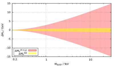
Figure 12: Higgs mass predictions and uncertainty estimates of Sec. 3 applied to the fixed-order calculations with FlexibleSUSY and to FlexibleEFTHiggs in the E₆SSM with fixed $X_{t}=0$, $\tan\beta=5$ and $\lambda=0.1$. The top row shows the Higgs mass predictions and the uncertainty estimates, the lower row only the uncertainty estimates, as in Fig. 7.

In Figure 13 we show the SARAH/SPheno prediction, along with combined uncertainty estimations for the fixed-order FlexibleSUSY and FlexibleEFTHiggs results. Here the SPheno prediction is close to the FlexibleSUSY fixed-order prediction, particularly when the top Yukawa is extracted in the same way. This should be expected since the exotic couplings are all quite small in this scenario, making the 2-loop corrections that are only in SPheno rather small. Therefore the main difference between the SPheno and FlexibleEFTHiggs results appears to be due to the resummed logs, which in this case become important at much lower $M_{\text{SUSY}}$ values. Notably at $M_{\text{SUSY}}=1$ TeV there is already a $3$ GeV gap between the FlexibleEFTHiggs prediction and the fixed-order predictions, though the results are compatible within estimated uncertainties. It is noteworthy that the estimated uncertainty of FlexibleEFTHiggs is in the range $2$–$3\,\text{GeV}$, like in the MSSM, while the one of the fixed order results has significantly increased. To improve the precision further, adding 2-loop matching to the FlexibleEFTHiggs calculation will be very important. It is also worth noting that we see no evidence of the problems due to infra-red divergences in the E₆SSM-specific SARAH/SPheno 2-loop correction here, which can be understood due to the small values of the exotic couplings.

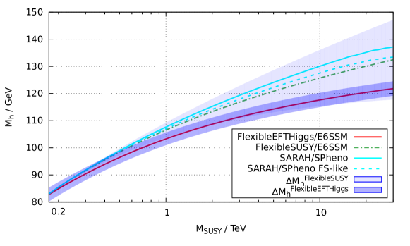
Figure 13: Predictions for $M_{h}$ and combined theoretical uncertainty estimates for FlexibleSUSY and FlexibleEFTHiggs in the E₆SSM, compared with results of other codes. We fix $X_{t}=0$, $\tan\beta=5$ and $\lambda=0.1$.

We do not investigate varying the exotic couplings here due to large dimensionality of the parameter space, but leave this for dedicated studies of this model.

7 Numerical results in the MRSSM

As another example for a non-minimal model, we study the properties of FlexibleEFTHiggs in the MRSSM, a minimal supersymmetric model with unbroken continuous R-symmetry [102]. The model is motivated in a number of ways, and particularly the mass of the SM-like Higgs boson has been shown to be compatible with experiment in a variety of parameter scenarios in Refs. [103, 104, 105]. In the following we employ the conventions of these references. The MRSSM has the same field content as the MSSM, with the following additional superfields:

$$\hat{R}_{d} :\textstyle(\mathbf{1},\mathbf{2},-\frac{1}{2}), \hat{R}_{u} :\textstyle(\mathbf{1},\mathbf{2},\frac{1}{2}), \hat{S} :\textstyle(\mathbf{1},\mathbf{1},0), \hat{T} :\textstyle(\mathbf{1},\mathbf{3},0), \hat{O} :\textstyle(\mathbf{8},\mathbf{1},0).$$ (51)

The superpotential of the MRSSM is given by

$$\begin{split}\mathcal{W}_{\text{MRSSM}}&=\mathcal{W}_{\textrm{MSSM}}(\mu=0)+\mu_{d}\hat{R}_{d}\cdot\hat{H}_{d}+\mu_{u}\hat{R}_{u}\cdot\hat{H}_{u}\\ &\phantom{={}}+\lambda_{d}\hat{S}\hat{R}_{d}\cdot\hat{H}_{d}+\lambda_{u}\hat{S}\hat{R}_{u}\cdot\hat{H}_{u}+\Lambda_{d}\hat{R}_{d}\cdot\hat{T}\hat{H}_{d}+\Lambda_{u}\hat{R}_{u}\cdot\hat{T}\hat{H}_{u}.\end{split}$$ (52)

As in the E₆SSM and $Z_{3}$-symmetric NMSSM, the $\mu$ term is forbidden in the MRSSM. New $\mu_{u,d}$ terms and Yukawa-like interactions between the $\hat{R}$ Higgs fields and $\hat{H}_{u,d}$ are allowed in general. The soft-breaking trilinear couplings as well as the Majorana mass terms for the gauginos are forbidden by the R-symmetry. The Lagrangian of the soft breaking scalar mass terms reads

$$\begin{split}\mathcal{L}_{\text{MRSSM}}^{\mathrm{soft},m^{2}}&=\mathcal{L}_{\text{MSSM}}^{\mathrm{soft}}(B\mu=T_{u}=T_{d}=T_{e}=M_{1}=M_{2}=M_{3}=0)\\ &\phantom{={}}-m_{R_{u}}^{2}\left(|R_{u}^{0}|^{2}+|R_{u}^{-}|^{2}\right)-m_{R_{d}}^{2}\left(|R_{d}^{0}|^{2}+|R_{d}^{+}|^{2}\right)\\ &\phantom{={}}-m_{S}^{2}|S|^{2}-m_{T}^{2}\left(|T^{0}|^{2}+|T^{+}|^{2}+|T^{-}|^{2}\right)-m_{O}^{2}|O|^{2}.\end{split}$$ (53)

The fermionic components of the $\hat{S}$, $\hat{T}$ and $\hat{O}$ fields mix with the gauginos $\tilde{B}$, $\tilde{W}$ and $\tilde{g}$ into Dirac fermions. The Dirac mass terms can be interpreted as being generated by the soft breaking of a supersymmetric hidden sector model via spurions. The resulting part of the soft-breaking MRSSM Langrangian reads

$$\begin{split}\mathcal{L}_{\text{MRSSM}}^{\mathrm{soft,M}}&=-M_{B}^{D}(\tilde{B}\tilde{S}-\sqrt{2}\mathcal{D}_{B}S)-M_{W}^{D}(\tilde{W}^{a}\tilde{T}^{a}-\sqrt{2}\mathcal{D}_{W}^{a}T^{a})\\ &\phantom{={}}-M_{g}^{D}(\tilde{g}^{a}\tilde{O}^{a}-\sqrt{2}\mathcal{D}_{g}^{a}O^{a})+\text{h.c.},\end{split}$$ (54)

where the auxiliary $\mathcal{D}$ fields can be eliminated by their equations of motion, giving rise to triple scalar interactions governed by the Dirac mass parameters. The Higgs fields $H_{u}$, $H_{d}$ and $S$ develop VEVs as in Eqs. (40). In addition, the electrically neutral linear combination of the Higgs triplet develops a VEV as

$$\langle T^{0}\rangle=\frac{v_{T}}{\sqrt{2}}.$$ (55)

For the MRSSM study presented in this section, we impose the boundary conditions of Eqs. (10) as well as

$$\begin{split}&m_{S}^{2}=m_{T}^{2}=m_{O}^{2}=m_{R_{d}}^{2}=m_{R_{u}}^{2}=10M_{\text{SUSY}}^{2},\\ &M_{B}^{D}=M_{W}^{D}=M_{g}^{D}=M_{\text{SUSY}},\\ &\mu_{u}=\mu_{d}=1\,\text{TeV},\tan\beta=5,\\ &\Lambda_{u}=\Lambda_{d}=-0.5,\lambda_{u}=\lambda_{d}=-0.01.\end{split}$$ (56)

at the scale $M_{\text{SUSY}}$, which is inspired by BMP3^′ from Ref. [104]. The parameters $m_{H_{u}}^{2}$, $m_{H_{d}}^{2}$, $v_{S}$, $v_{T}$ are fixed at the scale $M_{\text{SUSY}}$ by the four electroweak symmetry breaking conditions. In the fixed-order calculation, the MRSSM $\overline{\text{DR}}$ gauge and Yukawa couplings as well as the Standard Model-like vacuum expectation value $v=\sqrt{v_{u}^{2}+v_{d}^{2}}$ are calculated from the known values of $\alpha_{\text{e.m.}}^{\overline{\text{MS}},\text{SM(5)}}(M_{Z})$, $\alpha_{s}^{\overline{\text{MS}},\text{SM(5)}}(M_{Z})$, $G_{F}$, $M_{W}$, $M_{Z}$ and from the known Standard Model fermion masses at the 1-loop level at the low-energy scale $M_{Z}$. In particular, the top Yukawa coupling is calculated as described in Section 2.2, where the 2-loop SM-QCD corrections are taken into account.

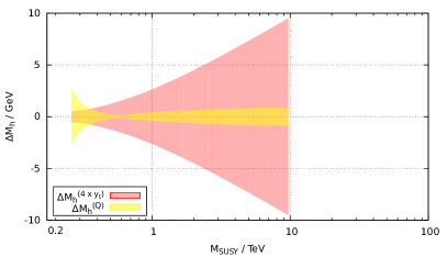
Figure 14: Uncertainty estimates of Sec. 3 for $M_{h}$, applied to the fixed-order approach with SARAH/SPheno (left panel) and to FlexibleEFTHiggs/MRSSM (right panel) as a function of $M_{\text{SUSY}}$ for the MRSSM parameter point (56).

In the left panel of Figure 14 we show the two uncertainty estimate bands for the fixed-order 2-loop calculation with SARAH/SPheno as described in Section 3.1.2:

• The yellow uncertainty band shows $\Delta M_{h}^{(Q)}$, i.e. the variation of $M_{h}$ when the renormalization scale is varied, at which $M_{h}$ is calculated. We find that for SPheno this estimation of part of the uncertainty is of the order $0.5$–$2\,\text{GeV}$ for most of the displayed $M_{\text{SUSY}}$ range, which is relatively small, because of the 2-loop Higgs mass computation. In contrast, this uncertainty is between $1$–$3\,\text{GeV}$ for FlexibleSUSY due to the missing 2-loop Higgs mass contributions.

• The red band shows $\Delta M_{h}^{(4\times y_{t})}$, i.e. the variation of $M_{h}$ in the 1-loop fixed-order calculation with FlexibleSUSY when $y_{t}^{\text{MRSSM}}$ is calculated in the four different ways presented in Section 3.1.2. As discussed, it estimates a partial theory uncertainty of the fixed-order 2-loop calculation from missing 3-loop terms. The red band would be a clear underestimation of the theory uncertainty of FlexibleSUSY’s 1-loop calculation. For both programs we find that this uncertainty estimate is dominant and can reach up to $17\,\text{GeV}$ for SUSY scales around $100\,\text{TeV}$.

In the right panel of Figure 14, the three uncertainty bands introduced in Section 3.2 for FlexibleEFTHiggs are shown:

• The turquoise uncertainty band shows $\Delta M_{h}^{(y_{t}\text{ 0L vs.\ 1L})}$, which has been obtained by calculating $y_{t}^{\text{MRSSM}}(M_{\text{SUSY}})$ using either a tree-level or a 1-loop top quark pole mass matching. For this scenario the resulting estimated uncertainty is below $0.5\,\text{GeV}$ for all values of $M_{\text{SUSY}}$. This uncertainty is smaller in the MRSSM than in the MSSM for maximal mixing, partially because $y_{t}^{\text{MRSSM}}(M_{\text{SUSY}})$ is smaller than $y_{t}^{\text{MSSM}}(M_{\text{SUSY}})$, for example $y_{t}^{\text{MRSSM},(1)}(100\,\text{TeV})=0.81$, $y_{t}^{\text{MSSM},(1)}(100\,\text{TeV})=0.87$.

• The red band shows $\Delta M_{h}^{(Q_{\text{match}})}$, i.e. the variation of $M_{h}$ when the matching scale $Q_{\text{match}}$ is varied within the interval $[M_{\text{SUSY}}/2,2M_{\text{SUSY}}]$. We find that this uncertainty is between $0.5$–$2.5\,\text{GeV}$ and thus dominates in the scenario considered here.

• The yellow band shows $\Delta M_{h}^{(Q)}$ in FlexibleEFTHiggs. This estimated uncertainty is below $2\,\text{GeV}$ for all SUSY scales above $1\,\text{TeV}$, similarly to the results in the other non-minimal SUSY models.

Based on these estimated theoretical uncertainties, we conclude that for the scenario studied here FlexibleEFTHiggs leads to a more precise prediction of $M_{h}$ than the fixed-order calculation for SUSY scales above a few TeV.

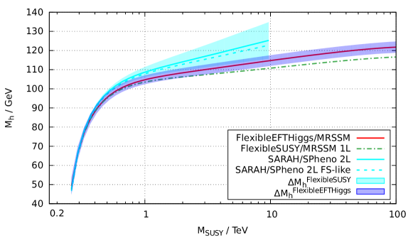
Figure 15: Predictions for $M_{h}$ and combined theoretical uncertainty estimates for FlexibleSUSY and FlexibleEFTHiggs in the MRSSM, compared with results of other codes as a function of $M_{\text{SUSY}}$ for the parameter point specified in Eqs. (56).

In Figure 15, the lightest CP-even Higgs pole mass in the MRSSM is shown as a function of $M_{\text{SUSY}}$ for the parameter point (56), together with the combined uncertainty estimates. The green dash-dotted line shows the fixed-order 1-loop calculation with FlexibleSUSY. The difference between FlexibleSUSY’s and SARAH/SPheno’s 1-loop calculations originates again from the different definition of the running top mass in the MRSSM at $M_{Z}$. The turquoise solid line shows SPheno’s fixed-order 2-loop Higgs pole mass calculation. We find that the pure 2-loop corrections enhance the Higgs mass significantly, up to $12\,\text{GeV}$ for $M_{\text{SUSY}}=10\,\text{TeV}$, compared to the 1-loop result. Such large 2-loop corrections in the $\overline{\text{DR}}$ scheme have been found and studied already in [104] and have been compared to the on-shell scheme in [107]. The turquoise dashed line again shows SPheno’s fixed-order 2-loop calculation, but using the definition (13) for the running top Yukawa coupling. We find that in this scenario all fixed-order curves become linear for $M_{\text{SUSY}}\gtrsim 1\,\text{TeV}$, which indicates that in this scenario $M_{h}$ is dominated by the leading logarithm for large SUSY scales. The red solid line shows $M_{h}$ as calculated with FlexibleEFTHiggs in the MRSSM. Since in FlexibleEFTHiggs a 1-loop Higgs mass matching and 3-loop renormalization group running is performed, FlexibleEFTHiggs resums the leading logarithmic contributions to all orders. Since FlexibleEFTHiggs resums large logarithms, and since these logarithmic contributions dominate for SUSY scales above $1\,\text{TeV}$ in this scenario, we again expect FlexibleEFTHiggs to give a more precise Higgs mass prediction for SUSY scales above a few TeV.

In addition, we show in Figure 15 the combined uncertainty estimates introduced in Section 4. In the MRSSM, SPheno is the only publicly available program which can perform a (partial) 2-loop calculation. Since $\Delta M_{h}^{\text{FlexibleSUSY}}$ is a partial estimation of missing 3-loop corrections, we can reasonably draw it only around SPheno’s 2-loop curve. The corresponding combined uncertainty for FlexibleSUSY’s 1-loop calculation is expected to be significantly larger than the shown size of $\Delta M_{h}^{\text{FlexibleSUSY}}$ and would require a separate uncertainty estimation of the missing 2-loop contributions. As expected, $\Delta M_{h}^{\text{FlexibleSUSY}}$ grows logarithmically with $M_{\text{SUSY}}$ and can be as large as $10\,\text{GeV}$ for $M_{\text{SUSY}}=10\,\text{TeV}$. In contrast, the uncertainty estimate for FlexibleEFTHiggs, $\Delta M_{h}^{\text{FlexibleEFTHiggs}}$, remains nearly constant and around $3\,\text{GeV}$ for $M_{\text{SUSY}}\gtrsim 2\,\text{TeV}$.

For comparison to the study of the 2-loop Higgs pole mass contributions in Ref. [104], we show in Table 1 the lightest CP-even Higgs pole mass in the MRSSM for the benchmark points BM1^′–BM3^′ together with combined uncertainties from Eqs. (36) and (37).

Point	SPheno	SPheno	SPheno	SPheno	FlexibleSUSY	FlexibleEFT-
	1L	2L	1L, (13)	2L, (13)	1L	Higgs 1L
BM1′	$120.4$	$125.6\pm 1.3$	$120.0$	$125.1\pm 1.3$	$120.6$	$122.1\pm 1.7$
BM2′	$120.8$	$126.0\pm 1.1$	$120.4$	$125.6\pm 1.1$	$120.2$	$121.7\pm 1.8$
BM3′	$121.0$	$125.7\pm 1.3$	$120.5$	$125.2\pm 1.3$	$120.4$	$121.9\pm 1.9$

Table 1: Lightest CP-even Higgs pole mass in GeV for the MRSSM benchmark points BM1^′–BM3^′ of Ref. [104]. The given uncertainty estimates have been obtained using Eqs. (36) and (37).

The first two data columns show $M_{h}$ calculated with SARAH and SPheno at the 1- and 2-loop level, respectively. These computations use the definition (16) to calculate $y_{t}^{\text{MRSSM}}(M_{Z})$. In the third and fourth data columns $M_{h}$ has been calculated with a modified version of SARAH/SPheno, where Eq. (13) is used to calculate $y_{t}^{\text{MRSSM}}(M_{Z})$. These different Yukawa coupling definitions amount to $0.4$–$0.5\,\text{GeV}$ shift in $M_{h}$ for these benchmark points. The fifth data column shows $M_{h}$ calculated with FlexibleSUSY at the 1-loop level, where by default Eq. (13) is used to calculate $y_{t}^{\text{MRSSM}}(M_{Z})$, and $g_{1,2}^{\text{MRSSM}}(M_{Z})$ are calculated using $M_{Z}$ and $M_{W}$ as input (instead of $M_{Z}$ and $G_{F}$ as done in SPheno). The difference between the fixed-order FlexibleSUSY and SPheno 1-loop calculations using Eq. (13) (data columns $3$ and $5$) originates from the different definitions of the electroweak gauge couplings, which affect the Higgs pole mass already at the tree-level. The last column shows the calculation of $M_{h}$ with FlexibleEFTHiggs, which resums the leading logarithms to all orders. The result of FlexibleEFTHiggs lies between the 1- and 2-loop calculations.

8 Conclusions

We have presented FlexibleEFTHiggs, an EFT calculation of the SM-like Higgs mass in any SUSY or non-SUSY model, that can make precise predictions for both high and low new physics scales. A judicious choice of matching conditions, equating pole masses, ensures that terms of $\mathcal{O}(v^{2}/M_{\text{SUSY}}^{2})$ are included, which are missed by “pure EFT” calculations such as SusyHD and FlexibleSUSY/HSSUSY. Thus large logarithms can be resummed, while ensuring that the Higgs pole mass calculation is exact at the 1-loop level. Since this choice of matching requires only self energies and tadpoles, it is also very easy to automate and apply to any SUSY (or even non-SUSY) model, where the Standard Model is the valid low energy effective field theory. This method has been implemented in FlexibleSUSY, and we have used this to obtain results in the MSSM, NMSSM, E₆SSM and MRSSM.

We discussed several ways to estimate the theoretical uncertainty of FlexibleEFTHiggs and the fixed-order approaches of FlexibleSUSY/SOFTSUSY and SPheno. These estimates show the expected behaviour, i.e. the fixed-order uncertainty rises with $M_{\text{SUSY}}$ while our FlexibleEFTHiggs estimate does not. For example in the MSSM when $M_{\text{SUSY}}$ is larger than a few TeV our combined uncertainty estimate for FlexibleEFTHiggs is smaller than our combination of various fixed-order uncertainty estimates, and similar results are obtained in the NMSSM, E₆SSM and MRSSM. Moreover, even for SUSY scales close to the EW scale we observe that the uncertainty of FlexibleEFTHiggs is around $2$–$3\,\text{GeV}$ and is thus not much larger than the fixed-order calculations, even for cases where the 2-loop contributions to the Higgs mass are large.

We also compared FlexibleEFTHiggs to other spectrum generators in all four of these models. In the MSSM we demonstrated that we understand all the differences between FlexibleEFTHiggs and SusyHD and showed that the two codes agree well at high $M_{\text{SUSY}}$ in scenarios where the 2-loop threshold corrections are negligible. In regions where the 2-loop threshold corrections are non-negligible, the codes disagree by non-logarithmic 2-loop terms, which do not increase with $M_{\text{SUSY}}$. However, in these regions the deviation of the codes lies within our uncertainty estimate for FlexibleEFTHiggs. We also found that the fixed-order calculations of FlexibleSUSY and SOFTSUSY agree surprisingly well with the EFT results of FlexibleEFTHiggs, SusyHD and FlexibleSUSY/HSSUSY even at very large $M_{\text{SUSY}}$, owing to an accidental cancellation among the 3-loop leading logarithms. This cancellation however depends on which partial 3-loop corrections are included and SPheno does not have the same tendency despite being accurate to the same formal 2-loop order as FlexibleSUSY and SOFTSUSY. This cancellation also occurs in the NMSSM, even for rather large values of the new singlet Yukawa couplings. There we see on the other hand that the full fixed-order 2-loop calculation in SARAH/SPheno is not reliable when both $M_{\text{SUSY}}$ and the exotic couplings are large, due to infrared divergences which appear in the 2-loop functions, which are not present in the other fixed order codes as they neglect these contributions.

In the E₆SSM we studied cases where all exotic couplings are rather small. Nonetheless, there is already a large impact of the exotic couplings on the fixed-order calculations at large $M_{\text{SUSY}}$ and thus we find that there is no longer good agreement between the available fixed-order calculations. The very different renormalization group flow in this model, where the $\beta$-function of $\alpha_{s}$ vanishes at 1-loop level, spoils the accidental cancellation between the 3-loop logarithms observed in the MSSM and NMSSM. We see that some of the sources of uncertainty in the fixed-order calculation, specifically the uncertainty that is estimated from different definitions of the Yukawa couplings, rises with $M_{\text{SUSY}}$ much more rapidly than in the MSSM or NMSSM. Therefore, an effective field theory calculation in this model is important presumably at lighter values of $M_{\text{SUSY}}$ than in the MSSM and NMSSM.

Finally, we applied FlexibleEFTHiggs to the MRSSM and compared the results with the available 1- and 2-loop fixed-order calculations in a scenario with sizable triplet couplings as well as with benchmark points from the literature. Similar to the E₆SSM, we find that the fixed-order programs no longer agree well with FlexibleEFTHiggs for SUSY scales above a few TeV. One of the reasons is the different running of $\alpha_{s}$ in the MRSSM, which again spoils the accidental cancellation of higher-order logarithms. We also find that the uncertainty of the fixed-order calculations, estimated by the different definitions of the top Yukawa coupling, increases more rapidly with $M_{\text{SUSY}}$ than in the MSSM or NMSSM. In contrast, the combined uncertainty estimate for FlexibleEFTHiggs is independent of $M_{\text{SUSY}}$, making the FlexibleEFTHiggs calculation more reliable already above a few TeV.

There are limitations of FlexibleEFTHiggs motivating further developments. The most obvious is the use of 1-loop matching at the SUSY scale instead of 2-loop matching. As a result, the implementation still misses 2-loop power-suppressed as well as non-power-suppressed (but non-logarithmic) terms in the Higgs pole mass. This is complementary to SARAH/SPheno, the only publicly available code that can include these 2-loop terms for all models, which can however become unreliable for large SUSY scales due to the lack of large higher-order logarithms. It is planned to extend FlexibleEFTHiggs by using the Higgs pole mass matching condition at the 2-loop level for a higher accuracy. Another possible extension of FlexibleEFTHiggs is to allow for more diverse mass hierarchies leading to additional intermediate scales at which subsets of particles are sequentially integrated out. In this way further types of potentially large logarithms can be resummed.

Appendix A Equivalence of $M_{h}$-matching to $\Delta\lambda^{(1)}$

We show the equivalence of FlexibleEFTHiggs’ matching procedure, set forth in Section 2.4, to the 1-loop threshold corrections to $\lambda$ at ${\mathcal{O}}(\alpha_{t})$ from the MSSM presented in the literature such as Eq. (10) in [44]. For this, we apply the matching condition (20) at the 1-loop level which requires that the Higgs pole mass calculated in the SM be equal to the lightest Higgs pole mass in the MSSM. In this appendix, the matching scale $Q_{\text{match}}$ shall be abbreviated to $Q$. In the Standard Model Higgs pole mass in Eq. (21), both $\Sigma^{\overline{\text{MS}},\text{SM}}_{h}$ and $t_{h}^{\overline{\text{MS}},\text{SM}}$ are evaluated at the 1-loop level. The lightest MSSM Higgs pole mass $M_{h}^{\text{MSSM}}$ is calculated at the renormalization scale $Q=M_{\text{SUSY}}$ iteratively by Eq. (17) as

$$(M_{h}^{\text{MSSM}})^{2} =(m_{h}^{\text{MSSM}})^{2}-\Sigma_{h}^{\overline{\text{DR}},\text{MSSM}}+t_{h}^{\overline{\text{DR}},\text{MSSM}}/v,$$ (57)

where $m_{h}^{\text{MSSM}}$ is the running $\overline{\text{DR}}$ Higgs mass in the MSSM, $\Sigma_{h}^{\overline{\text{DR}},\text{MSSM}}$ is the $\overline{\text{DR}}$-renormalized 1-loop self-energy of the SM-like Higgs in the MSSM, and $t_{h}^{\overline{\text{DR}},\text{MSSM}}$ is the corresponding tadpole, given by

$$\Sigma_{h}^{\overline{\text{DR}},\text{MSSM}} =c_{\alpha}^{2}\Sigma_{h_{u}h_{u}}^{\overline{\text{DR}},\text{MSSM}}+s_{\alpha}^{2}\Sigma_{h_{d}h_{d}}^{\overline{\text{DR}},\text{MSSM}}-2s_{\alpha}c_{\alpha}\Sigma_{h_{u}h_{d}}^{\overline{\text{DR}},\text{MSSM}},$$ (58)

$$\frac{t_{h}^{\overline{\text{DR}},\text{MSSM}}}{v} =c_{\alpha}^{2}\frac{t_{h_{u}}^{\overline{\text{DR}},\text{MSSM}}}{v_{u}}+s_{\alpha}^{2}\frac{t_{h_{d}}^{\overline{\text{DR}},\text{MSSM}}}{v_{d}}.$$ (59)

In the SM coupling limit, the Higgs mixing angle $\alpha$ is given by $\alpha=\beta-\frac{\pi}{2}$, and the SM-like Higgs self-energy and the tadpole become

$$\Sigma_{h}^{\overline{\text{DR}},\text{MSSM}} =s_{\beta}^{2}\Sigma_{h_{u}h_{u}}^{\overline{\text{DR}},\text{MSSM}}+c_{\beta}^{2}\Sigma_{h_{d}h_{d}}^{\overline{\text{DR}},\text{MSSM}}+2s_{\beta}c_{\beta}\Sigma_{h_{u}h_{d}}^{\overline{\text{DR}},\text{MSSM}},$$ (60)

$$\frac{t_{h}^{\overline{\text{DR}},\text{MSSM}}}{v} =s_{\beta}^{2}\frac{t_{h_{u}}^{\overline{\text{DR}},\text{MSSM}}}{v_{u}}+c_{\beta}^{2}\frac{t_{h_{d}}^{\overline{\text{DR}},\text{MSSM}}}{v_{d}}.$$ (61)

Keeping only the ${\mathcal{O}}(y_{t}^{n})$ terms, the 1-loop corrections to the SM-like Higgs in the MSSM is given by

$$-\Sigma_{h}^{\overline{\text{DR}},\text{MSSM}}+t_{h}^{\overline{\text{DR}},\text{MSSM}}/v=-\Sigma_{h}^{\overline{\text{MS}},\text{SM}}+t_{h}^{\overline{\text{MS}},\text{SM}}/v$$

$$\qquad\qquad-\frac{3(y_{t}^{\text{SM}})^{2}}{(4\pi)^{2}}\Big{\{}X_{t}^{2}c_{2\theta}^{2}B_{0}(p^{2},m_{\tilde{t}_{1}}^{2},m_{\tilde{t}_{2}}^{2})$$

$$\qquad\qquad\qquad+2\left(m_{t}+s_{2\theta}X_{t}/2\right)^{2}\left[B_{0}(p^{2},m_{\tilde{t}_{1}}^{2},m_{\tilde{t}_{1}}^{2})+B_{0}(p^{2},m_{\tilde{t}_{2}}^{2},m_{\tilde{t}_{2}}^{2})\right]$$

$$\qquad\qquad\qquad-\frac{X_{t}s_{2\theta}}{2m_{t}}\left[A_{0}(m_{\tilde{t}_{1}}^{2})+A_{0}(m_{\tilde{t}_{2}}^{2})\right]\Big{\}},$$ (62)

where $\theta$ is the stop mixing angle as defined in Eq. (19) of Ref. [9] and $s_{2\theta}=\sin 2\theta$, $c_{2\theta}=\cos 2\theta$, $X_{t}=A_{t}-\mu/\tan\beta$, $m_{t}=y_{t}^{\text{SM}}v/\sqrt{2}$. The MSSM top quark Yukawa coupling has been replaced by the corresponding SM Yukawa coupling using the tree-level relation $y_{t}^{\text{MSSM}}=y_{t}^{\text{SM}}/s_{\beta}$. By making use of the relation

$$\sin 2\theta=\frac{2m_{t}X_{t}}{m_{\tilde{t}_{1}}^{2}-m_{\tilde{t}_{2}}^{2}},$$ (63)

and inserting Eq. (62) into (20), one obtains the running Higgs mass in the Standard Model as

$$(m_{h}^{\text{SM}})^{2} =(m_{h}^{\text{MSSM}})^{2}+\Delta m_{h}^{2},$$ (64)

with the 1-loop correction

$$(4\pi)^{2}\Delta m_{h}^{2} =-3X_{t}^{2}(y_{t}^{\text{SM}})^{2}\Bigg{\{}\frac{2(y_{t}^{\text{SM}})^{2}v^{2}\left[B_{0}(p^{2},m_{\tilde{t}_{1}}^{2},m_{\tilde{t}_{1}}^{2})-B_{0}(p^{2},m_{\tilde{t}_{2}}^{2},m_{\tilde{t}_{2}}^{2})\right]}{m_{\tilde{t}_{1}}^{2}-m_{\tilde{t}_{2}}^{2}}$$

$$\phantom{={}}\qquad\qquad\qquad+B_{0}(p^{2},m_{\tilde{t}_{1}}^{2},m_{\tilde{t}_{2}}^{2})+\frac{A_{0}(m_{\tilde{t}_{2}}^{2})-A_{0}(m_{\tilde{t}_{1}}^{2})}{m_{\tilde{t}_{1}}^{2}-m_{\tilde{t}_{2}}^{2}}\Bigg{\}}$$

$$\phantom{={}}-\frac{3X_{t}^{4}(y_{t}^{\text{SM}})^{4}v^{2}}{(m_{\tilde{t}_{1}}^{2}-m_{\tilde{t}_{2}}^{2})^{2}}\Big{[}B_{0}(p^{2},m_{\tilde{t}_{1}}^{2},m_{\tilde{t}_{1}}^{2})+B_{0}(p^{2},m_{\tilde{t}_{2}}^{2},m_{\tilde{t}_{2}}^{2})-2B_{0}(p^{2},m_{\tilde{t}_{1}}^{2},m_{\tilde{t}_{2}}^{2})\Big{]}$$

$$\phantom{={}}-3(y_{t}^{\text{SM}})^{4}v^{2}\Big{[}B_{0}(p^{2},m_{\tilde{t}_{1}}^{2},m_{\tilde{t}_{1}}^{2})+B_{0}(p^{2},m_{\tilde{t}_{2}}^{2},m_{\tilde{t}_{2}}^{2})\Big{]}.$$ (65)

By inserting the stop masses in terms of the soft-breaking parameters and $X_{t}$,

$$m_{\tilde{t}_{1,2}}^{2} =m_{t}^{2}+\frac{1}{2}\left(m_{Q_{3}}^{2}+m_{U_{3}}^{2}\mp\sqrt{\left(m_{Q_{3}}^{2}-m_{U_{3}}^{2}\right)^{2}+4(m_{t}X_{t})^{2}}\right),$$ (66)

evaluating the $B_{0}$ functions at the momentum $p^{2}=\lambda v^{2}$, and expanding in powers of $v^{2}/M_{\text{SUSY}}^{2}$ up to ${\mathcal{O}}(v^{2}/M_{\text{SUSY}}^{2})$, one obtains at ${\mathcal{O}}(y_{t}^{4})$

$$\frac{(4\pi)^{2}}{(y_{t}^{\text{SM}})^{4}v^{2}}\Delta m_{h}^{2}=3\ln\frac{m_{Q_{3}}^{2}}{Q^{2}}+3\ln\frac{m_{U_{3}}^{2}}{Q^{2}}-\frac{p^{2}\left(m_{Q_{3}}^{2}+m_{U_{3}}^{2}\right)}{2m_{Q_{3}}^{2}m_{U_{3}}^{2}}$$

$$\quad\quad+X_{t}^{2}\Bigg{[}\frac{6\ln\frac{m_{Q_{3}}^{2}}{m_{U_{3}}^{2}}}{m_{Q_{3}}^{2}-m_{U_{3}}^{2}}$$

$$\quad\quad\quad\quad\quad\quad+\frac{p^{2}}{m_{Q_{3}}^{2}m_{U_{3}}^{2}\left(m_{Q_{3}}^{2}-m_{U_{3}}^{2}\right)^{3}}\Big{(}m_{Q_{3}}^{6}-6m_{Q_{3}}^{4}m_{U_{3}}^{2}+6m_{Q_{3}}^{2}m_{U_{3}}^{4}$$

$$\quad\quad\quad\quad\quad\quad\quad\quad+\frac{3}{2}m_{Q_{3}}^{2}m_{U_{3}}^{2}\left(m_{Q_{3}}^{2}+m_{U_{3}}^{2}\right)\ln\frac{m_{Q_{3}}^{2}}{m_{U_{3}}^{2}}-m_{U_{3}}^{6}\Big{)}\Bigg{]}$$

$$\quad\quad+X_{t}^{4}\Bigg{\{}-\frac{3\left[\left(m_{Q_{3}}^{2}+m_{U_{3}}^{2}\right)\ln\frac{m_{Q_{3}}^{2}}{m_{U_{3}}^{2}}-2m_{Q_{3}}^{2}+2m_{U_{3}}^{2}\right]}{\left(m_{Q_{3}}^{2}-m_{U_{3}}^{2}\right)^{3}}$$

$$\quad\quad\quad\quad\quad\quad+\frac{p^{2}}{2m_{Q_{3}}^{2}m_{U_{3}}^{2}\left(m_{Q_{3}}^{2}-m_{U_{3}}^{2}\right)^{5}}\Bigg{[}-m_{Q_{3}}^{8}+17m_{Q_{3}}^{6}m_{U_{3}}^{2}-17m_{Q_{3}}^{2}m_{U_{3}}^{6}$$

$$\quad\quad\quad\quad\quad\quad\quad\quad+3m_{Q_{3}}^{2}m_{U_{3}}^{2}\left(m_{Q_{3}}^{4}+8m_{Q_{3}}^{2}m_{U_{3}}^{2}+m_{U_{3}}^{4}\right)\ln\left(\frac{m_{U_{3}}^{2}}{m_{Q_{3}}^{2}}\right)+m_{U_{3}}^{8}\Bigg{]}\Bigg{\}}.$$ (67)

Using the relations

$$(m_{h}^{\text{SM}})^{2} =\lambda v^{2},$$ (68)

$$(m_{h}^{\text{MSSM}})^{2} =\frac{1}{4}(g_{Y}^{2}+g_{2}^{2})(v_{u}^{2}+v_{d}^{2})c_{2\beta}^{2},$$ (69)

and exploiting that $\Delta m_{h}^{2}=v^{2}\Delta\lambda$ at the 1-loop ${\mathcal{O}}(y_{t}^{4})$, one obtains from Eq. (64) in the limit $p^{2}\rightarrow 0$

$$\lambda =\frac{1}{4}(g_{Y}^{2}+g_{2}^{2})c_{2\beta}^{2}+\Delta\lambda^{(1)}$$ (70)

with

$$(4\pi)^{2}\Delta\lambda^{(1)} =3(y_{t}^{\text{SM}})^{4}\left(\ln\frac{m_{Q_{3}}^{2}}{Q^{2}}+\ln\frac{m_{U_{3}}^{2}}{Q^{2}}\right)+\frac{6(y_{t}^{\text{SM}})^{4}X_{t}^{2}\ln\frac{m_{Q_{3}}^{2}}{m_{U_{3}}^{2}}}{m_{Q_{3}}^{2}-m_{U_{3}}^{2}}$$

$$\phantom{={}}-\frac{3(y_{t}^{\text{SM}})^{4}X_{t}^{4}\left[\left(m_{Q_{3}}^{2}+m_{U_{3}}^{2}\right)\ln\frac{m_{Q_{3}}^{2}}{m_{U_{3}}^{2}}-2m_{Q_{3}}^{2}+2m_{U_{3}}^{2}\right]}{\left(m_{Q_{3}}^{2}-m_{U_{3}}^{2}\right)^{3}},$$ (71)

which is equivalent to the ${\mathcal{O}}(y_{t}^{4})$ terms of Eq. (10) of Ref. [44]. We conclude that in the MSSM FlexibleEFTHiggs’ approach is equivalent to the 1-loop threshold corrections to $\lambda$ from Ref. [44] in the SM coupling limit $\alpha=\beta-\frac{\pi}{2}$ and $p^{2}\ll M_{\text{SUSY}}^{2}$.

Appendix B Leading logarithms in the EFT, FlexibleSUSY, and SPheno-calculations

Here we derive the leading $L$-loop logarithms of the form $t_{S}\equiv\ln(M_{\text{SUSY}}/M_{t})$ governed by the two most important couplings $\alpha_{s}=g_{3}^{2}/4\pi$ and $y_{t}$, which are contained in the MSSM Higgs mass calculations in FlexibleSUSY and SPheno. We compare them to the correct leading logarithms, which are contained in the EFT calculation. For simplicity we work in the approximation of large $\tan\beta$ and identify $\sin\beta=1$, $v_{u}=v$ in the definition of the MSSM top Yukawa coupling. In the present section, we use the following notation for the required running couplings in the SM and MSSM at scale $t\equiv\ln(Q/M_{t})$:

SM: $${g}_{3}(t), y_{t}(t), v(t), \lambda(t);$$ (72)

MSSM: $$\tilde{g}_{3}(t), \tilde{y}_{t}(t), \tilde{v}(t).$$ (73)

As an abbreviation, we write the quantities at the top-mass scale and the SUSY scale as

SM, low: $$\hat{g}_{3} ={g}_{3}(0), \hat{y}_{t} =y_{t}(0), \hat{v} =v(0), \hat{\lambda} ={\lambda}(0);$$ (74)

SM, high: $${g}_{3} ={g}_{3}(t_{S}), y_{t} =y_{t}(t_{S}), v =v(t_{S}), {\lambda} ={\lambda}(t_{S});$$ (75)

MSSM, low: $$\bar{g}_{3} =\tilde{g}_{3}(0), \bar{y}_{t} =\tilde{y}_{t}(0), \bar{v} =\tilde{v}(0);$$ (76)

MSSM, high: $$\tilde{g}_{3} =\tilde{g}_{3}(t_{S}), \tilde{y}_{t} =\tilde{y}_{t}(t_{S}), \tilde{v} =\tilde{v}(t_{S}).$$ (77)

The relevant $\beta$ functions are the 1-loop $\beta$ functions for these parameters, $\beta_{X}(t)\equiv\frac{dX(t)}{dt}$. The relevant terms can be written as

$$\beta_{{g}_{3}}(t) =\beta_{{g}_{3},{g}_{3}^{2}}{g}_{3}^{3}(t), \beta_{y_{t}}(t) =y_{t}(t)\left(\beta_{y_{t},{g}_{3}^{2}}{g}_{3}^{2}(t)+\beta_{y_{t},y_{t}^{2}}y_{t}^{2}(t)\right),$$ (78)

$$\beta_{v}(t) =\beta_{v,y_{t}^{2}}v(t)y_{t}^{2}(t), \beta_{{\lambda}}(t) =\beta_{{\lambda},y_{t}^{4}}y_{t}^{4}(t)+\beta_{{\lambda},y_{t}^{2}{\lambda}}y_{t}^{2}(t){\lambda}(t)+\beta_{{\lambda},{\lambda}^{2}}{\lambda}^{2}(t)\,.$$

The values of the appearing coefficients depend on the model. In the SM, they read

$$\beta_{{g}_{3},{g}_{3}^{2}} =-7\kappa_{L}, \beta_{y_{t},{g}_{3}^{2}} =-8\kappa_{L}, \beta_{y_{t},y_{t}^{2}} =\frac{9}{2}\kappa_{L}, \beta_{v,y_{t}^{2}} =-{3}\kappa_{L},$$ (79)

$$\beta_{{\lambda},y_{t}^{4}} =-12\kappa_{L}, \beta_{{\lambda},y_{t}^{2}{\lambda}} =12\kappa_{L}, \beta_{{\lambda},{\lambda}^{2}} =12\kappa_{L}.$$

Here we use the common loop factor constant $\kappa_{L}=1/(16\pi^{2})$. In the MSSM, we denote the corresponding coefficients with a tilde; their values are

$$\tilde{\beta}_{{g}_{3},{g}_{3}^{2}} =-{3}\kappa_{L}, \tilde{\beta}_{y_{t},{g}_{3}^{2}} =-\frac{16}{3}\kappa_{L}, \tilde{\beta}_{y_{t},y_{t}^{2}} =6\kappa_{L}, \tilde{\beta}_{v,y_{t}^{2}} =-{3}\kappa_{L}.$$ (80)

As is well known, the leading logarithms can be obtained in the EFT approach by integrating the RGEs in the SM. In a first step this yields the running couplings

$${g}_{3}(t) =\sqrt{\frac{1}{\frac{1}{\hat{g}_{3}^{2}}-2\beta_{{g}_{3},{g}_{3}^{2}}t}}=\hat{g}_{3}-7t\kappa_{L}\hat{g}_{3}^{3}+\frac{147}{2}t^{2}\kappa_{L}^{2}\hat{g}_{3}^{5}-\frac{1715}{2}t^{3}\kappa_{L}^{3}\hat{g}_{3}^{7}+\ldots,$$ (81)

$$y_{t}(t) =\hat{y}_{t}+t\left(\beta_{y_{t},{g}_{3}^{2}}\hat{g}_{3}^{2}\hat{y}_{t}+\beta_{y_{t},y_{t}^{2}}\hat{y}_{t}^{3}\right)$$

$$\quad{}+\frac{1}{2}t^{2}\hat{y}_{t}\left(2\beta_{{g}_{3},{g}_{3}^{2}}\beta_{y_{t},{g}_{3}^{2}}\hat{g}_{3}^{4}+\beta_{y_{t},{g}_{3}^{2}}^{2}\hat{g}_{3}^{4}+4\beta_{y_{t},{g}_{3}^{2}}\beta_{y_{t},y_{t}^{2}}\hat{g}_{3}^{2}\hat{y}_{t}^{2}+3\beta_{y_{t},y_{t}^{2}}^{2}\hat{y}_{t}^{4}\right)+\ldots$$ (82)

$$=\hat{y}_{t}+t\kappa_{L}\left(\frac{9\hat{y}_{t}^{3}}{2}-8\hat{g}_{3}^{2}\hat{y}_{t}\right)+t^{2}\kappa_{L}^{2}\hat{y}_{t}\left(88\hat{g}_{3}^{4}-72\hat{g}_{3}^{2}\hat{y}_{t}^{2}+\frac{243}{8}\hat{y}_{t}^{4}\right)+\ldots,$$ (83)

$$v(t) =\hat{v}\left(1+\beta_{v,y_{t}^{2}}t\hat{y}_{t}^{2}+t^{2}\left(\frac{\beta_{v,y_{t}^{2}}^{2}\hat{y}_{t}^{4}}{2}+\beta_{v,y_{t}^{2}}\beta_{y_{t},{g}_{3}^{2}}\hat{g}_{3}^{2}\hat{y}_{t}^{2}+\beta_{v,y_{t}^{2}}\beta_{y_{t},y_{t}^{2}}\hat{y}_{t}^{4}\right)\right)$$ (84)

$$=\hat{v}\left(1-3t\kappa_{L}\hat{y}_{t}^{2}+t^{2}\kappa_{L}^{2}\left(24\hat{g}_{3}^{2}\hat{y}_{t}^{2}-9\hat{y}_{t}^{4}\right)\right).$$ (85)

As indicated, the running couplings on the left-hand side are taken at scale $t$, while the couplings without argument on the right-hand side are running couplings at the fixed low scale $t=0$, i.e. at $Q=M_{t}$. In a second step these results can be used to integrate the RGE for $\lambda$, to express $\hat{\lambda}$ as a function of ${\lambda}(t)$,

$$\hat{\lambda} ={\lambda}(t)-\beta_{{\lambda},y_{t}^{4}}t\hat{y}_{t}^{4}+\frac{1}{2}\beta_{{\lambda},y_{t}^{4}}t^{2}\hat{y}_{t}^{4}\left((\beta_{{\lambda},y_{t}^{2}{\lambda}}-4\beta_{y_{t},y_{t}^{2}})\hat{y}_{t}^{2}-4\beta_{y_{t},{g}_{3}^{2}}\hat{g}_{3}^{2}\right)$$

$$\quad{}-\frac{1}{6}\beta_{{\lambda},y_{t}^{4}}t^{3}\hat{y}_{t}^{4}\Big{[}(8\beta_{{g}_{3},{g}_{3}^{2}}\beta_{y_{t},{g}_{3}^{2}}+16\beta_{y_{t},{g}_{3}^{2}}^{2})\hat{g}_{3}^{4}-10\beta_{y_{t},{g}_{3}^{2}}(\beta_{{\lambda},y_{t}^{2}{\lambda}}-4\beta_{y_{t},y_{t}^{2}})\hat{g}_{3}^{2}\hat{y}_{t}^{2}$$

$$\quad\quad{}+\left(2\beta_{{\lambda},{\lambda}^{2}}\beta_{{\lambda},y_{t}^{4}}+\beta_{{\lambda},y_{t}^{2}{\lambda}}^{2}-10\beta_{{\lambda},y_{t}^{2}{\lambda}}\beta_{y_{t},y_{t}^{2}}+24\beta_{y_{t},y_{t}^{2}}^{2}\right)\hat{y}_{t}^{4}\Big{]}$$ (86)

In this equation, terms of higher-order in ${\lambda}(t)$ have been neglected. In leading-logarithmic approximation, the high-scale coupling ${\lambda}(t_{S})$ is given by matching the SM to the tree-level MSSM Higgs boson mass $m_{h}^{2}$ at the SUSY scale. The EFT prediction for the Higgs boson mass is then, in this approximation,

$$M_{h}^{2} =\hat{v}^{2}\hat{\lambda}$$ (87)

$$=m_{h}^{2}+\hat{v}^{2}\hat{y}_{t}^{4}\Big{[}12t_{S}\kappa_{L}-12t_{S}^{2}\kappa_{L}^{2}\left(16\hat{g}_{3}^{2}-3\hat{y}_{t}^{2}\right)$$

$$\quad{}+4t_{S}^{3}\kappa_{L}^{3}\left(736\hat{g}_{3}^{4}-240\hat{g}_{3}^{2}\hat{y}_{t}^{2}-99\hat{y}_{t}^{4}\right)+\ldots\Big{]}.$$ (88)

The previous equations agree with Eq. (11) from Ref. [60] and Eq. (A.17) from Ref. [42].

Now we compare these results with the leading logarithms contained in the “fixed-order” calculations. The most important difference is the definition of the Yukawa coupling. In the original FlexibleSUSY (and SOFTSUSY) or SPheno, the low-scale MSSM Yukawa coupling is defined by Eq. (13) or Eq. (16), respectively. These equations contain leading logarithms within the self energy parts $\widetilde{\Sigma}_{t}^{(1),L,R}$, and the coefficients of these logarithms is given by the difference of the SM and MSSM $\beta$ functions for the Yukawa coupling. Hence, to the leading logarithmic level, these equations imply

$$\bar{y}_{t}^{\text{$\text{FlexibleSUSY}$}} =\hat{y}_{t}\Big{[}1+\left((\beta_{y_{t},{g}_{3}^{2}}-\tilde{\beta}_{y_{t},{g}_{3}^{2}})\bar{g}_{3}^{2}+(\beta_{y_{t},y_{t}^{2}}-\tilde{\beta}_{y_{t},y_{t}^{2}})(\bar{y}_{t}^{\text{$\text{FlexibleSUSY}$}})^{2}\right)t_{S}\Big{]},$$ (89)

$$\bar{y}_{t}^{\text{$\text{SPheno}$}} =\frac{\hat{y}_{t}}{1-\left((\beta_{y_{t},{g}_{3}^{2}}-\tilde{\beta}_{y_{t},{g}_{3}^{2}})\bar{g}_{3}^{2}-(\beta_{y_{t},y_{t}^{2}}-\tilde{\beta}_{y_{t},y_{t}^{2}})(\bar{y}_{t}^{\text{$\text{SPheno}$}})^{2}\right)t_{S}},$$ (90)

which has to be iterated to find the solutions for the low-scale Yukawa couplings in terms of $\hat{y}_{t}$. The strong gauge coupling is determined by low-scale matching to the SM, but the matching condition is such that, at the leading logarithmic level, we obtain $\tilde{g}_{3}={g}_{3}$, and

$${\bar{g}_{3}^{2}} =\left[{\frac{1}{\hat{g}_{3}^{2}}-2(\beta_{{g}_{3},{g}_{3}^{2}}-\tilde{\beta}_{{g}_{3},{g}_{3}^{2}})t_{S}}\right]^{-1}.$$ (91)

The low-scale Yukawa couplings are then run up to the SUSY scale with the MSSM $\beta$ function. For the running Eq. (82) applies, with the replacement of SM by MSSM quantities. Plugging in the values of all coefficients, the final result for the SUSY-scale MSSM Yukawa couplings used in the fixed-order calculations is therefore

$$\tilde{y}_{t}^{\text{$\text{FlexibleSUSY}$}} =\hat{y}_{t}+t_{S}\kappa_{L}\left(\frac{9\hat{y}_{t}^{3}}{2}-8\hat{g}_{3}^{2}\hat{y}_{t}\right)+t_{S}^{2}\kappa_{L}^{2}\left(\frac{976\hat{g}_{3}^{4}\hat{y}_{t}}{9}-96\hat{g}_{3}^{2}\hat{y}_{t}^{3}+\frac{63\hat{y}_{t}^{5}}{2}\right)+\ldots,$$ (92)

$$\tilde{y}_{t}^{\text{$\text{SPheno}$}} =\hat{y}_{t}+t_{S}\kappa_{L}\left(\frac{9\hat{y}_{t}^{3}}{2}-8\hat{g}_{3}^{2}\hat{y}_{t}\right)+t_{S}^{2}\kappa_{L}^{2}\left(\frac{1040\hat{g}_{3}^{4}\hat{y}_{t}}{9}-88\hat{g}_{3}^{2}\hat{y}_{t}^{3}+\frac{135\hat{y}_{t}^{5}}{4}\right)+\ldots,$$ (93)

which agrees at the 1-loop level with the EFT result but disagrees at the 2-loop level. The fixed-order calculations of the MSSM Higgs boson mass then plug the SUSY-scale MSSM parameters into the $\overline{\text{DR}}$-Higgs self energy. At the leading logarithmic level, this gives

$$M_{h}^{2} =m_{h}^{2}+\tilde{v}^{2}\tilde{y}_{t}^{4}\Big{(}t_{S}c_{1}+t_{S}^{2}(c_{21}\tilde{g}_{3}^{2}+c_{22}\tilde{y}_{t}^{2})\Big{)},$$ (94)

$$c_{1} =-\beta_{{\lambda},y_{t}^{4}}=12\kappa_{L},$$ (95)

$$c_{21} =2\beta_{{\lambda},y_{t}^{4}}\beta_{y_{t},{g}_{3}^{2}}=192\kappa_{L}^{2},$$ (96)

$$c_{22} =\beta_{{\lambda},y_{t}^{4}}\left(\beta_{{\lambda},y_{t}^{2}{\lambda}}/2+2\beta_{v,y_{t}^{2}}+2\beta_{y_{t},y_{t}^{2}}\right)=-108\kappa_{L}^{2},$$ (97)

where $m_{h}$ is the running tree-level Higgs mass and where the values of the coefficients $c$ follow from the agreement of the 2-loop leading logarithms with the correct EFT result. Hence, plugging in number, we obtain the leading logarithms up to the 3-loop level, contained in the fixed-order calculations,

$$(M_{h}^{2})^{\text{$\text{FlexibleSUSY}$}} =m_{h}^{2}+\hat{v}^{2}\hat{y}_{t}^{4}\Big{[}12t_{S}\kappa_{L}-12t_{S}^{2}\kappa_{L}^{2}\left(16\hat{g}_{3}^{2}-3\hat{y}_{t}^{2}\right)$$

$$\quad{}+4t_{S}^{3}\kappa_{L}^{3}\left(\frac{736}{3}\hat{g}_{3}^{4}+144\hat{g}_{3}^{2}\hat{y}_{t}^{2}-\frac{351}{2}\hat{y}_{t}^{4}\right)\Big{]},$$ (98)

$$(M_{h}^{2})^{\text{$\text{SPheno}$}} =m_{h}^{2}+\hat{v}^{2}\hat{y}_{t}^{4}\Big{[}12t_{S}\kappa_{L}-12t_{S}^{2}\kappa_{L}^{2}\left(16\hat{g}_{3}^{2}-3\hat{y}_{t}^{2}\right)$$

$$\quad{}+4t_{S}^{3}\kappa_{L}^{3}\left(\frac{992}{3}\hat{g}_{3}^{4}+240\hat{g}_{3}^{2}\hat{y}_{t}^{2}-\frac{297}{2}\hat{y}_{t}^{4}\right)\Big{]}.$$ (99)

So far, all results are expressed in terms of low-scale SM couplings, which are connected to low-energy observables without large logarithms. It is useful to record here the equivalent results, in which these low-scale SM couplings are replaced by SUSY-scale running SM parameters, which are connected to the fundamental high-scale SUSY parameters without large logarithms. For this purpose, Eqs. (81), (83) can be inverted. The results for the high-scale Yukawa couplings used in FlexibleSUSY and SPheno are then

$$\tilde{y}_{t}^{\text{$\text{FlexibleSUSY}$}} =y_{t}+t_{S}^{2}\kappa_{L}^{2}\left(\frac{184}{9}{g}_{3}^{4}y_{t}-24{g}_{3}^{2}y_{t}^{3}+\frac{9}{8}y_{t}^{5}\right)+\ldots,$$ (100)

$$\tilde{y}_{t}^{\text{$\text{SPheno}$}} =y_{t}+t_{S}^{2}\kappa_{L}^{2}\left(\frac{248}{9}{g}_{3}^{4}y_{t}-16{g}_{3}^{2}y_{t}^{3}+\frac{27}{8}y_{t}^{5}\right)+\ldots,$$ (101)

and the results for the Higgs boson mass in the EFT, FlexibleSUSY, and SPheno are

$$(M_{h}^{2})^{\text{EFT}} =m_{h}^{2}+v^{2}y_{t}^{4}\Big{[}12t_{S}\kappa_{L}+12t_{S}^{2}\kappa_{L}^{2}\left(16{g}_{3}^{2}-9y_{t}^{2}\right)$$

$$\quad{}+4t_{S}^{3}\kappa_{L}^{3}\left(736{g}_{3}^{4}-672{g}_{3}^{2}y_{t}^{2}+90y_{t}^{4}\right)+\ldots\Big{]},$$ (102)

$$(M_{h}^{2})^{\text{$\text{FlexibleSUSY}$}} =m_{h}^{2}+v^{2}y_{t}^{4}\Big{[}12t_{S}\kappa_{L}+12t_{S}^{2}\kappa_{L}^{2}\left(16{g}_{3}^{2}-9y_{t}^{2}\right)$$

$$\quad{}+4t_{S}^{3}\kappa_{L}^{3}\left(\frac{736{g}_{3}^{4}}{3}-288{g}_{3}^{2}y_{t}^{2}+\frac{27y_{t}^{4}}{2}\right)+\ldots\Big{]},$$ (103)

$$(M_{h}^{2})^{\text{$\text{SPheno}$}} =m_{h}^{2}+v^{2}y_{t}^{4}\Big{[}12t_{S}\kappa_{L}+12t_{S}^{2}\kappa_{L}^{2}\left(16{g}_{3}^{2}-9y_{t}^{2}\right)$$

$$\quad{}+4t_{S}^{3}\kappa_{L}^{3}\left(\frac{992{g}_{3}^{4}}{3}-192{g}_{3}^{2}y_{t}^{2}+\frac{81y_{t}^{4}}{2}\right)+\ldots\Big{]}.$$ (104)

The EFT result here agrees with Ref. [42], Eq. (A.22).

References

- [1] ATLAS collaboration, G. Aad et al., Observation of a new particle in the search for the Standard Model Higgs boson with the ATLAS detector at the LHC, Phys. Lett. B716 (2012) 1–29, [1207.7214].
- [2] CMS collaboration, S. Chatrchyan et al., Observation of a new boson at a mass of 125 GeV with the CMS experiment at the LHC, Phys. Lett. B716 (2012) 30–61, [1207.7235].
- [3] P. Draper and H. Rzehak, A Review of Higgs Mass Calculations in Supersymmetric Models, Phys. Rept. 619 (2016) 1–24, [1601.01890].
- [4] S. Heinemeyer, W. Hollik and G. Weiglein, QCD corrections to the masses of the neutral CP - even Higgs bosons in the MSSM, Phys. Rev. D58 (1998) 091701, [hep-ph/9803277].
- [5] S. Heinemeyer, W. Hollik and G. Weiglein, Precise prediction for the mass of the lightest Higgs boson in the MSSM, Phys. Lett. B440 (1998) 296–304, [hep-ph/9807423].
- [6] S. Heinemeyer, W. Hollik and G. Weiglein, The Masses of the neutral CP-even Higgs bosons in the MSSM: Accurate analysis at the two loop level, Eur. Phys. J. C9 (1999) 343–366, [hep-ph/9812472].
- [7] R.-J. Zhang, Two loop effective potential calculation of the lightest CP even Higgs boson mass in the MSSM, Phys. Lett. B447 (1999) 89–97, [hep-ph/9808299].
- [8] J. R. Espinosa and R.-J. Zhang, MSSM lightest CP even Higgs boson mass to : The Effective potential approach, JHEP 03 (2000) 026, [hep-ph/9912236].
- [9] G. Degrassi, P. Slavich and F. Zwirner, On the neutral Higgs boson masses in the MSSM for arbitrary stop mixing, Nucl. Phys. B611 (2001) 403–422, [hep-ph/0105096].
- [10] J. R. Espinosa and R.-J. Zhang, Complete two loop dominant corrections to the mass of the lightest CP even Higgs boson in the minimal supersymmetric standard model, Nucl. Phys. B586 (2000) 3–38, [hep-ph/0003246].
- [11] A. Brignole, G. Degrassi, P. Slavich and F. Zwirner, On the two loop corrections to the neutral Higgs boson masses in the MSSM, Nucl. Phys. B631 (2002) 195–218, [hep-ph/0112177].
- [12] A. Dedes and P. Slavich, Two loop corrections to radiative electroweak symmetry breaking in the MSSM, Nucl. Phys. B657 (2003) 333–354, [hep-ph/0212132].
- [13] A. Brignole, G. Degrassi, P. Slavich and F. Zwirner, On the two loop sbottom corrections to the neutral Higgs boson masses in the MSSM, Nucl. Phys. B643 (2002) 79–92, [hep-ph/0206101].
- [14] A. Dedes, G. Degrassi and P. Slavich, On the two loop Yukawa corrections to the MSSM Higgs boson masses at large , Nucl. Phys. B672 (2003) 144–162, [hep-ph/0305127].
- [15] S. Heinemeyer, W. Hollik, H. Rzehak and G. Weiglein, High-precision predictions for the MSSM Higgs sector at , Eur. Phys. J. C39 (2005) 465–481, [hep-ph/0411114].
- [16] S. P. Martin, Complete two loop effective potential approximation to the lightest Higgs scalar boson mass in supersymmetry, Phys. Rev. D67 (2003) 095012, [hep-ph/0211366].
- [17] R. V. Harlander, P. Kant, L. Mihaila and M. Steinhauser, Higgs boson mass in supersymmetry to three loops, Phys. Rev. Lett. 100 (2008) 191602, [0803.0672].
- [18] P. Kant, R. V. Harlander, L. Mihaila and M. Steinhauser, Light MSSM Higgs boson mass to three-loop accuracy, JHEP 08 (2010) 104, [1005.5709].
- [19] S. Borowka, T. Hahn, S. Heinemeyer, G. Heinrich and W. Hollik, Momentum-dependent two-loop QCD corrections to the neutral Higgs-boson masses in the MSSM, Eur. Phys. J. C74 (2014) 2994, [1404.7074].
- [20] S. Borowka, T. Hahn, S. Heinemeyer, G. Heinrich and W. Hollik, Renormalization scheme dependence of the two-loop QCD corrections to the neutral Higgs-boson masses in the MSSM, Eur. Phys. J. C75 (2015) 424, [1505.03133].
- [21] G. Degrassi, S. Di Vita and P. Slavich, Two-loop QCD corrections to the MSSM Higgs masses beyond the effective-potential approximation, Eur. Phys. J. C75 (2015) 61, [1410.3432].
- [22] S. Heinemeyer, W. Hollik and G. Weiglein, FeynHiggs: A Program for the calculation of the masses of the neutral CP even Higgs bosons in the MSSM, Comput. Phys. Commun. 124 (2000) 76–89, [hep-ph/9812320].
- [23] B. C. Allanach, SOFTSUSY: a program for calculating supersymmetric spectra, Comput. Phys. Commun. 143 (2002) 305–331, [hep-ph/0104145].
- [24] A. Djouadi, J.-L. Kneur and G. Moultaka, SuSpect: A Fortran code for the supersymmetric and Higgs particle spectrum in the MSSM, Comput. Phys. Commun. 176 (2007) 426–455, [hep-ph/0211331].
- [25] B. C. Allanach, P. Athron, L. C. Tunstall, A. Voigt and A. G. Williams, Next-to-Minimal SOFTSUSY, Comput. Phys. Commun. 185 (2014) 2322–2339, [1311.7659].
- [26] P. Athron, J.-h. Park, D. Stöckinger and A. Voigt, FlexibleSUSY—A spectrum generator generator for supersymmetric models, Comput. Phys. Commun. 190 (2015) 139–172, [1406.2319].
- [27] G. Degrassi and P. Slavich, On the radiative corrections to the neutral Higgs boson masses in the NMSSM, Nucl. Phys. B825 (2010) 119–150, [0907.4682].
- [28] U. Ellwanger and C. Hugonie, NMSPEC: A Fortran code for the sparticle and Higgs masses in the NMSSM with GUT scale boundary conditions, Comput. Phys. Commun. 177 (2007) 399–407, [hep-ph/0612134].
- [29] J. Baglio, R. Gröber, M. Mühlleitner, D. T. Nhung, H. Rzehak, M. Spira et al., NMSSMCALC: A Program Package for the Calculation of Loop-Corrected Higgs Boson Masses and Decay Widths in the (Complex) NMSSM, Comput. Phys. Commun. 185 (2014) 3372–3391, [1312.4788].
- [30] P. Drechsel, L. Galeta, S. Heinemeyer and G. Weiglein, Precise Predictions for the Higgs-Boson Masses in the NMSSM, 1601.08100.
- [31] M. D. Goodsell, K. Nickel and F. Staub, Two-Loop Higgs mass calculations in supersymmetric models beyond the MSSM with SARAH and SPheno, Eur. Phys. J. C75 (2015) 32, [1411.0675].
- [32] M. Goodsell, K. Nickel and F. Staub, Generic two-loop Higgs mass calculation from a diagrammatic approach, Eur. Phys. J. C75 (2015) 290, [1503.03098].
- [33] T. Hahn, S. Heinemeyer, W. Hollik, H. Rzehak and G. Weiglein, High-Precision Predictions for the Light CP-Even Higgs Boson Mass of the Minimal Supersymmetric Standard Model, Phys. Rev. Lett. 112 (2014) 141801, [1312.4937].
- [34] H. Bahl and W. Hollik, Precise prediction for the light MSSM Higgs boson mass combining effective field theory and fixed-order calculations, 1608.01880.
- [35] R. Barbieri, M. Frigeni and F. Caravaglios, The Supersymmetric Higgs for heavy superpartners, Phys. Lett. B258 (1991) 167–170.
- [36] Y. Okada, M. Yamaguchi and T. Yanagida, Renormalization group analysis on the Higgs mass in the softly broken supersymmetric standard model, Phys. Lett. B262 (1991) 54–58.
- [37] H. E. Haber and R. Hempfling, The Renormalization group improved Higgs sector of the minimal supersymmetric model, Phys. Rev. D48 (1993) 4280–4309, [hep-ph/9307201].
- [38] J. A. Casas, J. R. Espinosa, M. Quiros and A. Riotto, The Lightest Higgs boson mass in the minimal supersymmetric standard model, Nucl. Phys. B436 (1995) 3–29, [hep-ph/9407389].
- [39] M. Carena, J. R. Espinosa, M. Quiros and C. E. M. Wagner, Analytical expressions for radiatively corrected Higgs masses and couplings in the MSSM, Phys. Lett. B355 (1995) 209–221, [hep-ph/9504316].
- [40] M. Carena, M. Quiros and C. E. M. Wagner, Effective potential methods and the Higgs mass spectrum in the MSSM, Nucl. Phys. B461 (1996) 407–436, [hep-ph/9508343].
- [41] H. E. Haber, R. Hempfling and A. H. Hoang, Approximating the radiatively corrected Higgs mass in the minimal supersymmetric model, Z. Phys. C75 (1997) 539–554, [hep-ph/9609331].
- [42] S. P. Martin, Three-loop corrections to the lightest Higgs scalar boson mass in supersymmetry, Phys. Rev. D75 (2007) 055005, [hep-ph/0701051].
- [43] P. Draper, G. Lee and C. E. M. Wagner, Precise estimates of the Higgs mass in heavy supersymmetry, Phys. Rev. D89 (2014) 055023, [1312.5743].
- [44] E. Bagnaschi, G. F. Giudice, P. Slavich and A. Strumia, Higgs Mass and Unnatural Supersymmetry, JHEP 09 (2014) 092, [1407.4081].
- [45] J. P. Vega and G. Villadoro, SusyHD: Higgs mass Determination in Supersymmetry, JHEP 07 (2015) 159, [1504.05200].
- [46] M. Binger, Higgs boson mass in split supersymmetry at two-loops, Phys. Rev. D73 (2006) 095001, [hep-ph/0408240].
- [47] G. F. Giudice and A. Strumia, Probing High-Scale and Split Supersymmetry with Higgs Mass Measurements, Nucl. Phys. B858 (2012) 63–83, [1108.6077].
- [48] G. Lee and C. E. M. Wagner, Higgs bosons in heavy supersymmetry with an intermediate mA, Phys. Rev. D92 (2015) 075032, [1508.00576].
- [49] M. Carena, J. Ellis, J. S. Lee, A. Pilaftsis and C. E. M. Wagner, CP Violation in Heavy MSSM Higgs Scenarios, JHEP 02 (2016) 123, [1512.00437].
- [50] E. Bagnaschi, F. Brümmer, W. Buchmüller, A. Voigt and G. Weiglein, Vacuum stability and supersymmetry at high scales with two Higgs doublets, JHEP 03 (2016) 158, [1512.07761].
- [51] “FlexibleSUSY Homepage.” https://flexiblesusy.hepforge.org/.
- [52] “MhEFT Homepage.” http://gabrlee.com/code.
- [53] F. Staub, SARAH, 0806.0538.
- [54] F. Staub, From Superpotential to Model Files for FeynArts and CalcHep/CompHep, Comput. Phys. Commun. 181 (2010) 1077–1086, [0909.2863].
- [55] F. Staub, Automatic Calculation of supersymmetric Renormalization Group Equations and Self Energies, Comput. Phys. Commun. 182 (2011) 808–833, [1002.0840].
- [56] F. Staub, T. Ohl, W. Porod and C. Speckner, A Tool Box for Implementing Supersymmetric Models, Comput. Phys. Commun. 183 (2012) 2165–2206, [1109.5147].
- [57] F. Staub, SARAH 3.2: Dirac Gauginos, UFO output, and more, Comput. Phys. Commun. 184 (2013) 1792–1809, [1207.0906].
- [58] F. Staub, SARAH 4 : A tool for (not only SUSY) model builders, Comput. Phys. Commun. 185 (2014) 1773–1790, [1309.7223].
- [59] M. Frank, T. Hahn, S. Heinemeyer, W. Hollik, H. Rzehak and G. Weiglein, The Higgs Boson Masses and Mixings of the Complex MSSM in the Feynman-Diagrammatic Approach, JHEP 02 (2007) 047, [hep-ph/0611326].
- [60] G. Degrassi, S. Heinemeyer, W. Hollik, P. Slavich and G. Weiglein, Towards high precision predictions for the MSSM Higgs sector, Eur. Phys. J. C28 (2003) 133–143, [hep-ph/0212020].
- [61] W. Hollik and S. Paßehr, Higgs boson masses and mixings in the complex MSSM with two-loop top-Yukawa-coupling corrections, JHEP 10 (2014) 171, [1409.1687].
- [62] W. Hollik and S. Paßehr, Two-loop top-Yukawa-coupling corrections to the charged Higgs-boson mass in the MSSM, Eur. Phys. J. C75 (2015) 336, [1502.02394].
- [63] K. Ender, T. Graf, M. Muhlleitner and H. Rzehak, Analysis of the NMSSM Higgs Boson Masses at One-Loop Level, Phys. Rev. D85 (2012) 075024, [1111.4952].
- [64] T. Graf, R. Grober, M. Muhlleitner, H. Rzehak and K. Walz, Higgs Boson Masses in the Complex NMSSM at One-Loop Level, JHEP 10 (2012) 122, [1206.6806].
- [65] M. Dugan, B. Grinstein and L. J. Hall, CP Violation in the Minimal Supergravity Theory, Nucl. Phys. B255 (1985) 413–438.
- [66] B. Allanach, C. Balazs, G. Belanger, M. Bernhardt, F. Boudjema et al., SUSY Les Houches Accord 2, Comput.Phys.Commun. 180 (2009) 8–25, [0801.0045].
- [67] L. V. Avdeev and M. Y. Kalmykov, Pole masses of quarks in dimensional reduction, Nuclear Physics B 502 (Feb., 1997) 419–435, [hep-ph/9701308].
- [68] A. Bednyakov, A. Onishchenko, V. Velizhanin and O. Veretin, Two loop MSSM corrections to the pole masses of heavy quarks, Eur.Phys.J. C29 (2003) 87–101, [hep-ph/0210258].
- [69] D. Buttazzo, G. Degrassi, P. P. Giardino, G. F. Giudice, F. Sala, A. Salvio et al., Investigating the near-criticality of the Higgs boson, JHEP 12 (2013) 089, [1307.3536].
- [70] A. V. Bednyakov, A. F. Pikelner and V. N. Velizhanin, Higgs self-coupling beta-function in the Standard Model at three loops, Nucl. Phys. B875 (2013) 552–565, [1303.4364].
- [71] J. Fleischer, F. Jegerlehner, O. V. Tarasov and O. L. Veretin, Two loop QCD corrections of the massive fermion propagator, Nucl. Phys. B539 (1999) 671–690, [hep-ph/9803493].
- [72] K. Melnikov and T. v. Ritbergen, The Three loop relation between the MS-bar and the pole quark masses, Phys. Lett. B482 (2000) 99–108, [hep-ph/9912391].
- [73] G. Degrassi, S. Di Vita, J. Elias-Miro, J. R. Espinosa, G. F. Giudice, G. Isidori et al., Higgs mass and vacuum stability in the Standard Model at NNLO, JHEP 08 (2012) 098, [1205.6497].
- [74] M. Sperling, D. Stöckinger and A. Voigt, Renormalization of vacuum expectation values in spontaneously broken gauge theories, JHEP 07 (2013) 132, [1305.1548].
- [75] M. Sperling, D. Stöckinger and A. Voigt, Renormalization of vacuum expectation values in spontaneously broken gauge theories: Two-loop results, JHEP 01 (2014) 068, [1310.7629].
- [76] U. Ellwanger, C. Hugonie and A. M. Teixeira, The Next-to-Minimal Supersymmetric Standard Model, Phys.Rept. 496 (2010) 1–77, [0910.1785].
- [77] M. Maniatis, The Next-to-Minimal Supersymmetric extension of the Standard Model reviewed, Int. J. Mod. Phys. A25 (2010) 3505–3602, [0906.0777].
- [78] J. Espinosa and M. Quiros, Two loop radiative corrections to the mass of the lightest Higgs boson in supersymmetric standard models, Phys.Lett. B266 (1991) 389–396.
- [79] J. Espinosa and M. Quiros, Upper bounds on the lightest Higgs boson mass in general supersymmetric Standard Models, Phys.Lett. B302 (1993) 51–58, [hep-ph/9212305].
- [80] T. Elliott, S. King and P. White, Supersymmetric Higgs bosons at the limit, Phys.Lett. B305 (1993) 71–77, [hep-ph/9302202].
- [81] G. Yeghian, Upper bound on the lightest Higgs mass in supersymmetric theories, Acta Phys.Slov. 49 (199) 823, [hep-ph/9904488].
- [82] U. Ellwanger and C. Hugonie, Masses and couplings of the lightest Higgs bosons in the (M+1) SSM, Eur. Phys. J. C25 (2002) 297–305, [hep-ph/9909260].
- [83] U. Ellwanger and C. Hugonie, Yukawa induced radiative corrections to the lightest Higgs boson mass in the NMSSM, Phys.Lett. B623 (2005) 93–103, [hep-ph/0504269].
- [84] U. Ellwanger, Radiative corrections to the neutral Higgs spectrum in supersymmetry with a gauge singlet, Phys.Lett. B303 (1993) 271–276, [hep-ph/9302224].
- [85] P. Pandita, Radiative corrections to the scalar Higgs masses in a nonminimal supersymmetric Standard Model, Z.Phys. C59 (1993) 575–584.
- [86] T. Elliott, S. King and P. White, Squark contributions to Higgs boson masses in the next-to-minimal supersymmetric standard model, Phys.Lett. B314 (1993) 56–63, [hep-ph/9305282].
- [87] T. Elliott, S. King and P. White, Radiative corrections to Higgs boson masses in the next-to-minimal supersymmetric Standard Model, Phys.Rev. D49 (1994) 2435–2456, [hep-ph/9308309].
- [88] F. Staub, W. Porod and B. Herrmann, The Electroweak sector of the NMSSM at the one-loop level, JHEP 1010 (2010) 040, [1007.4049].
- [89] M. D. Goodsell, K. Nickel and F. Staub, Two-loop corrections to the Higgs masses in the NMSSM, Phys.Rev. D91 (2015) 035021, [1411.4665].
- [90] M. Muhlleitner, D. T. Nhung, H. Rzehak and K. Walz, Two-Loop Contributions of the Order to the Masses of the Higgs Bosons in the CP-Violating NMSSM, JHEP 1505 (2015) 128, [1412.0918].
- [91] S. P. Martin, Three-loop Standard Model effective potential at leading order in strong and top Yukawa couplings, Phys. Rev. D89 (2014) 013003, [1310.7553].
- [92] S. P. Martin, Taming the Goldstone contributions to the effective potential, Phys. Rev. D90 (2014) 016013, [1406.2355].
- [93] J. Elias-Miro, J. R. Espinosa and T. Konstandin, Taming Infrared Divergences in the Effective Potential, JHEP 08 (2014) 034, [1406.2652].
- [94] F. Staub, P. Athron, U. Ellwanger, R. Gröber, M. Mühlleitner, P. Slavich et al., Higgs mass predictions of public NMSSM spectrum generators, Comput. Phys. Commun. 202 (2016) 113–130, [1507.05093].
- [95] S. F. King, S. Moretti and R. Nevzorov, Theory and Phenomenology of an Exceptional Supersymmetric Standard Model, Phys. Rev. D73 (2006) 035009, [hep-ph/0510419].
- [96] S. F. King, S. Moretti and R. Nevzorov, Exceptional Supersymmetric Standard Model, Phys. Lett. B634 (2006) 278–284, [hep-ph/0511256].
- [97] P. Athron, J. P. Hall, R. Howl, S. F. King, D. J. Miller, S. Moretti et al., Aspects of the Exceptional Supersymmetric Standard Model, Nucl. Phys. Proc. Suppl. 200-202 (2010) 120–129.
- [98] P. Athron, S. F. King, D. J. Miller, S. Moretti and R. Nevzorov, The Constrained Exceptional Supersymmetric Standard Model, Phys. Rev. D80 (2009) 035009, [0904.2169].
- [99] P. Athron, S. F. King, D. J. Miller, S. Moretti and R. Nevzorov, Constrained Exceptional Supersymmetric Standard Model with a Higgs Near 125 GeV, Phys. Rev. D86 (2012) 095003, [1206.5028].
- [100] P. Athron, D. Stöckinger and A. Voigt, Threshold Corrections in the Exceptional Supersymmetric Standard Model, Phys. Rev. D86 (2012) 095012, [1209.1470].
- [101] P. Athron, D. Harries, R. Nevzorov and A. G. Williams, Inspired SUSY benchmarks, dark matter relic density and a 125 GeV Higgs, Phys. Lett. B760 (2016) 19–25, [1512.07040].
- [102] G. D. Kribs, E. Poppitz and N. Weiner, Flavor in supersymmetry with an extended R-symmetry, Phys. Rev. D78 (2008) 055010, [0712.2039].
- [103] P. Dießner, J. Kalinowski, W. Kotlarski and D. Stöckinger, Higgs boson mass and electroweak observables in the MRSSM, JHEP 12 (2014) 124, [1410.4791].
- [104] P. Diessner, J. Kalinowski, W. Kotlarski and D. Stöckinger, Two-loop correction to the Higgs boson mass in the MRSSM, Adv. High Energy Phys. 2015 (2015) 760729, [1504.05386].
- [105] P. Diessner, J. Kalinowski, W. Kotlarski and D. Stöckinger, Exploring the Higgs sector of the MRSSM with a light scalar, JHEP 03 (2016) 007, [1511.09334].
- [106] D. M. Pierce, J. A. Bagger, K. T. Matchev and R.-j. Zhang, Precision corrections in the minimal supersymmetric standard model, Nucl. Phys. B491 (1997) 3–67, [hep-ph/9606211].
- [107] J. Braathen, M. D. Goodsell and P. Slavich, Leading two-loop corrections to the Higgs boson masses in SUSY models with Dirac gauginos, 1606.09213.