Dispersion relations for stationary light in one-dimensional atomic ensembles

Abstract

We investigate the dispersion relations for light coupled to one-dimensional ensembles of atoms with different level schemes. The unifying feature of all the considered setups is that the forward and backward propagating quantum fields are coupled by the applied classical drives such that the group velocity can vanish in an effect known as “stationary light”. We derive the dispersion relations for all the considered schemes, highlighting the important differences between them. Furthermore, we show that additional control of stationary light can be obtained by treating atoms as discrete scatterers and placing them at well defined positions. For the latter purpose, a multi-mode transfer matrix theory for light is developed.

I Introduction

A major quest within modern quantum optics is to obtain full control over light at the single photon level. Light is, however, highly elusive since it travels at great speed making it essential to couple light to matter to control it. A particularly promising system in that respect is an ensemble of atoms with the three-level $\Lambda$-type configuration sketched in Fig. 1(b). By applying a co-propagating classical electric field on one of the transitions, the group velocity of a quantized field resonant with the other transition can be greatly reduced compared to free-space through the process of electromagnetically induced transparency (EIT) Hau et al. (1999); Lukin (2003). By further reducing the group velocity, EIT even permits the storage of light as long lived excitations of the atoms Liu et al. (2001); Phillips et al. (2001).

EIT by itself is a linear optical effect. However, since EIT enables one to propagate electric fields near atomic resonance with low absorption, variations of EIT also constitute a popular choice for creating non-linear optical interactions at low photon numbers Harris and Hau (1999); Bajcsy et al. (2009); Gorshkov et al. (2011); Chen et al. (2013). In these setups, the relevant figure of merit is the interaction time of the photons, which is proportional to the inverse of the group velocity. For EIT, decreasing the group velocity of the polaritons (coupled light-matter excitations) simultaneously makes them increasingly atomic and less photonic in character Fleischhauer and Lukin (2000) thus also decreasing the optical non-linearity. These two effects cancel each other, which results in no enhancement of the effective non-linear interaction strength. In this context, proposals for “stationary light” have emerged as a way of creating polaritons with very small (or even vanishing) group velocities within the atomic medium, while retaining a non-zero photonic component André and Lukin (2002); Bajcsy et al. (2003). Building upon the enhanced non-linear interactions, it is in principle possible to observe the rich physics of non-linear optics at the level of a few photons Chang et al. (2008); Hafezi et al. (2012).

To use stationary light for enhancement of the non-linear interaction strength, it is essential to first understand the linear properties, which is the focus of this article. We will consider the dispersion relation for three different stationary light schemes (see Fig. 1). The dispersion relation gives the frequency (two-photon detuning) $\delta$ in terms of the Bloch vector $q$. From the dispersion relation, the group velocity $v_{\text{g}}=\dfrac{\partial{}\delta}{\partial{q}}$ can be readily obtained, and by the discussion above, it can therefore provide an intuition about how strong the non-linear interaction strength is expected to be. For the analysis, we will use two different theoretical models. The first is the continuum model, in which the atomic operators are defined for any real position coordinate $z$ between $0$ and $L$ (the total length of the ensemble). The second is the discrete model, where each atom is a linear point scatterer. The latter model is motivated by a growing interest in considering systems, where the number of atoms is relatively small, while the coupling strength and control over placement of the individual atoms are greatly improved. Examples are tapered optical fibers Le Kien et al. (2004); Vetsch et al. (2010); Goban et al. (2012) and photonic crystal waveguides Yu et al. (2014); Goban et al. (2014). In the discrete model, we find that placing the atoms in a particular way provides an additional handle for controlling the dispersion relation Witthaut and Sørensen (2010); Chang et al. (2011).

The dispersion relations for the continuum model have already been derived elsewhere Moiseev and Ham (2006); Zimmer et al. (2008); Moiseev et al. (2014). However, as we will show below, the results of the discrete model can be understood better, if they are set in context by rederiving the results of the continuum model in a different way compared to the previous publications. Additionally, even when restricted to the continuum model, treating every stationary light scheme in the same framework allows for a much easier comparison of the schemes and also for tracking the various (physically motivated) approximations that are employed in the derivations. By doing numerical calculations with the discrete model afterwards, we can test the validity of some of these approximations. We will show that for some of the stationary light schemes, the dispersion relations derived analytically using the continuum model, can also be obtained numerically as limiting cases of the discrete model with randomly placed atoms.

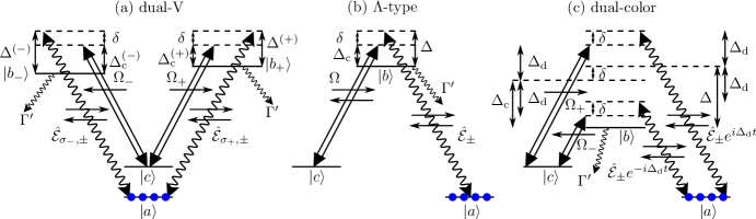
Figure 1: (Color online) Level diagrams of the three schemes that we consider. The blue circles on state $|a\rangle$ indicate that the atoms are assumed to be initialized in this state. The arrows with small wiggly lines originating on the excited states $|b_{\pm}\rangle$ and $|b\rangle$ indicate spontaneous emission with a decay rate $\Gamma^{\prime}$. The arrows between different states indicate either quantum fields (wiggly lines), or classical drives (double straight lines). The small horizontal arrows on each of these coupling arrows indicate the propagation direction. All the transitions are assumed to couple equally to both the right-moving and left-moving fields, but the arrows pointing only in a single direction on the classical drives for dual-V and dual-color schemes instead indicate that the externally applied drives propagate in the shown direction. The excited level $|b\rangle$ for the dual-color scheme is shifted vertically in order to be able to clearly show all the different detunings.

II Overview

We will consider one-dimensional ensembles of atoms with three different level and coupling schemes where stationary light can be observed (see Fig. 1). We will focus on the case of cold atoms, although for completeness we will also briefly discuss hot $\Lambda$-type atoms, which was the scheme used for the first prediction and observation of stationary light André and Lukin (2002); Bajcsy et al. (2003). Common to all stationary light schemes is the presence of two counter-propagating classical drives which couple the right-moving and left-moving modes of the quantum field through four-wave mixing Moiseev and Ham (2006). One way to explain the origin of the four-wave mixing is that an incident photon of the quantum field will be temporarily mapped to the meta-stable state $|c\rangle$ by the classical drive propagating in the same direction. The other classical drive can then retrieve this temporary excitation into a photon of the quantum field propagating in the opposite direction. In this picture, stationary light can be viewed as simultaneous EIT storage and retrieval in both the forward and backward directions Gorshkov et al. (2007a).

For the $\Lambda$-type scheme (Fig. 1(b)), a different intuitive explanation of stationary light can be given in terms of Bragg scattering. In this scheme, the two counter-propagating classical drives produce a standing wave, which modulates the refractive index of the ensemble such that it behaves as a Bragg grating. Hence, the coupling of the right-moving and left-moving modes of the quantum field happens due to the reflection of one into the other by the Bragg grating. The dynamics of the cold $\Lambda$-type scheme is, however, more complicated, which can be illustrated in terms of the allowed processes. Since both counter-propagating drives are applied on the same transition $|b\rangle\leftrightarrow|c\rangle$, it is possible for the atom to be excited by one of the classical drives and de-excited by the other. This leads to the build up of higher order Fourier components of the atomic coherence resulting in a rich and complicated physics of stationary light for cold $\Lambda$-type atoms Hansen and Mølmer (2007); Nikoghosyan and Fleischhauer (2009); Lin et al. (2009); Wu et al. (2010a, b); Peters et al. (2012). We will show that depending on the precise details of the system and the approximations used, it is possible to get dispersion relations with three different scalings close to the two-photon resonance ($\delta=0$): $\delta\propto q^{2}$ (quadratic dispersion relation of stationary light), $\delta\propto\pm q$ (EIT-like linear dispersion relation), and $\delta\propto\pm|q|^{4/3}$ Moiseev et al. (2014). In the derivations below, the first two cases will arise in the continuum model due to different truncations of the set of higher order modes of the atomic coherence. Afterwards, in the discrete model, we will show that these truncations can actually be realized physically by positioning the atoms in certain ways. The dispersion relation $\delta\propto|q|^{4/3}$ is obtained in the continuum model, when all the higher order Fourier components of the atomic coherence are summed to infinite order Moiseev et al. (2014). In the discrete model, such a scaling can be reproduced in the limit of an infinite number of randomly placed atoms.

A common trait of the two other schemes for stationary light, dual-V Zimmer et al. (2008) and dual-color Moiseev and Ham (2006) (Figs. 1(a) and 1(c) respectively) is the separation of the right-moving and left-moving fields (both classical and quantum) into different modes, either with different polarizations for dual-V or with different frequencies for dual-color. The main purpose of this separation is to suppress the higher order Fourier components of the atomic coherence since excitation and de-excitation with two different classical fields are no longer allowed. The end result of this, is that both the dual-V and dual-color schemes have quadratic dispersion relations $\delta\propto q^{2}$, just like stationary light in hot $\Lambda$-type atoms, where the higher order Fourier components of the atomic coherence are washed away by the thermal motion of the atoms André and Lukin (2002); Bajcsy et al. (2003).

Before going into the detailed derivations, we will first outline how the different scalings of the dispersion relations can arise in the continuum model for the $\Lambda$-type scheme. In the derivations below, the equations for the atoms are solved first and then substituted into the equations for the electric field. The result has the form

$$\mathinner{\left(\frac{1}{c}\mathinner{\dfrac{\partial{}}{\partial{t}}}\pm\mathinner{\dfrac{\partial{}}{\partial{z}}}\right)}\mathcal{E}_{\pm}=-in_{0}\alpha_{1}(\delta)\mathcal{E}_{\pm}-in_{0}\alpha_{2}(\delta)\mathcal{E}_{\mp},$$ (1)

where $\mathcal{E}_{\pm}$ are slowly varying (both in time and space) electric fields moving either to the right ($+$) or the left ($-$), and $\alpha_{1}$ and $\alpha_{2}$ describe the (frequency dependent) atomic polarizability. In the equation above, we have separated out the density $n_{0}$ and a factor of $-i$ for consistency with the notation below. Due to the steep dispersion of the light field, i.e., since the speed of light $c$ is large, we will omit the time derivative of the field. If we look for solutions of the form $\mathcal{E}_{\pm}(z)=\mathcal{E}_{\pm}(0){\rm e}^{iqz}$, we arrive at the coupled equations

$$\begin{pmatrix}\alpha_{1}(\delta)+\frac{q}{n_{0}}&\alpha_{2}(\delta)\\ \alpha_{2}(\delta)&\alpha_{1}(\delta)-\frac{q}{n_{0}}\end{pmatrix}\begin{pmatrix}\mathcal{E}_{+}\\ \mathcal{E}_{-}\end{pmatrix}=\begin{pmatrix}0\\ 0\end{pmatrix}.$$ (2)

To have non-trivial solutions, the determinant of the matrix in this equation must vanish, which results in the equation

$$\alpha_{1}^{2}(\delta)-\alpha_{2}^{2}(\delta)-\frac{q^{2}}{n_{0}^{2}}=0,$$ (3)

which relates $q$ and $\delta$, and thereby gives the dispersion relation.

All the situations that we consider are chosen such that they have a solution at $q=0$ and $\delta=0$ (a dark state Fleischhauer and Lukin (2000)). To fulfill Eq. (3) with $q=0$ and $\delta=0$, we must have $\alpha_{1}^{2}(0)=\alpha_{2}^{2}(0)$, and in the detailed derivation below, we will choose phases of the classical drives such that $\alpha_{1}(0)=-\alpha_{2}(0)$. We will then encounter three cases that give different scalings of the dispersion relation.

If the coefficients $\alpha_{1}(0)$ and $\alpha_{2}(0)$ are non-zero, Eq. (2) with $q=0$ will only have a single solution ($\mathcal{E}_{+}=\mathcal{E}_{-}$ for $\alpha_{1}(0)=-\alpha_{2}(0)$). In this case we can expand $\alpha_{1}(\delta)$ and $\alpha_{2}(\delta)$ to first order in the detuning to obtain

$$2\alpha_{1}(0)(\alpha_{1}^{\prime}+\alpha_{2}^{\prime})\delta=\frac{q^{2}}{n_{0}^{2}},$$ (4)

where we have chosen $\alpha_{2}(0)=-\alpha_{1}(0)$ and $\alpha_{k}^{\prime}$ denote the derivatives of $\alpha_{k}$ ($k=1,2$) at $\delta=0$. Assuming $\alpha_{1}^{\prime}+\alpha_{2}^{\prime}\neq 0$ we obtain a single solution with a quadratic dispersion relation

$$\delta\propto q^{2}.$$ (5)

This is the original stationary light dispersion relation André and Lukin (2002); Bajcsy et al. (2003) and is the typical situation encountered near an extremum of a single dispersion band. This is also the situation we will encounter for the dual-V and dual-color schemes.

If $\alpha_{1}(0)=\alpha_{2}(0)=0$ and $q=0$, the matrix in Eq. (2) has all elements equal to zero. Hence, any vector is an eigenvector of this matrix, and we can pick two orthogonal ones, which can be interpreted as two degenerate solutions. After expanding $\alpha_{1}$ and $\alpha_{2}$ in $\delta$, the lowest order contributions to $\alpha_{1}^{2}(\delta)-\alpha_{2}^{2}(\delta)$ in Eq. (3) is then quadratic resulting in

$$\mathinner{\left({\alpha^{\prime}_{1}}^{2}-{\alpha^{\prime}_{2}}^{2}\right)}\delta^{2}=\frac{q^{2}}{n_{0}^{2}}.$$ (6)

Assuming $\mathinner{\left({\alpha^{\prime}_{1}}^{2}-{\alpha^{\prime}_{2}}^{2}\right)}\neq 0$ we then obtain two solutions with a linear dispersion relation

$$\delta\propto\pm q.$$ (7)

This result reflects the fact that if two dispersion bands cross, they tend to be linear around the crossing.

The $\Lambda$-type scheme also provides an example of a different scaling of two crossing dispersion bands. It is obtained when $\alpha_{1}(0)=\alpha_{2}(0)=0$, but the functions $\alpha_{1}(\delta)$ and $\alpha_{2}(\delta)$ can not be expanded at $\delta=0$ (not analytic). This will be the case for the solution for the $\Lambda$-type scheme, when all the higher order Fourier components of the atomic coherence are accounted for. We obtain the scalings $\alpha_{1},\alpha_{2}\propto\sqrt{\delta}$, but according to Eq. (3) the dispersion relation is determined by the difference of the squares, which has the scaling $\alpha_{1}^{2}(\delta)-\alpha_{2}^{2}(\delta)\propto\delta^{3/2}$ such that we obtain

$$\delta\propto\pm|q|^{4/3}.$$ (8)

The structure of the article is as follows. In the continuum model, the dispersion relations for the three stationary light schemes are derived in Sec. III.1 (dual-V), Sec. III.2 ($\Lambda$-type), and Sec. III.3 (dual-color). For completeness, in Sec. III.4 we include a brief discussion of how the results for the dual-color scheme can provide another confirmation that the dispersion relation for hot (i.e. moving) $\Lambda$-type atoms is quadratic Peters et al. (2012). In Sec. IV, the discrete model is discussed (Sec. IV.2 for dual-V and Sec. IV.3 for $\Lambda$-type). In Sec. V, we look at the connection between the dispersion relations and scattering properties of the atomic ensembles under the conditions of stationary light.

III Continuum model

III.1 Dispersion relations for cold Dual-V atoms

The dual-V scheme as shown in Fig. 1(a) has already been studied in Ref. Zimmer et al. (2008) and was shown to have a quadratic dispersion relation. Here we do a different derivation of this result to serve as the context for the discussion of the other stationary light schemes. We take the dual-V scheme as the starting point, because the derivation of the dispersion relation is more straightforward, even if the additional atomic energy level and two different polarizations of the electric fields make the setup of the problem more complicated. In the course of the derivation we will introduce most of the definitions that we will also use for the other schemes ($\Lambda$-type and dual-color).

The atomic ensemble is assumed to be a one-dimensional medium of length $L$ consisting of $N$ atoms. In the continuum model, the atomic density $n_{0}=N/L$ is assumed to be constant throughout the length of the ensemble. The atoms are described by the collective operators

$$\hat{\sigma}_{\alpha\beta}(z)=\frac{1}{n_{0}}\sum_{j}\delta(z-z_{j})\hat{\sigma}_{\alpha\beta,j}$$ (9)

where $\hat{\sigma}_{\alpha\beta,j}=|\alpha_{j}\rangle\langle\beta_{j}|$ is the atomic coherence ($\alpha\neq\beta$) or population ($\alpha=\beta$) of atom $j$. These collective operators have the equal time commutation relations

$$[\hat{\sigma}_{\alpha\beta}(z),\hat{\sigma}_{\alpha^{\prime}\beta^{\prime}}(z^{\prime})] =\frac{1}{n_{0}}\delta(z-z^{\prime})(\delta_{\beta,\alpha^{\prime}}\hat{\sigma}_{\alpha\beta^{\prime}}-\delta_{\beta^{\prime},\alpha}\hat{\sigma}_{\alpha^{\prime}\beta}).$$ (10)

Throughout this paper, all operators are defined to be slowly-varying in time, since we work in the interaction picture relative to the carrier frequencies of the fields.

The dual-V scheme has two excited states, $|b_{+}\rangle$ and $|b_{-}\rangle$, which both couple to the ground state $|a\rangle$ but with the different polarization modes, $\sigma_{+}$ and $\sigma_{-}$, of the quantum field. The $\sigma_{+}$ mode only couples the $|a\rangle\leftrightarrow|b_{+}\rangle$ transition, and the $\sigma_{-}$ mode only couples the $|a\rangle\leftrightarrow|b_{-}\rangle$ transition. The operator for the total quantum field $\hat{\mathcal{E}}_{\sigma_{\pm}}$ for the different polarizations can be decomposed as

$$\hat{\mathcal{E}}_{\sigma_{\pm}}(z)=\hat{\mathcal{E}}_{\sigma_{\pm},+}(z)e^{ik_{0}z}+\hat{\mathcal{E}}_{\sigma_{\pm},-}(z)e^{-ik_{0}z},$$ (11)

where $k_{0}$ is the wave vector corresponding to the carrier frequency of the quantum fields $\omega_{0}$, i.e. $k_{0}=\omega_{0}/c$. For the $\sigma_{+}$ fields, $\hat{\mathcal{E}}_{\sigma_{+},+}(z)$ is the spatially slowly-varying annihilation operator at position $z$ for the field moving to the right (positive direction), and $\hat{\mathcal{E}}_{\sigma_{+},-}(z)$ is the operator for the field moving to the left (negative direction). Analogous definitions hold for the $\sigma_{-}$ fields. We will be concerned with the dynamics within a frequency interval around atomic resonances that is much smaller than the carrier frequencies of the fields. Therefore, the right-moving and left-moving quantum fields (for each polarization mode) can be regarded as being completely separate Shen and Fan (2005) with the equal time commutation relations

$$[\hat{\mathcal{E}}_{\alpha}(z),\hat{\mathcal{E}}^{\dagger}_{\beta}(z^{\prime})]=\delta_{\alpha\beta}\delta(z-z^{\prime}),$$ (12)

where $\alpha$ and $\beta$ each denote one of the four possible combinations of polarization ($\sigma_{\pm}$) and propagation direction ($\pm$).

The transition frequencies between the atomic energy levels $|\alpha\rangle$ and $|\beta\rangle$ will be denoted by $\omega_{\alpha\beta}$. The quantum fields are detuned from the atomic transition frequencies by $\Delta_{0}^{(\pm)}=\omega_{0}-\omega_{ab_{\pm}}$. The excited states $|b_{+}\rangle$ and $|b_{-}\rangle$ are assumed to have the same incoherent decay rate $\Gamma^{\prime}$ to modes other than the forward and backward propagating ones. We account for $\Gamma^{\prime}$ by making the detunings complex: $\tilde{\Delta}_{0}^{(\pm)}=\Delta_{0}^{(\pm)}+i\Gamma^{\prime}/2$. In the calculations below, we will employ Fourier transformation, where the Fourier frequencies $\omega$ will be defined relative to the carrier frequency $\omega_{0}$. For ease of notation we therefore define the detunings $\Delta^{(\pm)}=\Delta^{(\pm)}_{0}+\omega$. As opposed to the detunings of the carrier frequency $\Delta^{(\pm)}_{0}$, the detunings $\Delta^{(\pm)}$ additionally include the shift due to the finite bandwidth of the quantum field.

The two counter-propagating classical drives are in the two different polarization modes. Here, the polarization and the propagation direction are chosen such that $\Omega_{+}$ is the Rabi frequency of the $\sigma_{+}$ classical drive propagating in the positive direction that couples the transition $|b_{+}\rangle\leftrightarrow|c\rangle$, and $\Omega_{-}$ is the Rabi frequency of the $\sigma_{-}$ classical drive propagating in the negative direction that couples the transition $|b_{-}\rangle\leftrightarrow|c\rangle$. The classical drives have frequency $\omega_{\text{c}}$ and are detuned from the respective transitions by $\Delta_{\text{c}}^{(\pm)}=\omega_{\text{c}}-\omega_{b_{\pm}c}$. Furthermore, we define the two-photon detuning $\delta_{0}=\omega_{0}-\omega_{\text{c}}-\omega_{ac}$, which has a unique definition, since the quantum fields have the same carrier frequency ($\omega_{0}$) for both polarizations, and the classical drives have the same frequency ($\omega_{\text{c}}$) for both polarizations. In terms of $\Delta_{0}^{(\pm)}$ and $\Delta_{\text{c}}^{(\pm)}$ above, we also have $\delta_{0}=\Delta_{0}^{(+)}-\Delta_{\text{c}}^{(+)}=\Delta_{0}^{(-)}-\Delta_{\text{c}}^{(-)}$. Similar to $\Delta^{(\pm)}$ above, there is a complementary definition of the two-photon detning $\delta=\delta_{0}+\omega$ that takes into account the finite bandwidth of the quantum field. The wave vector of the classical drive is $k_{\text{c}}=\omega_{\text{c}}/c$, but throughout our calculations we are going to assume $k_{\text{c}}\approx k_{0}$.

The Hamiltonian for the dual-V scheme can be decomposed as $\hat{H}_{\text{V}}=\hat{H}_{\text{V,a}}+\hat{H}_{\text{V,i}}+\hat{H}_{\text{V,p}}$, where $\hat{H}_{\text{V,a}}$ describes the atoms, $\hat{H}_{\text{V,p}}$ describes the photons, and $\hat{H}_{\text{V,i}}$ describes the light-matter interactions. In the interaction picture and the rotating wave approximation, the parts are

$$\begin{aligned} \hat{H}_{\text{V,a}}=-\hbar n_{0}\int\left[\sum_{\alpha\in\mathinner{\left\{+,-\right\}}}\tilde{\Delta}_{0}^{(\alpha)}\hat{\sigma}_{b_{\alpha}b_{\alpha}}(z)+\delta_{0}\hat{\sigma}_{cc}(z)\right]\operatorname{d\!}z,\end{aligned}$$ (13a)

$$\begin{aligned} \hat{H}_{\text{V,i}}=-\hbar n_{0}\int&\sum_{\alpha\in\mathinner{\left\{+,-\right\}}}\Bigg{\{}\left[\hat{\sigma}_{b_{\alpha}c}(z)\Omega_{\alpha}e^{\alpha ik_{\text{c}}z}+\text{H.c.}\right]\\ &+g\sqrt{2\pi}\left[\hat{\sigma}_{b_{\alpha}a}(z)\hat{\mathcal{E}}_{\sigma_{\alpha}}(z)+\text{H.c.}\right]\Bigg{\}}\operatorname{d\!}z,\end{aligned}$$ (13b)

$$\begin{aligned} \hat{H}_{\text{V,p}}=-i\hbar c\int\sum_{\alpha\in\{+,-\}}\Bigg{[}&\hat{\mathcal{E}}_{\sigma_{\alpha},+}^{\dagger}(z)\mathinner{\dfrac{\partial{}\hat{\mathcal{E}}_{\sigma_{\alpha},+}(z)}{\partial{z}}}\\ &-\hat{\mathcal{E}}_{\sigma_{\alpha},-}^{\dagger}(z)\mathinner{\dfrac{\partial{}\hat{\mathcal{E}}_{\sigma_{\alpha},-}(z)}{\partial{z}}}\Bigg{]}\operatorname{d\!}z,\end{aligned}$$ (13c)

where $g=\mu\sqrt{\omega_{ab_{\pm}}/(4\pi\hbar\epsilon_{0}A)}$ (in this constant, we assume that $\omega_{ab_{+}}\approx\omega_{ab_{-}}$), $\mu$ is the matrix element of the atomic dipole, and $A$ is the effective area of the electric field mode.

The Heisenberg equations of motion for the electric field operators are given by

$$\mathinner{\left(\mathinner{\dfrac{\partial{}}{\partial{t}}}\pm c\mathinner{\dfrac{\partial{}}{\partial{z}}}\right)}\mathcal{E}_{\sigma_{+},\pm} =ig\sqrt{2\pi}n_{0}\sigma_{ab_{+}}e^{\mp ik_{0}z}.$$ (14a)

$$\mathinner{\left(\mathinner{\dfrac{\partial{}}{\partial{t}}}\pm c\mathinner{\dfrac{\partial{}}{\partial{z}}}\right)}\mathcal{E}_{\sigma_{-},\pm} =ig\sqrt{2\pi}n_{0}\sigma_{ab_{-}}e^{\mp ik_{0}z}.$$ (14b)

Here and in the following we will omit the hats above the operators as soon as the Heisenberg equations of motion are found, since we will be considering linear effects for which the operator character does not play any role. The noise operators, normally included in the Heisenberg equations of motion whenever incoherent losses are present ($\Gamma^{\prime}>0$), are also omitted, since they can be shown to not have any effect Zimmer et al. (2008); Gorshkov et al. (2007b, a). The equations of motion for the atoms are found under the assumption that the probe field is weak and that the ensemble is initially prepared in the ground state. Hence, we set $\hat{\sigma}_{aa}\approx 1$, $\hat{\sigma}_{b_{\pm}b_{\pm}}\approx\hat{\sigma}_{b_{\pm}b_{\mp}}\approx\hat{\sigma}_{cc}\approx\hat{\sigma}_{b_{\pm}c}\approx 0$, and get the equations

$$\mathinner{\dfrac{\partial{}\sigma_{ab_{\pm}}}{\partial{t}}}=i\tilde{\Delta}_{0}^{(\pm)}\sigma_{ab_{\pm}}+i\Omega_{\pm}\sigma_{ac}e^{\pm ik_{\text{c}}z}+ig\sqrt{2\pi}\mathcal{E}_{\sigma_{\pm}},$$ (15a)

$$\mathinner{\dfrac{\partial{}\sigma_{ac}}{\partial{t}}}=i\delta_{0}\sigma_{ac}+i\Omega_{+}^{*}\sigma_{ab_{+}}e^{-ik_{\text{c}}z}+i\Omega_{-}^{*}\sigma_{ab_{-}}e^{ik_{\text{c}}z}.$$ (15b)

We note that it is in Eqs. (15) that the continuum approximation is first applied, since both the Hamiltonian (13) and Eqs. (14) in principle retain the discrete nature of the atoms due to the definition (9). Eqs. (15) are derived under the approximation $\sigma_{aa}\approx 1$, which can be viewed as two separate approximations. The first is that $\sigma_{aa,j}\approx 1$ for all the individual atoms $j$. Together with the definition (9), we see that $\sigma_{aa}\approx 1$ also means approximating $\sum_{j}\delta(z-z_{j})\approx n_{0}$, and this is what we mean by the continuum approximation. In the analysis done in Ref. Sørensen and Sørensen (2008) it was shown in a perturbative calculation that this is a good approximation for randomly placed atoms. Using the discrete model in Sec. IV below, we will verify it explicitly without any perturbative assumptions.

We make two assumptions for simplicity and to be able to relate this derivation to the secular approximation for $\Lambda$-type atoms, which we discuss below. First, we assume equal atomic transition frequencies, $\omega_{b_{+}c}=\omega_{b_{-}c}$, so that ${\Delta_{0}^{(+)}=\Delta_{0}^{(-)}=\Delta_{0}}$, and ${\Delta_{\text{c}}^{(+)}=\Delta_{\text{c}}^{(-)}=\Delta_{\text{c}}}$. Second, we assume equal classical drive strengths, $\Omega_{+}=\Omega_{-}=\Omega_{0}/2$.

With the above assumptions and defining the slowly-varying versions of $\sigma_{ab\pm}$ by

$$\sigma_{ab}^{\pm}=\sigma_{ab\pm}e^{\mp ik_{0}z},$$ (16)

the equations of motion become

$$\mathinner{\dfrac{\partial{}\sigma_{ab}^{\pm}}{\partial{t}}}=i\tilde{\Delta}_{0}\sigma_{ab}^{\pm}+i\frac{\Omega_{0}}{2}\sigma_{ac}+ig\sqrt{2\pi}\mathcal{E}_{\sigma_{\pm}}e^{\mp ik_{0}z},$$ (17a)

$$\mathinner{\dfrac{\partial{}\sigma_{ac}}{\partial{t}}}=i\delta_{0}\sigma_{ac}+i\frac{\Omega_{0}^{*}}{2}(\sigma_{ab}^{+}+\sigma_{ab}^{-}),$$ (17b)

and after the Fourier transform in time,

$$0=i\tilde{\Delta}\sigma_{ab}^{\pm}+i\frac{\Omega_{0}}{2}\sigma_{ac}+ig\sqrt{2\pi}\mathcal{E}_{\sigma_{\pm}}e^{\mp ik_{0}z},$$ (18a)

$$0=i\delta\sigma_{ac}+i\frac{\Omega_{0}^{*}}{2}(\sigma_{ab}^{+}+\sigma_{ab}^{-}).$$ (18b)

Here, we have absorbed the Fourier frequency variable $\omega$ into the detunings by defining $\tilde{\Delta}=\tilde{\Delta}_{0}+\omega$ and $\delta=\delta_{0}+\omega$. Isolating $\sigma_{ac}$ from Eq. (18b) and inserting into Eqs. (18a) gives two coupled equations

$$0=\left(1-\frac{\delta_{\text{S}}}{2\delta}\right)\sigma_{ab}^{\pm}-\frac{\delta_{\text{S}}}{2\delta}\sigma_{ab}^{\mp}+\frac{g\sqrt{2\pi}}{\tilde{\Delta}}\mathcal{E}_{\sigma_{\pm}}e^{\mp ik_{0}z}.$$ (19)

Here, we have introduced

$$\delta_{\text{S}}=\frac{|\Omega_{0}|^{2}}{2\tilde{\Delta}}.$$ (20)

For $\delta,\Gamma^{\prime}\ll\Delta_{\text{c}}$, $\delta_{\text{S}}\approx|\Omega_{0}|^{2}/(2\Delta_{\text{c}})$ is the total AC Stark shift induced by the classical drives on the state $|c\rangle$. We will focus on the case when $|\delta|\ll|\delta_{\text{S}}|$. For ${|\delta|\gtrsim|\delta_{\text{S}}|}$, the frequency is outside the scale of the strongest effect induced by the classical drives. Therefore, the dispersion relations for the different schemes all cross over to the dispersion relation corresponding to a two-level atom, as can be seen in Fig. 2.

Figure 2: (Color online) Log-log plot of the dispersion relations for the different setups. The upper solid black curve is for EIT (see Eq. (37)). The lower solid red curve is the quadratic dispersion relation for the dual-V setup (or the secular approximation for the $\Lambda$-type scheme) given by Eq. (31). The dashed green curves are the dispersion relations for the truncations of Eqs. (41) with increasing number of the Fourier components of $\sigma_{ab}$ and $\sigma_{ac}$. The dispersion relations for small $\text{Re}[q]/n_{0}$ alternate between linear and quadratic depending on the truncation. The solid blue curve is the analytical limit of these dispersion relations given by Eq. (56). The lower dashed cyan curve is for the dual-color scheme with $\Delta_{\text{d}}/\Gamma=1$. It overlaps the quadratic dual-V curve, so that the difference is not visible. The common parameters for all the curves are $\Gamma_{\text{1D}}/\Gamma=0.1$, $\Delta_{\text{c}}/\Gamma=-90$, and $\Omega_{0}/\Gamma=1$. The curves are obtained by using a real $\delta$, calculating complex $q$ and then plotting $\delta/\Gamma$ as a function of $\text{Re}[q]/n_{0}$. The alternative approach: using real $q$, calculating complex $\delta$ and then plotting $\text{Re}[\delta]/\Gamma$ as a function of $q/n_{0}$ will produce results that are indistinguishable for this parameter regime (big $\Delta_{\text{c}}/\Gamma$ and $\Delta_{\text{d}}/|\delta_{\text{S}}|$). For all the dispersion relations we pick the branches such that $\text{Re}[q]/n_{0}>0$.

Solving Eqs. (19), we find

$$\begin{aligned} \sigma_{ab}^{\pm}=-\frac{g\sqrt{2\pi}}{\tilde{\Delta}}\Bigg{[}&\frac{\delta-\delta_{\text{S}}/2}{\delta-\delta_{\text{S}}}\mathcal{E}_{\sigma_{\pm}}e^{\mp ik_{0}z}\\ &+\frac{\delta_{\text{S}}/2}{\delta-\delta_{\text{S}}}\mathcal{E}_{\sigma_{\mp}}e^{\pm ik_{0}z}\Bigg{]}.\end{aligned}$$ (21)

We insert Eqs. (21) into the Fourier transformed versions of Eqs. (14) and remove terms with rapid spatial variation, i.e. terms containing factors $e^{ink_{0}z}$ with the integer $n$ fulfilling $|n|>0$. As a consequence, $\mathcal{E}_{\sigma_{+},+}$ and $\mathcal{E}_{\sigma_{-},-}$ form a closed set of equations, separate from $\mathcal{E}_{\sigma_{+},-}$ and $\mathcal{E}_{\sigma_{-},+}$. We therefore find

$$\begin{aligned} &\mathinner{\left(-i\frac{\omega}{cn_{0}}\pm\frac{1}{n_{0}}\mathinner{\dfrac{\partial{}}{\partial{z}}}\right)}\mathcal{E}_{\sigma_{\pm},\pm}\\ &=-i\frac{\Gamma_{\text{1D}}}{2\tilde{\Delta}}\left[\frac{\delta-\delta_{\text{S}}/2}{\delta-\delta_{\text{S}}}\mathcal{E}_{\sigma_{\pm},\pm}+\frac{\delta_{\text{S}}/2}{\delta-\delta_{\text{S}}}\mathcal{E}_{\sigma_{\mp},\mp}\right],\end{aligned}$$ (22a)

$$\begin{aligned} &\mathinner{\left(-i\frac{\omega}{cn_{0}}\mp\frac{1}{n_{0}}\mathinner{\dfrac{\partial{}}{\partial{z}}}\right)}\mathcal{E}_{\sigma_{\pm},\mp}=-i\frac{\Gamma_{\text{1D}}}{2\tilde{\Delta}}\frac{\delta-\delta_{\text{S}}/2}{\delta-\delta_{\text{S}}}\mathcal{E}_{\sigma_{\pm},\mp},\end{aligned}$$ (22b)

where we have introduced the decay rate $\Gamma_{\text{1D}}=4\pi g^{2}/c$ which describes the photon emission rate into the one-dimensional modes (the sum of right-moving and left-moving) from the atoms. The total decay rate of an excited atom is then $\Gamma=\Gamma^{\prime}+\Gamma_{\text{1D}}$. In the absence of inhomogeneous broadening, the decay rate $\Gamma_{\text{1D}}$ is related to the resonant optical depth $d_{\text{opt}}$ through $d_{\text{opt}}=2N\Gamma_{\text{1D}}/\Gamma$.

Since the Hamiltonian (13) is periodic in space with period $2\pi/k_{0}$ we can invoke Bloch’s theorem and look for solutions to Eqs. (22) of the form

$$\mathcal{E}_{\sigma_{\pm}}(z,\omega)=\mathinner{\left(\mathcal{E}_{\sigma_{\pm},+}(0,\omega)e^{ik_{0}z}+\mathcal{E}_{\sigma_{\pm},-}(0,\omega)e^{-ik_{0}z}\right)}e^{iqz}.$$ (23)

In general by Bloch’s theorem, Eq. (23) should have been a product of a periodic function and the factor $e^{iqz}$, where $q$ is the Bloch vector. In Eq. (23) we have effectively written the periodic function as a Fourier series and kept only the $\pm 1$ terms, which were then identified with the components $\mathcal{E}_{\sigma_{\pm},+}$ and $\mathcal{E}_{\sigma_{\pm},-}$ at $z=0$. Removing higher order modes is justified, since we are interested in the dynamics, for which ${|k_{0}|=|\omega_{0}/c|\gg|q|}$. Effectively, after applying the derivative $\partial/\partial z$ in Eqs. (22), the higher order modes will have an energy difference that is multiple of $ck_{0}$, which corresponds to a multiple of the optical frequency of the atomic transition.

On the other hand, the frequency $\omega$ in Eqs. (22) is relative to the carrier frequency $\omega_{0}$ and is assumed to fulfill ${|\omega/c|\ll|q|}$, i.e. within the narrow frequency range of interest the stationary light dispersion is the dominant contribution to the dispersion relation and the vacuum dispersion relation can be neglected. Therefore, we remove the terms $\omega/(cn_{0})$ in the following.

The form of Eq. (23) implies that we should insert

$$\mathcal{E}_{\sigma_{\pm},\pm}(z,\omega)=\mathcal{E}_{\sigma_{\pm},\pm}(0,\omega)e^{iqz},$$ (24)

into Eqs. (22a) and

$$\mathcal{E}_{\sigma_{\pm},\mp}(z,\omega)=\mathcal{E}_{\sigma_{\pm},\mp}(0,\omega)e^{iqz},$$ (25)

into Eqs. (22b). After removing terms with rapid spatial variation, this gives

$$\pm\frac{q}{n_{0}}\mathcal{E}_{\sigma_{\pm},\pm}=-\frac{\Gamma_{\text{1D}}}{2\tilde{\Delta}}\left[\frac{\delta-\delta_{\text{S}}/2}{\delta-\delta_{\text{S}}}\mathcal{E}_{\sigma_{\pm},\pm}+\frac{\delta_{\text{S}}/2}{\delta-\delta_{\text{S}}}\mathcal{E}_{\sigma_{\mp},\mp}\right],$$ (26a)

$$\mp\frac{q}{n_{0}}\mathcal{E}_{\sigma_{\pm},\mp}=-\frac{\Gamma_{\text{1D}}}{2\tilde{\Delta}}\frac{\delta-\delta_{\text{S}}/2}{\delta-\delta_{\text{S}}}\mathcal{E}_{\sigma_{\pm},\mp}.$$ (26b)

The equations above describe coupling between the different electric field modes. We first solve for the field modes moving in the opposite direction compared to the classical fields of the same polarization ($\mathcal{E}_{\sigma_{\pm},\mp}$). Due to momentum conservation (or equivalently the lack of mode matching), these do not couple to any other field modes. As a consequence, we essentially have two separate $\Lambda$-systems. One of them involves the states $|a\rangle$, $|b_{+}\rangle$, and $|c\rangle$, which are coupled by the fields $\mathcal{E}_{\sigma_{+},-}$ and $\Omega_{+}$. The other one involves the states $|a\rangle$, $|b_{-}\rangle$, and $|c\rangle$, which are coupled by the fields $\mathcal{E}_{\sigma_{-},+}$ and $\Omega_{-}$. From Eqs. (26b) we immediately find the dispersion relations

$$\frac{q}{n_{0}}=\pm\frac{\Gamma_{\text{1D}}}{2\tilde{\Delta}}\frac{\delta-\delta_{\text{S}}/2}{\delta-\delta_{\text{S}}}.$$ (27)

Solving these equations for $\delta$ and expanding for small $q/n_{0}$ gives

$$\delta\approx\frac{\delta_{\text{S}}}{2}\mp\frac{|\Omega_{0}|^{2}}{2\Gamma_{\text{1D}}}\frac{q}{n_{0}}.$$ (28)

This is the regular EIT dispersion relation (c.f. Eqs. (37) and (38) below) only shifted by the AC Stark shift of the classical drive not participating in the EIT (since it is only shifted by one of the fields, the shift is $\delta_{\text{S}}/2$).

The quadratic dispersion relation is obtained from Eqs. (26a). Here, the forward and backward propagation are coupled and can be written in matrix form as

$$\begin{pmatrix}\alpha_{1}+\frac{q}{n_{0}}&\alpha_{2}\\ \alpha_{2}&\alpha_{1}-\frac{q}{n_{0}}\end{pmatrix}\begin{pmatrix}\mathcal{E}_{\sigma_{+},+}\\ \mathcal{E}_{\sigma_{-},-}\end{pmatrix}=\begin{pmatrix}0\\ 0\end{pmatrix}$$ (29)

with

$$\alpha_{1}=\left(\frac{\Gamma_{\text{1D}}}{2\tilde{\Delta}}\right)\frac{\delta-\delta_{\text{S}}/2}{\delta-\delta_{\text{S}}},\quad\alpha_{2}=\left(\frac{\Gamma_{\text{1D}}}{2\tilde{\Delta}}\right)\frac{\delta_{\text{S}}/2}{\delta-\delta_{\text{S}}}.$$ (30)

In order for Eq. (29) to have non-trivial solutions, the determinant of the matrix on the left hand side has to be zero. This produces the equation

$$\left(\frac{q}{n_{0}}\right)^{2} =\left(\frac{\Gamma_{\text{1D}}}{2\tilde{\Delta}}\right)^{2}\frac{\delta}{\delta-\delta_{\text{S}}},$$ (31)

which determines the dispersion relation. Solving Eq. (31) for $\delta$, and expanding the solution for small $q/n_{0}$, we get the quadratic dispersion relation

$$\delta\approx\frac{1}{2m}\left(\frac{q}{n_{0}}\right)^{2}$$ (32)

with the effective mass

$$m=-\frac{\Gamma_{\text{1D}}^{2}}{4(\Delta_{\text{c}}+i\Gamma^{\prime}/2)|\Omega_{0}|^{2}}.$$ (33)

The quadratic dispersion relation (32) is the same as for the original stationary light in hot $\Lambda$-type atoms André and Lukin (2002); Bajcsy et al. (2003) (see below for a discussion of the connection between cold dual-V and hot $\Lambda$-type schemes). We plot the full dispersion relation given by Eq. (31) in Fig. 2 as the solid red curve.

Having gone through the derivation, we now return to highlight some important parts, which will be of relevance later. We note that when solving the atomic equations (Eqs. (17)), the full spatial dependence of the field was included, i.e. no attempt was made to remove fast-varying terms at this level. Such a procedure was only made after substituting the atomic solutions into the Fourier transforms of the field equations (14). We will show below, that for the cold $\Lambda$-type atoms, it is very important, at which point and how the removal of the fast-varying terms is performed.

III.2 Dispersion relations for cold $\Lambda$-type atoms

We now turn to the $\Lambda$-type scheme shown in Fig. 1(b). The atoms have fewer energy levels than in the dual-V scheme, but the dynamics in the case of cold atoms is complicated by presence of higher order Fourier components of the atomic coherence Hansen and Mølmer (2007); Nikoghosyan and Fleischhauer (2009); Lin et al. (2009); Wu et al. (2010a, b); Peters et al. (2012). The dispersion relation for the cold $\Lambda$-type scheme, that effectively sums all the Fourier components to the infinite order, has been found in Ref. Moiseev et al. (2014). However, the result in Ref. Moiseev et al. (2014) does not provide much intuition about the underlying physics. Here, we will do a different derivation that explicitly tracks the different Fourier components of the atomic coherence. This will illustrate the differences from the dual-V scheme and lead to the discussion of the “secular approximation” for the $\Lambda$-type scheme, which makes the two schemes equivalent. This derivation will also serve as a connection between the continuum and discrete models of the $\Lambda$-type scheme. In short, the different truncations of the infinite set of Fourier components that we will discuss in the continuum model can physically be implemented by positioning the atoms in the discrete model the certain way (see Sec. IV.3). For completeness, we will also do a second derivation of the dispersion relation for the $\Lambda$-type scheme that is more similar to Ref. Moiseev et al. (2014), but with more focus on the off-resonant regime ($\Delta_{\text{c}}\neq 0$, $\delta\neq 0$).

Compared to the dual-V scheme, the $\Lambda$-type atoms have only one excited state $|b\rangle$, and there is only one polarization mode for both the quantum and the classical fields. The quantum field has detuning $\Delta_{0}$ from the $|a\rangle\leftrightarrow|b\rangle$ transition, and the classical drive has detuning $\Delta_{\text{c}}$ from the $|b\rangle\leftrightarrow|c\rangle$ transition. The operator for the total quantum field $\hat{\mathcal{E}}$ can be decomposed as $\hat{\mathcal{E}}(z)=\hat{\mathcal{E}}_{+}(z)e^{ik_{0}z}+\hat{\mathcal{E}}_{-}(z)e^{-ik_{0}z}$, where $\hat{\mathcal{E}}_{\pm}$ are the spatially slowly-varying components. The classical drive is given by the sum of the two parts moving in both directions, $\Omega(z)=\Omega_{0}\cos(k_{0}z)$ (assuming $k_{\text{c}}\approx k_{0}$). Similar to the dual-V scheme and using the definitions above, the Hamiltonian is $\hat{H}_{\text{3}}=\hat{H}_{\text{3,a}}+\hat{H}_{\text{3,i}}+\hat{H}_{\text{3,p}}$ (sum of the atomic, interaction, and photonic parts), where

$$\begin{aligned} \hat{H}_{\text{3,a}}=-\hbar n_{0}\int\Big{[}\tilde{\Delta}_{0}\hat{\sigma}_{bb}(z)+\delta_{0}\hat{\sigma}_{cc}(z)\Big{]}\operatorname{d\!}z\end{aligned}$$ (34a)

$$\begin{aligned} \hat{H}_{\text{3,i}}=-\hbar n_{0}\int\Bigg{\{}&\left[\hat{\sigma}_{bc}(z)\Omega(z)+\text{H.c.}\right]\\ &+g\sqrt{2\pi}\left[\hat{\sigma}_{ba}(z)\hat{\mathcal{E}}(z)+\text{H.c.}\right]\Bigg{\}}\operatorname{d\!}z\end{aligned}$$ (34b)

$$\begin{aligned} \hat{H}_{\text{3,p}}=-i\hbar c\int\Bigg{[}&\hat{\mathcal{E}}_{+}^{\dagger}(z)\mathinner{\dfrac{\partial{}\hat{\mathcal{E}}_{+}(z)}{\partial{z}}}-\hat{\mathcal{E}}_{-}^{\dagger}(z)\mathinner{\dfrac{\partial{}\hat{\mathcal{E}}_{-}(z)}{\partial{z}}}\Bigg{]}\operatorname{d\!}z.\end{aligned}$$ (34c)

With this Hamiltonian, the Heisenberg equations of motion for the electric field operators and the atomic operators are given by

$$\mathinner{\left(\mathinner{\dfrac{\partial{}}{\partial{t}}}\pm c\mathinner{\dfrac{\partial{}}{\partial{z}}}\right)}\mathcal{E}_{\pm} =ig\sqrt{2\pi}n_{0}\sigma_{ab}e^{\mp ik_{0}z},$$ (35)

and

$$\mathinner{\dfrac{\partial{}\sigma_{ab}}{\partial{t}}}=i\tilde{\Delta}_{0}\sigma_{ab}+i\Omega\sigma_{ac}+ig\sqrt{2\pi}\mathcal{E},$$ (36a)

$$\mathinner{\dfrac{\partial{}\sigma_{ac}}{\partial{t}}}=i\delta_{0}\sigma_{ac}+i\Omega^{*}\sigma_{ab}.$$ (36b)

If $\Omega$ were independent of position ($\Omega(z)=\Omega_{0}$), Eqs. (36) would describe the usual EIT system, which can be shown to have the dispersion relation

$$\frac{q}{n_{0}}=\pm\frac{\Gamma_{\text{1D}}}{2\tilde{\Delta}}\frac{\delta}{\delta-2\delta_{\text{S}}},$$ (37)

or for small $q/n_{0}$,

$$\delta\approx\pm\frac{2|\Omega_{0}|^{2}}{\Gamma_{\text{1D}}}\frac{q}{n_{0}}.$$ (38)

We note that for the $\Lambda$-type scheme, $\delta_{\text{S}}$ has a different meaning. For EIT with $\Omega(z)=\Omega_{0}$, it is a half of the AC Stark shift induced by the field. For $\Omega(z)=\Omega_{0}\cos(k_{0}z)$ below, it is the average of the AC Stark shift. Also note that the group velocity (factor in front of $q$) in Eq. (38) differs by a factor of 4 from the group velocity in Eq. (28). This difference arises from the fact that the strength of the field participating in the EIT in that case is given by $\Omega_{\pm}=\Omega_{0}/2$.

We now calculate the dispersion relation for the case when $\Omega$ is a standing wave ($\Omega(z)=\Omega_{0}\cos(k_{0}z)$). The Fourier transform in time of Eqs. (36) gives

$$0=i\tilde{\Delta}\sigma_{ab}+i\Omega\sigma_{ac}+ig\sqrt{2\pi}\mathcal{E},$$ (39a)

$$0=i\delta\sigma_{ac}+i\Omega^{*}\sigma_{ab},$$ (39b)

where, as before, we have absorbed the Fourier frequency variable $\omega$ into the detunings by defining $\tilde{\Delta}=\tilde{\Delta}_{0}+\omega$ and $\delta=\delta_{0}+\omega$.

By Bloch’s theorem, $\sigma_{ab}$, $\sigma_{ac}$ and $\mathcal{E}$ need to be periodic functions in space multiplied by the factor $e^{iqz}$, with $q$ being the Bloch vector. The periodic parts have the same periodicity as $\Omega(z)$, and we write each one of them as a Fourier series

$$\sigma_{ab}(z,\omega)=\sum_{n=-\infty}^{\infty}\sigma_{ab}^{(n)}(\omega)e^{ink_{0}z}e^{iqz},$$ (40a)

$$\sigma_{ac}(z,\omega)=\sum_{n=-\infty}^{\infty}\sigma_{ac}^{(n)}(\omega)e^{ink_{0}z}e^{iqz},$$ (40b)

$$\mathcal{E}(z,\omega)=\mathinner{\left(\mathcal{E}_{+}(0,\omega)e^{ik_{0}z}+\mathcal{E}_{-}(0,\omega)e^{-ik_{0}z}\right)}e^{iqz},$$ (40c)

where we have kept only the lowest order terms in the Fourier series for the field, similar to Eq. (23).

After inserting Eqs. (40a) and (40b) into Eqs. (39) and collecting the terms with equal exponents of $ink_{0}z$, we obtain an infinite set of coupled equations

$$0=\; i\tilde{\Delta}\sigma_{ab}^{(n)}+i\frac{\Omega_{0}}{2}\mathinner{\left(\sigma_{ac}^{(n+1)}+\sigma_{ac}^{(n-1)}\right)}$$

$$+ig\sqrt{2\pi}\mathinner{\left(\mathcal{E}_{+}\delta_{n,1}+\mathcal{E}_{-}\delta_{n,-1}\right)},$$ (41a)

$$0=\; i\delta\sigma_{ac}^{(n)}+i\frac{\Omega_{0}^{*}}{2}\mathinner{\left(\sigma_{ab}^{(n+1)}+\sigma_{ab}^{(n-1)}\right)},$$ (41b)

where $\delta_{j,j^{\prime}}$ is the Kronecker delta.

From the above equations, we see the crucial difference between the dual-V scheme and the cold $\Lambda$-type scheme. In the dual-V scheme, described in Eqs. (18), there are only two components of the atomic coherence for the excited states ($\sigma_{ab\pm}$). For the cold $\Lambda$-type atoms, by writing $\sigma_{ab}$ as a Fourier series, we have obtained an infinite set of coupled components. This can be explained by the fact that a dual-V atom in state $|c\rangle$ can transition to state $|b_{+}\rangle$ (i.e. be excited) by absorbing a photon of the classical drive propagating in the positive direction, and can only transition back to state $|c\rangle$ (i.e. be de-excited) by emitting a photon in the same direction. On the other hand, a cold $\Lambda$-type atom in state $|c\rangle$ can transition to state $|b\rangle$ by a photon of the clasical drive coming from one direction and transition back to state $|c\rangle$ by emitting a photon in the opposite direction. This couples a Fourier component $\sigma_{ab}^{(n)}$ with a certain wave number $n$ to components differing by two wave numbers, i.e. $\sigma_{ab}^{(n\pm 2)}$ (through $\sigma_{ac}^{(n\pm 1)}$), and leads to an infinite set of coupled equations.

To obtain any results from Eqs. (41), truncation of the Fourier components of $\sigma_{ab}$ and $\sigma_{ac}$ is needed. The smallest non-trivial truncated set of equations involves $\sigma_{ab}^{(\pm 1)}$ and $\sigma_{ac}^{(0)}$ and can be written

$$0=\; i\tilde{\Delta}\sigma_{ab}^{(\pm 1)}+i\frac{\Omega_{0}}{2}\sigma_{ac}^{(0)}+ig\sqrt{2\pi}\mathcal{E}_{\pm},$$ (42a)

$$0=\; i\delta\sigma_{ac}^{(0)}+i\frac{\Omega_{0}^{*}}{2}\mathinner{\left(\sigma_{ab}^{(+1)}+\sigma_{ab}^{(-1)}\right)}.$$ (42b)

This particular truncation is also known as the “secular approximation” in the literature Zimmer et al. (2008); Nikoghosyan and Fleischhauer (2009). If we had approximated $\mathcal{E}_{\sigma_{\pm}}e^{\mp ik_{0}z}\approx\mathcal{E}_{\sigma_{\pm},\pm}$ in Eqs. (18) (which would not have changed the quadratic dispersion relation for the dual-V scheme), then Eqs. (42) would have had exactly the same form as Eqs. (18).

The equations for the electric field (35), in principle, contain all the Fourier components $\sigma_{ab}^{(n)}$, but, as for the dual-V scheme, we will make the approximation, where we remove terms with rapid spatial variation. This effectively means that we approximate $\sigma_{ab}e^{\mp ik_{0}z}\approx\sigma_{ab}^{(\pm 1)}e^{iqz}$ in Eqs. (35). Fourier transforming these equations, we end up with

$$\mathinner{\left(-i\omega\pm c\mathinner{\dfrac{\partial{}}{\partial{z}}}\right)}\mathcal{E}_{\pm} =ig\sqrt{2\pi}n_{0}\sigma_{ab}^{(\pm 1)}e^{iqz}.$$ (43)

Proceeding as for the dual-V case, Eqs. (42) and Eqs. (43) together with the sought form of the Bloch solutions

$$\mathcal{E}_{\pm}(z,\omega)=\mathcal{E}_{\pm}(0,\omega)e^{iqz},$$ (44)

which is similar to Eqs. (24) and (25) for the dual-V scheme, result in the coupled equations for the fields

$$\begin{pmatrix}\alpha_{1}+\frac{q}{n_{0}}&\alpha_{2}\\ \alpha_{2}&\alpha_{1}-\frac{q}{n_{0}}\end{pmatrix}\begin{pmatrix}\mathcal{E}_{+}\\ \mathcal{E}_{-}\end{pmatrix}=\begin{pmatrix}0\\ 0\end{pmatrix}.$$ (45)

This is the same as Eq. (29) with the same $\alpha_{1}$ and $\alpha_{2}$ (but with different definitions of the electric fields). Hence, exactly the same quadratic dispersion relation (32) is obtained.

A completely different dispersion relation can be found by considering the next smallest truncated set of equations. That set additionally involves $\sigma_{ac}^{(\pm 2)}$, so that the system of equations is

$$0=\; i\tilde{\Delta}\sigma_{ab}^{(\pm 1)}+i\frac{\Omega_{0}}{2}\mathinner{\left(\sigma_{ac}^{(0)}+\sigma_{ac}^{(\pm 2)}\right)}+ig\sqrt{2\pi}\mathcal{E}_{\pm},$$ (46a)

$$0=\; i\delta\sigma_{ac}^{(0)}+i\frac{\Omega_{0}^{*}}{2}\mathinner{\left(\sigma_{ab}^{(+1)}+\sigma_{ab}^{(-1)}\right)},$$ (46b)

$$0=\; i\delta\sigma_{ac}^{(\pm 2)}+i\frac{\Omega_{0}^{*}}{2}\sigma_{ab}^{(\pm 1)}.$$ (46c)

Following the same procedure as above, we get the dispersion relation

$$\mathinner{\left(\frac{q}{n_{0}}\right)}^{2} =\mathinner{\left(\frac{\Gamma_{\text{1D}}}{2\tilde{\Delta}}\right)}^{2}\frac{\delta^{2}}{(\delta-\delta_{\text{S}}/2)(\delta-3\delta_{\text{S}}/2)},$$ (47)

which for small $q/n_{0}$ can be approximated by

$$\delta\approx\pm\frac{\sqrt{3}|\Omega_{0}|^{2}}{2\Gamma_{\text{1D}}}\frac{q}{n_{0}}.$$ (48)

This dispersion relation is linear instead of quadratic. Comparing it with the dispersion relation for EIT (38), we observe that Eq. (48) only differs by a constant factor.

One could continue calculating dispersion relations for even higher order truncations. As the analytical calculations quickly become complicated, we only do it numerically, as described in App. A. The resulting dispersion relations are shown in Fig. 2. We find that truncations which contain Fourier components up to and including $\sigma_{ab}^{(\pm n)}$ with odd $n$, result in a quadratic dispersion relation for small $q/n_{0}$. On the other hand, truncations that contain Fourier components up to and including $\sigma_{ac}^{(\pm n)}$ with even $n$, result in a linear dispersion relation for small $q/n_{0}$.

It is possible to find the limiting dispersion relation ($n\rightarrow\infty$) analytically Moiseev et al. (2014). To derive it, we will not use the Fourier series representation in Eqs. (40a) and (40b), but instead solve Eqs. (39) directly. Isolating $\sigma_{ac}$ from Eq. (39b) and inserting in Eq. (39a) gives

$$\sigma_{ab}(z,\omega) =-\frac{g\sqrt{2\pi}}{\tilde{\Delta}}\gamma(z)\mathcal{E}(z,\omega),$$ (49)

where we have defined the dimensionless position dependent coupling parameter

$$\gamma(z)=\frac{1}{1-(2\delta_{\text{S}}/\delta)\cos^{2}(k_{0}z)}.$$ (50)

We then introduce the Fourier series of $\gamma$, i.e.

$$\gamma(z)=\sum_{\ell=-\infty}^{\infty}\gamma^{(\ell)}e^{2i\ell k_{0}z},$$ (51)

with

$$\begin{aligned} \gamma^{(\ell)}&=\frac{1}{\pi}\int_{-\frac{\pi}{2}}^{\frac{\pi}{2}}\gamma(z)e^{-2i\ell k_{0}z}\operatorname{d\!}\,(k_{0}z)\\ &={}_{3}\tilde{F}_{2}\mathinner{\left[\mathinner{\left\{\frac{1}{2},1,1\right\}},\{1-\ell,1+\ell\},(2\delta_{\text{S}}/\delta)\right]},\end{aligned}$$ (52)

where ${}_{p}\tilde{F}{}_{q}$ is the regularized generalized hypergeometric function. The terms with $\ell=0$ and $\ell=\pm 1$ are

$$\gamma^{(0)} =\frac{1}{\sqrt{1-(2\delta_{\text{S}}/\delta)}},$$ (53a)

$$\gamma^{(\pm 1)} =-\frac{2\sqrt{1-(2\delta_{\text{S}}/\delta)}+(2\delta_{\text{S}}/\delta)-2}{(2\delta_{\text{S}}/\delta)\sqrt{1-(2\delta_{\text{S}}/\delta)}}.$$ (53b)

Inserting Eq. (51) into Eq. (49) we can write

$$\sigma_{ab} =-\frac{g\sqrt{2\pi}}{\tilde{\Delta}}\sum_{\ell=-\infty}^{\infty}[\gamma^{(\ell)}\mathcal{E}_{+}+\gamma^{(\ell+1)}\mathcal{E}_{-}]e^{i(2\ell+1)k_{0}z}.$$ (54)

In Eqs. (43), we only need the terms from Eq. (54) that have the factors $e^{\pm ik_{0}z}$, i.e. the terms corresponding to $\ell=0$ and $\ell=-1$. Inserting those terms into Eqs. (43) and proceeding as for the previous calculations we get two coupled equations for the fields as in Eqs. (45), but with the different $\alpha_{1}$ and $\alpha_{2}$:

$$\alpha_{1}=\frac{\Gamma_{\text{1D}}}{2\tilde{\Delta}}\gamma^{(0)},\quad\alpha_{2}=\frac{\Gamma_{\text{1D}}}{2\tilde{\Delta}}\gamma^{(\pm 1)}.$$ (55)

Finally, we get the dispersion relation

$$\mathinner{\left(\frac{q}{n_{0}}\right)}^{2} =\mathinner{\left(\frac{\Gamma_{\text{1D}}}{2\tilde{\Delta}}\right)}^{2}\mathinner{\left(\frac{4\mathinner{\left(-1+\sqrt{1-(2\delta_{\text{S}}/\delta)}\right)}^{2}}{\sqrt{1-(2\delta_{\text{S}}/\delta)}(2\delta_{\text{S}}/\delta)^{2}}\right)}$$ (56)

which for small real $q/n_{0}$ can be approximated by

$$\delta\approx\frac{(-\Delta_{\text{c}}-i\Gamma^{\prime}/2)^{1/3}|\Omega_{0}|^{2}}{\Gamma_{\text{1D}}^{4/3}}\mathinner{\!\left\lvert\frac{q}{n_{0}}\right\rvert}^{4/3},$$ (57)

where we have restricted the solution to the branch with $\text{Re}[\delta]$ having the same sign as $-\Delta_{\text{c}}$ ($\Delta_{\text{c}}\neq 0$), and ${(-\Delta_{\text{c}}-i\Gamma^{\prime}/2)^{1/3}}$ means third root of ${-\Delta_{\text{c}}-i\Gamma^{\prime}/2}$ such that ${\text{Re}[(-\Delta_{\text{c}}-i\Gamma^{\prime}/2)^{1/3}]}$ has the same sign as $-\Delta_{\text{c}}$.

We see that for small $q/n_{0}$, the dispersion relation is neither quadratic, nor linear, but goes as $\delta\propto|q|^{4/3}$. The dispersion relation (56) is shown by the solid blue curve in Fig. 2. It is seen to lie in between the curves for the EIT and dual-V results and is the limiting case as we increase the number of Fourier components for the atomic coherence.

III.3 Dispersion relations for cold dual-color atoms

We now consider the dual-color scheme shown in Fig. 1(c). The dispersion for this scheme has been originally derived in Ref. Moiseev and Ham (2006) under the secular approximation. Using the secular approximation for this scheme makes the dual-color scheme equivalent to the dual-V scheme. However, in the analysis below, we want to illustrate the fact that the dynamics of the dual-color scheme can potentially be much more complex compared to the dual-V and $\Lambda$-type schemes.

The atomic level structure of the dual-color scheme is the same as for the $\Lambda$-type scheme, but the two counter-propagating classical drives are at two different frequencies instead of only one. The detuning $\Delta_{\text{c}}$ now has a different meaning—it is relative to the mean of the two frequencies. Hence, if $\omega_{\text{c}\pm}$ are the frequencies of the two classical drives, then $\Delta_{\text{c}}=(\omega_{\text{c}+}+\omega_{\text{c}-})/2-\omega_{bc}$. We also define the detuning $\Delta_{\text{d}}=|\omega_{\text{c}+}-\omega_{\text{c}-}|/2$, which measures how far the two frequencies are separated from each other. With the modified definition of $\Delta_{\text{c}}$, the Hamiltonian is the same as for the $\Lambda$-type atom, i.e. it is given by Eq. (34), but with $\Omega(z,t)=\Omega_{0}\cos(\Delta_{\text{d}}t+k_{\text{c}}z)$. The Heisenberg equations of motion are also the same as for the $\Lambda$-type scheme (Eqs. (35) and Eqs. (36)), just with the different definition of $\Omega(z,t)$.

Compared to the $\Lambda$-type scheme, the dual-color scheme has a time-dependent Hamiltonian, but since it is periodic in time, it allows us to use Floquet’s theorem in addition to Bloch’s theorem Arlinghaus and Holthaus (2011); Holthaus (2016). According to the two theorems, $\sigma_{ab}$, $\sigma_{ac}$ and $\mathcal{E}$ need to be periodic functions in space and time multiplied by the factor $e^{iqz-i\omega_{q}t}$, with $q$ being the Bloch vector, and $\omega_{q}$ being the Floquet quasi-energy divided by $\hbar$. The periodic parts have the same periodicity as $\Omega(z,t)$, and we write each one of them as a Fourier series

$$\sigma_{ab}(z,t)=\sum_{n_{1}=-\infty}^{\infty}\sum_{n_{2}=-\infty}^{\infty}\sigma_{ab}^{(n_{1},n_{2})}e^{in_{1}k_{0}z}e^{in_{2}\Delta_{\text{d}}t}e^{iqz-i\omega_{q}t},$$ (58a)

$$\sigma_{ac}(z,t)=\sum_{n_{1}=-\infty}^{\infty}\sum_{n_{2}=-\infty}^{\infty}\sigma_{ac}^{(n_{1},n_{2})}e^{in_{1}k_{0}z}e^{in_{2}\Delta_{\text{d}}t}e^{iqz-i\omega_{q}t},$$ (58b)

$$\begin{aligned} \mathcal{E}(z,t)=\Big{(}&\mathcal{E}_{+}(0,0)e^{ik_{0}z+i\Delta_{\text{d}}t}\\ &+\mathcal{E}_{-}(0,0)e^{-ik_{0}z-i\Delta_{\text{d}}t}\Big{)}e^{iqz-i\omega_{q}t},\end{aligned}$$ (58c)

where we have kept only two terms in the Fourier series for the electric field and removed all other terms. The justification for removing the terms with $e^{\mp ik_{0}z\pm i\Delta_{\text{d}}t}$ is that we expect them to only add separate linear dispersion bands, similar to the linear bands for $\mathcal{E}_{\sigma_{\pm},\mp}$ for the dual-V scheme. Also, we have not included other $n\Delta_{\text{d}}$ terms except the ones for $n=\pm 1$, since the other terms will not contribute to the dynamics for $\Delta_{\text{d}}\gg|\delta_{\text{S}}|$.

Inserting Eqs. (58) into Eqs. (36), and collecting terms of equal exponents gives

$$0=i(\tilde{\Delta}-n\Delta_{\text{d}})\sigma_{ab}^{(n)}+i\frac{\Omega_{0}}{2}\mathinner{\left(\sigma_{ac}^{(n+1)}+\sigma_{ac}^{(n-1)}\right)}$$

$$\quad\qquad+ig\sqrt{2\pi}\mathinner{\left(\mathcal{E}_{+}\delta_{n,1}+\mathcal{E}_{-}\delta_{n,-1}\right)},$$ (59a)

$$0=i(\delta-n\Delta_{\text{d}})\sigma_{ac}^{(n)}+i\frac{\Omega_{0}^{*}}{2}\mathinner{\left(\sigma_{ab}^{(n+1)}+\sigma_{ab}^{(n-1)}\right)},$$ (59b)

where by $\sigma_{ab}^{(n)}$ and $\sigma_{ac}^{(n)}$ we mean $\sigma_{ab}^{(n,n)}$ and $\sigma_{ac}^{(n,n)}$ respectively. The absence of $\sigma_{ab}^{(n_{1},n_{2})}$ and $\sigma_{ac}^{(n_{1},n_{2})}$ for $n_{1}\neq n_{2}$ in this system of equations is a consequence of the classical drive only coupling the Fourier terms to the ones with both an increased (decreased) wave vector and increased (decreased) detuning, combined with only considering the lowest order quantum field components in Eq. (58c). We have absorbed $\omega_{\text{q}}$ into the detunings by defining $\tilde{\Delta}=\tilde{\Delta}_{0}+\omega_{\text{q}}$ and $\delta=\delta_{0}+\omega_{\text{q}}$. The only but important difference from Eqs. (41) is that the frequencies of the different Fourier components are shifted by $n\Delta_{\text{d}}$ in Eqs. (59). The result of this difference is that the higher order Fourier components of the atomic coherence contribute little for $\Delta_{\text{d}}\gg|\delta_{\text{S}}|$ and therefore can be neglected, thus giving the same effect as in the secular approximation. Hence, the dispersion relation will be the same as the quadratic dispersion relation of the dual-V scheme. We verify numerically (see Fig. 2 and App. A) that this is the case for $\Delta_{\text{d}}/\Gamma=1$ and $|\delta_{\text{S}}|/\Gamma\approx 10^{-2}$.

The summary of the discussion in Sec. III.2 is that the reason for the difference in the dispersion relation between dual-V and the cold $\Lambda$-type schemes is that the cold $\Lambda$-type scheme allows excitations and de-excitations by the classical fields from different directions, whereas the dual-V does not due to separation of the different directions into different polarization modes. For the dual-color scheme, such mismatched excitations and de-excitations are suppressed by the frequency difference between the right-moving and left-moving fields.

III.4 Dispersion relations for hot $\Lambda$-type atoms

Stationary light was first considered for hot $\Lambda$-type atoms, where a quadratic dispersion relation was predicted André and Lukin (2002); Bajcsy et al. (2003). For completeness, we will briefly discuss how this result arises from the results of the dual-color scheme Peters et al. (2012). The main difference between the cold atoms and the hot atoms is that the latter ones move and hence have an associated Doppler shift in the transition frequency. In the one-dimensional approximation this amounts to having the right propagating fields being shifted by $\omega_{\text{D}}$, and the left propagating fields being shifted by $-\omega_{\text{D}}$, where $\omega_{\text{D}}$ is the Doppler shift that is determined by the velocity of the atoms. For each individual velocity class with the same $\omega_{\text{D}}$, the dynamics will be completely equivalent to the dual-color setup, where instead of $\Delta_{\text{d}}$ we now have $\omega_{\text{D}}$. That is, the system is described by Eqs. (35) and Eqs. (36) with $\Omega(z,t)=\Omega_{0}\cos(\omega_{\text{D}}t+k_{\text{c}}z)$. Hence, for $\omega_{\text{D}}\gg|\delta_{\text{S}}|$, the quadratic dispersion relation is valid. If the width of the distribution of $\omega_{\text{D}}$ is much bigger than $|\delta_{\text{S}}|$, then the contribution of the velocity classes, where $\omega_{\text{D}}\gg|\delta_{\text{S}}|$ is not fulfilled, is small, and the quadratic dispersion relation (32) should be true for the ensemble as a whole.

In the original derivations of stationary light André and Lukin (2002); Bajcsy et al. (2003) the dispersion relation was obtained by arguing that the thermal motion of the atoms washes out any spatial coherences with Fourier components $|n|\geq 2$. This argument is essentially equivalent to the Doppler shift argument above, except that it is formulated in time rather than frequency. As originally noted in Ref. Zimmer et al. (2008) the level structure of the dual-V scheme does not allow these higher order Fourier components. Hence, the dispersion relation (32) originally derived for hot $\Lambda$-type atoms also applies for the dual-V system regardless of the temperature.

IV Discrete model

IV.1 Transfer matrix formalism

To support some of the conclusions reached above and to provide additional possibilities for how the dispersion relation can be controlled, we will now consider a model where we account for the individual atoms instead of using the continuum model. To do this we will use the transfer matrix formalism (see App. B for details) to describe stationary light. In the transfer matrix formalism, the electric field at the position $z$ is represented by the vector

$$\mathbf{E}(z)=\begin{pmatrix}\mathbf{E}_{+}(z)\\ \mathbf{E}_{-}(z)\end{pmatrix}.$$ (60)

The two parts $\mathbf{E}_{\pm}(z)$ (right-moving and left-moving fields) are, in general, vectors with $n_{\text{m}}$ elements—one for each of $n_{\text{m}}$ different modes of the electric field. For the $\Lambda$-type scheme (see Fig. 1(b)), only a single polarization mode of the field is necessary, so that we have $n_{\text{m}}=1$, and $E_{\pm}(z)$ are scalars (omitting the bold script). In terms of the definitions of the fields for the continuum model we have

$$E_{\pm}(z)=\mathcal{E}_{\pm}(z)e^{\pm ik_{0}z},$$ (61)

i.e. contrary to $\mathcal{E}_{\pm}$, these fields are not slowly-varying in space. For the dual-V scheme (see Fig. 1(a)), we have $n_{\text{m}}=2$ (for the $\sigma_{+}$ and $\sigma_{-}$ polarization modes), and the vectors are similarly related to the continuum model definitions by

$$\mathbf{E}_{\pm}(z)=\begin{pmatrix}\mathcal{E}_{\sigma_{+},\pm}(z)\\ \mathcal{E}_{\sigma_{-},\pm}(z)\end{pmatrix}e^{\pm ik_{0}z}.$$ (62)

The atoms are assumed to be linear scatterers, hence both the atoms and the space between atoms are represented by matrices that relate the vector of electric fields at one position to the vector at another position. The transfer matrix $T_{\text{a},j}$ of atom $j$ at position $z_{j}$ is such that it fulfills the relation $\mathbf{E}(z_{j}^{+})=T_{\text{a},j}\mathbf{E}(z_{j}^{-})$, where $z_{j}^{+}=z_{j}+\epsilon$ and $z_{j}^{-}=z_{j}-\epsilon$ in the limit $\epsilon\rightarrow 0$. This limit expresses the fact that the atoms are assumed to be point scatterers with no spatial extent. The transfer matrix $T_{\text{f},j}$ of the free propagation between the atoms $j$ and $j+1$ at the positions $z_{j}$ and $z_{j+1}$ respectively is such that it fulfills the relation $\mathbf{E}(z_{j+1}^{-})=T_{\text{f},j}\mathbf{E}(z_{j}^{+})$. For the last transfer matrix $T_{\text{f},N}$, we define $\mathbf{E}(z_{N+1}^{-})=\mathbf{E}(L)$, where $N$ is the total number of atoms, and $L$ is the total length of the ensemble. The transfer matrix of the whole ensemble is the product of the transfer matrices of each atom in the ensemble and the free propagation between them.

We will consider two types of placement of the atoms: periodic with respect to the classical drives and completely random. The former will allow us to tailor the properties of the stationary light, and the latter is used to reproduce the results of the continuum model investigated above. If the arrangement of the atoms is periodic, then studying the repeated unit cell is sufficient to obtain full information about the system. If the arrangement of the atoms is random, then we need to do statistical averaging over placement of the atoms inside a single period of the classical drives.

For the random placement of the atoms, the starting point is the observation (shown in App. D and App. E) that the scattering matrix for both the $\Lambda$-type and dual-V atoms with applied counter-propagating classical drives is invariant under shift of the atomic position by $\pi/k_{0}$ (assuming $k_{\text{c}}\approx k_{0}$) and not $2\pi/k_{0}$, which is the periodicity of each of the classical drives. For the $\Lambda$-type atoms, this is due to the fact that the two classical drives form a standing wave, which has half the period of the individual running waves. For the dual-V atoms, it is also true, even though there is no obvious standing wave pattern due to the two classical drives.

Having identified $\pi/k_{0}$ as the period of the effective potential due to the two classical drives, we can now explain the statistical averaging procedure. The basic idea is to take an integer number of periods as the length $L_{\text{u}}$ of the unit cell and randomly place $N_{\text{u}}$ atoms within this unit cell with a uniform distribution. Then this unit cell is used to find the dispersion relation in the same way as the unit cells for the periodic placement of the atoms (with one technical difference as discussed below). To obtain a better statistical averaging, we increase the number of periods in $L_{\text{u}}$, while simultaneously increasing the number of atoms $N_{\text{u}}$, such that the density $n_{0}=N_{\text{u}}/L_{\text{u}}$ is held fixed.

In the transfer matrix theory, Bloch’s theorem is a statement about the eigenvalues and eigenvectors of the transfer matrix for the unit cell $T_{\text{cell}}$. If $\mathbf{E}_{\lambda}$ is an eigenvector of $T_{\text{cell}}$ with the eigenvalue $\lambda$, then $\mathbf{E}_{\lambda}$ is the periodic part of the Bloch wave (that spatially varies in discrete steps by successively applying transfer matrices whose product is equal to $T_{\text{cell}}$), and the eigenvalue $\lambda$ is related to the Bloch vector. One natural relation is

$$\lambda=\exp\mathopen{}\mathinner{\left(i\tilde{q}L_{\text{u}}\right)},$$ (63)

where we denote the Bloch vector with $\tilde{q}$ to make it distinct from the Bloch vector $q$ that we used in the continuum model. The difference is entirely due to defining the electric fields either slowly varying in space (continuum model) or not (discrete model).

For consistency with the continuum model, we will also use a slightly modified relation. Since the elements of the electric field vectors (Eqs. (61) and (62)) are defined not to be slowly varying in space, the length of the unit cell $L_{\text{u}}=n_{\text{u}}\pi/k_{0}$ with integer $n_{\text{u}}$ results in free propagation factors $e^{\pm ik_{0}L_{\text{u}}}=(-1)^{n_{\text{u}}}$ being multiplied onto the vectors. Therefore, we take the relation between the eigenvalue and the Bloch vector to be

$$\lambda=(-1)^{n_{\text{u}}}\exp\mathopen{}\mathinner{\left(iqL_{\text{u}}\right)}.$$ (64)

which is equivalent to a constant shift of $q$ compared to $\tilde{q}$.

For the $\Lambda$-type atoms and dual-V atoms with $\Omega_{+}=\Omega_{-}$ and $\omega_{b_{+}c}=\omega_{b_{-}c}$, the four blocks of the scattering matrix that represent reflection and transmission are either scalars or symmetric matrices (see App. D and App. E). Using this property, one can show that the transfer matrix $T_{\text{cell}}$ is symplectic, which implies that its eigenvalues come in reciprocal pairs (see App. B), i.e. if $\lambda$ is an eigenvalue, then $1/\lambda$ is also an eigenvalue. Hence, if $q$ is a Bloch vector, then $-q$ is also a Bloch vector. Inverting Eq. (64), we can find the Bloch vector from the eigenvalue through

$$\frac{q}{n_{0}}=-\frac{i}{N_{\text{u}}}\text{Log}\mathopen{}\mathinner{\left((-1)^{n_{\text{u}}}\lambda\right)},$$ (65)

where Log is the complex logarithm.

When using Eq. (65) to determine the Bloch vector, care is required in selecting the right branch of the complex logarithm, when $q$ is calculated as a function of $\delta$. If the principal branch of the complex logarithm is always used, then $\text{Im}[\text{Log}(\lambda)]$ is constrained to the interval $(-\pi,\pi]$, so that Eq. (65) will result in $\text{Re}[q]/n_{0}$ being constrained to the interval $(-\pi/N_{\text{u}},\pi/N_{\text{u}}]$. As we let $N_{\text{u}}$ go to infinity to obtain good statistical averaging, this interval becomes arbitrarily small. In practice, this means that as $\delta$ is increased, and if $\text{Re}[q]/n_{0}$ increases and reaches $\pi/N_{\text{u}}$, all the subsequent values of $\text{Re}[q]/n_{0}$ will be shifted by $-2\pi/N_{\text{u}}$. In the numerical evaluation of the dispersion relations with statistical averaging we thus need to undo these shifts, which is equivalent to selecting different branches of the complex logarithm.

IV.2 Dispersion relations for cold dual-V atoms

Figure 3: (Color online) Log-log plot of the dispersion relations calculated analytically with the continuum model and numerically with the discrete model for randomly placed atoms. The solid black (upper), red (lower) and blue (in between) curves are as in Fig. 2 and are shown for reference. The middle dashed magenta curve is for $\Lambda$-type scheme computed numerically with the discrete model. It overlaps with the solid blue curve (the same dispersion relation computed analytically), so that the difference is not visible. The lower dashed green curve is the quadratic dispersion relation for the dual-V scheme found numerically with the discrete model. The solid cyan and dashed yellow curves that are almost vertical for small $\delta/\Gamma$ show the linear dispersion relation for the dual-V scheme. The solid cyan curve is the analytical result given by Eq. (27), while the dashed yellow curve is computed numerically with the discrete model. Both the numerical curves for the two dispersion relations for the dual-V scheme (linear and quadratic) overlap with the respective analytical solutions, so that the difference in not visible. The common parameters are: $\Gamma_{\text{1D}}/\Gamma=0.1$, $\Delta_{\text{c}}/\Gamma=-90$, $\Omega_{0}/\Gamma=1$, $k_{0}/n_{0}=\pi/2$ and $N_{\text{u}}=10^{4}$ (i.e. $L_{\text{u}}=(10^{4}/2)\pi/k_{0}$).

We first use the transfer matrix formalism to find the dispersion relations for ensembles of randomly and regularly placed dual-V atoms. In Fig. 3 we plot the dispersion relations for the randomly placed atoms. The dashed yellow curve is the linear dispersion relation and the dashed green curve is the quadratic dispersion relation. They have an excellent agreement with the analytical solutions given by Eqs. (27) and (31), which are shown by the solid cyan and red curves respectively. The curves showing the linear dispersion relation for the dual-V scheme have a non-zero $\text{Re}[q]$ for $\delta=0$ (see Eq. (27)), and hence look vertical for small $\delta/\Gamma$ on the log-log plot.

If the dual-V atoms are placed regularly, the only noticeable difference we have found between the continuum and discrete theory is when the atoms in the discrete model are spaced with either $d=\pi/k_{0}$ or $d=\pi/(2k_{0})$. The former is equivalent to the atomic mirror Chang et al. (2012), and since we neglect the vacuum dispersion relation, for $d=\pi/k_{0}$ we find the constant Bloch vector $q$ independent of $\delta$. The latter, $d=\pi/(2k_{0})$, changes the linear dispersion relation (27). The reason for this is that in the derivation of Eq. (27), we have neglected the terms with $e^{\pm 2ik_{0}z}$ and $e^{\pm 4ik_{0}z}$. For discrete positions $z=jd=j\pi/(2k_{0})$ ($j$ is an integer), these factors are $e^{\pm 2ik_{0}z}=e^{\pm i\pi j}$ and $e^{\pm 4ik_{0}z}=1$. We see that for discrete atoms with spacing $d=\pi/(2k_{0})$, the factors $e^{\pm 4ik_{0}z}=1$ should not be neglected, since they are constant and not rapidly varying. With this correction, Eqs. (26b) become

$$\mp\frac{q}{n_{0}}\mathcal{E}_{\sigma_{\pm},\mp}=-\frac{\Gamma_{\text{1D}}}{2\tilde{\Delta}}\left[\frac{\delta-\delta_{\text{S}}/2}{\delta-\delta_{\text{S}}}\mathcal{E}_{\sigma_{\pm},\mp}+\frac{\delta_{\text{S}}/2}{\delta-\delta_{\text{S}}}\mathcal{E}_{\sigma_{\mp},\pm}\right],$$ (66)

which makes them of exactly the same coupled form as Eqs. (26a) and therefore results in the same quadratic dispersion relation (31) instead of a linear one. This behavior is reproduced by the numerical calculations with the discrete model.

IV.3 Dispersion relations for cold $\Lambda$-type atoms

As for the dual-V atoms above, we can calculate the dispersion relation of an ensemble with randomly placed $\Lambda$-type atoms. As shown in Fig. 3, the dispersion relation obtained in this way (dashed magenta) matches the one that was found analytically for the continuum model (solid blue).

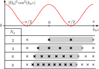
Figure 4: (Color online) Placement of atoms for periodic ensembles. At the top, the standing wave of the classical drive is plotted. In the table below, the crosses indicate the positions of the atoms in the standing wave of the classical drive for different values of the number of atoms per unit cell $N_{\text{u}}$. The thick crosses are the atoms in the chosen unit cell, and the thin crosses are the other atoms in the ensemble. The particular choice of the unit cell (gray) is such that the atoms with the non-zero classical drive are taken first (when propagating from the left), and the last atom is placed on the node of the classical drive (at $k_{0}z=\pi/2$) which effectively makes it a two-level atom.

For the regularly placed $\Lambda$-type atoms, we can also obtain dispersion relations, which are different from the predictions of the continuum model. To this end we consider the ensembles shown in Fig. 4. The atoms are spaced with a distance $d=\pi/(N_{\text{u}}k_{0})$, where we only take even $N_{\text{u}}$ for simplicity. (As explained above, adding integer multiples of $\pi/k_{0}$ to $d$ does not change the results.) A unit cell consists of $N_{\text{u}}-1$ atoms, which experience a non-zero classical drive, and one atom, which is placed such that the classical drive is zero, i.e. on the node of the standing wave of the classical drive. For such a setup, we show in App. F that the dispersion relation for two-photon detunings fulfilling

$$\delta\ll 2|\delta_{\text{S}}|\cos^{2}\mathinner{\left(\frac{\pi}{2}-\frac{\pi}{N_{\text{u}}}\right)}\approx 2|\delta_{\text{S}}|\mathinner{\left(\frac{\pi}{N_{\text{u}}}\right)}^{2}$$ (67)

(i.e. if frequency is within the smallest EIT window of the atoms that are not placed on the node) is given by

$$\delta\approx\frac{1}{2m}\mathinner{\left(\frac{q}{n_{0}}\right)}^{2},$$ (68)

where $n_{0}=1/d$, and

$$m=-\frac{(N_{\text{u}}-1)\Gamma_{\text{1D}}^{2}}{2N_{\text{u}}^{2}(\Delta_{\text{c}}+i\Gamma^{\prime}/2)|\Omega_{0}|^{2}}$$ (69)

is the effective mass. Note that the quadratic dispersion relation in Eq. (68) is of the same form as Eq. (32), but with the effective mass in Eq. (69) differing by a factor $2(N_{\text{u}}-1)/N_{\text{u}}^{2}$ from the one in Eq. (33).

Figure 5: (Color online) Log-log plot of the dispersion relations for $\Lambda$-type atoms with different placement of the atoms within the unit cell. The solid black (upper), red (lower) and blue (in between) curves are as in Fig. 2 and are shown for reference. The dashed green curves are for ensembles with regularly placed atoms (see Fig. 4) for the period lengths $N_{\text{u}}=2,4,8,16,32$. The dash-dotted magenta curves are for the same setups, but with a shifted standing wave of the classical drive: $\Omega(z)=\Omega_{0}\cos(k_{0}z+\varphi)$ with $\varphi=\pi/(2N_{\text{u}})$. The common parameters are: $\Gamma_{\text{1D}}/\Gamma=0.1$, $\Delta_{\text{c}}/\Gamma=-90$, $\Omega_{0}/\Gamma=1$. The density of the atoms $n_{0}$ is related to the spacing between the atoms $d$ by $n_{0}=1/d$. The distance $d$ depends on the desired period length and is given by $d=\pi/(N_{\text{u}}k_{0})$ (plus any integer multiple of $\pi/k_{0}$).

The above quadratic dispersion relation is obtained by placing the atoms such that one of them coincides exactly with the node of the standing wave of the classical drive. The dispersion relation can be completely changed, however, by shifting the position of the atoms relative to the drive. This can be achieved if the classical drive is given by $\Omega(z)=\Omega_{0}\cos(k_{0}z+\varphi)$ (with the situation above corresponding to $\varphi=0$). By choosing $\varphi=k_{0}d/2=\pi/(2N_{\text{u}})$, the node of the standing wave is placed exactly in the middle of the free-space separation between two atoms.

We show the numerically calculated dispersion relation for $\varphi=0$ and $\varphi=k_{0}d/2$ in Fig. 5. For $\varphi=0$ (dashed green curves), the dispersion relation becomes quadratic for small $\text{Re}[q]/n_{0}$ as given by Eq. (68). The range of validity of the quadratic approximation becomes smaller for increasing $N_{\text{u}}$, as predicted by the condition in Eq. (67). For $\varphi=k_{0}d/2$ (dash-dotted magenta curves), the dispersion relation becomes linear (parallel to the EIT dispersion relation) instead of quadratic for small $\text{Re}[q]/n_{0}$. As $N_{\text{u}}$ increases, both for $\varphi=0$ and $\varphi=k_{0}d/2$, the dispersion relation approaches the one for an ensemble of cold randomly placed $\Lambda$-type atoms (solid blue). The two choices of the phase, $\varphi=0$ and $\varphi=k_{0}d/2$, are thus similar to respectively the odd and even $n$ truncations in Fig. 2. In essence, having a finite number of atoms per unit cell gives a truncation because a finite number of atoms can only support a finite number of Fourier components of $\sigma_{ab}$ and $\sigma_{ac}$.

The two situations, $\varphi=0$ and $\varphi=k_{0}d/2$, considered in Fig. 5, represent the two extreme cases with the node of the classical drive either coinciding with an atom or being placed as far away from the atoms as possible. In between these extremes there is a whole continuum of possibilities. In general, if no atoms are placed at the nodes, all atoms will have a finite EIT window and hence the dispersion relation will be linear for sufficiently small $\delta$. This also implies that with a finite number of randomly placed stationary $\Lambda$-type atoms, it is impossible to realize a $\delta\propto|q|^{4/3}$ dispersion in the limit $\delta\rightarrow 0$, as there is formally zero probability for the point-like atoms to sit exactly at the nodes, and hence the dispersion relation will eventually cross over to the linear one.

V Scattering properties

A different way to compare the ensembles with regularly and randomly placed $\Lambda$-type atoms is to look at the scattering properties (transmission and reflection coefficients) of the whole ensemble. Contrary to the dispersion relation, which, in principle, is only valid for an infinite ensemble, the total number of atoms does matter for the scattering properties. If the number of the atoms is sufficiently large, the dispersion relation is still reflected in the behavior of the transmission and reflection coefficients. Hence, the scattering properties can also be used to characterize the dispersion relation. Below, the transmission coefficients $t$ and reflection coefficients $r$ will be obtained numerically by multiplying the transfer matrices for the atoms and free propagation to obtain the transfer matrix for the whole ensemble and afterwards extracting the scattering coefficients from this transfer matrix, as described in App. B. For regularly placed discrete atoms and the continuum model, one can derive closed-form expressions for the transfer matrix for the whole ensemble (see App. C).

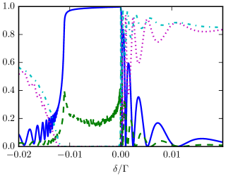
Figure 6: (Color online) Plot of transmittance $|t|^{2}$ and reflectance $|r|^{2}$ of ensembles with $N=4\cdot 10^{4}$ atoms. The dotted magenta and solid blue curves are respectively the transmittance and reflectance of an ensemble with regularly placed $\Lambda$-type atoms and $N_{\text{u}}=2$ (with the placement shown in Fig. 4). The dash-dotted cyan and dashed green curves are respectively the transmittance and reflectance of an ensemble with randomly placed $\Lambda$-type atoms and is averaged over 100 ensemble realizations. The other parameters are: $\Gamma_{\text{1D}}/\Gamma=0.1$, ${\Delta_{\text{c}}/\Gamma=-90}$, $\Omega_{0}/\Gamma=1$, $k_{0}/n_{0}=\pi/2$. The interval around $\delta=0$ is shown in more detail in Fig. 7(a).

Figure 7: (Color online) (a) Same as Fig. 6, but zoomed in around $\delta=0$. Additionally, the reflectance for an ensemble with randomly placed dual-V atoms is plotted (dashed red), and it completely overlaps the reflectance for the regularly placed $\Lambda$-type scheme. The dual-V scheme has the same parameters except that $\Omega_{0}$ is multiplied by $\sqrt{2}$ to make the dispersion relation equal to the one of the regularly placed $\Lambda$-type scheme. (b) Dispersion relations for $\Lambda$-type scheme: regularly placed (solid blue) and randomly placed (dashed green). The dispersion relation was calculated numerically with the transfer matrix formalism for the regularly placed ensemble, and using Eq. (56) for the randomly placed ensemble. The two horizontal dotted lines at ${\rm Re}[q]/n_{0}=\pi/N$ and ${\rm Re}[q]/n_{0}=2\pi/N$, give the condition for the first and the second high transmission resonance. At each intersection (for $\delta>0$) of these horizontal lines with the dispersion relation curves, vertical dotted lines are drawn, which can be seen to coincide with the high transmission resonances in (a).

In Figs. 6 and 7(a), we plot transmittance $|t|^{2}$ and reflectance $|r|^{2}$ for ensembles with regular ($N_{\text{u}}=2$) and random (average of 100 ensemble realizations) placement of $\Lambda$-type atoms. The latter case can also be calculated using the continuum model together with App. C. The main visible difference between the discrete model with random placement and the continuum model is that the former has noise in the region $-0.01\lesssim\delta/\Gamma\leq 0$ due to finite number of ensemble realizations. In Fig. 7(a) we additionally show the reflection coefficient for randomly placed dual-V atoms (single ensemble realization) with $\sigma_{+}$ input incident from the left and finding the left-moving $\sigma_{-}$ field to the left of the ensemble (such that the quadratic dispersion relation is valid). The reflection coefficient of the dual-V scheme overlaps completely with the reflection coefficient of the regularly placed $\Lambda$-type scheme, because we have increased the classical drive strength $\Omega_{0}$ of the dual-V scheme by a factor of $\sqrt{2}$ to make the masses in Eq. (33) and Eq. (69) equal.

The plots and the chosen parameters are similar to the ones in Ref. Hafezi et al. (2012). As opposed to Ref. Hafezi et al. (2012), however, we do not make the secular approximation for the $\Lambda$-type scheme, and this leads to very different results, which depend on how the atoms are placed (and whether we use the dual-V scheme instead). For the regularly placed $\Lambda$-type atoms, we see a clear signature of a photonic band gap in the region $-0.01\lesssim\delta/\Gamma\leq 0$, where there is a near unit reflectance and negligible transmittance. For the randomly placed $\Lambda$-type atoms, the situation is more complex with a similar negligible transmittance but a rather limited reflectance. For $\delta>0$, the position of the resonances with low reflection and high transmission corresponds to the condition $\sin\mathopen{}\mathinner{\left({\rm Re}[q]L\right)}=0$, i.e. there is a standing wave of the Bloch vectors inside the ensemble. Specifically, the high transmission resonance occurs each time ${\rm Re}[q]/n_{0}$ crosses a multiple of $\pi/N$, as can be seen in Fig. 7(b). This behavior can also be seen from the analytical results derived in App. C. Due to non-zero incoherent decay rate $\Gamma^{\prime}$, the sum $|t|^{2}+|r|^{2}$ is in general not equal to unity.

As we have shown above, the regularly and randomly placed $\Lambda$-type atoms have very different dispersion relations, and this translates into very different positions of the high transmission resonances in Figs. 6 and 7(a). For the randomly placed $\Lambda$-type scheme, there additionally occurs a high transmission resonance at $\delta=0$, since no atoms are placed exactly at the node of the standing wave of the classical drive, and hence all the atoms are transmissive due to EIT. For the regularly placed setup with $N_{\text{u}}=2$, half of the atoms are placed on the nodes and therefore behave as effective two-level atoms. For $\delta=0$, the other half of the atoms becomes transparent, and the whole ensemble is exactly equivalent to the atomic mirror Chang et al. (2012). For the dual-V atoms, as shown in App. E the reflection coefficients of a single atom do not become zero for $\delta=0$, regardless of how the individual atoms are placed.

VI Conclusion

We have analyzed a number of different setups for stationary light. These setups lead have different behaviors and dispersion relations depending on the exact details. For small Bloch vectors $q$, the dispersion relations are either linear, quadratic, or in between with $\delta\propto|q|^{4/3}$. For higher values of $q$, the dispersion relations either continue to have the same behavior, or the linear and quadratic dispersion relations may cross over into the $\delta\propto|q|^{4/3}$ results.

Overall, these results demonstrate the rich physics of stationary light. This opens the possibility of tailoring the light propagation to meet specific desired functionalities. In addition to the strong interest in understanding and controlling the propagation of light, another interesting possibility of stationary light is to use for non-linear optics. The ability to achieve a vanishing group velocity, and the corresponding increase in interaction time between photons in an optical pulse, may in principle lead to strong optical non-linearities down to the single photon level André and Lukin (2002); Chang et al. (2008); Hafezi et al. (2012). In order to fully assess such possibilities, it is essential to first have a thorough understanding of the linear properties of the system as determined in this work.

Appendix A Numerical methods for the continuum model

The truncations of both Eqs. (41) for the $\Lambda$-type scheme and Eqs. (59) for the dual-color scheme can be written

$$0=M\boldsymbol{\sigma}+g\sqrt{2\pi}V\boldsymbol{\mathcal{E}},$$ (70)

where

$$\boldsymbol{\sigma}=\begin{pmatrix}\vdots\\ \sigma_{ac}^{(+2)}\\ \sigma_{ab}^{(+1)}\\ \sigma_{ac}^{(0)}\\ \sigma_{ab}^{(-1)}\\ \sigma_{ac}^{(-2)}\\ \vdots\end{pmatrix},\quad V=\begin{pmatrix}\vdots&\vdots\\ 0&0\\ 1&0\\ 0&0\\ 0&1\\ 0&0\\ \vdots&\vdots\end{pmatrix},\quad\boldsymbol{\mathcal{E}}=\begin{pmatrix}\mathcal{E}_{+}\\ \mathcal{E}_{-}\end{pmatrix},$$ (71)

and the definition of the matrix $M$ depends on whether we consider Eqs. (41) or Eqs. (59). For Eqs. (41), we have

$$M=\begin{pmatrix}\ddots&\vdots&\vdots&\vdots&\vdots&\vdots&\scalebox{-1.0}[1.0]{$\ddots$}\\ \cdots&\delta&\Omega_{0}^{*}/2&0&0&0&\cdots\\ \cdots&\Omega_{0}/2&\tilde{\Delta}&\Omega_{0}/2&0&0&\cdots\\ \cdots&0&\Omega_{0}^{*}/2&\delta&\Omega_{0}^{*}/2&0&\cdots\\ \cdots&0&0&\Omega_{0}/2&\tilde{\Delta}&\Omega_{0}/2&\cdots\\ \cdots&0&0&0&\Omega_{0}^{*}/2&\delta&\cdots\\ \scalebox{-1.0}[1.0]{$\ddots$}&\vdots&\vdots&\vdots&\vdots&\vdots&\ddots\end{pmatrix}.$$ (72)

For Eqs. (59), we subtract $n\Delta_{\text{d}}$ ($n$ is the number of the row such that the middle one has $n=0$) from the diagonal elements of the above matrix.

We can write the equations for the electric field as

$$\begin{pmatrix}\frac{q}{n_{0}}&0\\ 0&-\frac{q}{n_{0}}\end{pmatrix}\boldsymbol{\mathcal{E}}=\frac{g\sqrt{2\pi}}{c}V^{\text{T}}\boldsymbol{\sigma},$$ (73)

where $V^{\text{T}}$ is the transpose of the matrix $V$. Using Eq. (70) and defining $M_{\mathcal{E}}=(\Gamma_{\text{1D}}/2)V^{\text{T}}M^{-1}V$, Eqs. (73) become

$$\begin{pmatrix}M_{\mathcal{E},11}+\frac{q}{n_{0}}&M_{\mathcal{E},12}\\ M_{\mathcal{E},21}&M_{\mathcal{E},22}-\frac{q}{n_{0}}\end{pmatrix}\boldsymbol{\mathcal{E}}=\begin{pmatrix}0\\ 0\end{pmatrix},$$ (74)

where $M_{\mathcal{E},kl}$ are the elements of $M_{\mathcal{E}}$. This equation is the equivalent of Eq. (45), but more general, since it is possible that $M_{\mathcal{E},11}\neq M_{\mathcal{E},22}$ (for the dual-color scheme). For Eq. (74) to have non-trivial solutions, the determinant of the matrix on the left hand side should be equal to zero. Hence, we get the equation

$$\mathinner{\left(\frac{q}{n_{0}}\right)}^{2}+\frac{q}{n_{0}}(M_{\mathcal{E},11}-M_{\mathcal{E},22})-\det(M_{\mathcal{E}})=0,$$ (75)

where $\det(M_{\mathcal{E}})$ is the determinant of $M_{\mathcal{E}}$. The dispersion relation is found by solving Eq. (75).

Appendix B Multi-mode transfer matrices

In this appendix, we show how to transform between scattering matrices and transfer matrices for the multi-mode electric fields. The approach is very similar to the transfer matrix theory used in elastostatics Stephen (2006). This is a more general version of the single-mode transfer matrix formalism Deutsch et al. (1995) that is commonly used for calculating electric fields in one-dimensional systems.

When one solves the scattering problem for an atom $j$ with position $z_{j}$, the result is the scattering matrix. In terms of the right-moving and left-moving parts of the electric field vector defined by Eq. (60) the relation is of the form

$$\begin{pmatrix}\mathbf{E}_{+}(z_{j}^{+})\\ \mathbf{E}_{-}(z_{j}^{-})\end{pmatrix}=\begin{pmatrix}S_{j,11}&S_{j,12}\\ S_{j,21}&S_{j,22}\end{pmatrix}\begin{pmatrix}\mathbf{E}_{+}(z_{j}^{-})\\ \mathbf{E}_{-}(z_{j}^{+})\end{pmatrix},$$ (76)

where the blocks $S_{j,kl}$ are in general $n_{\text{m}}$ by $n_{\text{m}}$ matrices describing the mixing of the $n_{\text{m}}$ possible modes propagating in each direction. The scattering matrix relates output fields on both sides of the scatterer to the inputs. We find the scattering matrices for the $\Lambda$-type and dual-V atoms in App. D and App. E respectively. In this appendix we only consider the general properties.

A transfer matrix for the atom

$$T_{\text{a},j}=\begin{pmatrix}T_{\text{a},j,{11}}&T_{\text{a},j,{12}}\\ T_{\text{a},j,{21}}&T_{\text{a},j,{22}}\end{pmatrix}$$ (77)

is a relation of the form

$$\begin{pmatrix}\mathbf{E}_{+}(z_{j}^{+})\\ \mathbf{E}_{-}(z_{j}^{+})\end{pmatrix}=T_{\text{a},j}\begin{pmatrix}\mathbf{E}_{+}(z_{j}^{-})\\ \mathbf{E}_{-}(z_{j}^{-})\end{pmatrix},$$ (78)

i.e. it relates the fields on one side of the atom to the fields on the other side. By rearranging Eq. (76) into the form of Eq. (78) one can show that

$$T_{\text{a},j,{11}}=S_{j,11}-S_{j,12}S_{j,22}^{-1}S_{j,21},$$ (79a)

$$T_{\text{a},j,{12}}=S_{j,12}S_{j,22}^{-1},$$ (79b)

$$T_{\text{a},j,{21}}=-S_{j,22}^{-1}S_{j,21},$$ (79c)

$$T_{\text{a},j,{22}}=S_{j,22}^{-1}.$$ (79d)

In App. D and App. E we show that the blocks of the scattering matrix for the $\Lambda$-type and dual-V atoms fulfill

$$S_{j,11}=S_{j,22}=S_{j,t},$$ (80a)

$$S_{j,12}=S_{j,21}=S_{j,r},$$ (80b)

where the matrices $S_{j,r}$ and $S_{j,t}$ are related by

$$S_{j,t}=I+S_{j,r},$$ (81)

with $I$ being the $n_{\text{m}}$ by $n_{\text{m}}$ identity matrix. From Eq. (81) we see that the matrices $S_{j,r}$ and $S_{j,t}$ commute. By writing

$$S_{j,r}S_{j,t}=S_{j,t}S_{j,r}$$ (82)

and multiplying both sides by $S_{j,t}^{-1}$ from right and left, we get

$$S_{j,t}^{-1}S_{j,r}=S_{j,r}S_{j,t}^{-1},$$ (83)

which implies that $S_{j,r}$ and $S_{j,t}^{-1}$ commute. This allows us to write Eqs. (79) in terms of a single matrix

$$\beta_{j}=-S_{j,t}^{-1}S_{j,r}.$$ (84)

We obtain

$$T_{\text{a},j,{11}}=S_{j,t}-S_{j,t}^{-1}S_{j,r}^{2}=I-\beta_{j},$$ (85a)

$$T_{\text{a},j,{12}}=S_{j,t}^{-1}S_{j,r}=-\beta_{j},$$ (85b)

$$T_{\text{a},j,{21}}=-S_{j,t}^{-1}S_{j,r}=\beta_{j},$$ (85c)

$$T_{\text{a},j,{22}}=S_{j,t}^{-1}=I+\beta_{j}.$$ (85d)

For the $\Lambda$-type atoms and dual-V atoms with ${\Omega_{+}=\Omega_{-}}$ and $\omega_{b_{+}c}=\omega_{b_{-}c}$, $\beta_{j}$ is symmetric, i.e. $\beta_{j}=\beta_{j}^{\text{T}}$, where $\beta_{j}^{\text{T}}$ is the transpose of $\beta_{j}$ (see App. D and App. E). Using this fact we also see that the transfer matrix $T_{\text{a},j}$ is symplectic. This means that if we define a matrix

$$J=\begin{pmatrix}0&I\\ -I&0\end{pmatrix},$$ (86)

where zeros mean $n_{\text{m}}$ by $n_{\text{m}}$ matrices with all elements equal to zero, then it holds that

$$T_{\text{a},j}^{\text{T}}JT_{\text{a},j}=J.$$ (87)

This can be seen from the fact that if $\beta_{j}$ is symmetric, then so is $I\pm\beta_{j}$, and Eq. (87) can be shown by writing out the left hand side using Eqs. (85).

Free propagation of the electric field with the wave vector $k_{0}$ for a distance $d$ has the transfer matrix

$$T_{\text{f}}=\begin{pmatrix}e^{ik_{0}d}I&0\\ 0&e^{-ik_{0}d}I\end{pmatrix}.$$ (88)

The free propagation matrix $T_{\text{f},j}$ between atoms $j$ and $j+1$ at positions $z_{j}$ and $z_{j+1}$ fulfills $\mathbf{E}(z_{j+1}^{-})=T_{\text{f},j}\mathbf{E}(z_{j}^{+})$ and is given by Eq. (88) with $d=z_{j+1}-z_{j}$.

The free propagation transfer matrices $T_{\text{f},j}$ are always symplectic. Therefore, the transfer matrix of a unit cell (or the whole ensemble), which is a product of the matrices $T_{\text{a},j}$ and $T_{\text{f},j}$, is symplectic if $T_{\text{a},j}$ is symplectic for all $j$. This can be seen by considering a product of two symplectic transfer matrices, $T_{1}$ and $T_{2}$. It holds that

$$(T_{1}T_{2})^{\text{T}}J(T_{1}T_{2})=T_{2}^{\text{T}}T_{1}^{\text{T}}JT_{1}T_{2}=T_{2}^{\text{T}}JT_{2}=J,$$ (89)

hence the matrix $T_{1}T_{2}$ is symplectic.

For the purposes of finding the dispersion relation, we need to diagonalize the transfer matrix for the unit cell $T_{\text{cell}}$. Assuming that the unit cell has length $L_{\text{u}}$ and starts at $z=0$, we have the relation

$$\begin{pmatrix}\mathbf{E}_{+}(L_{\text{u}}^{+})\\ \mathbf{E}_{-}(L_{\text{u}}^{+})\end{pmatrix}=T_{\text{cell}}\begin{pmatrix}\mathbf{E}_{+}(0^{-})\\ \mathbf{E}_{-}(0^{-})\end{pmatrix}.$$ (90)

We note that if $T_{\text{cell}}$ is symplectic, then it has the property that its eigenvalues occur in reciprocal pairs. To see this, assume that $\mathbf{E}_{\lambda}$ is an eigenvector of $T_{\text{cell}}$ with eigenvalue $\lambda$, i.e.

$$T_{\text{cell}}\mathbf{E}_{\lambda}=\lambda\mathbf{E}_{\lambda}.$$ (91)

Then using the property $T_{\text{cell}}^{\text{T}}JT_{\text{cell}}=J$ we have

$$T_{\text{cell}}^{\text{T}}(J\mathbf{E}_{\lambda})=T_{\text{cell}}^{\text{T}}JT_{\text{cell}}(1/\lambda)\mathbf{E}_{\lambda}=(1/\lambda)(J\mathbf{E}_{\lambda}).$$ (92)

Therefore, $J\mathbf{E}_{\lambda}$ is an eigenvector of $T_{\text{cell}}^{\text{T}}$ with the eigenvalue $1/\lambda$. Since $T_{\text{cell}}$ and $T_{\text{cell}}^{\text{T}}$ have the same set of eigenvalues, $1/\lambda$ is also an eigenvalue of $T_{\text{cell}}$.

The transmission and reflection coefficients for the whole ensemble can be obtained from its transfer matrix $T_{\text{e}}$. Assuming that the ensemble has length $L$ and starts at $z=0$, we have the relation

$$\begin{pmatrix}\mathbf{E}_{+}(L^{+})\\ \mathbf{E}_{-}(L^{+})\end{pmatrix}=\begin{pmatrix}T_{\text{e},{11}}&T_{\text{e},{12}}\\ T_{\text{e},{21}}&T_{\text{e},{22}}\end{pmatrix}\begin{pmatrix}\mathbf{E}_{+}(0^{-})\\ \mathbf{E}_{-}(0^{-})\end{pmatrix}.$$ (93)

For concreteness, we assume a two-mode transfer matrix as is relevant for the dual-V scheme. Hence, the vectors $\mathbf{E}_{\pm}$ have two elements. We adopt the convention that the first element is a $\sigma_{+}$ component, and the second element is the $\sigma_{-}$ component of the field (the same definition as in Eq. (62)). As an example, consider a scattering problem with the incoming fields

$$\mathbf{E}_{+}(0^{-})=\begin{pmatrix}1\\ 0\end{pmatrix},\quad\mathbf{E}_{-}(L^{+})=\begin{pmatrix}0\\ 0\end{pmatrix},$$ (94)

i.e. there is only a $\sigma_{+}$ input field from the left. We want to find the outgoing fields: $\mathbf{E}_{+}(L^{+})$ (the transmitted field) and $\mathbf{E}_{-}(0^{-})$ (the reflected field).

After insertion of Eqs. (94) into Eq. (93) we find

$$\mathbf{E}_{-}(0^{-})=-T_{\text{e},{22}}^{-1}T_{\text{e},{12}}\mathbf{E}_{+}(0^{-}),$$ (95a)

$$\mathbf{E}_{+}(L^{+})=(T_{\text{e},{11}}-T_{\text{e},{12}}T_{\text{e},{22}}^{-1}T_{\text{e},{21}})\mathbf{E}_{+}(0^{-}).$$ (95b)

For the single-mode transfer matrices, $T_{\text{e},{kl}}$ are scalars. Furthermore, from Eqs. (85) and (88) we see that the transfer matrices for atoms and free propagation have determinants equal to unity. Using the fact that $\det(T_{1}T_{2})=\det(T_{1})\det(T_{2})$ for any two square matrices $T_{1}$ and $T_{2}$, we have $T_{\text{e},{11}}T_{\text{e},{22}}-T_{\text{e},{12}}T_{\text{e},{21}}=\det(T_{\text{e}})=1$. This leads to a simplification of Eqs. (95), so that they become

$$E_{-}(0^{-})=-(T_{\text{e},{12}}/T_{\text{e},{22}})E_{+}(0^{-}),$$ (96a)

$$E_{+}(L^{+})=(1/T_{\text{e},{22}})E_{+}(0^{-}).$$ (96b)

Appendix C Transfer matrix for a uniform ensemble

In this appendix, we will find closed-form expressions for the transfer matrix for the whole ensemble that either consists of $n_{\text{e}}$ copies of the same unit cell with the transfer matrix

$$T_{\text{cell}}=\begin{pmatrix}T_{11}&T_{12}\\ T_{21}&T_{22}\end{pmatrix}$$ (97)

in the discrete case, or is governed by the equations of the form

$$\mathinner{\dfrac{\partial{}}{\partial{z}}}\begin{pmatrix}\mathcal{E}_{+}\\ \mathcal{E}_{-}\end{pmatrix}=in_{0}\begin{pmatrix}-\alpha_{1}&-\alpha_{2}\\ \alpha_{2}&\alpha_{1}\end{pmatrix}\begin{pmatrix}\mathcal{E}_{+}\\ \mathcal{E}_{-}\end{pmatrix}$$ (98)

in the continuum case. For the continuum case, we note that Eqs. (22a) for the dual-V scheme and the equivalent equations for the $\Lambda$-type scheme can be written in the form above (neglecting the vacuum dispersion relation) with $\alpha_{1}$ and $\alpha_{2}$ being given by either Eqs. (30) or Eqs. (55), depending on the scheme.

The starting point of the derivation is diagonalizing either the transfer matrix in Eq. (97) or the matrix in Eq. (98). This gives

$$\begin{pmatrix}T_{11}&T_{12}\\ T_{21}&T_{22}\end{pmatrix}=V_{\text{cell}}D_{\text{cell}}V_{\text{cell}}^{-1},$$ (99)

$$\begin{pmatrix}-\alpha_{1}&-\alpha_{2}\\ \alpha_{2}&\alpha_{1}\end{pmatrix}=V_{\alpha}D_{\alpha}V_{\alpha}^{-1},$$ (100)

where the diagonal matrix $D_{\text{cell}}$ has elements (eigenvalues) $\exp(\pm i\tilde{q}L_{\text{u}})$, and the diagonal matrix $D_{\alpha}$ has elements $\pm q/n_{0}$. Here we use the relation (63) between the Bloch vector and the elements of $D_{\text{cell}}$ for brevity. The eigenvector matrices are

$$V_{\text{cell}}=\begin{pmatrix}1&1\\ (e^{i\tilde{q}L_{\text{u}}}-T_{11})/T_{12}&(e^{-i\tilde{q}L_{\text{u}}}-T_{11})/T_{12}\end{pmatrix},$$ (101)

$$V_{\alpha}=\begin{pmatrix}1&1\\ -(q/n_{0}+\alpha_{1})/\alpha_{2}&-(-q/n_{0}+\alpha_{1})/\alpha_{2}\end{pmatrix}.$$ (102)

In the discrete case, the transfer matrix for the whole ensemble is $T_{\text{e}}=T_{\text{cell}}^{n_{\text{e}}}$, where $n_{\text{e}}=L/L_{\text{u}}$ is an integer. This expression can be written as

$$\begin{aligned} T_{\text{e}}&=V_{\text{cell}}D_{\text{cell}}^{n_{\text{e}}}V_{\text{cell}}^{-1}\\ &=V_{\text{cell}}\mathinner{\left(\cos(\tilde{q}L)I+i\sin(\tilde{q}L)\sigma_{z}\right)}V_{\text{cell}}^{-1}\\ &=\cos(\tilde{q}L)I+i\sin(\tilde{q}L)V_{\text{cell}}\sigma_{z}V_{\text{cell}}^{-1},\end{aligned}$$ (103)

where $I$ is the identity matrix and

$$\sigma_{z}=\begin{pmatrix}1&0\\ 0&-1\end{pmatrix}.$$ (104)

By doing the matrix multiplications and using $2\cos(\tilde{q}L_{\text{u}})=\text{tr}(T_{\text{cell}})=T_{11}+T_{12}$ and $\det(T_{\text{cell}})=1$, we find

$$V_{\text{cell}}\sigma_{z}V_{\text{cell}}^{-1}=\frac{1}{\sin(\tilde{q}L_{\text{u}})}\begin{pmatrix}\frac{i}{2}(T_{22}-T_{11})&-iT_{12}\\ -iT_{21}&-\frac{i}{2}(T_{22}-T_{11})\end{pmatrix}.$$ (105)

In the continuum case, the transfer matrix for the whole ensemble is

$$\begin{aligned} T_{\text{e}}&=\exp\mathinner{\left(in_{0}\begin{pmatrix}-\alpha_{1}&-\alpha_{2}\\ \alpha_{2}&\alpha_{1}\end{pmatrix}L\right)}\\ &=\cos(qL)I+i\sin(qL)V_{\alpha}\sigma_{z}V_{\alpha}^{-1},\end{aligned}$$ (106)

where (using $\alpha_{1}^{2}-(q/n_{0})^{2}-\alpha_{2}^{2}=0$)

$$V_{\alpha}\sigma_{z}V_{\alpha}^{-1}=\frac{1}{q/n_{0}}\begin{pmatrix}-\alpha_{1}&-\alpha_{2}\\ \alpha_{2}&\alpha_{1}\end{pmatrix}.$$ (107)

Appendix D Scattering matrix for $\Lambda$-type atoms

In this appendix, we find the scattering matrix (i.e. the reflection and transmission coefficients) for a $\Lambda$-type atom (see Fig. 1(b)). The derivation is based on Ref. Chang et al. (2011). The electric field is given by the operator

$$\hat{\mathcal{E}}(z)=\hat{\mathcal{E}}_{+}(z)e^{ik_{0}(z-z_{j})}+\hat{\mathcal{E}}_{-}(z)e^{-ik_{0}(z-z_{j})}.$$ (108)

Compared to the continuum model, we have shifted the spatial phases such that they vanish at the position of the atom $z_{j}$ ($j$ is the index of the atom). The effects of the propagation phases will be accounted for separately by the transfer matrices of free propagation.

The Hamiltonian (34), which we have used for the continuum model, can also be used to describe a single $\Lambda$-type atom, since the discrete nature of the atoms is still present due to the definition of the atomic operators given by Eq. (9). Because of considering only a single atom, Eq. (9) becomes $\hat{\sigma}_{\alpha\beta}(z)=\frac{1}{n_{0}}\delta(z-z_{j})\hat{\sigma}_{\alpha\beta,j}$, and inserting this into Eqs. (34) results in

$$\begin{aligned} \hat{H}_{\text{3,a}}=-\hbar\mathinner{\left[\tilde{\Delta}_{0}\hat{\sigma}_{bb,j}+\delta_{0}\hat{\sigma}_{cc,j}\right]},\end{aligned}$$ (109a)

$$\begin{aligned} \hat{H}_{\text{3,i}}=&-\hbar\mathinner{\left[\hat{\sigma}_{bc,j}\Omega(z_{j})+\text{H.c.}\right]}\\ &-\hbar g\sqrt{2\pi}\left[\hat{\sigma}_{ba,j}\hat{\mathcal{E}}(z_{j})+\text{H.c.}\right],\end{aligned}$$ (109b)

$$\begin{aligned} \hat{H}_{\text{3,p}}=-i\hbar c\int\mathinner{\left[\hat{\mathcal{E}}_{+}^{\dagger}(z)\mathinner{\dfrac{\partial{}\hat{\mathcal{E}}_{+}(z)}{\partial{z}}}-\hat{\mathcal{E}}_{-}^{\dagger}(z)\mathinner{\dfrac{\partial{}\hat{\mathcal{E}}_{-}(z)}{\partial{z}}}\right]}\operatorname{d\!}z.\end{aligned}$$ (109c)

From the Hamiltonian, we get the Heisenberg equations for the atom

$$\mathinner{\dfrac{\partial{}\sigma_{ab,j}}{\partial{t}}}=i\tilde{\Delta}_{0}\sigma_{ab,j}+i\Omega(z_{j})\sigma_{ac,j}+ig\sqrt{2\pi}\mathcal{E}(z_{j},t),$$ (110a)

$$\mathinner{\dfrac{\partial{}\sigma_{ac,j}}{\partial{t}}}=i\delta_{0}\sigma_{ac,j}+i\Omega^{*}(z_{j})\sigma_{ab,j}.$$ (110b)

These equations are similar to Eqs. (36), except that here we do not make the continuum approximation.

For the electric field we have the equations

$$\mathinner{\left(\mathinner{\dfrac{\partial{}}{\partial{t}}}\pm c\mathinner{\dfrac{\partial{}}{\partial{z}}}\right)}\mathcal{E}_{\pm}(z,t)=ig\sqrt{2\pi}\delta(z-z_{j})\sigma_{ab,j},$$ (111)

which are exactly the same as Eqs. (35) due the definition (9). In this form, however, we can formally solve them Chang et al. (2012), so that we obtain

$$\begin{aligned} \mathcal{E}_{\pm}(z,t)=\;&\mathcal{E}_{\pm,\text{in}}(z\mp ct)\\ &+\frac{ig\sqrt{2\pi}}{c}\theta\mathopen{}\mathinner{\left(\pm(z-z_{j})\right)}\sigma_{ab,j}\mathopen{}\mathinner{\left(t\mp\frac{z-z_{j}}{c}\right)},\end{aligned}$$ (112)

where $\mathcal{E}_{\pm,\text{in}}(z\pm ct)$ are the input fields, and $\theta$ is the Heaviside theta function.

Since the scattering problem is symmetric, and since the equations are linear, we can gain full information about the scattering by setting $\mathcal{E}_{+,\text{in}}(z-ct)=1$ and $\mathcal{E}_{-,\text{in}}(z+ct)=0$ in Eqs. (112). Then we find the total electric field (108) to be

$$\mathcal{E}(z_{j},t)=1+\frac{ig\sqrt{2\pi}}{c}\sigma_{ab,j}\mathinner{\left(t\right)}$$ (113)

Upon inserting this expression into (110a), we obtain

$$\mathinner{\dfrac{\partial{}\sigma_{ab,j}}{\partial{t}}}=i\mathinner{\left(\tilde{\Delta}_{0}+i\frac{\Gamma_{\text{1D}}}{2}\right)}\sigma_{ab,j}+i\Omega(z_{j})\sigma_{ac,j}+ig\sqrt{2\pi}.$$ (114)

After Fourier transforming Eqs. (112) we get the reflection and transmission coefficients

$$r_{j}=\mathcal{E}_{-}(z_{j}^{-},\omega)=\frac{ig\sqrt{2\pi}}{c}\sigma_{ab,j}(\omega),$$ (115a)

$$t_{j}=\mathcal{E}_{+}(z_{j}^{+},\omega)=1+r_{j}.$$ (115b)

We also Fourier transform Eq. (110b) and Eq. (114) and get

$$0=i\mathinner{\left(\tilde{\Delta}+i\frac{\Gamma_{\text{1D}}}{2}\right)}\sigma_{ab,j}+i\Omega(z_{j})\sigma_{ac,j}+ig\sqrt{2\pi},$$ (116a)

$$0=i\delta\sigma_{ac,j}+i\Omega^{*}(z_{j})\sigma_{ab,j},$$ (116b)

where, as before, we have absorbed the Fourier frequency variable $\omega$ into the detunings by defining $\tilde{\Delta}=\tilde{\Delta}_{0}+\omega$ and $\delta=\delta_{0}+\omega$.

Now we solve Eqs. (115) and (116) and find

$$r_{j}=-\frac{i(\Gamma_{\text{1D}}/2)\delta}{(\tilde{\Delta}+i\Gamma_{\text{1D}}/2)\delta-|\Omega(z_{j})|^{2}},$$ (117a)

$$t_{j}=\frac{\tilde{\Delta}\delta-|\Omega(z_{j})|^{2}}{(\tilde{\Delta}+i\Gamma_{\text{1D}}/2)\delta-|\Omega(z_{j})|^{2}}.$$ (117b)

The parameter (84), in terms of which the blocks of the transfer matrix (85) are written, is a scalar in the single-mode case and is given by

$$\beta_{j}=-\frac{r_{j}}{t_{j}}=\frac{i(\Gamma_{\text{1D}}/2)\delta}{\tilde{\Delta}\delta-|\Omega(z_{j})|^{2}}.$$ (118)

Appendix E Scattering matrix for the dual-V atoms.

The derivation of the scattering matrix for the dual-V atoms proceeds in a similar manner as the derivation for the $\Lambda$-type atoms in App. D. Similar to Eq. (108) we define the electric field operators

$$\hat{\mathcal{E}}_{\sigma_{\pm}}(z)=\hat{\mathcal{E}}_{\sigma_{\pm},+}(z)e^{ik_{0}(z-z_{j})}+\hat{\mathcal{E}}_{\sigma_{\pm},-}(z)e^{-ik_{0}(z-z_{j})}.$$ (119)

The Hamiltonian for a single dual-V atom interacting with light is given by Eqs. (13) with the atomic operators $\hat{\sigma}_{\alpha\beta}(z)=\frac{1}{n_{0}}\delta(z-z_{j})\hat{\sigma}_{\alpha\beta,j}$ (special case of the definition (9)). Therefore, Eqs. (13) can be written

$$\begin{aligned} \hat{H}_{\text{V,a}}=-\hbar\mathinner{\left[\sum_{\alpha\in\{+,-\}}\tilde{\Delta}_{0}^{(\alpha)}\hat{\sigma}_{b_{\alpha}b_{\alpha},j}+\delta_{0}\hat{\sigma}_{cc,j}\right]},\end{aligned}$$ (120a)

$$\begin{aligned} \hat{H}_{\text{V,i}}=&-\hbar\sum_{\alpha\in\{+,-\}}\Bigg{\{}\mathinner{\left[\hat{\sigma}_{b_{\alpha}c,j}\Omega_{\alpha}e^{\alpha ik_{\text{c}}z_{j}}+\text{H.c.}\right]}\\ &+g\sqrt{2\pi}\left[\hat{\sigma}_{b_{\alpha}a,j}\hat{\mathcal{E}}_{\sigma_{\alpha}}(z_{j})+\text{H.c.}\right]\Bigg{\}},\end{aligned}$$ (120b)

$$\begin{aligned} \hat{H}_{\text{V,p}}=-i\hbar c\int\sum_{\alpha\in\{+,-\}}\Bigg{[}&\hat{\mathcal{E}}_{\sigma_{\alpha},+}^{\dagger}(z)\mathinner{\dfrac{\partial{}\hat{\mathcal{E}}_{\sigma_{\alpha},+}(z)}{\partial{z}}}\\ &-\hat{\mathcal{E}}_{\sigma_{\alpha},-}^{\dagger}(z)\mathinner{\dfrac{\partial{}\hat{\mathcal{E}}_{\sigma_{\alpha},-}(z)}{\partial{z}}}\Bigg{]}\operatorname{d\!}z.\end{aligned}$$ (120c)

From the Hamiltonian, the equations for the atom are

$$\begin{aligned} \mathinner{\dfrac{\partial{}\sigma_{ab_{\pm},j}}{\partial{t}}}=\;&i\tilde{\Delta}_{0}^{(\pm)}\sigma_{ab_{\pm},j}+i\Omega_{\pm}\sigma_{ac,j}e^{\pm ik_{\text{c}}z_{j}}\\ &+ig\sqrt{2\pi}\mathcal{E}_{\sigma_{\pm}}(z_{j},t),\end{aligned}$$ (121a)

$$\mathinner{\dfrac{\partial{}\sigma_{ac,j}}{\partial{t}}}=i\delta_{0}\sigma_{ac,j}+i\Omega_{+}^{*}\sigma_{ab_{+},j}e^{-ik_{\text{c}}z_{j}}+i\Omega_{-}^{*}\sigma_{ab_{-},j}e^{ik_{\text{c}}z_{j}}.$$ (121b)

The formal solutions to the equations for the field are

$$\begin{aligned} &\mathcal{E}_{\sigma_{+},\pm}(z,t)=\mathcal{E}_{\sigma_{+},\pm,\text{in}}(z\mp ct)\\ &+\frac{ig\sqrt{2\pi}}{c}\theta\mathopen{}\mathinner{\left(\pm(z-z_{j})\right)}\sigma_{ab_{+},j}\mathopen{}\mathinner{\left(t\mp\frac{z-z_{j}}{c}\right)},\end{aligned}$$ (122a)

$$\begin{aligned} &\mathcal{E}_{\sigma_{-},\pm}(z,t)=\mathcal{E}_{\sigma_{-},\pm,\text{in}}(z\mp ct)\\ &+\frac{ig\sqrt{2\pi}}{c}\theta\mathopen{}\mathinner{\left(\pm(z-z_{j})\right)}\sigma_{ab_{-},j}\mathopen{}\mathinner{\left(t\mp\frac{z-z_{j}}{c}\right)}.\end{aligned}$$ (122b)

Because of the symmetry of the system, we only need to consider two cases: $\mathcal{E}_{\sigma_{+},+,\text{in}}(z_{j}-ct)=1$ with the rest of the input fields being zero, and $\mathcal{E}_{\sigma_{-},+,\text{in}}(z_{j}-ct)=1$ with the rest of the input fields being zero.

Starting with the first case ($\mathcal{E}_{\sigma_{+},+,\text{in}}(z_{j}-ct)=1$) and Fourier transforming, Eqs. (121) become

$$0=i\tilde{\Delta}^{(+)}_{\text{tot}}\sigma_{ab_{+},j}+i\Omega_{+}\sigma_{ac,j}e^{ik_{\text{c}}z_{j}}+ig\sqrt{2\pi},$$ (123a)

$$0=i\tilde{\Delta}^{(-)}_{\text{tot}}\sigma_{ab_{-},j}+i\Omega_{-}\sigma_{ac,j}e^{-ik_{\text{c}}z_{j}},$$ (123b)

$$0=i\delta\sigma_{ac,j}+i\Omega_{+}^{*}\sigma_{ab_{+},j}e^{-ik_{\text{c}}z_{j}}+i\Omega_{-}^{*}\sigma_{ab_{-},j}e^{ik_{\text{c}}z_{j}},$$ (123c)

with $\tilde{\Delta}^{(\pm)}_{\text{tot}}=\tilde{\Delta}_{0}^{(\pm)}+i(\Gamma_{\text{1D}}/2)+\omega$ defined for notational convenience, such that we have now absorbed the total decay rate $\Gamma=\Gamma^{\prime}+\Gamma_{\text{1D}}$ into $\tilde{\Delta}^{(\pm)}_{\text{tot}}$; and $\delta=\delta_{0}+\omega$. From Eqs. (122) we have the relations

$$r_{j,++}=\mathcal{E}_{\sigma_{+},-}(z_{j}^{-},\omega)=\frac{ig\sqrt{2\pi}}{c}\sigma_{ab_{+},j}(\omega),$$ (124a)

$$t_{j,++}=\mathcal{E}_{\sigma_{+},+}(z_{j}^{+},\omega)=1+r_{j,++},$$ (124b)

$$r_{j,+-}=\mathcal{E}_{\sigma_{-},-}(z_{j}^{-},\omega)=\frac{ig\sqrt{2\pi}}{c}\sigma_{ab_{-},j}(\omega),$$ (124c)

$$t_{j,+-}=\mathcal{E}_{\sigma_{-},+}(z_{j}^{+},\omega)=r_{j,+-}.$$ (124d)

After solving Eqs. (123) and (124) (with $k_{\text{c}}\approx k_{0}$) we get

$$r_{j,++}=-\frac{i(\Gamma_{\text{1D}}/2)\mathinner{\left(\tilde{\Delta}^{(-)}_{\text{tot}}\delta-|\Omega_{-}|^{2}\right)}}{\tilde{\Delta}^{(+)}_{\text{tot}}\tilde{\Delta}^{(-)}_{\text{tot}}\delta-\tilde{\Delta}^{(+)}_{\text{tot}}|\Omega_{-}|^{2}-\tilde{\Delta}^{(-)}_{\text{tot}}|\Omega_{+}|^{2}},$$ (125a)

$$t_{j,++}=1+r_{j,++},$$ (125b)

$$r_{j,+-}=t_{j,+-}=\frac{\Omega_{-}\Omega_{+}^{*}e^{-2ik_{0}z_{j}}}{\tilde{\Delta}^{(-)}_{\text{tot}}\delta-|\Omega_{-}|^{2}}r_{j,++}.$$ (125c)

For the second case ($\mathcal{E}_{\sigma_{-},+,\text{in}}(z_{j}-ct)=1$), instead of Eqs. (123) we have

$$0=i\tilde{\Delta}^{(+)}_{\text{tot}}\sigma_{ab_{+},j}+i\Omega_{+}\sigma_{ac,j}e^{ik_{\text{c}}z_{j}},$$ (126a)

$$0=i\tilde{\Delta}^{(-)}_{\text{tot}}\sigma_{ab_{-},j}+i\Omega_{-}\sigma_{ac,j}e^{-ik_{\text{c}}z_{j}}+ig\sqrt{2\pi},$$ (126b)

$$0=i\delta\sigma_{ac,j}+i\Omega_{+}^{*}\sigma_{ab_{+},j}e^{-ik_{\text{c}}z_{j}}+i\Omega_{-}^{*}\sigma_{ab_{-},j}e^{ik_{\text{c}}z_{j}}.$$ (126c)

Instead of Eqs. (125) we have

$$r_{j,--}=\mathcal{E}_{\sigma_{-},-}(z_{j}^{-},\omega)=\frac{ig\sqrt{2\pi}}{c}\sigma_{ab_{-},j}(\omega),$$ (127a)

$$t_{j,--}=\mathcal{E}_{\sigma_{-},+}(z_{j}^{+},\omega)=1+r_{j,--},$$ (127b)

$$r_{j,-+}=\mathcal{E}_{\sigma_{+},-}(z_{j}^{-},\omega)=\frac{ig\sqrt{2\pi}}{c}\sigma_{ab_{+},j}(\omega),$$ (127c)

$$t_{j,-+}=\mathcal{E}_{\sigma_{+},+}(z_{j}^{+},\omega)=r_{j,-+}.$$ (127d)

After solving Eqs. (126) and (127) we get

$$r_{j,--}=-\frac{i(\Gamma_{\text{1D}}/2)\mathinner{\left(\tilde{\Delta}^{(+)}_{\text{tot}}\delta-|\Omega_{+}|^{2}\right)}}{\tilde{\Delta}^{(+)}_{\text{tot}}\tilde{\Delta}^{(-)}_{\text{tot}}\delta-\tilde{\Delta}^{(+)}_{\text{tot}}|\Omega_{-}|^{2}-\tilde{\Delta}^{(-)}_{\text{tot}}|\Omega_{+}|^{2}},$$ (128a)

$$t_{j,--}=1+r_{j,--},$$ (128b)

$$r_{j,-+}=t_{j,-+}=\frac{\Omega_{+}\Omega_{-}^{*}e^{2ik_{0}z_{j}}}{\tilde{\Delta}^{(+)}_{\text{tot}}\delta-|\Omega_{+}|^{2}}r_{j,--}.$$ (128c)

In terms of Eqs. (125) and (128), the blocks of the scattering matrix in Eq. (76) with the definition of the fields in Eq. (62) are

$$S_{j,11}=S_{j,22}=\begin{pmatrix}t_{j,++}&t_{j,-+}\\ t_{j,+-}&t_{j,--}\end{pmatrix},$$ (129a)

$$S_{j,12}=S_{j,21}=\begin{pmatrix}r_{j,++}&r_{j,-+}\\ r_{j,+-}&r_{j,--}\end{pmatrix}.$$ (129b)

If we use the definitions of Eq. (80), we further see that Eq. (81) holds.

As for the calculations using the continuum model in Sec. III.1, we will also use ${\omega_{b_{+}c}=\omega_{b_{-}c}}$ and ${\Omega_{+}=\Omega_{-}=\Omega_{0}/2}$ in the discrete model. This implies that $r_{j,+-}=r_{j,-+}$, and hence that the matrices $S_{j,kl}$ are symmetric. Since the product of commuting symmetric matrices is symmetric, it also follows that $\beta_{j}$ given by Eq. (84) is symmetric.

Appendix F Effective mass for the regularly placed $\Lambda$-type scheme

In this appendix, we derive the expression for the effective mass (69). For the single-mode case, we have that

$$\text{tr}(T_{\text{cell}})=\lambda+1/\lambda,$$ (130)

where $\text{tr}(T_{\text{cell}})$ is the trace of $T_{\text{cell}}$, and $\lambda$ is one of the eigenvalues of $T_{\text{cell}}$. Since the length of the unit cell is $L_{\text{u}}=\pi/k_{0}$, Eq. (130) together with Eq. (64) implies that

$$\cos(qL_{\text{u}})=-\frac{1}{2}\text{tr}(T_{\text{cell}}),$$ (131)

The right hand side of this equation is a function of $\delta$. We will solve it perturbatively to find $\delta$ as a function of $q$. Then the mass is found as the coefficient of the second order term in $q$ in the series expansion.

For small $\delta$ and $\Omega_{0}\neq 0$, the scattering coefficient $\beta_{j}$ (given by Eq. (118) with $\Omega(z_{j})=\Omega_{0}\cos(k_{0}z_{j})$) can be approximated by

$$\beta_{j}\approx-i\frac{\Gamma_{\text{1D}}}{2|\Omega_{0}|^{2}\cos^{2}(k_{0}z_{j})}\delta.$$ (132)

The precise condition for this approximation to be valid is that

$$\delta\ll\frac{|\Omega_{0}|^{2}}{|\tilde{\Delta}|}\cos^{2}(k_{0}z_{j})$$ (133)

has to be fulfilled for all the atoms in the unit cell which experience non-vanishing classical drive, i.e. the frequency has to be within their EIT windows. The right hand side of Eq. (133) is smallest for the atoms placed at $k_{0}z_{j}=\pm(\pi/2-\pi/N_{\text{u}})$ (see Fig. 4). This leads to the condition given by Eq. (67) of the main text.

For the chosen unit cells in Fig. 4 and numbering the atoms from the left (such that the leftmost atom in the unit cell has index $j=1$), we have within the approximation above that $\beta_{j}$ for ${1\leq j\leq N_{\text{u}}-1}$ is inversely proportional to the classical field strength. We define

$$\beta_{\text{c}}=-i\frac{\Gamma_{\text{1D}}}{2|\Omega_{0}|^{2}}\delta,$$ (134)

so that for the chosen unit cells we have

$$\beta_{j}\approx\frac{\beta_{\text{c}}}{\cos^{2}((j-N_{\text{u}}/2)k_{0}d)}$$ (135)

with $d=\pi/(N_{\text{u}}k_{0})$.

On the other hand, the last atom in the unit cell, which is positioned at the node of the standing wave of the classical drive, will instead be described by Eq. (118) with ${\Omega(z_{j})=0}$, i.e.

$$\beta_{N_{\text{u}}}\approx\frac{\Gamma_{\text{1D}}}{\Gamma^{\prime}-2i\Delta_{\text{c}}},$$ (136)

where we have approximated $\Delta\approx\Delta_{\text{c}}$, since we assume $\delta\ll\Delta_{\text{c}}$. This last atom effectively behaves as a two-level atom.

The claim now is that in this approximation and for even $N_{\text{u}}$, we have to first order in $\beta_{\text{c}}$ that

$$\frac{1}{2}\text{tr}(T_{\text{cell}})\approx-1-2(N_{\text{u}}-1)\beta_{N_{\text{u}}}\beta_{\text{c}}.$$ (137)

We will prove this claim below, but first we show how it leads to the desired expression for the effective mass (69). If we expand the left hand side of Eq. (131) around $qd=0$, we find

$$\cos(qL_{\text{u}})=\cos(N_{\text{u}}qd)\approx 1+\frac{1}{2}N_{\text{u}}^{2}\mathinner{\left(qd\right)}^{2}.$$ (138)

Then, using Eqs. (137) and (138) for respectively the right hand side and the left hand side of Eq. (131) together with Eqs. (136) and (134), we get

$$\frac{1}{2}\mathinner{\left(qd\right)}^{2}\approx-\frac{(N_{\text{u}}-1)\Gamma_{\text{1D}}^{2}}{2N_{\text{u}}^{2}(\Delta_{\text{c}}+i\Gamma^{\prime}/2)|\Omega_{0}|^{2}}\delta.$$ (139)

Comparing this expression with Eq. (68), we find the mass given by Eq. (69).

Now we prove the claim (137). The transfer matrices for the atoms have elements given by Eqs. (85) with the scalar $\beta_{j}$ given by either Eq. (132) or Eq. (136). We first find the product of the transfer matrices for the atoms with $1\leq j\leq N_{\text{u}}-1$ and free propagation between them. If $T_{\text{a},j}$ is the transfer matrix for the atom with $\beta_{j}$, and $T_{\text{f}}$ is the free propagation matrix given by Eq. (88) with $d=\pi/(N_{\text{u}}k_{0})$, then we can recursively define the partial product by $T^{(j)}=T_{\text{f}}T_{\text{a},j}T^{(j-1)}$ for $2\leq j\leq N_{\text{u}}-1$, and $T^{(1)}=T_{\text{f}}T_{\text{a},1}$. In terms of the elements of the matrix $T^{(j)}$ we have to first order in $\beta_{j}$ that

$$T^{(j)}_{11}\approx\mathinner{\left(1-\sum_{j^{\prime}=1}^{j}\beta_{j^{\prime}}\right)}e^{ijk_{0}d}$$ (140a)

$$T^{(j)}_{22}\approx\mathinner{\left(1+\sum_{j^{\prime}=1}^{j}\beta_{j^{\prime}}\right)}e^{-ijk_{0}d}$$ (140b)

$$T^{(j)}_{21}\approx\sum_{j^{\prime}=1}^{j}\beta_{j^{\prime}}e^{i(2j^{\prime}-j-2)k_{0}d}$$ (140c)

$$T^{(j)}_{12}\approx-\sum_{j^{\prime}=1}^{j}\beta_{j^{\prime}}e^{-i(2j^{\prime}-j-2)k_{0}d}$$ (140d)

We can now find

$$\text{tr}(T_{\text{cell}})=\text{tr}\mathopen{}\mathinner{\left(T_{\text{f}}T_{a,N_{\text{u}}}T^{(N_{\text{u}}-1)}\right)}.$$ (141)

After writing the matrix product out, taking the trace and using $\exp(iN_{\text{u}}k_{0}d)=-1$ we get

$$\text{tr}(T_{\text{cell}})\approx-2-4\beta_{N_{\text{u}}}\sum_{j=1}^{N_{\text{u}}-1}\beta_{j}\cos^{2}((j-N_{\text{u}}/2)k_{0}d)$$ (142)

Using Eq. (135), the above simplifies to

$$\text{tr}(T_{\text{cell}})\approx-2-4\beta_{N_{\text{u}}}\sum_{j=1}^{N_{\text{u}}-1}\beta_{\text{c}},$$ (143)

which is the same as Eq. (137).