Physical consistency of subgrid-scale models for large-eddy simulation of incompressible turbulent flows

The following article appeared in Phys. Fluids 29, 015105 (2017) and may be found at http://dx.doi.org/10.1063/1.4974093. This article may be downloaded for personal use only. Any other use requires prior permission of the author and AIP Publishing.

Abstract

We study the construction of subgrid-scale models for large-eddy simulation of incompressible turbulent flows. In particular, we aim to consolidate a systematic approach of constructing subgrid-scale models, based on the idea that it is desirable that subgrid-scale models are consistent with the mathematical and physical properties of the Navier-Stokes equations and the turbulent stresses. To that end, we first discuss in detail the symmetries of the Navier-Stokes equations, and the near-wall scaling behavior, realizability and dissipation properties of the turbulent stresses. We furthermore summarize the requirements that subgrid-scale models have to satisfy in order to preserve these important mathematical and physical properties. In this fashion, a framework of model constraints arises that we apply to analyze the behavior of a number of existing subgrid-scale models that are based on the local velocity gradient. We show that these subgrid-scale models do not satisfy all the desired properties, after which we explain that this is partly due to incompatibilities between model constraints and limitations of velocity-gradient-based subgrid-scale models. However, we also reason that the current framework shows that there is room for improvement in the properties and, hence, the behavior of existing subgrid-scale models. We furthermore show how compatible model constraints can be combined to construct new subgrid-scale models that have desirable properties built into them. We provide a few examples of such new models, of which a new model of eddy viscosity type, that is based on the vortex stretching magnitude, is successfully tested in large-eddy simulations of decaying homogeneous isotropic turbulence and turbulent plane-channel flow.

1 Introduction

Most practical turbulent flows cannot be computed directly from the Navier-Stokes equations, because not enough resolution is available to resolve all relevant scales of motion. We therefore turn to large-eddy simulation (LES) to predict the large-scale behavior of incompressible turbulent flows. In large-eddy simulation, the large scales of motion in a flow are explicitly computed, whereas effects of small-scale motions have to be modeled. The question is, how to model these effects? Several answers to this question can be found in the literature. For example, since the advent of computational fluid dynamics many so-called subgrid-scale models have been proposed and successfully applied to the simulation of a wide range of turbulent flows (see, e.g., the encyclopedic work of Sagaut [36]). Given the variety of models proposed in the literature, the question remains, however, what defines a well-designed subgrid-scale model? Some authors have therefore taken a systematic approach of finding constraints for the construction of subgrid-scale models [43, 52, 28, 51, 50, 49] (also refer to the extensive review by Ghosal [14]). Most of these constraints are based on the idea that it is desirable that subgrid-scale models are consistent with important mathematical and physical properties of the Navier-Stokes equations and the turbulent stresses. In the current work we aim to consolidate this systematic approach and provide a framework for the assessment of existing and the creation of new subgrid-scale models for large-eddy simulation.

Constraints on the properties of subgrid-scale models come in several forms. For example, it is well known that the Navier-Stokes equations are invariant under certain transformations, such as instantaneous rotations of the coordinate system and the Galilean transformation [32]. Such transformations, also referred to as symmetries, play an important physical role because they make sure that the description of fluids is the same in all inertial frames of reference. Furthermore, they relate to conservation and scaling laws [33]. To ensure physical consistency, one could therefore argue that it is desirable that subgrid-scale models preserve the symmetries of the Navier-Stokes equations. Speziale [43] was the first to emphasize the importance of Galilean invariance of subgrid-scale models for large-eddy simulation. Later, Oberlack [28] formulated requirements to make subgrid-scale models compatible with all the symmetries of the Navier-Stokes equations. An example of a class of models that was designed to preserve the symmetries of the Navier-Stokes equations can be found in the work of Razafindralandy et al. [33].

One could furthermore argue that it is desirable that subgrid-scale models share some basic properties with the true turbulent stresses, such as the observed near-wall scaling behavior [4], certain dissipation properties and realizability [52]. Examples of subgrid-scale models that exhibit the same near-wall scaling behavior as the turbulent stresses are given by the WALE model of Nicoud and Ducros [26], the $\sigma$ model of Nicoud et al. [27] and the S3PQR models of Trias et al. [45]. The dissipation behavior of the turbulent stresses was studied by Vreman [51], who proposed a model that has a vanishing subgrid dissipation whenever the true turbulent stresses are not causing energy transfer to subgrid scales. The QR model [48, 50, 46] and the recently developed anisotropic minimum-dissipation (AMD) model of Rozema et al. [35] were designed to exhibit a particular dissipation behavior that leads to scale separation between large and small scales of motion.

The property of realizability of the turbulent stresses pertains to subgrid-scale models that, unlike the eddy viscosity models mentioned so far, include a model for the generalized subgrid-scale kinetic energy. Examples of realizable models are the gradient model [19, 5] and the explicit algebraic subgrid-scale stress model (EASSM) of Marstorp et al. [23]. A feature of interest of these models is that they contain terms that are nonlinear in the local velocity gradient. As a consequence they can describe other-than-dissipative processes, allowing us to go beyond the (mostly) dissipative description of turbulent flows that is provided by eddy viscosity models. For other studies of subgrid-scale models that are nonlinear in the local velocity gradient, refer to, for instance, Lund and Novikov [22], Kosović [16], Wang and Bergstrom [54], and Wendling and Oberlack [55]. For an extensive review of the use of nonlinear models in the context of the Reynolds-averaged Navier-Stokes (RANS) equations, see Gatski and Jongen [12]. The reader that seeks detailed background information about nonlinear constitutive equations and their role in describing fluid flows in general is referred to the book by Deville and Gatski [8].

In the current paper we provide a detailed discussion of the aforementioned mathematical and physical properties of the Navier-Stokes equations and the turbulent stresses, and we focus on the constraints that subgrid-scale models have to satisfy in order to preserve these properties. We furthermore apply the framework that so arises to perform a systematic analysis of the behavior of a number of existing subgrid-scale models. Also, we illustrate how new subgrid-scale models can be designed that have desired properties built into them. A few examples of such new models are provided, of which a model of eddy viscosity type is tested in numerical simulations of decaying homogeneous isotropic turbulence and a turbulent channel flow. We note here that, apart from the near-wall scaling requirements, all the model constraints that are discussed in this paper arise from analytical, deterministic considerations. Also the assessment of existing subgrid-scale models is based on their analytical properties. For information about conditions on the statistical properties of subgrid-scale models, refer to Langford and Moser [18]. Also see the work by Meneveau and Marusic [24], and Stevens et al. [44].

The outline of this paper is as follows. In Section 2 we introduce the Navier-Stokes equations and the equations underlying large-eddy simulation. We furthermore discuss a class of subgrid-scale models based on the local velocity gradient. Section 3 is dedicated to the discussion of mathematical and physical properties of the Navier-Stokes equations and the turbulent stresses, as well as the resulting requirements for the form of subgrid-scale models. An analysis of the properties of some existing subgrid-scale models is performed in Section 4. After that, in Section 5, we provide examples of new models that arise from the discussed requirements, along with numerical tests of a new eddy viscosity model. Finally, Section 6 consists of a summary of the current work and an outlook.

2 Large-eddy simulation

To facilitate the discussion of the properties of the Navier-Stokes equations and the turbulent stresses, and their consequences for subgrid-scale modeling, we will first introduce the equations that underlie large-eddy simulation. In this section we also introduce a general class of subgrid-scale models based on the local velocity gradient.

2.1 The basic equations of large-eddy simulation

The behavior of constant-density Newtonian fluids at constant temperature is governed by the incompressible Navier-Stokes equations [32],

$$\frac{\partial u_{i}}{\partial t}+\frac{\partial}{\partial x_{j}}(u_{i}u_{j})=-\frac{1}{\rho}\frac{\partial p}{\partial x_{i}}+\nu\frac{\partial^{2}u_{i}}{\partial x_{j}\partial x_{j}},\qquad\frac{\partial u_{i}}{\partial x_{i}}=0.$$ (1)

Here, $u_{i}$ represent the $x_{i}$-component of the velocity field of the flow and $p$ indicates the pressure. The density and kinematic viscosity are denoted by $\rho$ and $\nu$, respectively. Einstein’s summation convention is assumed for repeated indices.

As remarked before, most practical turbulent flows cannot be computed directly from the Navier-Stokes equations, Eq. 1, because generally not enough resolution is available to resolve all relevant scales of motion. We therefore turn to large-eddy simulation for the prediction of the large-scale behavior of turbulent flows. In large-eddy simulation, the distinction between large and small scales of motion is usually made by a filtering or coarse-graining operation. This operation will be indicated by an overbar in what follows and is assumed to commute with differentiation.

The evolution of incompressible large-scale velocity fields can formally be described by the filtered incompressible Navier-Stokes equations [36],

$$\frac{\partial\widebar{u}_{i}}{\partial t}+\frac{\partial}{\partial x_{j}}(\widebar{u}_{i}\widebar{u}_{j})=-\frac{1}{\rho}\frac{\partial\widebar{p}}{\partial x_{i}}+\nu\frac{\partial^{2}\widebar{u}_{i}}{\partial x_{j}\partial x_{j}}-\frac{\partial}{\partial x_{j}}\tau_{ij},\qquad\frac{\partial\widebar{u}_{i}}{\partial x_{i}}=0.$$ (2)

The turbulent, or subfilter-scale, stresses, $\tau_{ij}=\widebar{u_{i}u_{j}}-\widebar{u}_{i}\widebar{u}_{j}$, represent the interactions between large and small scales of motion. As they are not solely expressed in terms of the large-scale velocity field they have to be modeled.

In large-eddy simulation, one looks for models for the turbulent stresses, $\tau^{\mathrm{mod}}_{ij}(v)$, such that the set of equations given by

$$\frac{\partial v_{i}}{\partial t}+\frac{\partial}{\partial x_{j}}(v_{i}v_{j})=-\frac{1}{\rho}\frac{\partial q}{\partial x_{i}}+\nu\frac{\partial^{2}v_{i}}{\partial x_{j}\partial x_{j}}-\frac{\partial}{\partial x_{j}}\tau^{\mathrm{mod}}_{ij}(v),\qquad\frac{\partial v_{i}}{\partial x_{i}}=0,$$ (3)

provides accurate approximations for the filtered velocity, $v_{i}\approx\widebar{u}_{i}$, and pressure, $q\approx\widebar{p}$. We will refer to Eq. 3 as the (basic) equations of large-eddy simulation. We have purposely dropped the overbars in these equations because we will focus on large-eddy simulation without explicit filtering. For this reason, we will refer to $\tau^{\mathrm{mod}}_{ij}$ as a subgrid-scale stress model, or subgrid-scale model. The subsequent discussion does, however, carry over to the case of subfilter-scale stress modeling for explicitly filtered large-eddy simulations, provided that the chosen filter satisfies the requirements discussed by Oberlack [28] and Razafindralandy et al. [33].

In practice, the large-eddy simulation equations, Eq. 3, are solved numerically. This step, which involves discretization and is closely tied to the modeling process [46], is not examined in detail in the current work. Rather, we will focus on the analytical properties of the Navier-Stokes equations and the turbulent stresses, and discuss the constraints that subgrid-scale models have to satisfy to be consistent with these properties. Before we continue that discussion, however, let us first introduce subgrid-scale models that are based on the local velocity gradient.

2.2 Subgrid-scale models based on the local velocity gradient

As mentioned before, many different subgrid-scale models have been developed for large-eddy simulation [36]. In the current work, after discussing the properties of the Navier-Stokes equations and the turbulent stresses, and focusing on the resulting model constraints, we will investigate subgrid-scale models that depend locally (i.e., without solving additional transport equations) on the velocity gradient,

$$G_{ij}(v)=\frac{\partial v_{i}}{\partial x_{j}}.$$ (4)

These subgrid-scale models can be expressed in terms of the rate-of-strain and rate-of-rotation tensors,

$$S_{ij}(v)=\frac{1}{2}\left(\frac{\partial v_{i}}{\partial x_{j}}+\frac{\partial v_{j}}{\partial x_{i}}\right),\qquad\qquad\Omega_{ij}(v)=\frac{1}{2}\left(\frac{\partial v_{i}}{\partial x_{j}}-\frac{\partial v_{j}}{\partial x_{i}}\right).$$ (5)

For brevity, we will write $G_{ij}=G_{ij}(v)$, $S_{ij}=S_{ij}(v)$ and $\Omega_{ij}=\Omega_{ij}(v)$ in what follows. Where convenient we will furthermore employ matrix notation, dropping all indices.

The commonly used class of eddy viscosity models arises when it is assumed that small-scale turbulent motions effectively cause diffusion of the larger scales. These models can be expressed as a linear constitutive relation between the deviatoric part of the subgrid-scale stresses,

$$\tau^{\mathrm{mod,dev}}=\tau^{\mathrm{mod}}-\frac{1}{3}\operatorname{tr}(\tau^{\mathrm{mod}})I,$$ (6)

and the rate-of-strain tensor, i.e.,

$$\tau^{\mathrm{mod,dev}}_{\mathrm{e}}=-2\nu_{\mathrm{e}}S.$$ (7)

The definition of the eddy viscosity, $\nu_{\mathrm{e}}$, is discussed below.

Turbulence is described as an essentially dissipative process by eddy viscosity models. To allow for the description of other-than-dissipative processes, we will further consider subgrid-scale models that contain tensor terms that are nonlinear in the local velocity gradient. A general class of models of that type is given by

$$\tau^{\mathrm{mod}}=\sum_{i=0}^{10}\alpha_{i}T_{i},$$ (8)

where the tensors $T_{i}$ depend in the following way on the rate-of-strain and rate-of-rotation tensors [41, 42, 31, 22].

$$\begin{aligned} T_{0}&=I,\qquad\qquad&T_{4}&=S\Omega-\Omega S,\qquad\qquad&T_{8}&=S\Omega S^{2}-S^{2}\Omega S,\\ T_{1}&=S,\qquad\qquad&T_{5}&=S^{2}\Omega-\Omega S^{2},\qquad\qquad&T_{9}&=S^{2}\Omega^{2}+\Omega^{2}S^{2},\\ T_{2}&=S^{2},\qquad\qquad&T_{6}&=S\Omega^{2}+\Omega^{2}S,\qquad\qquad&T_{10}&=\Omega S^{2}\Omega^{2}-\Omega^{2}S^{2}\Omega.\\ T_{3}&=\Omega^{2},\qquad\qquad&T_{7}&=\Omega S\Omega^{2}-\Omega^{2}S\Omega,\qquad\qquad&\leavevmode\nobreak\ &\leavevmode\nobreak\ \end{aligned}$$ (9)

Here, $I$ represents the identity tensor. The model coefficients, $\alpha_{i}$, and also the eddy viscosity of Eq. 7, $\nu_{\mathrm{e}}$, are generally defined as follows (no summation is implied over indices in brackets),

$$\alpha_{i}=c_{(i)}\delta^{2}f_{(i)}(I_{1},I_{2},\ldots,I_{5}).$$ (10)

That is, each of the model coefficients, $\alpha_{i}$, is taken to be a product of three factors: a dimensionless constant, $c_{i}$; a (squared) length scale, that is commonly associated with the subgrid characteristic (or filter) length scale of large-eddy simulation, $\delta$; and a function $f_{i}$ with units of inverse time that depends on the local velocity gradient through the combined invariants of the rate-of-strain and rate-of-rotation tensors [42, 31, 22],

$$I_{1}=\operatorname{tr}(S^{2}),\leavevmode\nobreak\ \leavevmode\nobreak\ I_{2}=\operatorname{tr}(\Omega^{2}),\leavevmode\nobreak\ \leavevmode\nobreak\ I_{3}=\operatorname{tr}(S^{3}),\leavevmode\nobreak\ \leavevmode\nobreak\ I_{4}=\operatorname{tr}(S\Omega^{2}),\leavevmode\nobreak\ \leavevmode\nobreak\ I_{5}=\operatorname{tr}(S^{2}\Omega^{2}).$$ (11)

Examples of eddy viscosity and nonlinear models for large-eddy simulation of the form of Eqs. 7 and 8 will be given in Sections 4 and 5. In particular, in Section 4 we will analyze the behavior of existing subgrid-scale models with respect to the model constraints that will be discussed in Section 3. In Section 5 we will show how these model constraints can lead to new subgrid-scale models. In anticipation of the results we obtain there, we remark that the particular dependence of the functions $f_{i}$ on the tensor invariants of Eq. 11 plays a crucial role in determining a model’s properties.

3 Model constraints

As was alluded to in Section 1, the Navier-Stokes equations, Eq. 1, and the turbulent stresses, $\tau_{ij}=\widebar{u_{i}u_{j}}-\widebar{u}_{i}\widebar{u}_{j}$, have several interesting physical and mathematical properties. One could argue that, to ensure physical consistency, it is desirable that these special properties are also exhibited by the equations of large-eddy simulation, Eq. 3, and are not lost when modeling the turbulent stresses. In what follows we will therefore provide a detailed discussion of several properties of the Navier-Stokes equations and the turbulent stresses. We furthermore discuss the constraints that subgrid-scale models have to satisfy in order to preserve these properties. In particular, in Section 3.1 we consider the symmetries of the Navier-Stokes equations, whereas Section 3.2 discusses the desired near-wall scaling behavior of the subgrid-scale stresses. Considerations relating to realizability are treated in Section 3.3. Finally, several constraints on the production of subgrid-scale kinetic energy are discussed in Section 3.4.

3.1 Symmetry requirements

The Navier-Stokes equations are invariant under several transformations of the coordinate system (see, e.g., Pope [32]). As mentioned before, these transformations, or symmetries, play an important physical role because they ensure that the description of fluids is the same in all inertial frames of reference. They furthermore relate to conservation and scaling laws [33]. Speziale [43], Oberlack [28, 29] and Razafindralandy et al. [33] therefore argue that it is desirable that the basic equations of large-eddy simulation, Eq. 3, admit the same symmetries as the Navier-Stokes equations, Eq. 1. This leads to a set of symmetry requirements for subgrid-scale models that is discussed below. Let us first, however, provide more detailed information about the symmetries of the Navier-Stokes equations.

The unfiltered incompressible Navier-Stokes equations, Eq. 1, are invariant under the following coordinate transformations [32, 28, 29, 33]:

• the time translation,

  $$(t,x_{i},u_{i},p,\nu)\rightarrow(t+T,x_{i},u_{i},p,\nu);$$ (12)

• the pressure translation,

  $$(t,x_{i},u_{i},p,\nu)\rightarrow(t,x_{i},u_{i},p+P(t),\nu);$$ (13)

• the generalized Galilean transformation,

  $$(t,x_{i},u_{i},p,\nu)\rightarrow(t,x_{i}+X_{i}(t),u_{i}+\dot{X}_{i}(t),p-\rho x_{i}\ddot{X}_{i}(t),\nu);$$ (14)

• orthogonal transformations,

  $$(t,x_{i},u_{i},p,\nu)\rightarrow(t,Q_{ij}x_{j},Q_{ij}u_{j},p,\nu);$$ (15)

• scaling transformations,

  $$(t,x_{i},u_{i},p,\nu)\rightarrow(e^{2a}t,e^{a+b}x_{i},e^{-a+b}u_{i},e^{-2a+2b}p,e^{2b}\nu);$$ (16)

• and two-dimensional material frame-indifference,

  $$(t,x_{i},u_{i},p,\nu)\rightarrow(t,R_{ij}(t)x_{j},R_{ij}(t)u_{j}+\dot{R}_{ij}(t)x_{j},p+\tfrac{1}{2}\rho\omega_{3}^{2}(x_{1}^{2}+x_{2}^{2})+2\rho\omega_{3}\psi,\nu).$$ (17)

In the limit of an inviscid flow, $\nu\rightarrow 0$, the equations allow for an additional symmetry [29],

• time reversal,

  $$(t,x_{i},u_{i},p)\rightarrow(-t,x_{i},-u_{i},p).$$ (18)

In the time and pressure translations, Eqs. 12 and 13, $T$ and $P(t)$ indicate an arbitrary time shift and a time variation of the (background) pressure, respectively. The generalized Galilean transformation, Eq. 14, encompasses the space translation for $X_{i}(t)$ constant, and the classical Galilean transformation for $X_{i}(t)$ linear in time. Orthogonal transformations of the coordinate frame, Eq. 15, are represented by a time-independent matrix $Q$ that is orthogonal, i.e., $Q_{ik}Q_{jk}=\delta_{ij}$. These transformations correspond to instantaneous rotations and reflections of the coordinate system, and include parity or spatial inversion [10]. The scaling transformations of Eq. 16 are parametrized by real $a$ and $b$. They originate from the fact that in mechanics arbitrary units can be used to measure space and time, and they relate to the appearance of scaling laws, like the log law in wall-bounded flows [28, 33]. The transformation of Eq. 17 represents a time-dependent but constant-in-rate rotation of the coordinate system about the $x_{3}$ axis. It is characterized by a rotation matrix $R(t)$ with $\dot{R}_{ik}R_{jk}=\epsilon_{3ij}\omega_{3}$, for a constant rotation rate $\omega_{3}$. Here, $\epsilon_{ijk}$ represents the Levi-Civita symbol. For the purposes of this transformation, the flow is assumed to be confined to the $x_{1}$ and $x_{2}$ directions, so that $\psi$ represents the corresponding two-dimensional stream function. Invariance under this transformation is called material frame-indifference in the limit of a two-component flow, also referred to as two-dimensional material frame-indifference (2DMFI). Refer to Oberlack [29] for more information about the interpretation of 2DMFI as an invariance (and not a material) property. To avoid confusion, we remark that not all references provide the same expression for the transformed pressure [28, 29, 33]. To the best of our knowledge, the expression we provide in Eq. 17, which matches that of Oberlack [29], is correct. Finally, we consider the time reversal transformation, Eq. 18.

To ensure physical consistency with the Navier-Stokes equations, Eq. 1, we will require that the basic equations of large-eddy simulation, Eq. 3, are also invariant under the above symmetry transformations, Eqs. 12, 13, 14, 15, 16, 17 and 18. Of course, we now have to read $v_{i}$ instead of $u_{i}$ and $q$ instead of $p$. This results in the following symmetry requirements on the transformation behavior of the modeled subgrid-scale stresses [28].

$$\textrm{S1--3, S7: }\hat{\tau}^{\mathrm{mod}}_{ij} =\tau^{\mathrm{mod}}_{ij},$$ (19)

$$\textrm{S4: }\hat{\tau}^{\mathrm{mod}}_{ij} =Q_{im}Q_{jn}\tau^{\mathrm{mod}}_{mn},$$ (20)

$$\textrm{S5: }\hat{\tau}^{\mathrm{mod}}_{ij} =\mathrm{e}^{-2a+2b}\tau^{\mathrm{mod}}_{ij},$$ (21)

$$\textrm{S6: }\hat{\tau}^{\mathrm{mod}}_{ij} =R_{im}(t)R_{jn}(t)\tau^{\mathrm{mod}}_{mn}.$$ (22)

In symmetry requirements S1–3 and S7, Eq. 19, the hat indicates application of the time or pressure translations, the generalized Galilean transformation, or time reversal, cf. Eqs. 12, 13, 14 and 18. Symmetry requirements S4 and S5 ensure invariance under instantaneous rotations and reflections, Eq. 15, and scaling transformations, Eq. 16, respectively. Material frame-indifference in the limit of a two-component flow (invariance under Eq. 17) holds when Eq. 22 is satisfied.

In the case of explicitly filtered large-eddy simulations, also the filtering operation needs to satisfy certain requirements to ensure that the above symmetry properties are not destroyed [28, 33].

3.2 Near-wall scaling requirements

Using numerical simulations, Chapman and Kuhn [4] have revealed the near-wall scaling behavior of the time-averaged turbulent stresses. A simple model for their observations can be obtained by performing a Taylor expansion of the velocity field in terms of the wall-normal distance [4, 36]. As very close to a wall the tangential velocity components show a linear scaling with distance to that wall, the incompressibility constraint leads to a quadratic behavior for the wall-normal velocity. From this the near-wall behavior of the time-averaged turbulent stresses can be derived. Focusing on wall-resolved large-eddy simulations, we would like to make sure that modeled stresses exhibit the same asymptotic behavior as the true turbulent stresses. This ensures that, for instance, dissipative effects due to the model fall off quickly enough near solid boundaries.

In what follows, we will therefore require that modeled subgrid-scale stresses show the same near-wall behavior as the time-averaged true turbulent stresses, but then instantaneously. Denoting the wall-normal distance by $x_{2}$, we can express these near-wall scaling requirements (N) as

$$\begin{split}\tau^{\mathrm{mod}}_{11},\tau^{\mathrm{mod}}_{13},\tau^{\mathrm{mod}}_{33}&=\mathcal{O}(x_{2}^{2}),\\ \tau^{\mathrm{mod}}_{12},\tau^{\mathrm{mod}}_{23}&=\mathcal{O}(x_{2}^{3}),\\ \tau^{\mathrm{mod}}_{22}&=\mathcal{O}(x_{2}^{4}).\end{split}$$ (23)

3.3 Realizability requirements

In the Reynolds-averaged Navier-Stokes (RANS) approach, instead of a spatial filtering operation, a time average is employed to study the behavior of turbulent flows. Consequently, in that approach, the turbulent stress tensor is equal to the Reynolds stress, which represents a statistical average and thus is symmetric positive semidefinite, also called realizable [9, 37]. Vreman et al. [52] showed that, for positive spatial filters, the turbulent stress tensor of large-eddy simulation, $\tau_{ij}$, is also realizable. They therefore argue that, from a theoretical point of view, it is desirable that subgrid-scale models exhibit realizability as well. A physical interpretation of realizability is given below.

Realizability of the turbulent stress tensor can be expressed in several equivalent ways [14]. For instance, it implies that the eigenvalues of $\tau_{ij}$, denoted by $k_{1}$, $k_{2}$ and $k_{3}$ here, are nonnegative. Consequently, the principal invariants of the turbulent stress tensor have to be nonnegative, as can be derived from their definition,

$$P_{\tau} =\operatorname{tr}(\tau)=k_{1}+k_{2}+k_{3},$$ (24)

$$Q_{\tau} =\frac{1}{2}(\operatorname{tr}(\tau)^{2}-\operatorname{tr}(\tau^{2}))=k_{1}k_{2}+k_{2}k_{3}+k_{3}k_{1},$$ (25)

$$R_{\tau} =\operatorname{det}(\tau)=k_{1}k_{2}k_{3}.$$ (26)

We will use $k=\frac{1}{2}\operatorname{tr}(\tau)$ to denote the generalized subgrid-scale kinetic energy. The $k_{i}$ can therefore be interpreted as partial energies, which, from a physical point of view, preferably are positive.

When we separate the subgrid-scale model in an isotropic and a deviatoric part,

$$\tau^{\mathrm{mod}}=\frac{2}{3}(k^{\mathrm{mod}})I+\tau^{\mathrm{mod,dev}},$$ (27)

realizability is guaranteed in case

$$0 \leq P_{\tau^{\mathrm{mod}}}=2k^{\mathrm{mod}},$$ (28)

$$0 \leq Q_{\tau^{\mathrm{mod}}}=\frac{4}{3}(k^{\mathrm{mod}})^{2}+Q_{\tau^{\mathrm{mod,dev}}},$$ (29)

$$0 \leq R_{\tau^{\mathrm{mod}}}=\frac{8}{27}(k^{\mathrm{mod}})^{3}+\frac{2}{3}k^{\mathrm{mod}}Q_{\tau^{\mathrm{mod,dev}}}+R_{\tau^{\mathrm{mod,dev}}},$$ (30)

$$0 \leq 4(-Q_{\tau^{\mathrm{mod,dev}}})^{3}-27(R_{\tau^{\mathrm{mod,dev}}})^{2}.$$ (31)

The last inequality ensures that the eigenvalues of $\tau^{\mathrm{mod}}$ are real; it is satisfied for all real symmetric $\tau^{\mathrm{mod,dev}}$. Ordering the partial energies according to the definition $k_{1}\geq k_{2}=rk_{1}\geq k_{3}=sk_{2}\geq 0$ and maximizing $R_{\tau}^{2}/Q_{\tau}^{3}$ and $Q_{\tau}/P_{\tau}^{2}$ with respect to $s$ and $r$, we can further obtain the following chain of inequalities [51],

$$0\leq R_{\tau^{\mathrm{mod}}}\leq\frac{1}{3\sqrt{3}}(Q_{\tau^{\mathrm{mod}}})^{3/2}\leq\frac{1}{27}(P_{\tau^{\mathrm{mod}}})^{3}.$$ (32)

Eqs. 28, 29, 30, 31 and 32 will be referred to as realizability conditions (R) for the modeled subgrid-scale stresses. The requirements of Eqs. 30 and 31 correspond to Lumley’s triangle in the invariant map of the Reynolds stress anisotropy [21, 20]. When no model is provided for the generalized subgrid-scale kinetic energy, $k^{\mathrm{mod}}$, as is usually the case for eddy viscosity models, useful bounds for this quantity can be obtained from the above inequalities [52].

3.4 Requirements relating to the production of subgrid-scale kinetic energy

In this section we will look at energy transport in turbulent flows. In particular, we will focus on the transport of energy to small scales of motion due to subgrid-scale models, also referred to as subgrid dissipation or the production of subgrid-scale kinetic energy. Denoting the rate-of-strain tensor of the filtered velocity field by $\widebar{S}=S(\widebar{u})$, see Eq. 5, we can express the true subgrid dissipation as

$$D_{\tau}=-\operatorname{tr}(\tau\widebar{S}).\\$$ (33)

The modeled subgrid dissipation, $D_{\tau}^{\mathrm{mod}}$, is defined analogously using $\tau^{\mathrm{mod}}$ and $S=S(v)$. In Section 3.4.1 we will discuss Vreman’s analysis of the actual subgrid dissipation, $D_{\tau}$, along with his requirements for the modeled dissipation [51]. The requirements for the production of subgrid-scale kinetic energy of Nicoud et al. [27] are described in Section 3.4.2, whereas the consequences of the second law of thermodynamics for subgrid-scale models are the topic of Section 3.4.3. Section 3.4.4 treats Verstappen’s minimum-dissipation condition for scale separation [50, 49].

3.4.1 Vreman’s model requirements

Vreman [51] argues that the turbulent stresses should be modeled in such a way that the corresponding subgrid dissipation is small in laminar and transitional regions of a flow. On the other hand, the modeled dissipation should not be small where turbulence occurs. This ensures that subgrid-scale models are neither overly, nor underly dissipative, thereby preventing unphysical transition from a laminar to a turbulent flow and vice versa in a large-eddy simulation.

To realize the above situation, Vreman requires that the modeled production of subgrid-scale kinetic energy vanishes for flows for which the actual production is known to be zero. If, on the other hand, for a certain flow it is known that there is energy transport to subgrid scales, the model should show the same behavior. Vreman’s model requirements for the production of subgrid-scale kinetic energy can be summarized in the following form:

$$\textrm{P1a: }D_{\tau}^{\mathrm{mod}} =0 \textrm{ when }D_{\tau} =0,$$ (34)

$$\textrm{P1b: }D_{\tau}^{\mathrm{mod}} \neq 0 \textrm{ when }D_{\tau} \neq 0.$$ (35)

To study the behavior of both the actual and the modeled subgrid dissipation, Vreman developed a classification of flows based on the number and position of zero elements in the (unfiltered) velocity gradient tensor. A total of 320 flow types can be distinguished, corresponding to all incompressible velocity gradients having zero to nine vanishing elements. Nonzero elements are left unspecified. Vreman shows that, for general filters, there are only thirteen flow types for which the true subgrid dissipation, $D_{\tau}$, always vanishes. He calls such flow types locally laminar and refers to their collection as the flow algebra of $D_{\tau}$. Assuming the use of an isotropic filter to compute the true subgrid dissipation, we include three more flow classes in this set. It can be shown that the true subgrid dissipation is not generally zero for any of the other 304 flow classes. Note that there exist two-component flows that belong to these latter classes and that, therefore, they do not necessarily have a zero subgrid dissipation (in contrast to what is required in Section 3.4.2).

Using Vreman’s classification of flows, we thus obtain sixteen flow types for which we would like the modeled subgrid dissipation to vanish and 304 flow types for which, preferably, $D_{\tau}^{\mathrm{mod}}$ is not generally zero. Although specific flows may exist that show a different behavior, we will in fact consider P1a to be fulfilled when $D_{\tau}^{\mathrm{mod}}$ vanishes for the sixteen laminar flow types, and P1b when the modeled subgrid dissipation is nonzero for the remaining (nonlaminar) flow types.

3.4.2 Nicoud et al. model requirements

On the basis of physical grounds, Nicoud et al. [27] argue that certain flows cannot be maintained if energy is transported to subgrid scales. They therefore see it as a desirable property that the modeled production of subgrid-scale kinetic energy vanishes for these flows. In particular, they require that a subgrid-scale model is constructed in such a way that the subgrid dissipation is zero for all two-component flows (P2a) and for the pure axisymmetric strain (P2b).

It should be noted that requirement P2a cannot be reconciled with Vreman’s second model constraint (P1b), as the latter requires that certain two-component flows have a nonzero subgrid dissipation. Apparently, the physical reasoning employed by Nicoud et al. [27] is not compatible with the mathematical properties of the turbulent stress tensor that were discovered by Vreman [51]. For comparison we will, however, not exclude any requirements in what follows.

3.4.3 Consistency with the second law of thermodynamics

In turbulent flows, energy can be transported from large to small scales (forward scatter) and vice versa (backscatter). As mentioned in Section 2.2, the net transport of energy, which is from large to small scales of motion, is often parametrized using dissipative subgrid-scale models. The second law of thermodynamics requires that the total dissipation in flows is nonnegative [33]. Assuming that, apart from the subgrid dissipation, only viscous dissipation plays a role in large-eddy simulation, we thus need,

$$\textrm{P3: }D_{\tau}^{\mathrm{mod}}+2\nu I_{1}\geq 0.$$ (36)

The viscous dissipation, $2\nu I_{1}=2\nu\operatorname{tr}(S^{2})$, is a positive quantity. The second law therefore allows the production of subgrid-scale kinetic energy, $D_{\tau}^{\mathrm{mod}}$, to become negative. In a practical large-eddy simulation, subgrid-scale motions are often not well resolved. One could therefore argue that a negative production of subgrid-scale kinetic energy due to subgrid-scale models should be precluded, to prevent numerical errors from growing to the size of large-scale motions. To that end, one can simply drop the second term on the left-hand side of Eq. 36. Do note that subgrid-scale models consisting of only an eddy viscosity term with a nonnegative subgrid dissipation cannot capture backscatter. Additional model terms, such as (nondissipative) tensor terms that are nonlinear in the velocity gradient, would be required for that purpose.

3.4.4 Verstappen’s model requirements

When the filtered Navier-Stokes equations, Eq. 2, are supplied with a subgrid-scale model, one obtains a closed set of equations for the large-scale velocity field, given by Eq. 3. Solutions of Eq. 3, however, are not necessarily independent of scales of motion smaller than the filter width, $\delta$. Indeed, due to the convective nonlinearity, energy transport takes place between large and small scales of motion. This is troublesome when the small scales of motion are not well resolved, as is commonly the case in numerical simulations. Verstappen [50, 49] therefore argues that subgrid-scale models should be constructed in such a way that the basic equations of large-eddy simulation, Eq. 3, provide a solution of large-scale dynamics, independent of small-scale motions. Stated otherwise, subgrid-scale models have to cause scale separation. This can be achieved by ensuring that subgrid-scale models counterbalance the convective production of small-scale kinetic energy and dissipate any kinetic energy (initially) contained in small scales of motion.

It can be shown that the kinetic energy of subgrid-scale motions is influenced by both large and small scales of motions. Because the behavior of the small scales of motion is not fully known in a large-eddy simulation, this complicates the construction of subgrid-scale models that dissipate this energy. We can, however, apply Poincaré’s inequality to bound the kinetic energy of small-scale motions in terms of the magnitude of the velocity gradient. To that end, anticipating discretization using a finite-volume method, we divide the flow domain into a number of small non-overlapping (control) volumes, characterized by a length scale $\tilde{\delta}\geq\delta$. Here, $\delta$ is the subgrid characteristic length scale (or filter length), commonly associated with the mesh size. Further defining $\tilde{\cdot}$ as the average over a volume $V_{\tilde{\delta}}$, we can write Poincaré’s inequality for the small-scale kinetic energy contained in this volume as

$$\int_{V_{\tilde{\delta}}}\frac{1}{2}(v_{i}-\tilde{v}_{i})(v_{i}-\tilde{v}_{i})\mathop{}\!\,\mathrm{d}V\leq C_{\tilde{\delta}}\int_{V_{\tilde{\delta}}}\frac{1}{2}\frac{\partial v_{i}}{\partial x_{j}}\frac{\partial v_{i}}{\partial x_{j}}\mathop{}\!\,\mathrm{d}V.$$ (37)

Here, $C_{\tilde{\delta}}$ is called Poincaré’s constant, which depends only on the filter volume, $V_{\tilde{\delta}}$. We can now render motions that are smaller than the length scale $\tilde{\delta}$ inactive by forcing the right-hand side of Eq. 37 to zero. That is, we need

$$\begin{split}\textrm{P4: }0>\frac{\mathop{}\!\,\mathrm{d}}{\mathop{}\!\,\mathrm{d}t}&\int_{V_{\tilde{\delta}}}\frac{1}{2}\frac{\partial v_{i}}{\partial x_{j}}\frac{\partial v_{i}}{\partial x_{j}}\mathop{}\!\,\mathrm{d}V=\frac{\mathop{}\!\,\mathrm{d}}{\mathop{}\!\,\mathrm{d}t}\int_{V_{\tilde{\delta}}}\frac{1}{2}(I_{1}-I_{2})\mathop{}\!\,\mathrm{d}V=\\ &\int_{S_{\tilde{\delta}}}[-\frac{1}{2}(I_{1}-I_{2})v_{k}-\frac{1}{\rho}\frac{\partial(q+\frac{2}{3}\rho k^{\mathrm{mod}})}{\partial x_{j}}\frac{\partial v_{k}}{\partial x_{j}}+\nu\frac{\partial^{2}v_{i}}{\partial x_{j}\partial x_{j}}\frac{\partial v_{i}}{\partial x_{k}}-\frac{\partial\tau^{\mathrm{mod,dev}}_{ij}}{\partial x_{j}}\frac{\partial v_{i}}{\partial x_{k}}]n_{k}\mathop{}\!\,\mathrm{d}S\\ +&\int_{V_{\tilde{\delta}}}[-(I_{3}-I_{4})-\nu\frac{\partial^{2}v_{i}}{\partial x_{j}\partial x_{j}}\frac{\partial^{2}v_{i}}{\partial x_{k}\partial x_{k}}+\frac{\partial\tau^{\mathrm{mod,dev}}_{ij}}{\partial x_{j}}\frac{\partial^{2}v_{i}}{\partial x_{k}\partial x_{k}}]\mathop{}\!\,\mathrm{d}V.\end{split}$$ (38)

Here, the evolution of (half) the squared velocity gradient magnitude, $\frac{1}{2}(I_{1}-I_{2})=\frac{1}{2}(\operatorname{tr}(S^{2})-\operatorname{tr}(\Omega^{2}))$, in a volume of size $V_{\tilde{\delta}}$ is expressed as a sum of two contributions, the one being a surface integral that relates to transport processes, and the other a volume integral, that represents body forces. The quantity $-(I_{3}-I_{4})=-(\operatorname{tr}(S^{3})-\operatorname{tr}(S\Omega^{2}))$ represents the convective production of velocity gradient. If transport processes are ignored, it is this production that has to be counterbalanced by the subgrid-scale model to ensure that small-scale motions disappear.

4 Analysis of existing subgrid-scale models

Before illustrating how new subgrid-scale models can be constructed using the constraints that were discussed in Section 3, let us analyze the properties of existing models. We will focus on the properties of subgrid-scale models that depend locally on the velocity gradient, as introduced in Section 2.2.

4.1 Some existing subgrid-scale models

In large-eddy simulation often eddy viscosity models, Eq. 7, are employed to parametrize the effects of small-scale motions on turbulent flows. There are several eddy viscosity models that depend on the velocity gradient in a local and isotropic fashion. That is, they do not involve additional transport equations, and they are invariant under rotations of the coordinate system (refer to property S4 of Eq. 20). These models can therefore be expressed using the tensor invariants of Eq. 11, provided again for convenience,

$$I_{1}=\operatorname{tr}(S^{2}),\leavevmode\nobreak\ \leavevmode\nobreak\ I_{2}=\operatorname{tr}(\Omega^{2}),\leavevmode\nobreak\ \leavevmode\nobreak\ I_{3}=\operatorname{tr}(S^{3}),\leavevmode\nobreak\ \leavevmode\nobreak\ I_{4}=\operatorname{tr}(S\Omega^{2}),\leavevmode\nobreak\ \leavevmode\nobreak\ I_{5}=\operatorname{tr}(S^{2}\Omega^{2}).$$ (39)

We have, for example,

Smagorinsky [40]: $$\nu_{\mathrm{e}}^{\mathrm{S}} =(C_{\mathrm{S}}\delta)^{2}\sqrt{2I_{1}},$$ (40)

WALE [26]: $$\nu_{\mathrm{e}}^{\mathrm{W}} =(C_{\mathrm{W}}\delta)^{2}\frac{J^{3/2}}{I_{1}^{5/2}+J^{5/4}},\textrm{ where }J=\frac{1}{6}(I_{1}+I_{2})^{2}+2(I_{5}-\frac{1}{2}I_{1}I_{2}),$$ (41)

Vreman [51]: $$\nu_{\mathrm{e}}^{\mathrm{V}} =(C_{\mathrm{V}}\delta)^{2}\sqrt{\frac{Q_{GG^{T}}}{P_{GG^{T}}}},$$ (42)

$$\sigma\textrm{\leavevmode\nobreak\ \cite[cite]{[\@@bibref{}{nicoudetal11}{}{}]}:} \nu_{\mathrm{e}}^{\mathrm{\sigma}} =(C_{\mathrm{\sigma}}\delta)^{2}\frac{\sigma_{3}(\sigma_{1}-\sigma_{2})(\sigma_{2}-\sigma_{3})}{\sigma_{1}^{2}},$$ (43)

QR [48, 50, 46]: $$\nu_{\mathrm{e}}^{\mathrm{QR}} =(C_{\mathrm{QR}}\delta)^{2}\frac{\max\{0,-I_{3}\}}{I_{1}},$$ (44)

S3PQR [45]: $$\nu_{\mathrm{e}}^{\mathrm{S3}} =(C_{\mathrm{S3}}\delta)^{2}P_{GG^{T}}^{p}Q_{GG^{T}}^{-(p+1)}R_{GG^{T}}^{(p+5/2)/3},$$ (45)

AMD [35]: $$\nu_{\mathrm{e}}^{\mathrm{A}} =(C_{\mathrm{A}}\delta)^{2}\frac{\max\{0,-(I_{3}-I_{4})\}}{I_{1}-I_{2}}.$$ (46)

Here, the $C$’s are used to denote model constants, whereas $\delta$ represents the subgrid characteristic length scale (or filter length) of the large-eddy simulation. In Eqs. 42 and 45, the quantities

$$\begin{aligned} P_{GG^{T}}&=I_{1}-I_{2},\qquad&Q_{GG^{T}}&=\frac{1}{4}(I_{1}+I_{2})^{2}+4(I_{5}-\frac{1}{2}I_{1}I_{2}),\qquad&R_{GG^{T}}&=\frac{1}{9}(I_{3}+3I_{4})^{2},\end{aligned}$$ (47)

are the tensor invariants of $GG^{T}=S^{2}-\Omega^{2}-(S\Omega-\Omega S)$. The $\sigma_{i}$ in Eq. 43 represent the square roots of the eigenvalues of this same tensor or, equivalently, the singular values of the velocity gradient, $G$, Eq. 4, with $\sigma_{1}\geq\sigma_{2}\geq\sigma_{3}\geq 0$. Their expression in terms of the invariants of Eq. 47 can be found in Nicoud et al. [27]. To avoid confusion, it is to be noted that the Q and R in the name of the QR model refer to the second and third invariants of the rate-of-strain tensor, $Q_{S}=-\frac{1}{2}I_{1}=-\frac{1}{2}\operatorname{tr}(S^{2})$ and $R_{S}=\frac{1}{3}I_{3}=\frac{1}{3}\operatorname{tr}(S^{3})$, respectively. The S3PQR model essentially forms a class of models, one for each value of the parameter $p$. Following the work by Trias et al. [45], we will in particular discuss the S3PQ ($p=-5/2$), S3PR ($p=-1$) and S3QR ($p=0$) models. Finally, note that Eqs. 42 and 46 provide isotropized versions of Vreman’s model [51] and the anisotropic minimum-dissipation (AMD) model of Rozema et al. [35], respectively.

A specific example of a nonlinear model of the form of Eq. 8 is given by the gradient model [19, 5],

$$\begin{split}\tau^{\mathrm{mod}}_{\mathrm{G}}&=C_{\mathrm{G}}\delta^{2}\left(S^{2}-\Omega^{2}-(S\Omega-\Omega S)\right).\end{split}$$ (48)

A different nonlinear model is the explicit algebraic subgrid-scale stress model (EASSM) of Marstorp et al. [23], which in its nondynamic version can be written

$$\tau^{\mathrm{mod}}_{\mathrm{E}}=C_{\mathrm{E}}\delta^{2}\frac{f}{f^{2}-I_{2}/I_{1}}\left(\frac{80}{99}I_{1}I-\sqrt{2I_{1}}\frac{f}{f^{2}-I_{2}/I_{1}}S-\frac{1}{f^{2}-I_{2}/I_{1}}(S\Omega-\Omega S)\right).$$ (49)

Here, $f=f(I_{2}/I_{1})$ is a function that tends to 1 as $I_{2}/I_{1}$ goes to 0. It corresponds to $9c_{1}/(4c_{3})$ in the notation of Marstorp et al. [23].

Table 1 provides a summary of the behavior of the above subgrid-scale models with respect to the model requirements discussed in Section 3. A detailed discussion of these results is presented in what follows.

Table 1: Summary of the properties of several subgrid-scale models. The properties considered are S1–4: time, pressure, generalized Galilean, and rotation and reflection invariance; S5: scaling invariance; S6: two-dimensional material frame-indifference; S7: time reversal invariance; N: the proper near-wall scaling behavior; R: realizability; P1a: zero subgrid dissipation for laminar flow types; P1b: nonzero subgrid dissipation for nonlaminar flow types; P2a: zero subgrid dissipation for two-component flows; P2b: zero subgrid dissipation for the pure axisymmetric strain; P3: consistency with the second law of thermodynamics; P4: sufficient subgrid dissipation for scale separation. The horizontal rule separates eddy viscosity models from models that are nonlinear in the velocity gradient.

Eq.

S1–4

S5*

S6

S7*

N*

R

P1a

P1b

P2a

P2b

P3

P4

Smagorinsky [40]

40

Y

N

Y

N

N

N

Y

N

N

Y

Y

WALE [26]

41

Y

N

N

N

Y

N

Y

N

N

Y

Y

Vreman [51]

42

Y

N

N

N

N

N

Y

N

N

Y

Y

$\sigma$ [27]

43

Y

N

Y

N

Y

Y

N

Y

Y

Y

N

QR [48, 50, 46]

44

Y

N

Y

N

N

Y

N

Y

N

Y

N

S3PQR [45]

45

Y

N

Y†

N†

Y

Y†

Y†

Y†

N

Y†

Y†

- S3PQ

Y

N

N

N

Y

N

Y

N

N

Y

Y

- S3PR

Y

N

Y

N†

Y

Y

N

Y

N

Y†

N

- S3QR

Y

N

Y

N†

Y

Y

N

Y

N

Y†

N

AMD [35]

46

Y

N

Y

N

N

Y

N

Y

N

Y

Y

Vortex stretching

55

Y

N

Y

N

Y

Y

N

Y

Y

Y

N

Gradient [19, 5]

48

Y

N

N

Y

N

Y

Y

N

Y

N

N

EASSM [23]

49

Y

N

N

N

N

Y

N

Y

N

N

Y

Nonlinear example

54

Y

N

Y

Y

Y

N

Y

N

Y

N

N

* The dynamic procedure [13] may restore these properties [3, 28, 33].
^† Depending on the value of the model parameter, $p$, and/or the implementation.

4.2 Discussion of symmetry properties

It can be shown that time (S1), pressure (S2) and generalized Galilean (S3) invariance are automatically satisfied by subgrid-scale models that are based on the velocity gradient alone, Eq. 8. Furthermore, such models satisfy rotation and reflection invariance (S4) when their model coefficients, $\alpha_{i}$, only depend on the velocity gradient via the tensor invariants of Eq. 39. All the existing models discussed above are of this form and thus satisfy these symmetries.

Invariance under scaling transformations (S5) is not straightforwardly satisfied, because it requires an intrinsic length scale, that is, a length scale that is directly related to the properties of a flow [28, 33]. Neither the velocity gradient, which has units of inverse time, nor the externally imposed length scale, $\delta$, which is usually related to the mesh size in a numerical simulation, can provide this. Therefore, none of the models listed before satisfies scale invariance out of itself. As a consequence, simulations using these models can in principle not capture certain scaling laws, like the well-known log law of wall-bounded flows, or certain self-similar solutions [28, 33]. If model constants are determined dynamically [13] in a numerical simulation, scale invariance is known to be restored [28, 33]. Application of the dynamic procedure is beyond the scope of the current study, but let us note that it relies on an explicit filtering operation. This may destroy some of the symmetries of the Navier-Stokes equations unless certain restrictions on the filter are fulfilled [28, 33].

With respect to material frame-indifference in the limit of a two-component flow (2DMFI, S6) we remark that two-component flows can be characterized by the following set of invariants (cf. Eq. 39):

$$I_{3}=I_{4}=I_{5}-\frac{1}{2}I_{1}I_{2}=0.$$ (50)

Therefore, eddy viscosity models that are based on these quantities are 2DMFI. Also $I_{1}$ and $I_{5}/I_{2}$ are 2DMFI quantities and may appear. $I_{2}$ cannot appear by itself without violating 2DMFI. We believe, however, that nonlinear model terms that involve the rate-of-rotation tensor do not necessarily have to be discarded to make a subgrid-scale model compatible with 2DMFI, as long as the coefficients of such terms vanish in two-component flows.

Although the turbulent stress tensor is invariant under time reversal (S7), time reversibility is not generally regarded as a desirable property of subgrid-scale models. Indeed, Carati et al. [3] argue that at least one of the terms comprising a subgrid-scale model has to lead to an irreversible loss of information. Most of the listed eddy viscosities are positive for all possible flow fields. This ensures irreversibility as well as consistency with the second law of thermodynamics (P3). In contrast, the gradient model is time reversal invariant as a whole, while the explicit algebraic subgrid-scale stress model has the interesting property that the term linear in $S$ is not time reversal invariant, whereas both other terms are. It is to be noted that the dynamic procedure [13] can restore time reversal invariance of the modeled subgrid-scale stresses when it is used without clipping. In the light of the above discussion, this, however, is sometimes seen as an artifact of this method [3].

4.3 Discussion of the near-wall scaling behavior

The near-wall scaling behavior of the different subgrid-scale models can readily be deduced using the asymptotic analysis described in Section 3.2. For instance, we find that $I_{1},I_{2},I_{5}=\mathcal{O}(1)$ and $I_{3},I_{4}=\mathcal{O}(x_{2})$, whereas certain special combinations of these quantities show a different scaling, namely $I_{1}+I_{2}=\mathcal{O}(x_{2}^{2})$, $I_{3}+3I_{4}=\mathcal{O}(x_{2}^{3})$ and $I_{5}-\frac{1}{2}I_{1}I_{2}=\mathcal{O}(x_{2}^{2})$. From this we can determine the near-wall asymptotic behavior of each of the model coefficients, that can subsequently be compared to the desired behavior. The desired scaling behavior of the eddy viscosity is $\nu_{\mathrm{e}}=\mathcal{O}(x_{2}^{3})$. Some subgrid-scale models automatically exhibit this behavior and, therefore, make sure that dissipative effects are not too prominent near a wall. Damping functions or the dynamic procedure can be used to correct the near-wall behavior of the other subgrid-scale models [36].

4.4 Discussion of realizability

As remarked in Section 3.3, to decide on the realizability of a subgrid-scale model, it needs to include a model for the generalized subgrid-scale kinetic energy. For the aforementioned eddy viscosity models such a model is not supplied, leaving it to a modified pressure term. Therefore we cannot assess these eddy viscosity models based on realizability requirements (R). One could, however, use Eqs. 28, 29, 30, 31 and 32 to find a model for the generalized subgrid-scale kinetic energy that, when added to an eddy viscosity model, provides a realizable subgrid-scale model.

The gradient model and the explicit algebraic subgrid-scale stress model both provide an explicit model for the subgrid-scale kinetic energy and can be shown to be realizable.

4.5 Discussion of the production of subgrid-scale kinetic energy

The production of subgrid-scale kinetic energy due to eddy viscosity models, Eq. 7, can be expressed as

$$D^{\mathrm{mod}}_{\mathrm{e}}=2\nu_{\mathrm{e}}I_{1}.$$ (51)

The behavior of this quantity is mostly determined by $\nu_{\mathrm{e}}$, as $I_{1}=\operatorname{tr}(S^{2})$ is nonnegative and only vanishes in purely rotational flows. For the gradient model, Eq. 48, we have

$$D^{\mathrm{mod}}_{\mathrm{G}}=C_{\mathrm{G}}\delta^{2}(I_{3}-I_{4}).$$ (52)

This quantity does not have a definite sign, since $I_{3}-I_{4}=\operatorname{tr}(S^{3})-\operatorname{tr}(S\Omega^{2})$. The subgrid dissipation of the explicit algebraic subgrid-scale stress model, Eq. 49, is entirely due to the term linear in the rate-of-strain tensor, as the other terms are orthogonal to it. Therefore, $D^{\mathrm{mod}}_{\mathrm{E}}$ has an expression similar to Eq. 51.

As discussed in Section 3.4.1, the dissipation behavior of subgrid-scale models can be studied using Vreman’s classification of flows [51]. In particular, we can determine the flow algebra of a model’s subgrid dissipation, i.e., the set of flows for which this dissipation vanishes. Subsequently, we can compare it to the flow algebra of the subgrid dissipation of the true turbulent stresses. This is done in Table 2, which provides a summary of the size of the flow algebra of different quantities, including the subgrid-scale models discussed above. To determine whether a subgrid-scale model satisfies Vreman’s model requirements (P1a, P1b), its flow algebra can be compared to the desired outcome, listed next to $D_{\tau}$. Not a single model was found with exactly the same dissipation behavior as the true subgrid dissipation. This contrasts with Vreman’s findings, which is due to the fact that, in computing the true turbulent stresses, $\tau_{ij}$, we assumed the use of a filter that conforms to the symmetry properties of the Navier-Stokes equations and, thus, is isotropic. Eddy-viscosity-type models that are constructed using quantities that have a smaller flow algebra than the actual subgrid dissipation can be expected to be too dissipative. On the other hand, a model based on a quantity that is zero more often than $D_{\tau}$, can be expected to be underly dissipative.

Table 2: Summary of the size of the flow algebra of the true subgrid dissipation $D_{\tau}$, Eq. 33, and of several quantities based on the tensor invariants of Eq. 39. $Q_{n}$ represents the set of flow types for which the velocity gradient contains $n$ zero elements. The total number of flows in Vreman’s classification (3D), and the number of two-component (2C) flows, Eq. 50, are listed for reference. Results provided here differ slightly from those of Vreman [51] because we assumed the use of an isotropic filter to compute $D_{\tau}$.

	$Q_{0}$	$Q_{1}$	$Q_{2}$	$Q_{3}$	$Q_{4}$	$Q_{5}$	$Q_{6}$	$Q_{7}$	$Q_{8}$	$Q_{9}$	$Q_{0-9}$
3D flows	1	9	33	66	81	66	39	18	6	1	320
2C flows						3	6	12	6	1	28
$D_{\tau}$								9	6	1	16
$I_{1}$, $\nu_{\mathrm{e}}^{\mathrm{S}}$, $D^{\mathrm{mod}}_{\mathrm{E}}$										1	1
$P_{GG^{T}}$										1	1
$Q_{GG^{T}}$, $\nu_{\mathrm{e}}^{\mathrm{W}}$, $\nu_{\mathrm{e}}^{\mathrm{V}}$, $\nu_{\mathrm{e}}^{\mathrm{S3PQ}}$								6	6	1	13
$I_{1}+I_{2}$							8	12	6	1	27
$I_{5}-\frac{1}{2}I_{1}I_{2}$, $\nu_{\mathrm{e}}^{\mathrm{VS}}$						3	7	12	6	1	29
$I_{3}$, $\nu_{\mathrm{e}}^{\mathrm{QR}}$, $D^{\mathrm{mod}}_{\mathrm{NL}}$						6	18	18	6	1	49
$\nu_{\mathrm{e}}^{\mathrm{A}}$, $D^{\mathrm{mod}}_{\mathrm{G}}$						6	20	18	6	1	51
$R_{GG^{T}}$, $\nu_{\mathrm{e}}^{\mathrm{\sigma}}$, $\nu_{\mathrm{e}}^{\mathrm{S3PR}}$, $\nu_{\mathrm{e}}^{\mathrm{S3QR}}$				6	30	48	36	18	6	1	145

Table 2 also indicates whether subgrid-scale models satisfy production property P2a of Nicoud et al. [27] (cf. Section 3.4.2). Indeed, one can compare the size of the flow algebra of the different models with the number of two-component flows in Vreman’s classification, as listed next to ‘2C flows’. A more precise assessment of subgrid-scale models with respect to property P2a can however be obtained by checking if their subgrid dissipation vanishes for all two-component flows, as characterized by Eq. 50. This leads to the results provided in Table 1. With reference to property P2b, we note that not many subgrid-scale models have been found that vanish for states of pure axisymmetric strain.

In the context of reversibility of subgrid-scale models we remarked that most of the listed eddy viscosities are positive for all possible flow fields. In fact, only $\nu_{\mathrm{e}}^{\mathrm{S3}}$ can become negative, and only for certain values of the model parameter, $p$. Therefore, most of the discussed eddy viscosity models are time irreversible and consistent with the second law of thermodynamics (P3). We note here that, as a consequence, backscatter cannot generally be captured by these models. The gradient model, Eq. 48, can account for backscatter, but it does so in a way that violates the second law of thermodynamics and that causes simulations to blow up [53, 57, 2].

To test if Verstappen’s minimum-dissipation condition for scale separation (P4) is satisfied by subgrid-scale models, we will make a few simplifying assumptions. First of all, for simplicity, we will focus our attention on eddy viscosity models, for which we will assume that eddy viscosities are constant over the filtering volume, $V_{\tilde{\delta}}$. Secondly, we will assume that the transport terms in Eq. 38 can be neglected. Any body forces involving second derivatives of the velocity field are furthermore rewritten in terms of first derivatives using a Rayleigh quotient. Finally, under the assumption of a finite viscosity, $\nu$, and with application of the midpoint rule to compute the volume integrals, Eq. 38 reduces to

$$\nu_{\mathrm{e}}\geq-C\tilde{\delta}^{2}\frac{I_{3}-I_{4}}{I_{1}-I_{2}}.$$ (53)

Here, $C$ is a constant that relates to the Rayleigh quotient and that, similarly to the Poincaré constant, depends only on the shape of the filter volume, $V_{\tilde{\delta}}$. This constant is not known in general. In the current work we have therefore determined whether the form of eddy viscosity models is such that Eq. 53 can be satisfied. That is, can a value of a model’s constant be found, such that Eq. 53 is satisfied. This amounts to checking whether $\nu_{\mathrm{e}}$ is finite whenever $-(I_{3}-I_{4})$ assumes a nonzero positive value. The results of this exercise are shown in Table 1. It is to be noted that, even for models that have the proper form, Eq. 53 may not actually be satisfied once practical values are used for the model constants. Also note that Eq. 53 cannot be satisfied by subgrid-scale models that comply with property P2b, because $-(I_{3}-I_{4})$ does not vanish for the axisymmetric strain state. Finally, we remark that the QR model only satisfies Eq. 53 if we assume that the filtering volume, $V_{\tilde{\delta}}$, is a periodic box. This assumption, although employed in deriving the QR model [48, 50, 46], was not made, here.

4.6 Concluding remarks

The general view that we obtain from Table 1 and the above discussion is that the subgrid-scale models that have been considered so far do not exhibit all the desired properties. This can partly be understood from the fact that certain model constraints are not compatible with each other. As remarked before in Section 3.4.2, requirement P2a of Nicoud et al. cannot be satisfied simultaneously with Vreman’s second model requirement (P1b). Neither is production property P2b compatible with Verstappen’s minimum-dissipation condition (P4, also see Eq. 53 in Section 4.5). Furthermore, there seem to be some inherent limitations to velocity-gradient-based subgrid-scale models, as scaling invariance (S5) cannot be satisfied without additional techniques like the dynamic procedure [28, 33]. Also no expression for the eddy viscosity was found that satisfies both of Vreman’s model requirements (P1a, P1b), but this may be due to the fact that we assumed the use of an isotropic filter in the computation of the turbulent stresses. We believe, however, that, despite these observations, there is room for improvement in the properties and, hence, the behavior, of subgrid-scale models that are based on the local velocity gradient. In Section 5 we will give a few examples of such models.

We do note that the incompatibilities between model constraints and the fact that even some very successful subgrid-scale models do not satisfy all the discussed requirements warrant an assessment of the practical importance and significance of each of the model requirements. In this context we note that Fureby and Tabor [11] performed an interesting study of the role of realizability in large-eddy simulations.

5 Examples of new subgrid-scale models

Having discussed the properties of some existing subgrid-scale models, we now aim to illustrate how new models for the turbulent stress tensor can be constructed. The model constraints of Section 3 will serve as our guideline in this process. In this section we also show results of large-eddy simulations using a new eddy viscosity model.

5.1 Derivation and properties

As starting point for constructing new subgrid-scale models, we take the general class of models that are nonlinear in the local velocity gradient, given by Eqs. 8, 9, 10 and 11. Each of the model requirements of Section 3 can be used to restrict this class of models, which leads to information about the functional dependence of the model coefficients, $\alpha_{i}$, Eq. 10, on the tensor invariants of Eq. 11. Here it is important to keep the limitations of velocity-gradient-based subgrid-scale models and the incompatibilities between model constraints, as discussed in Section 4.6, in mind.

When compatible constraints are combined to restrict the general class of subgrid-scale models of Eq. 8, the dependence of the model coefficients on the tensor invariants of Eq. 11 is not fully determined. We thus obtain a class of subgrid-scale models. The simplest models in this class that exhibit the proper near-wall scaling behavior (N) have coefficients that depend only on the invariants of the rate-of-strain tensor, $I_{1}=\operatorname{tr}(S^{2})$ and $I_{3}=\operatorname{tr}(S^{3})$. For example (Nonlinear (NL) example model),

$$\tau^{\mathrm{mod}}_{\mathrm{NL}}=C_{0}\delta^{2}\frac{I_{3}^{4}}{I_{1}^{5}}I+C_{1}\delta^{2}\frac{I_{3}^{3}}{I_{1}^{4}}S+C_{4}\delta^{2}\frac{I_{3}^{4}}{I_{1}^{6}}(S\Omega-\Omega S).$$ (54)

Here, the $C_{i}$ are used to denote dimensionless model constants and, again, $\delta$ represents the subgrid characteristic (or filter) length. With nondynamic constants, the above model satisfies all the symmetries of the Navier-Stokes equations, apart from scale invariance (S5). Also time reversal invariance (S7) is satisfied, but, due to this, consistency with the second law of thermodynamics (P3) is lost. The above subgrid-scale model is not realizable, mainly due to the appearance of the rate-of-rotation tensor in the third term on the right-hand side of Eq. 54 and the absence of this quantity in the model coefficient of the first term. It seems reasonable to assume that a more complex definition of the model coefficients could be found to solve this problem.

An interesting aspect of the above model is that it contains nonlinear terms that in general are not aligned with the rate-of-strain tensor. It can therefore describe nondissipative processes. In fact, the three terms of the above model are mutually orthogonal. Therefore they each have their own physical significance. The first term on the right-hand side of Eq. 54 models the generalized subgrid-scale kinetic energy, whereas the second term, the usual eddy viscosity term, describes dissipative processes. The last term does not directly influence the subgrid dissipation and relates to energy transport among large scales of motion. Given the number of model requirements for the production of subgrid-scale kinetic energy, cf. Section 3.4, it is clear that subgrid-scale models are commonly characterized and assessed in terms of their dissipation properties. As far as the authors are aware, it is far less common to characterize (let alone assess) subgrid-scale models in terms of transport of energy (do however take note of the work by Anderson and Domaradzki [1]). Nonlinear models of the form of Eq. 54 will, therefore, be studied in subsequent work.

In view of the requirements of Nicoud et al. (P2a, P2b), a possibly attractive quantity to base an eddy viscosity model on is the nonnegative quantity $4(I_{5}-\frac{1}{2}I_{1}I_{2})=4(\operatorname{tr}(S^{2}\Omega^{2})-\frac{1}{2}\operatorname{tr}(S^{2})\operatorname{tr}(\Omega^{2}))$ [39, 38]. This quantity equals the (squared) magnitude of the vortex stretching, $S_{ij}\omega_{j}$ [45], where the components of the vorticity vector are related to the rate-of-rotation tensor via $\omega_{i}=-\epsilon_{ijk}\Omega_{jk}$ and $\epsilon_{ijk}$ again represents the Levi-Civita symbol. The vortex stretching magnitude can serve as a correction factor for the dissipation behavior (damping the subgrid dissipation in locally laminar flows) and the near-wall scaling of the Smagorinsky model. To that end, we first make the vortex-stretching magnitude dimensionless by dividing it by $-I_{1}I_{2}$. This is a positive quantity that seems suitable because, like the vortex stretching magnitude, it depends quadratically on both the rate-of-strain and rate-of-rotation tensors. Secondly, from the discussion of Section 4.3, we deduce a power that ensures the proper near-wall scaling behavior. This provides us with the following model, which we will refer to as the vortex-stretching-based (VS) eddy viscosity model,

$$\tau^{\mathrm{mod,dev}}_{\mathrm{VS}}=-2\nu_{\mathrm{e}}^{\mathrm{VS}}S=-2(C_{\mathrm{VS}}\delta)^{2}\sqrt{2I_{1}}\left(\frac{I_{5}-\frac{1}{2}I_{1}I_{2}}{-I_{1}I_{2}}\right)^{3/2}S.$$ (55)

Defining $I_{1}=\operatorname{tr}(S^{2})=|S|^{2}$ and $I_{2}=\operatorname{tr}(\Omega^{2})=-|\Omega|^{2}=-\frac{1}{2}|\vec{\omega}|^{2}$, and employing matrix notation, we may also write

$$\tau^{\mathrm{mod,dev}}_{\mathrm{VS}}=-2(C_{\mathrm{VS}}\delta)^{2}\frac{1}{2}|S|\left(\frac{|S\vec{\omega}|}{|S||\vec{\omega}|}\right)^{3}S.$$ (56)

This shows that only the rate-of-strain tensor, $S_{ij}$, and the vorticity vector, $\omega_{i}$, are required to compute the vortex-stretching-based eddy viscosity model.

By construction the vortex-stretching-based eddy viscosity model has the desired near-wall scaling behavior (N). Furthermore, it vanishes only in two-component flows and in states of pure shear and pure rotation. It has a positive value of eddy viscosity for all possible flow fields, so that it is time irreversible and consistent with the second law of thermodynamics (P3). This model does not satisfy Verstappen’s minimum-dissipation condition for scale separation (P4), but it is to be noted that this is only due to one particular flow, the state of pure shear, for which $\nu_{\mathrm{e}}^{\mathrm{VS}}$ vanishes and $-(I_{3}-I_{4})$ is finite (refer to Eq. 53).

For comparison, the properties of the above nonlinear example model and the vortex-stretching-based eddy viscosity model are included in Tables 1 and 2.

5.2 Numerical tests

We will now test the vortex-stretching-based eddy viscosity model, Eq. 55, in large-eddy simulations of decaying homogeneous isotropic turbulence and turbulent plane-channel flow. These test cases and the numerical results that were obtained are described in detail below. The simulations were performed using an incompressible Navier-Stokes solver that employs a symmetry-preserving finite-volume discretization on a staggered grid and a one-leg time integration scheme [47]. The results shown in what follows were obtained at second-order spatial accuracy.

5.2.1 Decaying homogeneous isotropic turbulence

We first consider large-eddy simulations of decaying homogeneous isotropic turbulence. As reference for these simulations we take the experimental data of Comte-Bellot and Corrsin (CBC) [6], who performed measurements of (roughly) isotropic turbulence generated by a regular grid in a uniform air flow. Of particular interest for our purposes are the energy spectra, that were measured at three different stations downstream of the grid.

To link the experimental setup and the numerical simulation, we imagine that we are following the flow inside of a box that is moving away from the turbulence-generating grid (with mesh size $M=5.08\mathrm{\ cm}$) at the mean velocity, $U_{0}=1000\mathrm{\ cm\>s^{-1}}$. As such, the time in the numerical simulation plays the role of the distance from the grid in the experiment. The length of the edges of the box, $L=11M=55.88\mathrm{\ cm}$, and a reference velocity $u_{\mathrm{ref}}=27.19\mathrm{\ cm\>s^{-1}}$, that corresponds to the kinetic energy content of the flow at the first measurement station, $u_{\mathrm{ref}}^{2}=\frac{3}{2}\widebar{u_{1}^{2}}$, are used to make quantities dimensionless [35]. Taking the proper value of the viscosity, $\nu=0.15\mathrm{\ cm^{2}\>s^{-1}}$, we thus obtain a Reynolds number of $Re=10,129$.

To allow for a comparison between numerical results and the experimental data, we further have to ensure a proper initial condition is used in the simulations. To that end, we follow the procedure outlined by Rozema et al. [35], and use the MATLAB scripts that these authors were so kind to make available. In this procedure, first an incompressible velocity field with random phases is created that fits the energy spectrum that was measured at the first station in the CBC experiment [17]. This velocity field is then fed into a preliminary large-eddy simulation with the QR model, to adjust the phases. After a rescaling operation [15] a velocity field is obtained that has the same energy spectrum as the flow in the first measurement station. This velocity field is suitable to be used as initial condition in a large-eddy simulation. Energy spectra from the simulation can now be compared to the experimental spectra obtained in measurement stations two and three.

We performed large-eddy simulations of decaying homogeneous isotropic turbulence using the vortex-stretching-based eddy viscosity model of Eq. 55 on a uniform $64^{3}$ Cartesian computational grid with periodic boundary conditions. The value of the model constant, $C_{\mathrm{VS}}$, was estimated by requiring that the average dissipation due to the model, $\langle D^{\mathrm{mod}}_{\mathrm{VS}}\rangle=2\langle\nu_{\mathrm{e}}^{\mathrm{VS}}I_{1}\rangle$, matches the average dissipation of the Smagorinsky model, $\langle D^{\mathrm{mod}}_{\mathrm{S}}\rangle=2\langle\nu_{\mathrm{e}}^{\mathrm{S}}I_{1}\rangle$ [26, 27, 45]. More specifically,

$$C_{\mathrm{VS}}^{2}\approx C_{\mathrm{S}}^{2}\langle\sqrt{2I_{1}}I_{1}\rangle/\langle\sqrt{2I_{1}}\left(\frac{I_{5}-\frac{1}{2}I_{1}I_{2}}{-I_{1}I_{2}}\right)^{3/2}I_{1}\rangle.$$ (57)

Here, $\langle\cdot\rangle$ indicates an ensemble average over a large number of velocity gradients. These can, for example, come from simulations of homogeneous isotropic turbulence [26]. In the current work, a large number of ‘synthetic’ velocity gradients was used, given by traceless random $3\times 3$ matrices [27, 45] sampled from a uniform distribution. A MATLAB script that performs this estimation of the constants of eddy viscosity models has been made freely available. In this case it provides $C_{\mathrm{VS}}\approx 3.4C_{\mathrm{S}}\approx 0.58$, for a Smagorinsky constant of $C_{\mathrm{S}}=0.17$. Subsequently, the model constant was fine-tuned in such a way that the energy spectra from the simulations and the experiment show the best comparison for wavenumbers just above the numerical cutoff. This led to $C_{\mathrm{VS}}\approx 0.68$.

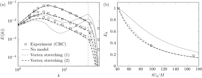
Figure 1: (a) Three-dimensional kinetic energy spectra as a function of computational wavenumber at the three measurement stations and (b) decay of the total normalized resolved kinetic energy, as obtained from large-eddy simulations of homogeneous isotropic turbulence on a $64^{3}$ grid. Results are shown for simulations without a subgrid-scale model (dotted line) and with the vortex-stretching-based eddy viscosity model, Eq. (55), with $C_{\mathrm{VS}}\approx 0.58$ (1) (dotted line) and $C_{\mathrm{VS}}\approx 0.68$ (2) (dash-dotted line). The experimental data from the experiment by Comte-Bellot and Corrsin (CBC) [6] are shown for reference (squares).

Fig. 1 shows the resulting energy spectra and the normalized total resolved kinetic energy. For comparison, the experimental data from the CBC experiment and results from large-eddy simulations without a model are provided. The resolved kinetic energy of the CBC experiment was estimated from discrete $64^{3}$ velocity fields with random phases that fit the three experimental energy spectra. A good match between results from the large-eddy simulation and experimental data is obtained. In fact, the vortex-stretching-based eddy viscosity model performs as least as good in simulations of homogeneous isotropic turbulence as Vreman’s model, Eq. 42. The currently obtained results, with $C_{\mathrm{VS}}\approx 0.68$, are practically indistinguishable from the energy spectra and decay of kinetic energy that are predicted by simulations using Vreman’s model with $C_{\mathrm{V}}\approx 0.27$ (not shown). Fig. 1 also provides an indication of the sensitivity of simulation results with respect to the model constant, $C_{\mathrm{VS}}$. A change in the model constant of more than 10%, from $C_{\mathrm{VS}}\approx 0.58$ to $C_{\mathrm{VS}}\approx 0.68$, still leads to a reasonable prediction of the three-dimensional kinetic energy spectra and a very satisfying prediction of the decay of kinetic energy.

5.2.2 Plane-channel flow

Next, we focus on large-eddy simulations of a turbulent plane-channel flow. The reference data for this test case come from the Direct Numerical Simulation (DNS) performed by Moser et al. [25]. Among other statistical quantities, these authors collected the mean velocity, $\langle u_{i}\rangle$, and the Reynolds stresses, $R_{ij}=\langle u_{i}u_{j}\rangle-\langle u_{i}\rangle\langle u_{j}\rangle$, where $\langle\cdot\rangle$ now indicates an average over time and the two homogeneous directions.

The large-eddy simulations were performed using the vortex-stretching-based eddy viscosity model, Eq. 55, and using Vreman’s model, Eq. 42. To match the reference data, a constant pressure gradient is prescribed to maintain a friction Reynolds number based on the wall shear stress of $Re_{\tau}\approx 590$. The domain size is taken to be $(L_{1},L_{2},L_{3})=(2\pi d,2d,\pi d)$, where $d$ represents the channel half-width. Again a $64^{3}$ grid is used, but here it is only taken to be uniform and periodic in the streamwise ($x_{1}$) and spanwise ($x_{3}$) directions, whereas the grid is stretched in the wall-normal direction ($x_{2}$). Because of the stretching and anisotropy of the grid, characterized by $\Delta x_{1}^{+}\approx 58$, $\Delta x_{2}^{+}\approx 2-61$ and $\Delta x_{3}^{+}\approx 29$, the subgrid characteristic length scale was defined according to Deardorff’s cube root of the cell volume, $\delta=(\Delta x_{1}\Delta x_{2}\Delta x_{3})^{1/3}$ [7].

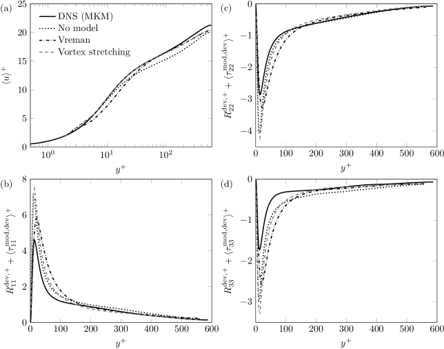
Figure 2: (a) Mean velocity profile and (b) streamwise, (c) wall-normal and (d) spanwise deviatoric Reynolds stresses compensated by the average model contribution, as obtained from large-eddy simulations of plane-channel flow at $Re_{\tau}\approx 590$ on a $64^{3}$ grid. Results are shown for simulations without a subgrid-scale model (dotted line), with Vreman’s model, Eq. (42), with $C_{\mathrm{V}}\approx 0.28$ (dash-dotted line) and with the vortex-stretching-based eddy viscosity model, Eq. (55), with $C_{\mathrm{VS}}\approx 0.55$ (dashed line). Results from Direct Numerical Simulation (DNS)[25] are shown for reference (solid line). All results are shown in wall units.

Figure 2 shows the mean velocity profile and the Reynolds stresses as obtained from the large-eddy simulations. The DNS data from Moser et al. [25] and a no-model large-eddy simulation are shown for reference. To allow for a fair comparison between the Reynolds stresses from the direct numerical simulation and from large-eddy simulations using traceless eddy viscosity models such as the vortex-stretching-based eddy viscosity model and Vreman’s model, we show only the deviatoric Reynolds stresses and compensate for the average model contribution [56]. All quantities are expressed in wall units, based on the friction velocity, $u_{\tau}$, and the channel half-width, $d$.

For the vortex-stretching-based eddy viscosity model, results are shown with $C_{\mathrm{VS}}\approx 0.55$. For this value of the model constant, which is remarkably close to $C_{\mathrm{VS}}\approx 0.58$ (the value that was obtained from matching the average model dissipation with that of the Smagorinsky model (see Section 5.2.1)), the mean velocity in the near-wall region is predicted very well. For Vreman’s model, results are shown with $C_{\mathrm{V}}\approx 0.28$, which is the value of the model constant for which the bulk velocity (the spatial average of the mean velocity) predicted by both subgrid-scale models is approximately equal. Vreman’s model fails to capture the behavior of the mean velocity near the wall. The mean velocity in the center of the channel is underpredicted by both models, but it is noted here that it seems to be a common deficiency of eddy viscosity models to not be able to predict the inflection of the mean velocity starting around $y^{+}\approx 100$. Note that both models are relatively robust when it comes to changes in the model constant. Changing $C_{\mathrm{VS}}$ or $C_{\mathrm{V}}$ by around 10% only causes a 1% change in the bulk velocity. For comparison, the simulations without a model had a 4% smaller bulk velocity than the simulations with a subgrid-scale model.

The Reynolds stress profiles show that both subgrid-scale models overpredict the streamwise stresses, while the other diagonal stresses are underpredicted. Again this seems to be a common feature of eddy viscosity models. Note, however, that Vreman’s model predicts Reynolds stresses with rather broad near-wall peaks, located too far from the wall, while the vortex-stretching-based eddy viscosity model predicts well the location and width of the near-wall peaks. The near-wall scaling behavior of both subgrid-scale models may explain these differences.

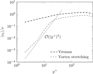
Figure 3: Average eddy viscosity in units of the kinematic viscosity, $\nu$, as obtained from large-eddy simulations of plane-channel flow at $Re_{\tau}\approx 590$ on a $64^{3}$ grid. Results are shown for simulations using the vortex-stretching-based eddy viscosity model, Eq. 55, with $C_{\mathrm{VS}}\approx 0.55$ (dashed line) and Vreman’s model, Eq. 42, with $C_{\mathrm{V}}\approx 0.28$ (dash-dotted line). The desired near-wall scaling behavior of the eddy viscosity is indicated (solid line).

The near-wall scaling of the vortex-stretching-based eddy viscosity model and of Vreman’s model is studied in Fig. 3, which shows the average eddy viscosity measured during the large-eddy simulations. The vortex-stretching-based eddy viscosity model exhibits the desired near-wall scaling, $\nu_{\mathrm{e}}=\mathcal{O}((y^{+})^{3})$, see Section 4.3, which ensures that the subgrid dissipation is not too large close to the wall. On the other hand, Vreman’s model shows a different near-wall scaling behavior, close to $\nu_{\mathrm{e}}=\mathcal{O}(y^{+})$, allowing for much higher values of eddy viscosity and, thus, a larger subgrid dissipation close to the wall. This may explain the problems Vreman’s model has with predicting the mean velocity and Reynolds stresses close to the wall. Improvements in the near-wall behavior of Vreman’s model may, however, also be obtained by using the original anisotropic implementation of the model [51], rather than the implementation of Eq. 42, which is based on an isotropic eddy viscosity with an anisotropic subgrid characteristic length scale, in this case given by Deardorff’s length scale [7].

In conclusion, we have seen how the model constraints of Section 3 can be used to derive new subgrid-scale models. An example of such a model, the vortex-stretching-based eddy viscosity model, Eq. 55, was tested in large-eddy simulations of homogeneous isotropic turbulence and a turbulent plane-channel flow. Good predictions of three-dimensional kinetic energy spectra and the decay of kinetic energy were obtained for the former test case, as well as for the mean velocity and Reynolds stresses in the latter test case. Although improvements are possible, in the form of a better prediction of the mean velocity in the center of the channel and the height of the near-wall peaks in the Reynolds stresses, we believe we have obtained encouraging results, that show the power of the framework of model constraints discussed in this work to design new subgrid-scale models with built-in desirable properties.

6 Summary

We studied the construction of subgrid-scale models for large-eddy simulation of incompressible turbulent flows. In particular, we aimed to consolidate a systematic approach of constructing subgrid-scale models. This approach is based on the idea that it is desirable that subgrid-scale models are consistent with important mathematical and physical properties of the Navier-Stokes equations and the turbulent stresses. We first discussed in detail several of these properties, namely: the symmetries of the Navier-Stokes equations, and the near-wall scaling behavior, realizability and dissipation properties of the turbulent stresses. In the last category we focused on Vreman’s study of the dissipation behavior of the turbulent stresses [51], the physical model requirements of Nicoud et al. [27], consistency with the second law of thermodynamics and Verstappen’s dissipation considerations relating to scale separation in large-eddy simulation [50, 49]. We furthermore outlined the requirements that subgrid-scale models have to satisfy in order to preserve these mathematical and physical properties.

As such, a framework of model constraints arose, that we subsequently applied to investigate the properties of existing subgrid-scale models. We focused specifically on the analysis of the behavior of subgrid-scale models that depend locally on the velocity gradient. These models satisfy some desired properties by construction, such as Galilean invariance and rotational invariance. Also, most subgrid-scale models of this form are consistent with the second law of thermodynamics. Other properties are only included in some of the existing models. For example, the WALE model [26], the $\sigma$ model [27] and the S3PQR models [45] have the proper near-wall scaling behavior, whereas the other models under study do not. The recently developed anisotropic minimum-dissipation (AMD) model [35] was designed to exhibit a particular dissipation behavior that leads to scale separation between large and small scales of motion, a property that is shared by some, but not all other models.

Thus, the subgrid-scale models that we considered do not generally satisfy all the desired properties. This can partly be understood from the fact that some model constraints, particularly dissipation properties, are not compatible with each other. We mentioned that the physical requirement of Nicoud et al. [27], that a model’s subgrid dissipation should vanish for all two-component flows, does not match with Vreman’s requirements derived from the mathematical properties of the turbulent stress tensor [51]. Also, Verstappen’s requirement for scale separation [50] can only be satisfied if a model has a nonzero subgrid dissipation for the pure axisymmetric strain, contrary to another requirement of Nicoud et al. [27]. We furthermore remarked that there seem to be some inherent limitations to subgrid-scale models that are based on the velocity gradient, as scaling invariance cannot be satisfied in the current formulation, where a length scale based on the local grid size is employed. Moreover, no velocity-gradient-based expression for the eddy viscosity was found that satisfies both of Vreman’s model requirements. This, however, may be due to our assumption of a filter that conforms to the symmetries of the Navier-Stokes equations (an isotropic filter) in computing the dissipation behavior of the true turbulent stresses. Despite these observations, we believe that there is room for improvement in the properties and, hence, the behavior of subgrid-scale models derived from the velocity gradient. The current work provides several suggestions in this way.

We showed how compatible model constraints can be combined to derive new subgrid-scale models that have desirable properties built into them. First, we illustrated how to construct a subgrid-scale model that is nonlinear in the velocity gradient, based on the invariants of the rate-of-strain tensor. Then we proposed a new eddy viscosity model based on the vortex stretching magnitude, to correct for the near-wall scaling and dissipation behavior of the Smagorinsky model. This new model has several interesting properties: it has the desired near-wall scaling behavior and it vanishes only in two-component flows, and in states of pure shear and pure rotation. This vortex-stretching-based eddy viscosity model was tested successfully in large-eddy simulations of decaying homogeneous isotropic turbulence and turbulent plane-channel flow.

With the current work we hope to have consolidated systematic approaches for the assessment of existing and the creation of new subgrid-scale models for large-eddy simulation. In future work, we would like to investigate in more detail constraints for the construction of subgrid-scale models. For example, incompatibilities between model requirements and the observation that even some very successful subgrid-scale models do not satisfy all the discussed requirements, warrant an assessment of the practical importance and significance of each of the model requirements. Furthermore, the fact that the velocity-gradient-based subgrid-scale models we considered here do not comply with scale invariance, calls for a detailed analysis of the symmetry preservation properties of the dynamic procedure [13], of other techniques that provide estimates of the turbulent kinetic energy and energy dissipation rate like the integral-length scale approximation [30, 34], and of flow-dependent definitions of the subgrid characteristic length scale in general. We would also like to investigate the behavior of subgrid-scale models that contain terms that are nonlinear in the rate-of-strain and rate-of-rotation tensors, particularly to study their ability to describe transport processes in flows. Finally, we will focus on devising new constraints for the construction of subgrid-scale models.

Acknowledgments

The authors thankfully acknowledge Professor Martin Oberlack for stimulating discussions during several stages of this project. Professor Michel Deville is kindly acknowledged for sharing his insights relating to nonlinear subgrid-scale models and realizability. Theodore Drivas and Perry Johnson are thankfully acknowledged for their valuable comments and criticisms on preliminary versions of this paper. Portions of this research have been presented at the 15th European Turbulence Conference, August 25-28th, 2015, Delft, The Netherlands, and at the 4th International Conference on Turbulence and Interactions, November 2nd-6th, 2015, Cargèse, Corsica, France. This work is part of the Free Competition in Physical Sciences, which is financed by the Netherlands Organisation for Scientific Research (NWO). M.H.S. gratefully acknowledges support from the Institute for Pure and Applied Mathematics (Los Angeles) for visits to the “Mathematics of Turbulence” program during the fall of 2014.

References

- [1] B. W. Anderson and J. A. Domaradzki “A subgrid-scale model for large-eddy simulation based on the physics of interscale energy transfer in turbulence” In Phys. Fluids 24, 2012 DOI: 10.1063/1.4729618
- [2] L. C. Berselli and T. Iliescu “A higher-order subfilter-scale model for large eddy simulation” In J. Comput. Appl. Math. 159, 2003, pp. 411–430 DOI: 10.1016/S0377-0427(03)00544-2
- [3] D. Carati, G. S. Winckelmans and H. Jeanmart “On the modelling of the subgrid-scale and filtered-scale stress tensors in large-eddy simulation” In J. Fluid Mech. 441, 2001, pp. 119–138 DOI: 10.1017/S0022112001004773
- [4] D. R. Chapman and G. D. Kuhn “The limiting behaviour of turbulence near a wall” In J. Fluid Mech. 170, 1986, pp. 265–292 DOI: 10.1017/S0022112086000885
- [5] R. A. Clark, J. H. Ferziger and W. C. Reynolds “Evaluation of subgrid-scale models using an accurately simulated turbulent flow” In J. Fluid Mech. 91, 1979, pp. 1–16 DOI: 10.1017/S002211207900001X
- [6] G. Comte-Bellot and S. Corrsin “Simple Eulerian time correlation of full- and narrow-band velocity signals in grid-generated, ‘isotropic’ turbulence” In J. Fluid Mech. 48, 1971, pp. 273–337 DOI: 10.1017/S0022112071001599
- [7] J. W. Deardorff “Numerical study of three-dimensional turbulent channel flow at large Reynolds numbers” In J. Fluid Mech. 41, 1970, pp. 453–480 DOI: 10.1017/S0022112070000691
- [8] M. O. Deville and T. B. Gatski “Mathematical Modeling for Complex Fluids and Flows” Springer Berlin Heidelberg, 2012 DOI: 10.1007/978-3-642-25295-2
- [9] R. Du Vachat “Realizability inequalities in turbulent flows” In Phys. Fluids 20, 1977, pp. 551–556 DOI: 10.1063/1.861911
- [10] U. Frisch “Turbulence: The Legacy of A. N. Kolmogorov” Cambridge: Cambridge University Press, 1995
- [11] C. Fureby and G. Tabor “Mathematical and Physical Constraints on Large-Eddy Simulations” In Theor. Comp. Fluid Dyn. 9, 1997, pp. 85–102 DOI: 10.1007/s001620050034
- [12] T. B. Gatski and T. Jongen “Nonlinear eddy viscosity and algebraic stress models for solving complex turbulent flows” In Prog. Aerosp. Sci. 36, 2000, pp. 655–682 DOI: 10.1016/S0376-0421(00)00012-9
- [13] M. Germano, U. Piomelli, P. Moin and W. H. Cabot “A dynamic subgrid-scale eddy viscosity model” In Phys. Fluids A 3, 1991, pp. 1760–1765 DOI: 10.1063/1.857955
- [14] S. Ghosal “Mathematical and Physical Constraints on Large-Eddy Simulation of Turbulence” In AIAA J. 37, 1999, pp. 425–433 DOI: 10.2514/2.752
- [15] H. S. Kang, S. Chester and C. Meneveau “Decaying turbulence in an active-grid-generated flow and comparisons with large-eddy simulation” In J. Fluid Mech. 480, 2003, pp. 129–160 DOI: 10.1017/S0022112002003579
- [16] B. Kosovic “Subgrid-scale modelling for the large-eddy simulation of high-Reynolds-number boundary layers” In J. Fluid Mech. 336, 1997, pp. 151–182 DOI: 10.1017/S0022112096004697
- [17] D. Kwak, W. C. Reynolds and J. H. Ferziger “Three-Dimensional, Time Dependent Computation of Turbulent Flow”, 1975
- [18] J. A. Langford and R. D. Moser “Optimal LES formulations for isotropic turbulence” In J. Fluid Mech. 398, 1999, pp. 321–346 DOI: 10.1017/S0022112099006369
- [19] A. Leonard “Energy Cascade in Large-Eddy Simulations of Turbulent Fluid Flows” In Turbulent Diffusion in Environmental Pollution: Proceedings of a Symposium held at Charlottesville, Virginia, April 8-14, 1973 18 A, Adv. Geophys. Academic Press, New York, 1974, pp. 237–248 DOI: 10.1016/S0065-2687(08)60464-1
- [20] J. L. Lumley “Computational Modeling of Turbulent Flows” 18, Adv. Appl. Mech. Elsevier, 1978, pp. 123–176 DOI: 10.1016/S0065-2156(08)70266-7
- [21] J. L. Lumley and G. R. Newman “The return to isotropy of homogeneous turbulence” In J. Fluid Mech. 82, 1977, pp. 161–178 DOI: 10.1017/S0022112077000585
- [22] T. S. Lund and E. A. Novikov “Parameterization of subgrid-scale stress by the velocity gradient tensor” Center for Turbulence Research, Stanford University, pp. 27–43 In Annual Research Briefs,, 1992
- [23] L. Marstorp, G. Brethouwer, O. Grundestam and A. V. Johansson “Explicit algebraic subgrid stress models with application to rotating channel flow” In J. Fluid Mech. 639, 2009, pp. 403–432 DOI: 10.1017/S0022112009991054
- [24] C. Meneveau and I. Marusic “Generalized logarithmic law for high-order moments in turbulent boundary layers” In J. Fluid Mech. 719, 2013, pp. R1 (11 pages) DOI: 10.1017/jfm.2013.61
- [25] R. D. Moser, J. Kim and N. N. Mansour “Direct numerical simulation of turbulent channel flow up to =590” In Phys. Fluids 11, 1999, pp. 943–945 DOI: 10.1063/1.869966
- [26] F. Nicoud and F. Ducros “Subgrid-scale stress modelling based on the square of the velocity gradient tensor” In Flow Turbul. Combust. 62, 1999, pp. 183–200 DOI: 10.1023/A:1009995426001
- [27] F. Nicoud, H. Baya Toda, O. Cabrit, S. Bose and J. Lee “Using singular values to build a subgrid-scale model for large eddy simulations” In Phys. Fluids 23, 2011 DOI: 10.1063/1.3623274
- [28] M. Oberlack “Invariant modeling in large-eddy simulation of turbulence” Center for Turbulence Research, Stanford University, pp. 3–22 In Annual Research Briefs,, 1997
- [29] M. Oberlack “Symmetries and Invariant Solutions of Turbulent Flows and their Implications for Turbulence Modelling” In Theories of Turbulence 442, International Centre for Mechanical Sciences Springer Vienna, 2002, pp. 301–366 DOI: 10.1007/978-3-7091-2564-9
- [30] U. Piomelli, A. Rouhi and B. J. Geurts “A grid-independent length scale for large-eddy simulations” In J. Fluid Mech. 766, 2015, pp. 499–527 DOI: 10.1017/jfm.2015.29
- [31] S. B. Pope “A more general effective-viscosity hypothesis” In J. Fluid Mech. 72, 1975, pp. 331–340 DOI: 10.1017/S0022112075003382
- [32] S. B. Pope “Turbulent Flows” Cambridge: Cambridge University Press, 2011
- [33] D. Razafindralandy, A. Hamdouni and M. Oberlack “Analysis and development of subgrid turbulence models preserving the symmetry properties of the Navier–Stokes equations” In Eur. J. Mech. B-Fluid. 26, 2007, pp. 531–550 DOI: 10.1016/j.euromechflu.2006.10.003
- [34] A. Rouhi, U. Piomelli and B. J. Geurts “Dynamic subfilter-scale stress model for large-eddy simulations” In Phys. Rev. Fluids 1, 2016, pp. 044401 DOI: 10.1103/PhysRevFluids.1.044401
- [35] W. Rozema, H. J. Bae, P. Moin and R. Verstappen “Minimum-dissipation models for large-eddy simulation” In Phys. Fluids 27, 2015, pp. 085107 DOI: 10.1063/1.4928700
- [36] P. Sagaut “Large Eddy Simulation for Incompressible Flows” Springer-Verlag Berlin Heidelberg, 2006 DOI: 10.1007/b137536
- [37] U. Schumann “Realizability of Reynolds-stress turbulence models” In Phys. Fluids 20, 1977, pp. 721–725 DOI: 10.1063/1.861942
- [38] M. H. Silvis and R. Verstappen “Constructing Physically-Consistent Subgrid-Scale Models for Large-Eddy Simulation of Incompressible Turbulent Flows” In Turbulence and Interactions: Proceedings of the TI 2015 Conference
- [39] M. H. Silvis and R. Verstappen “Physically-consistent subgrid-scale models for large-eddy simulation of incompressible turbulent flows”, 2015 arXiv:1510.07881 [physics.flu-dyn]
- [40] J. Smagorinsky “General circulation experiments with the primitive equations” In Mon. Weather Rev. 91, 1963, pp. 99–164 DOI: 10.1175/1520-0493(1963)091<0099:GCEWTP>2.3.CO;2
- [41] A. J. M. Spencer and R. S. Rivlin “The theory of matrix polynomials and its application to the mechanics of isotropic continua” In Arch. Ration. Mech. An. 2, 1958, pp. 309–336
- [42] A. J. M. Spencer and R. S. Rivlin “Isotropic integrity bases for vectors and second-order tensors. Part I.” In Arch. Ration. Mech. An. 9, 1962, pp. 45–63
- [43] C. G. Speziale “Galilean invariance of subgrid-scale stress models in the large-eddy simulation of turbulence” In J. Fluid Mech. 156, 1985, pp. 55–62 DOI: 10.1017/S0022112085001987
- [44] R. J. A. M. Stevens, M. Wilczek and C. Meneveau “Large-eddy simulation study of the logarithmic law for second- and higher-order moments in turbulent wall-bounded flow” In J. Fluid Mech. 757, 2014, pp. 888–907 DOI: 10.1017/jfm.2014.510
- [45] F. X. Trias, D. Folch, A. Gorobets and A. Oliva “Building proper invariants for eddy-viscosity subgrid-scale models” In Phys. Fluids 27, 2015, pp. 065103 DOI: 10.1063/1.4921817
- [46] R. W. C. P. Verstappen, W. Rozema and H. J. Bae “Numerical scale separation in large-eddy simulation” Center for Turbulence Research, Stanford University, pp. 417–426 In Proceedings of the Summer Program,, 2014
- [47] R. W. C. P. Verstappen and A. E. P. Veldman “Symmetry-preserving discretization of turbulent flow” In J. Comput. Phys. 187, 2003, pp. 343–368 DOI: 10.1016/S0021-9991(03)00126-8
- [48] R. W. C. P. Verstappen, S. T. Bose, J. Lee, H. Choi and P. Moin “A dynamic eddy-viscosity model based on the invariants of the rate-of-strain” Center for Turbulence Research, Stanford University, pp. 183–192 In Proceedings of the Summer Program,, 2010
- [49] R. Verstappen “How much eddy dissipation is needed to counterbalance the nonlinear production of small, unresolved scales in a large-eddy simulation of turbulence?” (to appear) In Comput. Fluids, 2016 DOI: 10.1016/j.compfluid.2016.12.016
- [50] Roel Verstappen “When Does Eddy Viscosity Damp Subfilter Scales Sufficiently?” In J. Sci. Comput. 49, 2011, pp. 94–110 DOI: 10.1007/s10915-011-9504-4
- [51] A. W. Vreman “An eddy-viscosity subgrid-scale model for turbulent shear flow: Algebraic theory and applications” In Phys. Fluids 16, 2004, pp. 3670–3681 DOI: 10.1063/1.1785131
- [52] B. Vreman, B. Geurts and H. Kuerten “Realizability conditions for the turbulent stress tensor in large-eddy simulation” In J. Fluid Mech. 278, 1994, pp. 351–362 DOI: 10.1017/S0022112094003745
- [53] B. Vreman, B. Geurts and H. Kuerten “Large-eddy simulation of the temporal mixing layer using the Clark model” In Theor. Comp. Fluid Dyn. 8, 1996, pp. 309–324 DOI: 10.1007/BF00639698
- [54] B.-C. Wang and D. J. Bergstrom “A dynamic nonlinear subgrid-scale stress model” In Phys. Fluids 17, 2005, pp. 035109 DOI: 10.1063/1.1858511
- [55] I. Wendling and M. Oberlack “On the Investigation of a Dynamic Nonlinear Subgrid-Scale Model” In Complex Effects in Large Eddy Simulations 56, Lecture Notes in Computational Science and Engineering Springer Berlin Heidelberg, 2007, pp. 89–97 DOI: 10.1007/978-3-540-34234-2_7
- [56] G. S. Winckelmans, H. Jeanmart and D. Carati “On the comparison of turbulence intensities from large-eddy simulation with those from experiment or direct numerical simulation” In Phys. Fluids 14, 2002, pp. 1809–1811 DOI: 10.1063/1.1466824
- [57] G. S. Winckelmans, A. A. Wray, O. V. Vasilyev and H. Jeanmart “Explicit-filtering large-eddy simulation using the tensor-diffusivity model supplemented by a dynamic Smagorinsky term” In Phys. Fluids 13, 2001, pp. 1385–1403 DOI: 10.1063/1.1360192