An application of Hoffman graphs for spectral characterizations of graphs

Abstract

In this paper, we present the first application of Hoffman graphs for spectral characterizations of graphs. In particular, we show that the $2$-clique extension of the $(t+1)\times(t+1)$-grid is determined by its spectrum when $t$ is large enough. This result will help to show that the Grassmann graph $J_{2}(2D,D)$ is determined by its intersection numbers as a distance regular graph, if $D$ is large enough.
Keywords: Hoffman graph, graph eigenvalue, interlacing, walk-regular, spectral characterizations.
2010 Math. Subj. Class.: 05C50, 05C75.

1 Introduction

Bang, Van Dam and Koolen [2] showed that the Hamming graphs $H(3,q)$ are determined by their spectrum if $q\geq 36$. In this paper, we will show a similar result for the $2$-clique extension of the square grid. (For definitions we refer the reader to the next section.) In this paper we will show the following result:

Theorem 1.1.

Let $G$ be a graph with spectrum

$$\big{\{}(4t+1)^{1},\leavevmode\nobreak\ (2t-1)^{2t},\leavevmode\nobreak\ (-1)^{(t+1)^{2}},\leavevmode\nobreak\ (-3)^{t^{2}}\big{\}}.$$

Then there exists a positive constant $C$ such that if $t\geq C$, then $G$ is the $2$-clique extension of the $(t+1)\times(t+1)$-grid.

Remark 1.2.

The current estimates for $C$ are unrealistic high, since the proof implicitly uses Ramsey theory.

In [1] it was shown that the $2$-coclique extension of the square grid is usually not determined by its spectrum.

A motivation came from the study of Grassmann graphs. Gavrilyuk and Koolen studied [8] the question whether the Grassmann graph $J_{2}(2D,D)$ is determined as a distance-regular graph by its intersection numbers. (For definitions of distance-regular graphs and related notions we refer to [3] and [7].) They showed that for any vertex, the subgraph induced by the neighbours of this vertex has the spectrum of the $2$-clique extension of a certain square grid. They used the main theorem of this paper to show that the Grassmann graph $J_{2}(2D,D)$ is determined as a distance-regular graph by its intersection numbers, if $D$ is large enough.

Another motivation for studying the $2$-clique extension of the $(t+1)\times(t+1)$-grid is because this is a connected regular graph with four distinct eigenvalues. Regular graphs with four distinct eigenvalues have been previously studied [4], and a key observation that we will use is that these graphs are walk-regular, which implies strong combinatorial information on the graph.

The starting point for our work is a result by Koolen et al. [14]:

Theorem 1.3.

[14] There exists a positive integer $t$ such that any graph, that is cospectral with the $2$-clique extension of $(t_{1}\times t_{2})$-grid is the slim graph of a $2$-fat $\big{\{}$,,$\big{\}}$-line Hoffman graph for all $t_{1}\geq t_{2}\geq t$.

As a direct consequence, we obtain the following corollary:

Corollary 1.4.

There exists a positive integer $T$ such that any graph, that is cospectral with the $2$-clique extension of $(t+1)\times(t+1)$-grid is the slim graph of a $2$-fat $\big{\{}$,,$\big{\}}$-line Hoffman graph for all $t\geq T$.

In view of Corollary 1.4, our Theorem 1.1 will follow from the following result:

Theorem 1.5.

Let $G$ be a graph cospectral with the $2$-clique extension of the $(t+1)\times(t+1)$-grid. If $G$ is the slim graph of a $2$-fat $\big{\{}$,,$\big{\}}$-line Hoffman graph, then $G$ is the $2$-clique extension of the $(t+1)\times(t+1)$-grid when $t>4$.

The main focus of this paper is to prove Theorem 1.5, and it is organized as follows. In Section 2, we review some preliminaries on graphs, interlacing and Hoffman graphs. Section 3 considers the graph cospectral with the $2$-clique extension of the $(t+1)\times(t+1)$-grid, which is the slim graph of the Hoffman graph having possible indecomposable factors isomorphic to the Hoffman graphs in Figure 3. In Section 4, we forbid two of the mentioned Hoffman graphs to occur as indecomposable factors. In Section 5, the order of the quasi-cliques of the possible indecomposable factors is determined. Finally, in Section 6, we finish the proof of Theorem 1.5.

2 Preliminaries

Throughout this paper we will consider only undirected graphs without loops or multiple edges. Suppose that $\Gamma$ is a graph with vertex set $V(\Gamma)$ with $|V(\Gamma)|=n$ and edge set $E(\Gamma)$. Let $A$ be the adjacency matrix of $\Gamma$, then the eigenvalues of $\Gamma$ are the eigenvalues of $A$. Let $\lambda_{0},\lambda_{1},\ldots,\lambda_{t}$ be the distinct eigenvalues of $\Gamma$ and $m_{i}$ be the multiplicity of $\lambda_{i}$ ($i=0,1,\ldots,t$). Then the multiset $\{\lambda_{0}^{m_{0}},\lambda_{1}^{m_{1}},\ldots,\lambda_{t}^{m_{t}}\}$ is called the spectrum of $\Gamma$.

Two graphs are called cospectral if they have the same spectrum.

For a vertex $x$, let $\Gamma_{i}(x)$ be the set of vertices at distance $i$ from $x$. When $i=1$, we also denote it by $N_{\Gamma}(x)$. For two distinct vertices $x$ and $y$, we denote the number of common neighbors between them by $\lambda_{x,y}$ if $x$ and $y$ are adjacent, and by $\mu_{x,y}$ if they are not.

Recall that the Kronecker product $M_{1}\otimes M_{2}$ of two matrices $M_{1}$ and $M_{2}$ is obtained by replacing the $ij$-entry of $M_{1}$ by $({M_{1}})_{ij}M_{2}$ for all $i$ and $j$. If $\tau$ and $\theta$ are eigenvalues of $M_{1}$ and $M_{2}$, then $\tau\theta$ is an eigenvalue of $M_{1}\otimes M_{2}$ [9].

Recall that a ($c$)-clique (or complete graph) is a graph (on $c$ vertices) in which every pair of vertices is adjacent.

For an integer $q\geq 1$, the $q$-clique extension of $\Gamma$ is the graph $\widetilde{\Gamma}$ obtained from $\Gamma$ by replacing each vertex $x\in V(\Gamma)$ by a clique $\widetilde{X}$ with $q$ vertices, such that $\tilde{x}\sim\tilde{y}$ (for $\tilde{x}\in\widetilde{X},\leavevmode\nobreak\ \tilde{y}\in\widetilde{Y},\leavevmode\nobreak\ \widetilde{X}\neq\widetilde{Y}$) in $\widetilde{\Gamma}$ if and only if $x\sim y$ in $\Gamma$. If $\widetilde{\Gamma}$ is the $q$-clique extension of $\Gamma$, then $\widetilde{\Gamma}$ has adjacency matrix $J_{q}\otimes(A+I_{n})-I_{qn}$, where $J_{q}$ is the all one matrix of size $q$ and $I_{n}$ is the identity matrix of size $n$.

In particular, if $q=2$ and $\Gamma$ has spectrum

$$\big{\{}\lambda_{0}^{m_{0}},\lambda_{1}^{m_{1}},\ldots,\lambda_{t}^{m_{t}}\big{\}},$$ (1)

then it follows that the spectrum of $\widetilde{\Gamma}$ is

$$\big{\{}(2\lambda_{0}+1)^{m_{0}},(2\lambda_{1}+1)^{m_{1}},\ldots,(2\lambda_{t}+1)^{m_{t}},(-1)^{(m_{0}+m_{1}+\cdots+m_{t})}\big{\}}.$$ (2)

In case that $\Gamma$ is a connected regular graph with valency $k$ and with adjacency matrix $A$ having exactly four distinct eigenvalues $\{\lambda_{0}=k,\lambda_{1},\lambda_{2},\lambda_{3}\}$, then $A$ satisfies the following (see for example [12]):

$$A^{3}-\left(\displaystyle\sum_{i=1}^{3}\lambda_{i}\right)A^{2}+\left(\displaystyle\sum_{1\leq i<j\leq 3}\lambda_{i}\lambda_{j}\right)A-\lambda_{1}\lambda_{2}\lambda_{3}I=\frac{\prod_{i=1}^{3}(k-\lambda_{i})}{n}J.$$ (3)

We also need to introduce an important spectral tool that will be used throughout this paper: eigenvalue interlacing.

Lemma 2.1.

[11, Interlacing] Let $A$ be a real symmetric $n\times n$ matrix with eigenvalues $\lambda_{1}\geq\cdots\geq\lambda_{n}$. For some $m<n$, let $S$ be a real $n\times m$ matrix with orthonormal columns, $S^{T}S=I$, and consider the matrix $B=S^{T}AS$, with eigenvalues $\mu_{1}\geq\cdots\geq\mu_{m}$. Then,

• the eigenvalues of $B$ interlace those of $A$, that is,

  $$\lambda_{i}\geq\mu_{i}\geq\lambda_{n-m+i},\qquad i=1,\ldots,m.$$ (4)

• if there exists an integer $j\in\{1,2,\ldots,m\}$ such that $\lambda_{i}=\mu_{i}$ for $1\leq i\leq j$ and $\lambda_{n-m+i}=\mu_{i}$ for $j+1\leq i\leq m$, then the interlacing is tight and $SB=AS$.

Two interesting particular cases of interlacing are obtained by choosing appropriately the matrix $S$. If $S=\left(\begin{array}[]{cc}I&O\\ O&O\\ \end{array}\right)$, then $B$ is just a principal submatrix of $A$. If $\pi=\{V_{1},\ldots,V_{m}\}$ is a partition of the vertex set $V$, with each $V_{i}\neq\emptyset$, we can take for $\widetilde{B}$ the so-called quotient matrix of $A$ with respect to $\pi$. Let $A$ be partitioned according to $\pi$:

$$A=\left(\begin{array}[]{ccc}A_{1,1}&\cdots&A_{1,m}\\ \vdots&&\vdots\\ A_{m,1}&\cdots&A_{m,m}\end{array}\right),$$

where $A_{i,j}$ denotes the submatrix (block) of $A$ formed by rows in $V_{i}$ and columns in $V_{j}$. The characteristic matrix $C$ is the $n\times m$ matrix whose $j^{\text{th}}$ column is the characteristic vector of $V_{j}$ ($j=1,\ldots,m$).

Then, the quotient matrix of $A$ with respect to $\pi$ is the $m\times m$ matrix $\widetilde{B}$ whose entries are the average row sums of the blocks of $A$, more precisely:

$$(\widetilde{B})_{i,j}=\frac{1}{|V_{i}|}(C^{T}AC)_{i,j}.$$

The partition $\pi$ is called equitable (or regular) if each block $A_{i,j}$ of $A$ has constant row (and column) sum, that is, $C\widetilde{B}=AC$.

Lemma 2.2.

Suppose $\widetilde{B}$ is the quotient matrix of a symmetric partitioned matrix $A$.

The eigenvalues of $\widetilde{B}$ interlace the eigenvalues of $A$.

If the interlacing is tight, then the partition $\pi$ is equitable.

Lemma 2.3.

[9, Theorem $9.3.3$] If $\pi$ is an equitable partition of a graph $\Gamma$, then the characteristic polynomial of $\widetilde{B}$ divides the characteristic polynomial of $A$.

2.1 Hoffman graphs

We will need the following properties and definitions related to Hoffman graphs.

Definition 2.4.

A Hoffman graph $\mathfrak{h}$ is a pair $(H,\mu)$ of a graph $H=(V,E)$ and a labeling map $\mu:V\rightarrow\{f,s\}$, satisfying the following conditions:

• every vertex with label $f$ is adjacent to at least one vertex with label $s$;

• vertices with label $f$ are pairwise non-adjacent.

We call a vertex with label $s$ a slim vertex, and a vertex with label $f$ a fat vertex. We denote by $V_{s}=V_{s}(\mathfrak{h})$ (resp. $V_{f}(\mathfrak{h})$) the set of slim (resp. fat) vertices of $\mathfrak{h}$.

For a vertex $x$ of $\mathfrak{h}$, we define $N_{\mathfrak{h}}^{s}(x)$ (resp. $N_{\mathfrak{h}}^{f}(x)$) the set of slim (resp. fat) neighbors of $x$ in $\mathfrak{h}$. If every slim vertex of a Hoffman graph $\mathfrak{h}$ has a fat neighbor, then we call $\mathfrak{h}$ fat. And if every slim vertex has at least $t$ fat neighbors, we call $\mathfrak{h}$ $t$-fat. In a similar fashion, we define $N^{f}(x_{1},x_{2})=N^{f}_{\mathfrak{h}}(x_{1},x_{2})$ to be the set of common fat neighbors of two slim vertices $x_{1}$ and $x_{2}$ in $\mathfrak{h}$ and $N^{s}(F_{1},F_{2})=N^{s}_{\mathfrak{h}}(F_{1},F_{2})$ to be the set of common slim neighbors of two fat vertices $F_{1}$ and $F_{2}$ in $\mathfrak{h}$.

The slim graph of a Hoffman graph $\mathfrak{h}$ is the subgraph of $H$ induced by $V_{s}(\mathfrak{h})$.

A Hoffman graph $\mathfrak{h_{1}}=(H_{1},\mu_{1})$ is called an induced Hoffman subgraph of $\mathfrak{h}=(H,\mu)$, if $H_{1}$ is an induced subgraph of $H$ and $\mu_{1}(x)=\mu(x)$ for all vertices $x$ of $H_{1}$.

Let $W$ be a subset of $V_{s}(\mathfrak{h})$. An induced Hoffman subgraph of $\mathfrak{h}$ generated by $W$, denoted by $\langle W\rangle_{\mathfrak{h}}$, is the Hoffman subgraph of $\mathfrak{h}$ induced by $W\bigcup\{f\in V_{f}(\mathfrak{h})\leavevmode\nobreak\ |f\sim w\text{ for some }w\in W\}$.

A quasi-clique is a subgraph of the slim graph of $\mathfrak{h}$ induced by the neighborhood of a fat vertex of $\mathfrak{h}$. If a quasi-clique is induced by the neighborhood of fat vertex $F$, we say it is the quasi-clique corresponding to $F$ and denote it by $Q_{\mathfrak{h}}(F)$.

Definition 2.5.

For a Hoffman graph $\mathfrak{h}=(H,\mu)$, let $A$ be the adjacency matrix of $H$

$$A=\left(\begin{array}[]{cc}A_{s}&C\\ C^{T}&O\end{array}\right)$$

in a labeling in which the fat vertices come last. The special matrix $\mathcal{S}(\mathfrak{h})$ of $\mathfrak{h}$ is the real symmetric matrix $\mathcal{S}(\mathfrak{h}):=A_{s}-CC^{T}.$ The eigenvalues of $\mathfrak{h}$ are the eigenvalues of $\mathcal{S}(\mathfrak{h})$.

Note that $\mathfrak{h}$ is not determined by $\mathcal{S}$, since different $\mathfrak{h}$ may have the same special matrix $\mathcal{S}$. Observe also that if there are not fat vertices, then $\mathcal{S}(\mathfrak{h})=A_{s}$ is just the standard adjacency matrix.

Now we introduce two key concepts in this work: the direct sum of Hoffman graphs and line Hoffman graphs.

Definition 2.6.

(Direct sum of Hoffman graphs) Let $\mathfrak{h}$ be a Hoffman graph and $\mathfrak{h}^{1}$ and $\mathfrak{h}^{2}$ be two induced Hoffman subgraphs of $\mathfrak{h}$. The Hoffman graph $\mathfrak{h}$ is the direct sum of $\mathfrak{h}^{1}$ and $\mathfrak{h}^{2}$, that is $\mathfrak{h}=\mathfrak{h}^{1}\bigoplus\mathfrak{h}^{2}$, if and only if $\mathfrak{h}^{1},\mathfrak{h}^{2}$ and $\mathfrak{h}$ satisfy the following conditions:

• $V(\mathfrak{h})=V(\mathfrak{h}^{1})\bigcup V(\mathfrak{h}^{2});$

• $\big{\{}V_{s}(\mathfrak{h}^{1}),V_{s}(\mathfrak{h}^{2})\big{\}}$ is a partition of $V_{s}(\mathfrak{h})$;

• if $x\in V_{s}(\mathfrak{h}^{i})$, $f\in V_{f}(\mathfrak{h})$ and $x\sim f$, then $f\in V_{f}(\mathfrak{h}^{i})$;

• if $x\in V_{s}(\mathfrak{h}^{1})$ and $y\in V_{s}(\mathfrak{h}^{2})$, then $x$ and $y$ have at most one common fat neighbor, and they have exactly one common fat neighbor if and only if they are adjacent.

Let us show an example of how to construct a direct sum of two Hoffman graphs.

Example 2.7.

Let $\mathfrak{h}_{1},\mathfrak{h}_{2}$ and $\mathfrak{h}_{3}$ be the Hoffman graphs represented in Figure 1.

[] [] [1.2]

$\mathfrak{h}_{1}$

$\mathfrak{h}_{2}$

$\mathfrak{h}_{3}$

Figure 1:

Then $\mathfrak{h}_{1}\bigoplus\mathfrak{h}_{2},$ $\mathfrak{h}_{1}\bigoplus\mathfrak{h}_{3}$ and $\mathfrak{h}_{2}\bigoplus\mathfrak{h}_{3}$ are shown in Figure 2.

[1.0] [1.0] [1.2]

$\mathfrak{h}_{1}\bigoplus\mathfrak{h}_{2}$

$\mathfrak{h}_{1}\bigoplus\mathfrak{h}_{3}$

$\mathfrak{h}_{2}\bigoplus\mathfrak{h}_{3}$

Figure 2:

Definition 2.8.

If a Hoffman graph $\mathfrak{h}$ is the direct sum of Hoffman graphs $\mathfrak{h}_{1}$ and $\mathfrak{h}^{\prime}$, then we call the Hoffman graph $\mathfrak{h}_{1}$ a factor of $\mathfrak{h}$. If $\mathfrak{h}_{1}$ is indecomposable, then it is called indecomposable.

Definition 2.9.

Let $\mathfrak{G}$ be a family of Hoffman graphs. A Hoffman graph $\mathfrak{h}$ is called a $\mathfrak{G}$-line Hoffman graph if $\mathfrak{h}$ is an induced Hoffman subgraph of Hoffman graph $\mathfrak{h}^{\prime}=\oplus_{i=1}^{r}\mathfrak{h}_{i}^{\prime}$ where $\mathfrak{h}_{i}^{\prime}$ is isomorphic to an induced Hoffman subgraph of some Hoffman graph in $\mathfrak{G}$ for $i=1,\dots,r$, such that $\mathfrak{h}^{\prime}$ has the same slim graph as $\mathfrak{h}$.

3 Cospectral graph with the $2$-clique extension of the $(t+1)\times(t+1)$-grid

In this section, we study some consequences of Theorem 1.3. As mentioned in Section 1, the main goal of this paper is to show Theorem 1.5. Therefore, from now on we shall prepare the proof for Theorem 1.5.
Let $t>0$ and for the rest of this paper, let $G$ be a graph cospectral with the $2$-clique extension of the $(t+1)\times(t+1)$-grid with adjacency matrix $A$. Since $G$ has the same spectrum as the $2$-clique extension of the $(t+1)\times(t+1)$-grid, $G$ is a regular graph with valency $k=4t+1$ and spectrum

$$\big{\{}\eta_{0}^{m_{0}},\eta_{1}^{m_{1}},\eta_{2}^{m_{2}},\eta_{3}^{m_{3}}\big{\}}=\big{\{}(4t+1)^{1},\leavevmode\nobreak\ (2t-1)^{2t},\leavevmode\nobreak\ (-1)^{(t+1)^{2}},\leavevmode\nobreak\ (-3)^{t^{2}}\big{\}}.$$

Using (3) we obtain

$$A^{3}+(5-2t)A^{2}+(7-8t)A+(3-6t)I=(16t+8)J.$$

Thus, we have

$$A^{3}_{(x,y)}=\left\{\begin{array}[]{l l}8t^{2}+4t,&\text{if }x=y;\\ 24t+1-(5-2t)\lambda_{x,y},&\text{if }x\sim y;\\ 16t+8-(5-2t)\mu_{x,y},&\text{if }x\not\sim y.\end{array}\right.$$ (6)

If $G$ is the slim graph of a $2$-fat $\big{\{}$,,$\big{\}}$-line Hoffman graph, then there exists a $2$-fat Hoffman graph $\mathfrak{h}$, such that $\mathfrak{h}=\bigoplus_{i=1}^{s}\mathfrak{h}_{i}$ with slim graph $G$, and $\mathfrak{h}_{i}$ is isomorphic to one of the Hoffman graphs in the set $\mathfrak{G}=\big{\{}$,,,, ,,$\big{\}}$ for $i=1,\ldots,s$.

We will now exclude two Hoffman graphs from the set $\mathfrak{G}$. To do so, we note the following remark:

Remark 3.1.

The Hoffman graph has the same slim graph as .

The Hoffman graph has the same slim graph as , which is the direct sum of two Hoffman graphs isomorphic to with one common fat neighbor (see Example 2.7).

Remark 3.1 implies that we may assume that the $2$-fat Hoffman graph $\mathfrak{h}$, introduced before Remark 3.1, satisfies the following property, by adding fat vertices, if necessary.

Property 3.2.

$\mathfrak{h}$ has $G$ as slim graph;

$\mathfrak{h}=\bigoplus_{i=1}^{s^{\prime}}\mathfrak{h}_{i}^{\prime}$, where $\mathfrak{h}_{i}^{\prime}$ isomorphic to one of the Hoffman graphs shown in Figure 3, for $i=1,\ldots,s^{\prime}$.

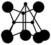
[0.8] [1.2] [0.8] [0.8] [0.8]

$\mathfrak{g}_{1}$

$\mathfrak{g}_{2}$

$\mathfrak{g}_{3}$

$\mathfrak{g}_{4}$

$\mathfrak{g}_{5}$

Figure 3:

Using Property 3.2 and the definition of direct sum, we obtain the following lemma:

Lemma 3.3.

Any two distinct fat vertices $F_{1}$ and $F_{2}$ of $\mathfrak{h}$ have at most two common slim neighbors, i.e., $|N^{s}_{\mathfrak{h}}(F_{1},F_{2})|\leq 2$, and if $F_{1}$ and $F_{2}$ have exactly two common slim neighbors $x_{1}$ and $x_{2}$, then $x_{1}$ and $x_{2}$ are adjacent. In particular, this means that in this case, is an indecomposable factor of $\mathfrak{h}$.

If is an induced Hoffman subgraph of one of the $\mathfrak{h_{i}}$ of Figure 3, and $\mathfrak{h_{i}}\not\backsimeq$ , then $F_{1}$ and $F_{2}$ have exactly one slim common neighbor in $\mathfrak{h}$.

Proof.

($i$) Suppose that $N^{s}_{\mathfrak{h}}(F_{1},F_{2})=\{x_{1},x_{2},\ldots,x_{p}\}$. By Definition 2.6 $(iv)$, we find that these $p$ distinct slim vertices and two fat vertices should be in the same indecomposable factor of $\mathfrak{h}$. By Figure 3, we see that if $p\geq 2$, then $p=2$ and the only indecomposable factor is (isomorphic to) $\mathfrak{g}_{4}$.

($ii$) This follows from ($i$). ∎

4 Forbidding factors $\mathfrak{g_{1}}$ and $\mathfrak{g_{2}}$

In this section, we will show that $\mathfrak{g}_{1}$ and $\mathfrak{g}_{2}$ can not occur as an indecomposable factor of $\mathfrak{h}$. For this, we first need the following lemma:

Lemma 4.1.

Any two distinct nonadjacent vertices $x$ and $y$ in $G$ have at most $2t+2$ common neighbors, that is, $\mu_{x,y}\leq 2t+2$.

Proof.

Define a matrix $M$ as follows:

$$\begin{split}M&=(A-\eta_{1}I)(A-\eta_{2}I)\\ &=(A-(2t-1)I)(A+I)\\ &=A^{2}-2(t-1)A-(2t-1)I.\end{split}$$ (7)

Then $M$ is positive semidefinite (as $A$ has no eigenvalues between $\eta_{1}$ and $\eta_{2}$), and we have

$$M_{(x,y)}=\left\{\begin{array}[]{l l}k-(2t-1)=2t+2,&\text{if }x=y;\\ -2(t-1)+\lambda_{x,y},&\text{if }x\sim y;\\ \mu_{x,y},&\text{if }x\not\sim y.\end{array}\right.$$ (8)

Since $M$ is positive semidefinite, all its principal submatrices are positive semidefinite. Let $x$ and $y$ be two distinct nonadjacent vertices of $G$. Then

$$\left(\begin{array}[]{cc}2t+2&\mu_{x,y}\\ \mu_{x,y}&2t+2\end{array}\right)$$

is positive semidefinite and hence $\mu_{x,y}\leq 2t+2$ holds. ∎

Using Lemma 4.1, we obtain the following result:

Lemma 4.2.

The Hoffman graph $\mathfrak{g}_{1}$ can not be an indecomposable factor of $\mathfrak{h}$ when $t>1$.

The Hoffman graph $\mathfrak{g}_{2}$ can not be an indecomposable factor of $\mathfrak{h}$ when $t>1$.

Proof.

$(i)$ Suppose that $\mathfrak{g}_{1}$ is an indecomposable factor of $\mathfrak{h}$, where $a_{i}=|V(Q_{\mathfrak{h}}(F_{i}))|$, as shown in Figure 4.

Figure 4: $\mathfrak{g}_{1}$

By Lemma 3.3, we find that $N^{s}_{\mathfrak{h}}(F_{1},F_{2})=\{x_{1}\},N^{s}_{\mathfrak{h}}(F_{2},F_{3})=\{x_{2}\},\leavevmode\nobreak\ N^{s}_{\mathfrak{h}}(F_{1},F_{4})=\{x_{4}\},\leavevmode\nobreak\ |N^{s}_{\mathfrak{h}}(F_{1},F_{3})|\leq 2,$ and $|N^{s}_{\mathfrak{h}}(F_{2},F_{4})|\leq 2.$ By the definition of direct sum, we know that if a vertex $x$ ($x\neq x_{3}$) is adjacent to $x_{1}$ in $G$, then $x\in N^{s}_{\mathfrak{h}}(F_{1})$ or $x\in N^{s}_{\mathfrak{h}}(F_{2})$. So $a_{1}+a_{2}-3=a_{1}-2+a_{2}-2+1=|N_{G}(x_{1})|=k=4t+1$, that is $a_{1}+a_{2}=4t+4$. (In a similar way, we obtain that $a_{2}+a_{3}=a_{3}+a_{4}=a_{1}+a_{4}=4t+4$, so $a_{1}=a_{3}$ and $a_{2}=a_{4}$.) Note that $\mu_{x_{1},x_{2}}=a_{2}-2+|N^{s}_{\mathfrak{h}}(F_{1},F_{3})|,\leavevmode\nobreak\ \mu_{x_{1},x_{4}}=a_{1}-2+|N^{s}_{\mathfrak{h}}(F_{2},F_{4})|,$ $\lambda_{x_{2},x_{4}}=|N^{s}_{\mathfrak{h}}(F_{1},F_{3})|+|N^{s}_{\mathfrak{h}}(F_{2},F_{4})|.$ We obtain

$$\mu_{x_{1},x_{2}}+\mu_{x_{1},x_{4}}=4t+\lambda_{x_{2},x_{4}}.$$ (9)

Without loss of generality, we may assume that $\mu_{x_{1},x_{4}}\leq\mu_{x_{1},x_{2}}$. From Lemma 4.1 and Equation (9), we obtain

$$0\leq\lambda_{x_{2},x_{4}}\leq 4,\quad\mu_{x_{1},x_{4}}\leq\mu_{x_{1},x_{2}}\leq 2t+2,$$ (10)

$$\text{and }2t-2+\lambda_{x_{2},x_{4}}\leq\mu_{x_{1},x_{4}}\leq 2t+\bigg{\lfloor}\frac{\lambda_{x_{2},x_{4}}}{2}\bigg{\rfloor}.$$

Take the positive semidefinite principal submatrix $M_{1}$ of $M$, corresponding to the vertices $\{x_{1},x_{2},x_{4}\}$. Then, we obtain (by using (8)):

$$M_{1}=\begin{pmatrix}2t+2&\mu_{x_{1},x_{2}}&\mu_{x_{1},x_{4}}\\ \mu_{x_{1},x_{2}}&2t+2&-2(t-1)+\lambda_{x_{2},x_{4}}\\ \mu_{x_{1},x_{4}}&-2(t-1)+\lambda_{x_{2},x_{4}}&2t+2\end{pmatrix}.$$

Replacing $\mu_{x_{1},x_{4}}$ by $\mu$ and $\lambda_{x_{2},x_{4}}$ by $\lambda$ and using (9), we have

$$M_{1}=\begin{pmatrix}2t+2&4t+\lambda-\mu&\mu\\ 4t+\lambda-\mu&2t+2&-2(t-1)+\lambda\\ \mu&-2(t-1)+\lambda&2t+2\end{pmatrix}.$$

The above matrix $M_{1}$ has determinant

$$\begin{split}det(M_{1})=&-32t^{3}-8\lambda t^{2}+\big{(}(8\lambda+32)\mu-4\lambda^{2}-16\lambda+32\big{)}t\\ &-(2\lambda+8)\mu^{2}+(2\lambda^{2}+8\lambda)\mu-4\lambda^{2}-8\lambda,\end{split}$$

where $0\leq\lambda\leq 4,\leavevmode\nobreak\ 2t-2+\lambda\leq\mu\leq 2t+\lfloor\frac{\lambda}{2}\rfloor$ (by (10)).

If $t>1$, by checking all the possible values of $\lambda$ and $\mu$, we obtain that $\text{det}(M_{1})<0$ and this is impossible since $M_{1}$ is positive semidefinite.

$(ii)$ can be shown in a similar way. Suppose that $\mathfrak{g}_{2}$ is an indecomposable factor of $\mathfrak{h}$, where $a_{i}=|V(Q_{\mathfrak{h}}(F_{i}))|$, as shown in Figure 5.

Figure 5: $\mathfrak{g}_{2}$

Then the submatrix $M_{1}$ is replaced by

$$M_{2}=\begin{pmatrix}2t+2&4t+1+\lambda-\mu&\mu\\ 4t+1+\lambda-\mu&2t+2&-2(t-1)+\lambda\\ \mu&-2(t-1)+\lambda&2t+2\end{pmatrix},$$

with determinant:

$$\begin{split}det(M_{2})=&-32t^{3}-(8\lambda+16)t^{2}+\big{(}(8\lambda+32)\mu-4\lambda^{2}-20\lambda+14\big{)}t\\ &-(2\lambda+8)\mu^{2}+(2\lambda^{2}+10\lambda+8)\mu-4\lambda^{2}-12\lambda-2,\end{split}$$

where $0\leq\lambda=\lambda_{x_{2},x_{4}}\leq 4$ and $2t-1+\lambda\leq\mu=\mu_{x_{1},x_{4}}\leq 2t+\lfloor\frac{1+\lambda}{2}\rfloor$.

If $t>1$, by checking all the possible values of $\lambda$ and $\mu$, we obtain that $\text{det}(M_{2})<0$ and the result follows, as this gives a contradiction. ∎

5 The order of quasi-cliques

5.1 An upper bound on the order of quasi-cliques

From the above section, we find that the only possible indecomposable factors of $\mathfrak{h}$ are $\mathfrak{g}_{3}$, $\mathfrak{g}_{4}$ and $\mathfrak{g}_{5}$.

Proposition 5.1.

Let $q$ be the order of a quasi-clique $Q$ corresponding to a fat vertex $F$ in $\mathfrak{h}$. Then $q\leq 2t+2$ when $t>1$.

Proof.

We show the following three claims from which the proposition follows.

Claim 5.2.

In the quasi-clique $Q$, every vertex has valency at least $q-2$.

Proof.

If there exists a vertex that has two nonneighbors in $Q$, then in $\mathfrak{h}$, these three slim vertices should be in the same indecomposable factor by Definition 2.6 $(iv)$. But neither nor is an induced Hoffman subgraph of $\mathfrak{g}_{3}$, $\mathfrak{g}_{4}$ or $\mathfrak{g}_{5}$. Hence the claim holds. ∎

Claim 5.3.

The order $q$ of the quasi-clique $Q$ is at most $2t+3$ when $t>1$, and if $q=2t+3$, then $Q$ has exactly a vertex of valency $2t+2$.

Proof.

Let us consider the partition $\pi=\big{\{}V(Q),V(G)-V(Q)\big{\}}$ of $V(G)$. The quotient matrix $\widetilde{B}$ of $A$ with respect to the partition $\pi$ is

$$\widetilde{B}=\left(\begin{array}[]{cc}q-2+\epsilon&4t+1-(q-2+\epsilon)\\ \frac{(4t+1-(q-2+\epsilon))q}{2(t+1)^{2}-q}&4t+1-\frac{(4t+1-(q-2+\epsilon))q}{2(t+1)^{2}-q}\\ \end{array}\right)$$ (11)

with eigenvalues $k(=4t+1)$ and $q-2+\epsilon-\frac{(4t+1-(q-2+\epsilon))q}{2(t+1)^{2}-q}$, where $0\leq\epsilon\leq 1$ (by Claim 5.2). By interlacing (Lemma 2.2 $(i)$), we obtain that, the second eigenvalue of the quotient matrix $\widetilde{B}$ is at most $2t-1$, hence $q-2+\epsilon-\frac{(4t+1-(q-2+\epsilon))q}{2(t+1)^{2}-q}\leq 2t-1$ holds.

If $q=2t+4$, then $2t+2+\epsilon-\frac{(2t-1-\epsilon)(t+2)}{t^{2}+t-1}=q-2+\epsilon-\frac{(4t+1-(q-2+\epsilon))q}{2(t+1)^{2}-q}\leq 2t-1$. But this is not possible when $t>1$.

If $q=2t+3$, then (11) becomes

$$\widetilde{B}=\left(\begin{array}[]{cc}2t+1+\epsilon&2t-\epsilon\\ \frac{(2t-\epsilon)(2t+3)}{2t^{2}+2t-1}&4t+1-\frac{(2t-\epsilon)(2t+3)}{2t^{2}+2t-1}\\ \end{array}\right)$$

and $2t+1+\epsilon-\frac{(2t-\epsilon)(2t+3)}{2t^{2}+2t-1}=q-2+\epsilon-\frac{(4t+1-(q-2+\epsilon))q}{2(t+1)^{2}-q}\leq 2t-1$. By solving this inequality, we have $0\leq\epsilon\leq\frac{1}{1+t}$. Suppose that there are $m_{1}$ vertices with valency $2t+1$ and $m_{2}$ vertices with valency $2t+2$ in $Q$. Then

$$m_{1}+m_{2}=2t+3,$$

$$\frac{(2t+1)m_{1}+(2t+2)m_{2}}{m_{1}+m_{2}}=2t+1+\frac{m_{2}}{m_{1}+m_{2}}\leq 2t+1+\frac{1}{1+t}.$$

Since $m_{1}$ is an even number by the handshaking lemma, it follows that the only possible solution is $m_{1}=2t+2,\leavevmode\nobreak\ m_{2}=1$. So the claim holds. ∎

Finally, we show the following:

Claim 5.4.

There are no quasi-cliques of order $2t+3$ when $t>1$.

Proof.

Assume that there exists a quasi-clique $Q^{\prime}$ with order $2t+3$, corresponding to fat vertex $F$ in $\mathfrak{h}$. Then, from Claim 5.3, we obtain that, in $Q^{\prime}$, there exist two distinct vertices which are not adjacent, say $x_{1}$ and $x_{2}$. Now consider the factor containing the slim vertices $x_{1},\leavevmode\nobreak\ x_{2}$ and fat vertex $F$. Then we see that $F$ should be the fat vertex $F_{2}$ in $\mathfrak{g}_{3}$ (in Figure 6) and $Q^{\prime}=Q_{\mathfrak{h}}(F_{2})$ with order $a_{2}=2t+3$.

Moreover, we obtain that $a_{1}-1+a_{2}-2=|N_{G}(x_{1})|=k=4t+1$ and $a_{2}-2+a_{3}-1=|N_{G}(x_{2})|=k=4t+1$, where $a_{1}=|V(Q_{\mathfrak{h}}(F_{1}))|$ and $a_{3}=|V(Q_{\mathfrak{h}}(F_{3}))|$. Then $|V(Q_{\mathfrak{h}}(F_{1}))|=|V(Q_{\mathfrak{h}}(F_{3}))|=2t+1$ and $V(Q_{\mathfrak{h}}(F_{1}))\bigcap V(Q_{\mathfrak{h}}(F_{2}))=\{x_{1}\}$, $V(Q_{\mathfrak{h}}(F_{3}))\bigcap V(Q_{\mathfrak{h}}(F_{2}))=\{x_{2}\}$ by Lemma 3.3 $(ii)$. By using Claim 5.3 again, we find that there are exactly $t+1$ pairs of non adjacent vertices in $Q^{\prime}$ and for each such a pair of vertices, we find two quasi-cliques with order $2t+1$ containing exactly one of them as a vertex, respectively. It means that there are at least $2t+2$ distinct quasi-cliques with order $2t+1$.
Now let us estimate the cardinality of the set $W=\big{\{}(x,Q^{\prime\prime})\leavevmode\nobreak\ |\leavevmode\nobreak\ x\in V(Q^{\prime\prime})$ and $Q^{\prime\prime}$ is a quasi-clique corresponding to some fat vertex in $\mathfrak{h}$ with order $2t+1$ or $2t+3\big{\}}$ by double counting. On the one hand, $|W|\leq 2\cdot 2(t+1)^{2}$, since every vertex can only be a member of at most $2$ such quasi-cliques considering its valency is $4t+1$. On the other hand, we know there are at least $2t+2$ quasi-cliques with order $2t+1$ and at least $1$ quasi-clique with order $2t+3$. So $|W|\geq(2t+2)(2t+1)+1\cdot(2t+3)$. Hence $4(t+1)^{2}\geq(2t+2)(2t+1)+(2t+3)$, a contradiction. This shows the claim. ∎

The proposition follows from Claims 5.2, 5.3 and 5.4. ∎

In addition, we will give a lemma about cliques of $G$ that will be used in next sections.

Lemma 5.5.

Let $c$ be the order of a clique $C$ in $G$, then $c\leq 2t+2$. If equality holds, then every vertex $x\in V(G)-V(C)$ has exactly $2$ neighbors in $C$.

Proof.

For the inequality case, exactly the same argument applies by replacing $\epsilon$ by $1$ in the proof of Claim 5.3. If equality holds, then we have tight interlacing, since $\widetilde{B}$ has $k$ and $2t-1$ as its eigenvalues, which are also the largest and second largest eigenvalues of $A$. So by Lemma 2.2 $(ii)$, the partition $\pi=\big{\{}V(C),V(G)-V(C)\big{\}}$ is equitable and by (11) ($q=2t+2$), we obtain that every vertex in $V(G)-V(C)$ has exactly $2$ neighbors in $C$. ∎

5.2 Determining the order of the quasi-cliques for $\mathfrak{g}_{3}$ and $\mathfrak{g}_{4}$

In this subsection, we will determine the order of quasi-cliques for each of the remaining indecomposable factors $\mathfrak{g}_{3}$ and $\mathfrak{g}_{4}$. First we consider the indecomposable factor $\mathfrak{g}_{3}$.

Lemma 5.6.

Suppose that $\mathfrak{g}_{3}$ is an indecomposable factor of $\mathfrak{h}$ with fat vertices $F_{1},F_{2}$ and $F_{3}$. Then for $i=1,2,3$, the quasi-clique $Q_{\mathfrak{h}}(F_{i})$ corresponding to $F_{i}$ has order $2t+2$ when $t>1$.

Proof.

Let $\mathfrak{g}_{3}$ be an indecomposable factor of $\mathfrak{h}$ as shown in Figure 6, where $a_{i}=|V(Q_{\mathfrak{h}}(F_{i}))|$, for $i=1,2,3$.

Figure 6: $\mathfrak{g}_{3}$

It is clear that $a_{1}-1+a_{2}-2=|N_{G}(x_{1})|=k=4t+1$, that is, $a_{1}+a_{2}=4t+4$. From Proposition 5.1, it follows that $a_{1}=a_{2}=2t+2$. By interchanging the roles of $x_{1}$ and $x_{2}$, the result follows. ∎

Now we consider the indecomposable factor $\mathfrak{g}_{4}$.

Lemma 5.7.

Suppose that $\mathfrak{g}_{4}$ is an indecomposable factor of $\mathfrak{h}$ with fat vertices $K_{1}$ and $K_{2}$ and slim vertices $x$ and $y$. Then for $i=1,2$, the quasi-clique $Q_{\mathfrak{h}}(K_{i})$ corresponding to $K_{i}$ has order $2t+2$ when $t>1$.

Moreover, the partition $\pi=\{V_{1},V_{2},V_{3}\}$ on $V(G)$ is equitable with quotient matrix

$$\left(\begin{array}[]{ccc}1&4t&0\\ 2&2t-1&2t\\ 0&4&2t-3\end{array}\right),$$

where $V_{1}=\{x,y\},\leavevmode\nobreak\ V_{2}=V(Q_{\mathfrak{h}}(K_{1}))\bigcup V(Q_{\mathfrak{h}}(K_{2}))-V_{1}$ and $V_{3}=V(G)-V_{1}\bigcup V_{2}.$

Proof.

Consider $\mathfrak{g}_{1}$ in Figure 7, where $d_{i}$ is the order of quasi-clique $Q_{\mathfrak{h}}(K_{i})$, for $i=1,2$.

Figure 7: $\mathfrak{g}_{4}$

Then by definition of direct sum and Lemma 3.3 $(i)$, we obtain that $d_{1}-2+d_{2}-2+1=|N_{G}(x)|=4t+1$, that is, $d_{1}+d_{2}=4t+4$. By using Proposition 5.1 again, it is easy to see that $d_{1}=d_{2}=2t+2$.

Now we will show that the partition is equitable. Suppose that $\alpha$ is the average number of edges leading from a vertex in $V_{3}$ to vertices in $V_{2}$. Then the quotient matrix $\widetilde{B}$ of $A$ with respect to $\pi$ is:

$$\widetilde{B}=\left(\begin{array}[]{ccc}1&d_{1}+d_{2}-4&0\\ 2&k-2-\frac{(|V(G)|-2-(d_{1}+d_{2}-4))\alpha}{d_{1}+d_{2}-4}&\frac{(|V(G)|-2-(d_{1}+d_{2}-4))\alpha}{d_{1}+d_{2}-4}\\ 0&\alpha&k-\alpha\end{array}\right),$$

that is,

$$\widetilde{B}=\left(\begin{array}[]{ccc}1&4t&0\\ 2&4t-1-\frac{\alpha t}{2}&\frac{\alpha t}{2}\\ 0&\alpha&k-\alpha\end{array}\right)$$ (16)

with eigenvalues $k,\theta_{1}$ and $\theta_{2}$, where $\theta_{1}+\theta_{2}=4t-\frac{\alpha t}{2}-\alpha,\theta_{1}\theta_{2}=-4t-\frac{\alpha t}{2}+\alpha-1$. From Lemma 2.2 $(i)$, the eigenvalues of (16) interlace the eigenvalues of $A$, that is, $-3\leq\theta_{1},\theta_{2}\leq 2t-1$, and we obtain the following inequalities:

$$(-3)^{2}-(4t-\frac{\alpha t}{2}-\alpha)(-3)-4t-\frac{\alpha t}{2}+\alpha-1\geq 0,$$ (17)

$$(2t-1)^{2}-(4t-\frac{\alpha t}{2}-\alpha)(2t-1)-4t-\frac{\alpha t}{2}+\alpha-1\geq 0.$$ (18)

Inequalities (17) and (18) are only satisfied for $\alpha=4$, and for this value of $\alpha$, they become equalities. This means that (16) becomes

$$\widetilde{B}=\left(\begin{array}[]{ccc}1&4t&0\\ 2&2t-1&2t\\ 0&4&4t-3\end{array}\right)$$ (22)

with eigenvalues $k,2t-1$ and $-3$. So we have tight interlacing and Lemma 2.2 $(ii)$ implies that this is an equitable partition. ∎

5.3 Determining the order of the quasi-cliques for $\mathfrak{g}_{5}$

In this subsection, we will determine the order of the quasi-cliques corresponding to an indecomposable factor isomorphic to $\mathfrak{g}_{5}$. For the rest of this subsection, we will assume that $\mathfrak{g}_{5}$ is an indecomposable factor of $\mathfrak{h}$ and that $\mathfrak{g}_{5}$ is as in Figure 8, where the slim vertex $x$ has fat neighbors $I_{1},\leavevmode\nobreak\ I_{2}$ and $I_{3}$. Let $Q_{\mathfrak{h}}(I_{j})$ be the quasi-clique corresponding to the fat vertex $I_{j}$ and $b_{j}=|V(Q_{\mathfrak{h}}(I_{j}))|$ for $j=1,2,3$. Without loss of generality, we may assume that $b_{1}\geq b_{2}\geq b_{3}$.

Figure 8: $\mathfrak{g}_{5}$

It is easy to see that $b_{1}-1+b_{2}-1+b_{3}-1=4t+1$, hence

$$b_{1}+b_{2}+b_{3}=4t+4.$$ (23)

Note that the above implies that there cannot be two quasi-cliques with order $2t+2$, so it follows that

$$1\leq b_{3}\leq b_{2}\leq 2t+1.$$ (24)

Let $e_{G}(x)$ be the number of edges in the subgraph of $G$ induced by the set of neighbors of $x$, $N_{G}(x)$. From (6) it follows:

$$e_{G}(x)=4t^{2}+2t=2\binom{2t+1}{2}.$$ (25)

Now we give the following proposition to obtain bounds on $e_{G}(x)$ (of (25)):

Proposition 5.8.

Let $1\leq i<j\leq 3$. Then any vertex $y\leavevmode\nobreak\ (y\neq x)$ in $Q_{\mathfrak{h}}(I_{j})$ has at most $2$ neighbors in $V(Q_{\mathfrak{h}}(I_{i}))-\{x\}$.

Proof.

We show it for $i=1$ and $j=2$. The other cases follow in a similar way. Suppose $y$ is a vertex in $Q_{\mathfrak{h}}(I_{2})$ and $y\neq x$. Since $b_{2}=|V(Q_{\mathfrak{h}}(I_{2}))|\leq 2t+1$, and the indecomposable factors $\mathfrak{g}_{3}$ and $\mathfrak{g}_{4}$ do not have quasi-clique with order at most $2t+1$ (Lemma 5.6 and Lemma 5.7), the indecomposable factor containing $y$ as slim vertex is isomorphic to $\mathfrak{g}_{5}$. Now we need the following claim:

Claim 5.9.

For a fat vertex $F\in V^{f}_{\mathfrak{h}}(y)$, we have $|N^{s}_{\mathfrak{h}}(I_{1},F)|\leq 1$.

Proof.

Clearly, when $F$ is the fat vertex $I_{2}$, the result holds. Suppose $F$ is a fat neighbor distinct from $I_{2}$. By Lemma 3.3 $(i)$, we have $|N^{s}_{\mathfrak{h}}(I_{1},F)|\leq 2$. Now assume that $|N^{s}_{\mathfrak{h}}(I_{1},F)|=2$ and $N^{s}_{\mathfrak{h}}(I_{1},F)=\{x^{\prime},y^{\prime}\}$. By Lemma 3.3 $(i)$, it follows that the Hoffman subgraph induced by the slim vertices $x^{\prime}$ and $y^{\prime}$ and the fat vertices $I_{1}$ and $F$ is isomorphic to the indecomposable factor $\mathfrak{g_{4}}$ and by Lemma 5.7, we have $b_{1}=|V(Q_{\mathfrak{h}}(I_{1}))|=|V(Q_{\mathfrak{h}}(F))|=2t+2$. As $x\not\in V(Q_{\mathfrak{h}}(F))$ and $y\not\in V(Q_{\mathfrak{h}}(I_{1}))$, we obtain that $\{x^{\prime},y^{\prime}\}\bigcap\{x,y\}=\emptyset$. By using Lemma 5.7 again, we obtain that the partition $\{V_{1},V_{2},V_{3}\}=\big{\{}\{x^{\prime},y^{\prime}\},V(Q_{\mathfrak{h}}(I_{1}))\bigcup V(Q_{\mathfrak{h}}(F))-\{x^{\prime},y^{\prime}\},V(G)-V(Q_{\mathfrak{h}}(I_{1}))\bigcup V(Q_{\mathfrak{h}}(F))\big{\}}$ is equitable and $x$ has exactly $2t-1$ neighbors in $V_{2}$, since $x\in V(Q_{\mathfrak{h}}(I_{1}))-\{x^{\prime},y^{\prime}\}\subseteq V_{2}$. But, on the other hand, $x$ has at least $|(V(Q_{\mathfrak{h}}(I_{1}))-\{x^{\prime},y^{\prime}\}-\{x\})\bigcup\{y\}|=2t$ neighbors in $V_{2}$. This gives a contradiction. ∎

We can finish now the proof of Proposition 5.8.

Note that $y$ is the slim vertex of an indecomposable factor isomorphic to $\mathfrak{g}_{5}$, see Figure 9,

Figure 9:

where $I_{2}(y)=I_{2}$. Then from $N^{s}_{\mathfrak{h}}(I_{1},I_{2}(y))=\{x\}$ (by Lemma 3.3 $(ii)$), $|N^{s}_{\mathfrak{h}}(I_{1},I_{1}(y))|\leq 1$ and $|N^{s}_{\mathfrak{h}}(I_{1},I_{3}(y))|\leq 1$, we find that $y$ has at most $2$ neighbors in $V(Q_{\mathfrak{h}}(I_{1}))-\{x\}$ and the result holds. ∎

From Proposition 5.8, it follows

$$e_{G}(x)\leq\binom{b_{1}-1}{2}+\binom{b_{2}-1}{2}+\binom{b_{3}-1}{2}+2(b_{2}-1)+4(b_{3}-1).$$ (26)

By using (25) and (26), we obtain

$$\binom{b_{1}-1}{2}+\binom{b_{2}-1}{2}+\binom{b_{3}-1}{2}+2(b_{2}-1)+4(b_{3}-1)\geq 2\binom{2t+1}{2}.$$

This means

$$\begin{split}2(2t+1)2t&\leq(b_{1}-1)(b_{1}-2)+(b_{2}-1)(b_{2}-2)+(b_{3}-1)(b_{3}-2)+4(b_{2}-1)\\ &\quad+8(b_{3}-1)\\ &=b_{1}^{2}-3b_{1}+b_{2}^{2}+b_{3}^{2}+4b_{3}+(b_{2}+b_{3})-6\\ &=b_{1}^{2}-3b_{1}+b_{2}^{2}+b_{3}^{2}+4b_{3}+(4t+4-b_{1})-6\\ &=(b_{1}-2)^{2}+b_{2}^{2}+(b_{3}+2)^{2}+4t-10,\end{split}$$

and we obtain $(b_{1}-2)^{2}+b_{2}^{2}+(b_{3}+2)^{2}\geq 8t^{2}+10$, where $1\leq b_{3}\leq b_{2}\leq b_{1}\leq 2t+2,$ and $b_{3}+b_{2}+b_{1}=4t+4.$

When $t>4$ holds, we find that $b_{3}\leq 2$ and there are three possible cases for the order of the quasi-cliques of $\mathfrak{g}_{5}$: $(b_{1},b_{2},b_{3})=(2t+2,2t+1,1),$ $(b_{1},b_{2},b_{3})=(2t+2,2t,2),$ or $(b_{1},b_{2},b_{3})=(2t+1,2t+1,2).$

This shows the following lemma:

Lemma 5.10.

Suppose that $\mathfrak{g}_{5}$ is an indecomposable factor of $\mathfrak{h}$ with fat vertices $I_{1},I_{2}$ and $I_{3}$. For $i=1,2,3$, let $b_{i}$ be the order of the quasi-clique $Q_{\mathfrak{h}}(I_{i})$ corresponding to the fat vertex $I_{i}$ in $\mathfrak{g}_{5}$ with $b_{1}\geq b_{2}\geq b_{3}$. If $t>4$, then one of the following holds:

1. $(b_{1},b_{2},b_{3})=(2t+2,2t+1,1);$

2. $(b_{1},b_{2},b_{3})=(2t+2,2t,2);$

3. $(b_{1},b_{2},b_{3})=(2t+1,2t+1,2).$

6 Finishing the proof of Theorem 1.5

In Figure 10, we summarize what we have shown until now. We give the possible indecomposable factors together with the order of their quasi-cliques under the condition $t>4$. We will refer to a slim vertex $x$ having Type $i$ ($i=1,2,3,4,5$) if the indecomposable factor which contains $x$ is of Type $i$.

[1.2] [1.2] [1.2]

Type $1$: $\mathfrak{h^{1}}$

Type $2$: $\mathfrak{h^{2}}$

Type $3$: $\mathfrak{h^{3}}$

[1.2] [1.2]

Type $4$: $\mathfrak{h^{4}}$

Type $5$: $\mathfrak{h^{5}}$

Figure 10:

Suppose that there are $n_{i}$ vertices of Type $i$ and $q_{j}$ quasi-cliques of order $j$ in $G$, where $i=1,2,3,4,5$ and $j=2t,2t+1,2t+2$. Consider the sets $W_{i}=\big{\{}(x,Q)\mid x\in V(Q)$, where $Q$ is a quasi-clique of order $2t-1+i$ corresponding to some fat vertex in $\mathfrak{h}\big{\}}$, $i=1,2,3$. Then, by double counting the cardinalities of the sets $W_{1}$, $W_{2}$ and $W_{3}$, we obtain

$$n_{4}=2tq_{2t},$$ (27)

$$n_{3}+2n_{5}=(2t+1)q_{2t+1},$$ (28)

$$2n_{1}+2n_{2}+n_{3}+n_{4}=(2t+2)q_{2t+2},$$ (29)

$$n_{1}+n_{2}+n_{3}+n_{4}+n_{5}=|V(G)|=2(t+1)^{2}.$$ (30)

From (27),(28),(29) and (30), we obtain

$$2tq_{2t}+(2t+1)q_{2t+1}+(2t+2)q_{2t+2}=(2t+2)^{2},$$ (31)

which implies

$$-q_{2t}+q_{2t+2}\equiv 1\pmod{2t+1}.$$ (32)

From (31), it is easy to see that

$$q_{2t+2}\leq 2t+2.$$ (33)

From (27) and (29), it follows that $n_{4}=2tq_{2t}\leq(2t+2)q_{2t+2}$, hence $q_{2t}\leq\lfloor(1+1/t)q_{2t+2}\rfloor\leq q_{2t+2}+2$. This shows that the only possible solutions of (32) are the following:

Case 1:

$q_{2t+2}=q_{2t}+2t+1+1$.

By (31) and (33), it follows that $q_{2t+2}=2t+2$ and $q_{2t}=q_{2t+1}=0$.

Case 2:

$q_{2t+2}=q_{2t}+1$.

In this case (31) becomes

$$2q_{2t}+q_{2t+1}=2t+2$$

So $q_{2t}\leq t+1$. If there exists a quasi-clique $Q$ with order $2t$, then every vertex in this quasi-clique belongs to Type $4$ and we can find a quasi-clique $Q^{\prime}$ with order $2t+2$ exactly sharing this vertex with $Q$ by Lemma 3.3 $(i)$. This means that $q_{2t+2}\geq|V(Q)|=2t$. So $t+1\geq q_{2t}=q_{2t+2}-1\geq 2t-1$, but this is not possible. Hence $q_{2t}=0$, and this implies $q_{2t+2}=1$ and $q_{2t+1}=2t+2$.

Summarizing, we only have the following two cases:
Case 1: $q_{2t}=0,\leavevmode\nobreak\ q_{2t+1}=0,\leavevmode\nobreak\ q_{2t+2}=2t+2$;
Case 2: $q_{2t}=0,\leavevmode\nobreak\ q_{2t+1}=2t+2,\leavevmode\nobreak\ q_{2t+2}=1$.

Now we are going to determine the $n_{i}$’s for $i=1,2,3,4,5$. Observe that $q_{2t}=0$ holds for both cases, which implies that $n_{4}=0$ holds in both cases by using (27).

Proposition 6.1.

If $q_{2t}=q_{2t+1}=0,\leavevmode\nobreak\ q_{2t+2}=2t+2$ and $t>4$, then $G$ is the $2$-clique extension of the $(t+1)\times(t+1)$-grid.

Proof.

Since $q_{2t+1}=0$, we find $n_{3}=n_{5}=0$ from (28). Hence all vertices of $G$ are of Type $1$ or Type $2$ and every vertex of $G$ has exactly two fat neighbors. We want to show that $n_{1}=0$. Suppose this is not the case. Then there exists a vertex $x$ belonging to Type $1$ and the Hoffman graph shown in Figure 11 is an indecomposable factor of $\mathfrak{h}$, where $x,x^{\prime}\in N_{\mathfrak{h}}^{s}(F_{2})$ and $x\not\sim x^{\prime}$.

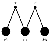
Figure 11:

In a similar way as in Claim 5.9, we can show that, for any neighbor $y$ of $x$ in the quasi-clique $Q_{\mathfrak{h}}(F_{2})$ and for any fat vertex $F\in V^{f}_{\mathfrak{h}}(y)$, it follows that $|N^{s}_{\mathfrak{h}}(F_{1},F)|\leq 1$. Observing that $y$ has only one fat neighbor besides the fat vertex $F_{2}$, this implies that $y$ has at most one neighbor in $Q_{\mathfrak{h}}(F_{1})$ besides $x$. Suppose that $a_{1}=|V(Q_{\mathfrak{h}}(F_{1}))|,\leavevmode\nobreak\ a_{2}=|V(Q_{\mathfrak{h}}(F_{2}))|$. Since $x^{\prime}$ has no neighbor in the quasi-clique $Q_{\mathfrak{h}}(F_{1})$, it implies that $Q_{\mathfrak{h}}(F_{1})$ cannot be a clique by Lemma 5.5. Therefore, the subgraph of $G$ induced by $V(Q_{\mathfrak{h}}(F_{1}))-\{x\}$ is not a clique. By counting the number of triangles throught $x$ we obtain

$$\begin{split}A_{(x,x)}^{3}&\leq 2\left(\binom{a_{1}-1}{2}-1\right)+2\binom{a_{2}-2}{2}+2(a_{2}-2)\\ &\leq 2\left(\binom{2t+1}{2}-1\right)+2\binom{2t}{2}+2\cdot 2t\\ &=8t^{2}+4t-2.\end{split}$$

But, as $G$ has the same spectrum as the $2$-clique extension of the $(t+1)\times(t+1)$-grid, we obtain that $A_{(x,x)}^{3}=8t^{2}+4t$ by (6). This gives a contradiction. Hence, we just showed that all the vertices of $G$ are of Type $2$.

Now, consider the following equivalence relation $\mathcal{R}$ on the vertex set $V(G)$:

$$x\mathcal{R}x^{\prime}{\text{ if and only if }}\{x\}\cup N(x)=\{x^{\prime}\}\cup N(x^{\prime}),{\text{ where }}x,x^{\prime}\in V(G).$$

It means that for each vertex $x$, there exists an unique distinct vertex $x^{\prime}$ such that $x\mathcal{R}x^{\prime}$ and $x^{\prime}\sim x$. So two vertices in the same equivalent class induce a $2$-clique. Let us define a graph $\underline{G}$ whose vertices are the equivalent classes, and such that two classes $\{x,x^{\prime}\}$ and $\{y,y^{\prime}\}$ are adjacent in $\underline{G}$ if and only if $x\sim y,x^{\prime}\sim y,x\sim y^{\prime},x^{\prime}\sim y^{\prime}.$ Then $\underline{G}$ is a regular graph with valency $2t$, and $G$ is the $2$-clique extension of $\underline{G}$. Note that the spectrum of $\underline{G}$ follows immediately from (1) and (2) and is equal to

$$\big{\{}(2t)^{1},(t-1)^{2t},(-2)^{t^{2}}\big{\}}.$$

Since $\underline{G}$ is a connected regular graph with valency $2t$ with multiplicity $1$, and since it has exactly three distinct eigenvalues, it follows that $\underline{G}$ is a strongly regular graph with parameters $\big{(}(t+1)^{2},2t,t-1,2\big{)}$. From [15], it follows that if $t\neq 3$, then the graph with these parameters is unique and is the $(t+1)\times(t+1)$-grid. So we obtained that $G$ is the $2$-clique extension of the $(t+1)\times(t+1)$-grid when $t>4$. ∎

Now let us assume that we are in Case 2, that is $q_{2t}=0,\leavevmode\nobreak\ q_{2t+1}=2t+2$, and $q_{2t+2}=1$. We have already seen that $n_{4}=0$. We will show that this case is impossible. But to show this, we will need a few lemmas.

As a vertex of Type $1$ or Type $2$ lies in two distinct quasi-cliques of order $2t+2$ and $q_{2t+2}=1$, we find that there are no vertices of Type $1$ or Type $2$. So we obtain $n_{1}=n_{2}=0$. This implies $n_{3}=2t+2$ and $n_{5}=2t(t+1)$ by (29) and (30). As $n_{1}=0$, all quasi-cliques are actually cliques since every vertex is adjacent to all of the vertices in the same quasi-clique except itself.

Let $Q$ be the unique quasi-clique of order $2t+2$ and let $\mathcal{L}=\{Q^{\prime}\mid Q^{\prime}$ is a quasi-clique of order $2t+1\}$. We already noticed that $Q$ and $Q^{\prime}\in\mathcal{L}$ are actually cliques. Now we will show the following lemma:

Lemma 6.2.

For every vertex $x$ in $Q$, there exists an unique quasi-clique $Q^{\prime}_{x}\in\mathcal{L}$ such that $x\in V(Q^{\prime}_{x})$;

For distinct vertices $x_{1}$ and $x_{2}$ in $Q$, the quasi-cliques $Q^{\prime}_{x_{1}}$ and $Q^{\prime}_{x_{2}}$ are distinct;

For every quasi-clique $Q^{\prime}\in\mathcal{L}$, there exists an unique vertex $x_{Q^{\prime}}$ such that $x_{Q^{\prime}}\in V(Q)$;

For distinct quasi-cliques $Q_{1}^{\prime}$ and $Q_{2}^{\prime}$ in $\mathcal{L}$, the vertices $x_{Q_{1}^{\prime}}$ and $x_{Q_{2}^{\prime}}$ are distinct.

Proof.

$(i)$ It follows from before the fact that, for all $x\in V(Q)$, $x$ is of Type $3$.

$(ii)$ By Lemma 3.3 $(ii)$, we have $|V(Q^{\prime})\bigcap V(Q)|\leq 1$ for any $Q^{\prime}\in\mathcal{L}$. If $Q^{\prime}_{x_{1}}$ and $Q^{\prime}_{x_{2}}$ are the same, then $Q^{\prime}_{x_{1}}$ shares two common vertices with $Q$, it is not possible. So the result follows.

$(iii)$ Since $|\mathcal{L}|=q_{2t+1}=2t+2$ and $|V(Q)|=2t+2$, it follows from $(i)$ and $(ii)$.

$(iv)$ It follows from $(i)$-$(iii)$. ∎

Let $W=V(G)-V(Q)$ and let $G^{\prime}$ be the induced subgraph of $G$ on $W$. Let $G^{\prime\prime}$ be the spanning subgraph of $G^{\prime}$ such that the vertices $w_{1},\leavevmode\nobreak\ w_{2}$ are adjacent in $G^{\prime\prime}$ if there exists a quasi-clique $Q^{\prime}\in\mathcal{L}$ such that $w_{1}$ and $w_{2}$ are in $Q^{\prime}$. Now we have the following lemma:

Lemma 6.3.

The graph $G^{\prime\prime}$ is the line graph of the cocktail-party graph $CP(2t+2)$.

Proof.

Define the graph $H$ with vertex set $\mathcal{L}$ and two quasi-clique $Q_{1}^{\prime},Q_{2}^{\prime}\in\mathcal{L}$ are adjacent if they intersect in a unique element. It is easy to see that the graph $G^{\prime\prime}$ is the line graph of $H$. As any quasi-clique $Q^{\prime}$ of $\mathcal{L}$ has $2t$ vertices in $W$ and any vertex in $W$ lies in two quasi-cliques in $\mathcal{L}$, it follows that $H$ is $2t$-regular. So $H$ is the cocktail-party graph $CP(2t+2)$ as it has $2t+2$ vertices. Hence, the lemma holds. ∎

Let $\Omega=\{x_{1},\ldots,x_{t+1},x_{1}^{\prime},x_{2}^{\prime},\ldots,x_{t+1}^{\prime}\}$, and let $\Omega^{2}=\{2\text{-subsets of }\Omega\}-\bigcup_{i=1}^{t+1}\{x_{i},x_{i}^{\prime}\}$. (For convenience, we will use $x_{i}x_{j}$ to represent the subset $\{x_{i},x_{j}\}$, and similarly for the other $2$-subsets in $\Omega^{2}$.) We define the graph $G^{0}$ with vertex set $\Omega\bigcup\Omega^{2}$ and three kinds of edges as follows:

1. the edges of the form $\{x,y\}$, where $x,y\in\Omega$;

2. the edges of the form $\{x,xy\}$, where $x\in\Omega,xy\in\Omega^{2}$;

3. the edges of the form $\{xy,xz\}$, where $xy,xz\in\Omega^{2}$.

By Lemma 6.3, Lemma 6.2 and the definition of $Q$, we see that $G^{0}$ is isomorphic to a spanning subgraph of $G$, and hence we can identify $V(G)$ with $\Omega\bigcup\Omega^{2}$.

Now consider the partition $\pi=\{V_{1},V_{2},V_{3},V_{4}\}$ of $V(G)$, where

$$V_{1}=\{x_{1},x_{1}^{\prime}\},$$

$$V_{2}=\{x_{i},x_{i}^{\prime}:2\leq i\leq t+1\},$$

$$V_{3}=\{x_{1}x_{i},x_{1}x_{i}^{\prime},x_{1}^{\prime}x_{i},x_{1}^{\prime}x_{i}^{\prime}:2\leq i\leq t+1\},$$

$$V_{4}=\{x_{i}x_{j},x_{i}x_{j}^{\prime},x_{i}^{\prime}x_{j},x_{i}^{\prime}x_{j}^{\prime},2\leq i<j\leq t+1\}.$$

The quotient matrix $\widetilde{B}$ of the adjacency matrix $A$ of $G$ with respect to the above partition $\pi$ is given as follows:

$$\widetilde{B}=\left(\begin{array}[]{cccc}1&2t&2t&0\\ 2&2t-1&2&2t-2\\ 1&1&\alpha&4t-1-\alpha\\ 0&2&\frac{2(4t-1-\alpha)}{t-1}&4t-1-\frac{2(4t-1-\alpha)}{t-1}\end{array}\right)$$ (38)

with $2t\leq\alpha\leq 2t+1$.

We will show that $\alpha=2t+1$, and hence the partition $\pi$ is an equitable partition of $G$.

To show this, note that by (6), we have

$$\begin{split}A_{(x_{1},x_{1}^{\prime})}^{3}&=24t+1-(5-2t)\lambda_{x_{1},x_{1}^{\prime}}\\ &=24t+1-(5-2t)\cdot 2t\\ &=4t^{2}+14t+1.\end{split}$$ (39)

On the other hand,

$$A_{(x_{1},x_{1}^{\prime})}^{3}=4t+1+\sum\nolimits_{z\in G_{1}(x_{1})\bigcap G_{1}(x_{1}^{\prime})}\lambda_{x_{1},z}+\sum\nolimits_{z\in G_{2}(x_{1})\bigcap G_{1}(x_{1}^{\prime})}\mu_{x_{1},z},$$ (40)

where $|G_{1}(x_{1})\bigcap G_{1}(x_{1}^{\prime})|=2t,\leavevmode\nobreak\ |G_{2}(x_{1})\bigcap G_{1}(x_{1}^{\prime})|=2t$ and

$$\begin{split}\lambda_{x_{1},z}=2t+1,&\text{ for }z\in G_{1}(x_{1})\bigcap G_{1}(x_{1}^{\prime}),\\ 3\leq\mu_{x_{1},z}\leq 4,&\text{ for }z\in G_{2}(x_{1})\bigcap G_{1}(x_{1}^{\prime}).\end{split}$$

Then, from (39) and (40), we obtain that

$$\mu_{x_{1},z}=4,\text{for }z\in G_{2}(x_{1})\bigcap G_{1}(x_{1}^{\prime}),$$

which implies that $\alpha=2t+1$. Therefore, we have an equitable partition with partition diagram as shown in Figure 12.

Figure 12: Equitable partition

In this case, the quotient matrix (38) becomes

$$\widetilde{B}=\left(\begin{array}[]{cccc}1&2t&2t&0\\ 2&2t-1&2&2t-2\\ 1&1&2t+1&2t-2\\ 0&2&4&4t-5\end{array}\right)$$ (41)

with eigenvalues $\big{\{}4t+1,2t-1,t-2\pm\sqrt{t^{2}-1}\big{\}}$.

From Lemma 2.3, we find that the eigenvalues of $\widetilde{B}$ should be the eigenvalues of $A$. But $B$ has eigenvalues $t-2\pm\sqrt{t^{2}-1}$, which are not the eigenvalues of $A$. So we obtain a contradiction. This shows that the case $q_{2t}=0,\leavevmode\nobreak\ q_{2t+1}=2t+2,\leavevmode\nobreak\ q_{2t+2}=1$ is not possible. This concludes the proof to show that $G$ is the $2$-clique extension of the $(t+1)\times(t+1)$ grid.

Remark 6.4.

Note that we used walk-regularity (which follows from the fact that the $2$-clique extension of the $(t+1)\times(t+1)$-grid is regular with exactly $4$ distinct eigenvalues) to show this result, and therefore it is not so clear how to extend this result to the $2$-clique extension of a non-square grid graph.

References

- [1] A. Abiad, A.E. Brouwer, and W.H. Haemers, Godsil-McKay switching and isomorphism, Electr. J. Linear Algebra 28 (2015), 4–11.
- [2] S. Bang, E.R. van Dam, and J.H. Koolen, Spectral characterization of the Hamming graphs, Linear Algebra Appl. 429 (2008), 2678–2686.
- [3] A.E. Brouwer, A.M. Cohen, and A. Neumaier, Distance-Regular Graphs, Springer-Verlag, Berlin-New York, 1989.
- [4] E.R. van Dam, Regular graphs with four eigenvalues, Linear Algebra Appl. 226-228 (1995), 139–162.
- [5] E.R. van Dam, Graphs with Few Eigenvalues - an Interplay between Combinatorics and Algebra, Ph.D. thesis, 1996.
- [6] E.R. van Dam and W.H. Haemers, Which graphs are determined by their spectrum?, Linear Algebra Appl. 373 (2003), 241–272.
- [7] E.R. van Dam, J.H. Koolen, and H. Tanaka, Distance-regular graphs, Electron. J. Combin. (2016), DS22.
- [8] A. Gavriliouk and J.H. Koolen, On a characterization of the Grassmann graphs over the binary field, preprint (2016).
- [9] C. Godsil and G. Royle, Algebraic Graph Theory, Springer-Verlag, New York, 2001.
- [10] G. Greaves, J. Koolen, A. Munemasa, Y. Sano, and T. Taniguchi, Edge-signed graphs with smallest eigenvalue greater than , J. Combin. Theory Ser. B 110 (2015), 90–111.
- [11] W.H. Haemers, Interlacing eigenvalues and graphs, Linear Algebra Appl. 226-228 (1995), 593–616.
- [12] A.J. Hoffman, On the polynomial of a graph, Amer. Math. Monthly 70 (1963), 30–36.
- [13] H.J. Jang, J. Koolen, A. Munemasa, and T. Taniguchi, On fat Hoffman graphs with smallest eigenvalue at least -3, ARS Mathematica Contemporanea 7 (2014), 105–121.
- [14] J.H. Koolen, J.Y. Yang and Q.Q. Yang, A generalization of a theorem of Hoffman, submitted.
- [15] S.S. Shrikhande, The uniqueness of the association scheme, Ann. Math. Statist. 30 (1959), 781–798.
- [16] R. Woo and A. Neumaier, On graphs whose smallest eigenvalue is at least , Linear Algebra Appl. 226-228 (1995), 577–591.
- [17] H. Yu, On the limit points of the smallest eigenvalues of regular graphs, Des. Codes Cryptography 65 (2012), 77–88.