QoS constrained Large Scale Web Service Composition using Abstraction Refinement

Abstract

Efficient service composition in real time, while satisfying desirable Quality of Service (QoS) guarantees for the composite solution has always been one of the topmost research challenges in the domain of service computing. On one hand, optimal QoS aware service composition algorithms, that come with the promise of solution optimality, are inherently compute intensive, and therefore, often fail to generate the optimal solution in real time for large scale web services. On the other hand, heuristic solutions that have the ability to generate solutions fast and handle large and complex service spaces, settle for sub-optimal solution quality. The problem of balancing the trade-off between compute efficiency and optimality in service composition has alluded researchers for several decades, and several proposals for taming the scale and complexity of web service composition have been proposed in literature. In this paper, we present a new perspective towards this trade-off in service composition based on abstraction refinement, that can be seamlessly integrated on top of any off-the-shelf service composition method to tackle the space complexity, thereby, making it more time and space efficient. Instead of considering services individually during composition, we propose a set of abstractions and corresponding refinements to form service groups based on functional characteristics. The composition and QoS satisfying solution construction steps are carried out in the abstract service space. Our abstraction refinement methods give a significant speed-up compared to traditional composition techniques, since we end up exploring a substantially smaller space on average. Experimental results on benchmarks show the efficiency of our proposed mechanism in terms of time and the number of services considered for building the QoS satisfying composite solution.

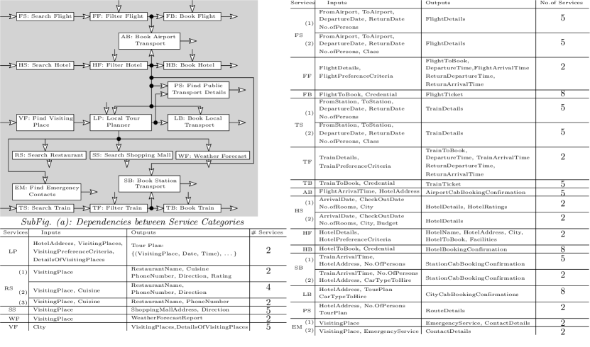
Figure 1: Service repository

1 Introduction

In recent times, web services have become the most powerful gateway to massive repositories of information and applications to serve user queries. A web service is a software component that performs a specific task and is characterized by its functional attributes (inputs / outputs) and non functional Quality of Service (QoS) attributes like response time, throughput, reliability, availability, compliances etc. In many cases, it is not possible to serve a user specified query with a single web service, for which, composition is required to invoke multiple web services in a specific order. During service composition, on one side, it is important to ensure that functional dependencies are met, i.e., the input-output dependencies of the services are honored. On the other hand, it is also important to ensure the overall non functional requirements, i.e., overall QoS values of the solution [1] and satisfy constraints on them as applicable. Scalability of composition algorithms for real time query response has always been a major element of concern [2, 3]. With tremendous increase in the scale of web services [4], large scale web service composition [5] is becoming an increasingly important challenge.

A large body of literature in service composition deals with methods for computing the optimal composition [6, 7, 8] satisfying QoS constraints as applicable. These methods, though having the promise of optimality of the composite solution, often fail to scale to large web service repositories for real time response at query time. Service composition approaches based on A*[9], constraint satisfiability[10] and graph search[11, 12], fail to deliver the expected performance, due to the inherent complexities of the methods they use to navigate and search for the optimal solution in the composed state space. Comparable advances have also been made in the area of heuristic approaches towards service composition [11], wherein, the solution optimality is compromised to make the solution generation fast, scalable and efficient at query time. Indeed, balancing the trade-off between optimality and efficiency has always been a foremost research challenge with several widely varying proposals [13, 14, 15] in literature.

In this work, we examine the problem of QoS constrained query time service composition from a completely different perspective, and propose a technique that can be seamlessly integrated on top of any off-the-shelf service composition method to tackle the space complexity, thereby, making it more time and space efficient. Our technique is based on the idea of abstraction refinement [39], which was originally developed for handling large state spaces in the context of formal verification. Our proposal has two major steps. As a first step, we aim to expedite the solution computation time of the underlying service composition method. Instead of considering services individually during composition, we propose a set of abstractions and corresponding refinements to form service groups based on functional characteristics and the composition is carried out in the abstract service space. Our approach has the guarantee of always being able to generate a QoS satisfying solution, if one exists. Abstraction reduces the search space significantly, and thus speeds up the composition and solution generation steps. While this can expedite the solution construction step to a great extent, this also entails a possibility that it may fail to generate any solution satisfying a given set of QoS constraints, though the individual services allow a valid solution. Therefore, as a second step, we propose to refine an abstraction to generate the composite solution with desired QoS values. A QoS satisfying solution, if one exists, can be constructed from the abstraction with refinement. In the worst case (which is rare in our experiments), our approach may end up exploring the complete composition graph constructed on individual services, and thereby never miss a solution if one exists. In general, a solution satisfying all the QoS constraints can be obtained efficiently from the abstract graph. Abstraction is done at preprocessing / design time, whereas, the composition is done at query time. Though the abstraction step does not affect run-time composition performance, the refinement step (if needed), being done at query time, does add up a non-negligible overhead to the composition process. However, as can be seen from our experiments, the underlying service composition method is still much faster in the average case, when compared with its performance without the abstraction and refinement steps.

We perform extensive experiments on the popular benchmarks ICEBE-2005 [16] and WSC-2009 [18] to demonstrate the power of abstraction. In each case, as evident from the experiments detailed in Section 4, our method adds orders of magnitude scalability, when considered on top of three recent [19, 12, 9] service composition methods.

2 Motivating Example

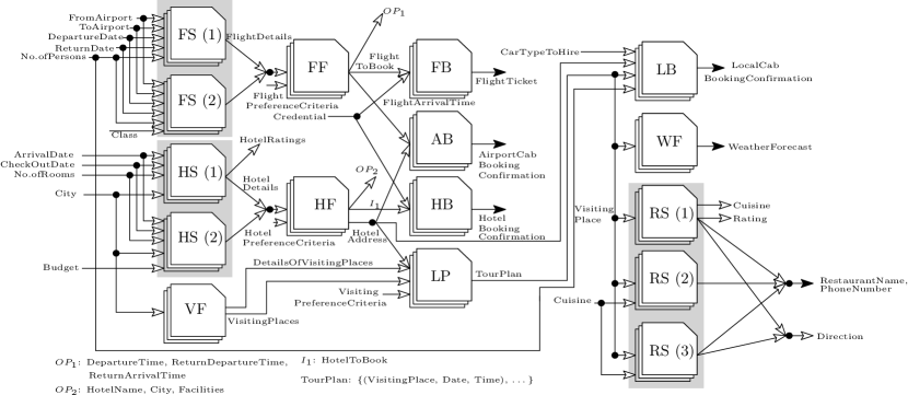
Figure 2: Service dependency graph to serve ${\cal{Q}}$

We use an example description of a service repository for tour planning, to illustrate our methods throughout the paper. The service repository contains 99 services. The services are broadly classified into 19 different service categories depending on the specific task each service caters to, as shown in Figure 1. SubFigure (a) of Figure 1 shows the dependencies between the service categories. Each rectangular box of the subFigure represents a service category and a directed edge between two service categories represents an input-output dependency, i.e. some / all outputs generated by the source task go as inputs into the destination task. The input-output sets of the services for each category are shown in the $2^{nd}$ and the $3^{rd}$ columns of the table of Figure 1. For a specific category, there are multiple services which are able to fulfill the service task, and these are shown as sub-categories in the $1^{st}$ column. The input-output set of two services in a service category can be different, in which case they are placed in an appropriate sub-category. Consider the flight search (FS) service category consisting of 10 services. As shown in Figure 1, there are two sub-categories, $FS^{(1)}$ and $FS^{(2)}$, differing in their input sets. Out of the 10 services for $FS$, 5 services have the same input set and are in sub-category $FS^{(1)}$, whereas, the other 5 services have a different input set and are in sub-category $FS^{(2)}$. The outputs of both the sub-categories are same in this case. A similar clustering based on both inputs and outputs can be seen for the service task $EM$. It may be noted that services in the same category / sub-category may have different QoS values. For the sake of simplicity, we consider here only two QoS parameters, namely, the response time and invocation cost. Each service, therefore, is associated with values of these two parameters.

Consider a query ${\cal{Q}}$ with inputs {FromAirport, ToAirport, DepartureDate, ReturnDate, No.ofPersons, Class, FlightPreferenceCriteria, Credential, ArrivalDate, CheckOutDate, No.ofRooms, City, Budget, HotelPreferenceCriteria, VisitingPreferenceCriteria, Cuisine} and desired output {FlightTicket, HotelBookingConfirmation, AirportCabBookingConfirmation, CityCabBookingConfirmations, WeatherForecastReport, RestaurantName, PhoneNumber}. Consider constraints on maximum response time and invocation cost for the composite service as 1 second and $10 respectively. The objective is to serve ${\cal{Q}}$, while satisfying the QoS constraints.

In classical service composition methods, the input-output functional service dependencies are represented by a directed graph, usually referred to as the functional dependency graph [19]. The composition solution corresponding to a service query is either a path or a subgraph of the dependency graph, depending on the functional parameter [19] and the nature of the services being composed [20]. The size of the dependency graph depends on the number of services in the service repository and their inputs and outputs. A service repository may contain a large number of web services. In this case, construction of the dependency graph incurs a lot of time and space. Considering the above example, the functional dependency graph for serving ${\cal{Q}}$ involving 64 services is shown in Figure 2. Each block in Figure 2 represents multiple services having identical set of inputs and outputs.

Managing the complexity of the dependency graph and the solution extraction step thereafter, has been the foremost challenge for composition. Optimal service composition methods based on ILP [6] or sub-optimal heuristics [14] both have their own limitations in handling such graphs at the web scale, since they traverse the concrete service space to generate a solution. While optimal methods encode the entire dependency graph as a set of constraints, heuristics employ smart traversal mechanisms to tame the space complexity. Our perspective in contrast is to work with any of these methods but on a reduced abstract space, created from the concrete service repository, and refined at query time. We show through our experiments that the composition and QoS constraint satisfying solution construction steps are more efficient when considered on the abstracted reduced search space using any of the methods discussed above. In this paper, we propose several such abstractions that can expedite any composition method to a significant extent.

3 Detailed Methodology

The service composition problem considered here is same as in classical services work [1]. The inputs to the problem are:

• A set of web services $S=\{{\cal{S}}_{1},{\cal{S}}_{2},\ldots,{\cal{S}}_{n}\}$

• For each web service ${\cal{S}}_{i}\in S$, a set of inputs ${\cal{S}}_{i}^{ip}$ and a set of outputs ${\cal{S}}_{i}^{op}$

• For each web service ${\cal{S}}_{i}\in S$, a set of QoS parameters (e.g., Response time, Reliability, Invocation cost etc) represented as a tuple

• A set of concepts [21] (optional) that capture information about semantically equivalent service descriptions

• A query ${\cal{Q}}$, specified by a set of inputs ${\cal{Q}}^{ip}$ and a set of requested outputs ${\cal{Q}}^{op}$

• An optional set $\cal{C}$ of QoS constraints represented by a tuple on the composite solution providing bounds on the worst case values

The objective of classical QoS constrained service composition is to serve ${\cal{Q}}$ by suitable composition of the services in $\{{\cal{S}}_{1},\ldots,{\cal{S}}_{n}\}$ preserving functional dependencies and satisfying all QoS constraints. The complexity of finding a QoS satisfying optimal solution depends on the QoS parameter under consideration. On one hand, for QoS parameters like response time and throughput, the complexity is polynomial in the number of services [22]. On the other hand, for QoS parameters like reliability, availability, reputation, invocation cost, the problem is NP-hard [22].

As discussed earlier, our motivation in this work is to create a framework that can seamlessly fit on top of any service composition approach and expedite its performance. In the following discussion, we explain how our abstraction methods leverage on the functional characteristics of the services. Abstractions are done in a preprocessing phase, before composition and query arrival. In this paper, we consider four levels of abstraction. In each level, one or multiple services are abstracted by a new service. The main objective of abstraction is to reduce the number of services to be considered for query processing during composition.

3.1 Abstraction of equivalent services

Before we discuss the details of the abstraction, we begin with a few definitions.

Definition 3.1.

[Input (Output) Equivalence:] Two services ${\cal{S}}_{1},{\cal{S}}_{2}$ are input (output) equivalent, expressed as ${\cal{S}}_{1}\simeq_{i}{\cal{S}}_{2}$ (${\cal{S}}_{1}\simeq_{o}{\cal{S}}_{2}$) if their input (output) sets are identical. $\blacksquare$

We now illustrate the notion of a concept and how it helps in finding identical inputs and outputs between services, even when the names do not match exactly. An input (output) $i_{1}$ ($o_{1}$) of a service ${\cal{S}}_{1}$ is said to be identical to an input (output) $i_{2}$ ($o_{2}$) of a service ${\cal{S}}_{2}$, if both of them semantically refer to the same concept. Consider two flight search services ${\cal{S}}_{1}$ and ${\cal{S}}_{2}$. The input set of ${\cal{S}}_{1}$ is {from, to, departureDate, noOfPersons} and the input set of ${\cal{S}}_{2}$ is {fromAirport, toAirport, departureDate, noOfPersons}. The inputs of ${\cal{S}}_{1}$ and ${\cal{S}}_{2}$ are considered identical since both of them refer to the same concept, i.e., departure airport and arrival airport respectively. A set of such concepts capture additional semantic information between service descriptions and accompany any service repository [21].

We now present a few results that help us to build the foundations of our abstraction and the guarantees they offer. All proofs are available in the appendix.

Lemma 1.

The binary relation $``\simeq_{i}"$ defined over a set of services is an equivalence relation. $\blacksquare$

On similar lines, $``\simeq_{o}"$ is an equivalence relation as well.

Definition 3.2.

[Equivalent Services:] Two services ${\cal{S}}_{1},{\cal{S}}_{2}$ are equivalent (${\cal{S}}_{1}\simeq{\cal{S}}_{2}$), if they are input equivalent, ${\cal{S}}_{1}\simeq_{i}{\cal{S}}_{2}$, as well as output equivalent, ${\cal{S}}_{1}\simeq_{o}{\cal{S}}_{2}$. $\blacksquare$

The following holds with a similar reasoning.

Lemma 2.

The binary relation $``\simeq"$ defined over a set of services is an equivalence relation. $\blacksquare$

The notion of equivalence is purely syntactic, in other words, two equivalent services can have different QoS parameter values. In the first level of abstraction, we abstract equivalent services by a new service. The services in the service repository are divided into equivalence classes ($``\simeq"$ is an equivalence relation). The set of all equivalence classes of $S$ forms a partition of $S$. Every service of $S$ thus belongs to one and only one equivalence class. Each equivalence class is then represented by an abstract service. This reduces the number of services in the dependency graph considered at query time. Therefore, computing the solution to a query becomes easier. Evidently, the QoS values of the composite solution may be affected as a result of this abstraction step.

Each equivalence class of services $\{{\cal{S}}_{i1},{\cal{S}}_{i2},\ldots,{\cal{S}}_{ik}\}\subseteq S$ is abstracted by a new representative service ${\cal{S}}^{(1)}_{i}$. The inputs and outputs of ${\cal{S}}^{(1)}_{i}$ are same as ${\cal{S}}_{ij}$. Consider $S^{(1)}=\{{\cal{S}}^{(1)}_{1},{\cal{S}}^{(1)}_{2},\ldots,{\cal{S}}^{(1)}_{n_{1}}\}$ be the set of $n_{1}$ abstract services generated from the original set of $n$ services. Evidently, the set of services corresponding to ${\cal{S}}^{(1)}_{i}$ and ${\cal{S}}^{(1)}_{j}$ are mutually exclusive for $i\neq j$. Therefore, the following holds.

Lemma 3.

The number of services after the first level of abstraction is less than or equal to the total number of services in the service repository, i.e., $n_{1}\leq n$. $\blacksquare$

Algorithm 1 details the abstraction procedure. Step 6 is the key step of Algorithm 1. In this step, for each service ${\cal{S}}_{i}\in S$, all other services in the repository are examined to identify whether they are equivalent to ${\cal{S}}_{i}$. The complexity of this step is $O(n)$ and thereby, the overall complexity of the algorithm is $O(n^{2})$, where $n$ is the number of services in the original service repository.

Algorithm 1 Abstraction of Equivalent Services

1:Input: $S=\{{\cal{S}}_{1},{\cal{S}}_{2},\ldots,{\cal{S}}_{n}\}$

2:Output: Abstract Service set $S^{(1)}=\{{\cal{S}}^{(1)}_{1},{\cal{S}}^{(1)}_{2},\ldots,{\cal{S}}^{(1)}_{n_{1}}\}$

3:$S^{\prime}=S$;

4:repeat

5:    Remove an arbitrary service ${\cal{S}}_{i}$ from $S^{\prime}$;

6:    ${\cal{U}}$ = services equivalent to ${\cal{S}}_{i}$;

7:    Construct a service ${\cal{S}}^{(1)}_{i}$ corresponding to ${\cal{U}}\cup\{{\cal{S}}_{i}\}$;

8:    Inputs of ${\cal{S}}^{(1)}_{i}$ = inputs of ${\cal{S}}_{i}$;

9:    Outputs of ${\cal{S}}^{(1)}_{i}$ = outputs of ${\cal{S}}_{i}$;

10:    Add ${\cal{S}}^{(1)}_{i}$ to $S^{(1)}$;

11:    $S^{\prime}\leftarrow S^{\prime}\smallsetminus({\cal{U}}\cup\{{\cal{S}}_{i}\})$; $\triangleright$ $``\smallsetminus"$ represents set minus operator

12:until $S^{\prime}$ is not empty

Example 3.1.

We now illustrate the effect of this abstraction step on our motivating example discussed in Section 2. The services in a sub-category have identical set of inputs and outputs and therefore, they are equivalent. Hence, each sub-category, consisting of multiple services, is abstracted by a new service. The service repository contains 26 sub-categories in total. Therefore, the number of services after this abstraction step is reduced from 99 to 26. Each block in Figure 2, represents a single abstract service instead of multiple services. $\blacksquare$

The crux of this abstraction is to merge equivalent services based on input-output equivalence. The challenge now is to assign a representative QoS value to the created abstract service, since services inside an equivalence class may have widely different QoS values. For this, we choose for each class, the best representative service $s$ (defined formally below) and assign the QoS values of $s$ to the abstract service. The choice of $s$ for each class is done as explained below.

Consider an abstract service ${\cal{S}}^{(1)}_{i}\in S^{(1)}$ corresponding to an equivalence class ${\hat{S}}_{(i)}=\{{\cal{S}}_{i1}$, ${\cal{S}}_{i2}$, $\ldots,{\cal{S}}_{ik}\}$. If there exists any service ${\cal{S}}_{ij}\in{\hat{S}}_{(i)}$, such that, it has the best values for all the QoS parameters among all the services in ${\hat{S}}_{(i)}$, we assign the values of all QoS parameters of ${\cal{S}}_{ij}$ to ${\cal{S}}^{(1)}_{i}$. Otherwise, we choose the best representative one in terms of the QoS parameter values. Since the QoS parameters are disparate in nature, we first normalize their values for each service in an equivalence class. QoS parameters (QP) like reliability and availability, for which a high value is desirable (i.e., positively monotonic), are normalized as:

$$NV({\cal{S}}_{ij}(QP))=\begin{cases}1\text{\indent\indent\indent\indent~{}~{}~{}, if }Max(QP)=Min(QP)\\ \frac{{\cal{S}}_{ij}(QP)-Min(QP)}{Max(QP)-Min(QP)}\text{, otherwise }\end{cases}$$ (1)

where ${\cal{S}}_{ij}(QP)$ is the value of QP for service ${\cal{S}}_{ij}\in\{{\cal{S}}_{i1}$, ${\cal{S}}_{i2}$, $\ldots,{\cal{S}}_{ik}\}$, $Max(QP)$ and $Min(QP)$ are the maximum and minimum values of QP across the set ${\cal{S}}_{i1}$, ${\cal{S}}_{i2}$, $\ldots,{\cal{S}}_{ik}$ respectively. Similarly, for QoS parameters like response time, invocation cost, total number of invocations for which a low value is desirable (i.e., negatively monotonic), the normalization is defined as:

$$NV({\cal{S}}_{ij}(QP))=\begin{cases}1\text{\indent\indent\indent\indent~{}~{}~{}, if }Max(QP)=Min(QP)\\ \frac{Max(QP)-{\cal{S}}_{ij}(QP)}{Max(QP)-Min(QP)}\text{, otherwise }\end{cases}$$ (2)

The normalized value (NV) of each QoS parameter (QP) is positively monotonic and lies between 0 to 1. Once we normalize the QoS parameters, we compute the deviation of the QoS parameter of a service from the best value of the QoS parameter as follows:

$$Deviation({\cal{S}}_{ij}(QP))=1-NV({\cal{S}}_{ij}(QP))$$ (3)

We now define the notion of the best representative service.

Definition 3.3.

[Best Representative Service:] The best representative service of an equivalence class is a service for which the maximum deviation across all QoS parameters is minimum among all services in that class. $\blacksquare$

If multiple services exist for which the maximum deviation is minimum, we resolve the tie by considering the second maximum deviation for each service across all parameters and selecting the service for which the second maximum deviation is minimum among the tied services. We continue the procedure until the tie is resolved. Once we select the best representative service $s$, we assign all the values of its QoS parameters to ${\cal{S}}^{(1)}_{i}$. Algorithm 2 presents the formal algorithm. We illustrate our method on the example below.

Example 3.2.

Consider two input-output equivalent services ${\cal{S}}_{1}$ and ${\cal{S}}_{2}$ and two QoS parameters, namely, invocation cost and reliability. The QoS values of ${\cal{S}}_{1}$ and ${\cal{S}}_{2}$ are (100, 0.96) and (150, 0.98) respectively. By our abstraction mechanism, ${\cal{S}}_{1},{\cal{S}}_{2}$ are abstracted by a new service ${\cal{S}}^{(1)}_{1}$. To assign the value of the QoS parameters of ${\cal{S}}^{(1)}_{1}$, we compute the $NV$ values as follows. $NV({\cal{S}}_{1}(InvocationCost))=1$, $NV({\cal{S}}_{1}(Reliability))=0.43$, $NV({\cal{S}}_{2}(InvocationCost))=0.83$, $NV({\cal{S}}_{2}(Reliability))=0.71$. Consider the maximum and minimum values of invocation cost among all services are 400 and 100 respectively and the same for reliability are 0.99 and 0.93 respectively. The maximum deviation for ${\cal{S}}_{1}$ across the two QoS parameters is $Max((1-1),(1-0.43))=0.57$, the same for ${\cal{S}}_{2}$ is $Max((1-0.83),(1-0.71))=0.29$. We select ${\cal{S}}_{2}$ and assign the values of the QoS parameters of ${\cal{S}}_{2}$ to ${\cal{S}}^{(1)}_{1}$, since for ${\cal{S}}_{2}$, the maximum deviation across all parameters is minimum. $\blacksquare$

Algorithm 2 Identify representative service

1:Input: ${\hat{S}}_{(i)}=\{{\cal{S}}_{i1}$, ${\cal{S}}_{i2}$, $\ldots,{\cal{S}}_{ik}\}$$\triangleright$ Set of equivalent services

2:Output: ${\cal{S}}_{il}\in{\hat{S}}_{(i)}$$\triangleright$ Chosen service for QoS assignment

3:for ${\cal{S}}_{ij}\in{\hat{S}}_{(i)}$ do

4:    for each $QP\in$ Set of QoS parameters do

5:       Compute $NV({\cal{S}}_{ij}(QP))$;

6:       Compute $Deviation({\cal{S}}_{ij}(QP))=1-NV({\cal{S}}_{ij}(QP))$;

7:    end for

8:    $\delta({\cal{S}}_{ij})\leftarrow MAX_{QP\in\text{Set of QoS parameters}}$ ($Deviation({\cal{S}}_{ij}(QP))$);

9:end for

10:Identify the service ${\cal{S}}_{il}\in{\hat{S}}_{(i)}$, such that $\delta({\cal{S}}_{il})=Min_{{\cal{S}}_{ij}\in{\hat{S}}_{(i)}}\delta({\cal{S}}_{ij})$;

11:$\triangleright$ In case of a tie, break the tie as discussed above

We now discuss the correctness and optimality guarantee of our QoS assignment mechanism. Consider a service ${\cal{S}}^{(1)}_{i}\in S^{(1)}$ corresponding to its equivalence class ${\hat{S}}_{(i)}$. The QoS assignment to ${\cal{S}}^{(1)}_{i}$ ensures the following lemma.

Lemma 4.

For a single QoS parameter, the QoS value assigned to ${\cal{S}}^{(1)}_{i}$ is optimal among the set of QoS values in ${\hat{S}}_{(i)}$. $\blacksquare$

Lemma 5.

For multiple QoS parameters, the QoS values assigned to ${\cal{S}}^{(1)}_{i}$ belong to the Pareto-optimal front [23] constructed over all the QoS values corresponding to ${\hat{S}}_{(i)}$. $\blacksquare$

3.1.1 Composition with abstract services

We can now use any service composition method at query time over the abstract service set and construct a composite solution that satisfies all QoS constraints, if one exists. The major advantage of the first abstraction step is its guarantee of solution quality (more importantly, optimality) preservation for a single QoS parameter case. Thus, after this abstraction step, if an optimal method is used for composition on the abstract set of services, we are guaranteed to be able to generate the same optimal solution that would have been generated by the optimal method, had the composition been carried out in the original un-abstracted service space without abstraction. On a similar note, if a heuristic approach is used, it is guaranteed that a solution of the same quality can be generated over the abstract space. The results are formalized in the discussion below.

Corollary 1.

For a single QoS parameter, equivalence abstraction is solution quality preserving. $\blacksquare$

Corollary 1 directly follows from Lemma 4. However, for multiple QoS parameters, such a claim does not hold good. Consider the following example.

Example 3.3.

Consider two equivalence classes $\{{\cal{S}}_{1},{\cal{S}}_{2},{\cal{S}}_{3}\}$ and $\{{\cal{S}}_{4},{\cal{S}}_{5},{\cal{S}}_{6}\}$. Consider each service has three QoS parameters: response time, throughput and invocation cost. The values of the QoS parameters for each service are shown as follows: ${\cal{S}}_{1}:(120,50,10),{\cal{S}}_{2}:(75,75,25),{\cal{S}}_{3}:(125,100,20)$, ${\cal{S}}_{4}:(75,50,20),{\cal{S}}_{5}:(150,50,10),{\cal{S}}_{6}:(175,50,10)$. According to our first abstraction strategy, $\{{\cal{S}}_{1},{\cal{S}}_{2},{\cal{S}}_{3}\}$ is abstracted by ${\cal{S}}^{(1)}_{1}$ and $\{{\cal{S}}_{4},{\cal{S}}_{5},{\cal{S}}_{6}\}$ is abstracted by ${\cal{S}}^{(1)}_{2}$. Following our QoS assignment mechanism, ${\cal{S}}_{3}:(125,100,20)$ is chosen as the best representative for the first equivalence class and thus its QoS values are assigned to ${\cal{S}}^{(1)}_{1}$. Similarly, being the best representative of the second class, the QoS values of ${\cal{S}}_{5}:(150,50,10)$ are assigned to ${\cal{S}}^{(1)}_{2}$. It may be noted, in both the cases, the QoS values of the best representative service belong to the Pareto optimal frontier of their respective equivalence classes. Let us now assume ${\cal{S}}^{(1)}_{1}$ and ${\cal{S}}^{(1)}_{2}$ can be composed sequentially. The QoS values of the composite service ${\cal{CS}}:{\cal{S}}^{(1)}_{1}$ followed by ${\cal{S}}^{(1)}_{2}$ are $(275,50,30)$. However, the QoS values of ${\cal{CS}}$ in the composition space of original services do not belong to the Pareto optimal solution frontier, since, the sequential composition of ${\cal{S}}_{1}$ and ${\cal{S}}_{5}$, having QoS values as $(270,50,20)$, dominates ${\cal{CS}}:(275,50,30)$. $\blacksquare$

As discussed, for multiple QoS parameters, equivalence abstraction is not solution quality preserving. We now present some results on the guarantees of this abstraction.

Lemma 6.

Soundness theorem: A QoS constraint satisfying abstract solution is also a valid solution satisfying all QoS constraints on the original set of services. $\blacksquare$

Lemma 7.

Preservation theorem: We can always construct a solution (in terms of functional dependencies) by composing the abstract services, if and only if there exists a solution to a query using the original set of services. $\blacksquare$

Proof.

To prove this, we present the following intuitive argument. By accumulating the equivalent services into one abstract service, we essentially remove multiple identical paths (in terms of functional dependencies) from the dependency graph. As noted earlier, each abstract service is functionally equivalent to services in its equivalence class. Consider ${\cal{S}}^{(1)}_{i}$ be an abstract service and ${\hat{S}}_{(i)}$ be its corresponding equivalence class. Therefore, if any service ${\cal{S}}_{ij}\in{\hat{S}}_{(i)}$ is eventually activated from the query inputs, ${\cal{S}}^{(1)}_{i}$ is also activated by the same and thereby, will produce identical set of outputs as produced by ${\cal{S}}_{ij}\in{\hat{S}}_{(i)}$, which leads to producing the query output eventually, if there exists a solution to the query using the original set of services . ∎

Lemma 8.

No-Loss theorem: All feasible solutions to a query can be generated from the abstract service space. $\blacksquare$

3.1.2 First level refinement

The only problem using abstraction is that for multiple parameters, composition using abstract services may not entail any solution satisfying the QoS constraints, even if one exists in the original service space, as illustrated below.

Example 3.4.

Consider the example discussed in Example 3.3. Also consider a query $\cal{Q}$, which requires ${\cal{S}}^{(1)}_{1}$ and ${\cal{S}}^{(1)}_{2}$ to be composed sequentially. Further, consider the QoS constraints as $(200,50,50)$. The solution ${\cal{CS}}:(275,50,30)$, returned by the composition algorithm (which works on the abstract service space), does not satisfy all the constraints, although, a solution satisfying all constraints exists in the original service space. $\blacksquare$

For single QoS aware composition, no refinement is required, since for a single QoS parameter, equivalence abstraction is solution quality preserving, as stated in Corollary 1. However, for multiple parameters, it is necessary. Using refinement, we gradually recover the original services from the abstract services and reconstruct the solution. We discuss two different refinements below.

3.1.3 QoS-based solution refinement

In this strategy, we modify the QoS values of a solution by improving the QoS assignment to the abstract services, in such a way that the constraints can be satisfied. We illustrate this step below. Consider a solution ${\cal{P}}$ constructed over the set of abstract services and returned by the composition algorithm. Assume ${\cal{P}}$ violates some of the QoS constraints. Each abstract service ${\cal{S}}^{(1)}_{i}$ in ${\cal{P}}$ corresponds to an equivalence partition ${\hat{S}}_{(i)}$. According to our abstraction algorithm, a representative service is chosen for each equivalence partition and its QoS values are assigned to the corresponding abstract service. Our objective here is to select another service from the equivalent set, so that the QoS constraints are satisfied. We now define two key concepts.

Definition 3.4.

[Laxity:] The laxity ${\cal{L}}$ for a QoS parameter $q$ for a constraint satisfying solution $\cal R$ is the difference between the bound on $q$ and the value of $q$ in ${\cal R}$. $\blacksquare$

Definition 3.5.

[QoS violation gap:] The QoS violation gap ${\cal{V}}$ for a solution ${\cal{P}}$ violating a QoS constraint on a parameter $q$ is the difference between the bound on $q$ and the value of $q$ in ${\cal{P}}$. $\blacksquare$

Consider a QoS parameter $q$ with a bound $\delta^{(q)}$ and a solution to a query satisfying the QoS constraint with the value $\delta^{\prime(q)}$ of $q$ in the solution. If the solution satisfies the constraint, $\delta^{\prime(q)}$ must be as good as $\delta^{(q)}$. The laxity ${\cal{L}}(\delta^{(q)},\delta^{\prime(q)})$ is then mathematically defined as the difference between $\delta^{\prime(q)}$ and $\delta^{(q)}$. Similarly, if the solution violates the constraint, $\delta^{(q)}$ must be better than $\delta^{\prime(q)}$. The QoS violation gap ${\cal{V}}(\delta^{(q)},\delta^{\prime(q)})$ is then mathematically defined as the difference between $\delta^{\prime(q)}$ and $\delta^{(q)}$. For different QoS parameters, this difference may be calculated in different ways. For example, consider the response time $q$. If the response time constraint is satisfied by ${\cal{P}}$, ${\cal{L}}(\delta^{(RT)},\delta^{\prime(RT)})={\delta}^{(RT)}-{\delta^{\prime}}^{(RT)}$. If the response time constraint is violated by ${\cal{P}}$, ${\cal{V}}(\delta^{(RT)},\delta^{\prime(RT)})={\delta^{\prime}}^{(RT)}-{\delta}^{(RT)}$. Consider another example, where $q$ is reliability. If the reliability constraint is satisfied by ${\cal{P}}$, ${\cal{L}}(\delta^{(R)},\delta^{\prime(R)})=\frac{{\delta}^{(R)}}{{\delta^{\prime}}^{(R)}}$. In case of reliability constraint violation, ${\cal{V}}(\delta^{(R)},\delta^{\prime(R)})=\frac{{\delta^{\prime}}^{(R)}}{{\delta}^{(R)}}$. The laxity and QoS violation gap definitions for other QoS parameters are discussed in Appendix B.

We now discuss the QoS based solution refinement strategy. Consider we have $m$ different QoS parameters with constraints on them. Also consider for a particular solution ${\cal{P}}$, out of $m$ different QoS constraints, $m_{1}$ are satisfied (assuming $m_{1}<m$). Thereby $(m-m_{1})$ QoS constraints are violated. It may be noted, the solution ${\cal{P}}$ is constructed on a set of abstract services. Consider ${\cal{C}}_{SAT}$ be the set of QoS parameters that are satisfied by ${\cal{P}}$. For each QoS parameter $q\in{\cal{C}}_{SAT}$, we calculate the laxity of $q$. Once we calculate the laxity of all QoS parameters in ${\cal{C}}_{SAT}$, we start refining ${\cal{P}}$. Consider $\xi$ be the laxity set of QoS parameters in ${\cal{C}}_{SAT}$, where $\epsilon_{q_{i}}\in\xi$ is the laxity of $q_{i}\in{\cal{C}}_{SAT}$. Our objective is to relax the QoS parameters in ${\cal{C}}_{SAT}$ up to their laxity and tighten the rest of the QoS parameters so that the QoS violation gap becomes 0.

Algorithm 3 Update QoS parameters

1:Input: ${\cal{S}}^{(1)}_{ij}$, ${\hat{S}}_{(j)}$, $s$, ${\cal{C}}_{SAT}$, $\xi$

2:${\hat{S}}^{\prime}_{(j)}=\phi$;

3:for $s^{\prime}\in{\hat{S}}_{(j)}$ do

4:    for $q_{i}\in{\cal{C}}_{SAT}$ do

5:       $val(q_{i})\leftarrow$ Relax(value of $q_{i}$ of $s$, $\epsilon_{q_{i}}),\epsilon_{q_{i}}\in\xi$;

6:    end for

7:    if (the values of all $q_{i}\in{\cal{C}}_{SAT}$ of $s^{\prime}$ is better than or equal to value of $q_{i}$) and (the values of all $q_{i}\in({\cal{C}}\setminus{\cal{C}}_{SAT})$ of $s^{\prime}$ is better than or equal to the value of $q_{i}$ of $s$) then

8:       ${\hat{S}}^{\prime}_{(j)}={\hat{S}}^{\prime}_{(j)}\cup\{s^{\prime}\}$;

9:    end if

10:end for

11:$s^{\prime}\leftarrow$ service from ${\hat{S}}^{\prime}_{(j)}$ with maximum gain;

12:Assign QoS parameters of $s^{\prime}$ to ${\cal{S}}^{(1)}_{ij}$;

Algorithm 4 Refine QoS parameters

1:Input: ${\hat{S}}^{(1)}_{i}$, ${\cal{C}}_{SAT}$, $\xi$

2:for ${\cal{S}}^{(1)}_{ij}\in{\hat{S}}^{(1)}_{i}$ do

3:    Update QoS parameters (${\hat{S}}_{(j)}$, $s$, ${\cal{C}}_{SAT}$, $\xi$);

4:    $\xi\leftarrow$ Revise the laxity of each QoS in ${\cal{C}}_{SAT}$;

5:    if laxity of each QoS in ${\cal{C}}_{SAT}$ is 0 then

6:       Break;

7:    end if

8:end for

Consider ${\hat{S}}^{(1)}_{i}=\{{\cal{S}}^{(1)}_{i1},{\cal{S}}^{(1)}_{i2},\ldots,{\cal{S}}^{(1)}_{ik}\}$ be the set of abstract services in ${\cal{P}}$ which correspond to more than one original service. We attempt to revise the QoS parameters. We also consider the set of services ${\hat{S}}_{(j)}$ corresponding to each ${\cal{S}}^{(1)}_{ij}\in{\hat{S}}^{(1)}_{i}$ and the service $s\in{\hat{S}}_{(j)}$ whose QoS parameters are initially assigned to ${\cal{S}}^{(1)}_{ij}$. Algorithm 3 presents the mechanism for revising the QoS parameters of ${\cal{S}}^{(1)}_{ij}$. The essential idea of this algorithm is to select a service $s^{\prime}$ from ${\hat{S}}_{j}$ so that we can reduce the QoS violation gap. $s^{\prime}$ is chosen such that the following conditions are satisfied:

• For each QoS parameter $q_{i}\in{\cal{C}}_{SAT}$, the value of $q_{i}$ of $s^{\prime}$ is better than or equal to $Relax(\text{value of $q_{i}$ of }s,\epsilon_{q_{i}})$, for $\epsilon_{q_{i}}\in\xi$. The $Relax()$ step relaxes the value of the QoS parameter of $s$ upto a limit. For different QoS parameters, this step is different. For example, in case of response time, we add the laxity of the response time with the response time of $s$. For reliability, we multiply the reliability laxity with the reliability of $s$.

• For rest of the QoS parameters, the values of the parameters of $s^{\prime}$ are at least as good as $s$.

• There can be more than one service satisfying the above conditions. In this case, we choose the service which provides the maximum gain, defined as:

  $$gain(s_{i})=\sum_{q_{j}\in({\cal{C}}\setminus{\cal{C}}_{SAT})}(NV(s^{\prime}_{i}(q_{j}))-NV(s_{i}(q_{j})))$$ (4)

  where ${\cal{C}}$ is the set of QoS parameters.

Algorithm 4 shows the overall refinement procedure. Algorithm 4 internally calls Algorithm 3 to update the QoS value of an abstract service. The complexity of Algorithm 3 is $O(|{\hat{S}}_{(j)}|)$, i.e., order of the number of equivalent services corresponding to an abstract service. Therefore, the overall complexity of Algorithm 4 is the order of the number of abstract services in the solution multiplied by the number of equivalent services corresponding to each abstract service in the solution. Hence, the worst case complexity of the algorithm is $O(n)$; where $n$ is the number of services in the service repository. The worst case arises when all the services in the service repository are involved in computing a single solution (e.g., if the service repository consists of only the equivalent set of services corresponding to each abstract service in the solution). The QoS based solution refinement technique deals with the original services corresponding to each abstract service of the solution. Therefore, after the QoS based solution refinement, we end up having the solution constructed over the original services.

3.1.4 Complete refinement

The QoS parameter based refinement technique discussed above cannot always produce a valid solution, even though there exists one. The major limitation of this technique is that instead of analyzing the dependency graph, it always proceeds on a solution satisfying functional dependencies.

Example 3.5.

Consider three equivalence classes $\{{\cal{S}}_{1},{\cal{S}}_{2},{\cal{S}}_{3}\}$, $\{{\cal{S}}_{4},{\cal{S}}_{5},{\cal{S}}_{6}\}$ and $\{{\cal{S}}_{7},{\cal{S}}_{8}\}$. Also consider, each service has three QoS parameters: response time, throughput and invocation cost. The values of the QoS parameters for each service are shown as follows: ${\cal{S}}_{1}:(120,50,10),{\cal{S}}_{2}:(75,75,25),{\cal{S}}_{3}:(125,100,20)$, ${\cal{S}}_{4}:(75,50,20),{\cal{S}}_{5}:(150,50,10),{\cal{S}}_{6}:(175,50,10),{\cal{S}}_{7}:(175,50,10),{\cal{S}}_{8}:(50,45,15)$. According to our first abstraction strategy, $\{{\cal{S}}_{1},{\cal{S}}_{2},{\cal{S}}_{3}\}$ is abstracted by ${\cal{S}}^{(1)}_{1}$, $\{{\cal{S}}_{4},{\cal{S}}_{5},{\cal{S}}_{6}\}$ is abstracted by ${\cal{S}}^{(1)}_{2}$ and $\{{\cal{S}}_{7},{\cal{S}}_{8}\}$ is abstracted by ${\cal{S}}^{(1)}_{3}$. Following our QoS assignment mechanism, ${\cal{S}}_{3}:(125,100,20)$ is chosen as the best representative service for the first equivalence class and thus its QoS values are assigned to ${\cal{S}}^{(1)}_{1}$. Similarly, being the best representative service of the second and the third equivalence classes, the QoS values of ${\cal{S}}_{5}:(150,50,10)$ and ${\cal{S}}_{7}:(175,50,10)$ are assigned to ${\cal{S}}^{(1)}_{2}$ and ${\cal{S}}^{(1)}_{3}$ respectively. Let us now assume ${\cal{S}}^{(1)}_{1}$ can be composed sequentially with ${\cal{S}}^{(1)}_{2}$ or ${\cal{S}}^{(1)}_{3}$. The QoS values of the composite service ${\cal{CS}}_{1}({\cal{S}}^{(1)}_{1}$ followed by ${\cal{S}}^{(1)}_{2}$) and ${\cal{CS}}_{2}({\cal{S}}^{(1)}_{1}$ followed by ${\cal{S}}^{(1)}_{3}$) are $(275,50,30)$ and $(300,50,30)$ respectively. Consider, for a query ${\cal{Q}}$, either we need to compose ${\cal{S}}^{(1)}_{1}$ and ${\cal{S}}^{(1)}_{2}$ or ${\cal{S}}^{(1)}_{1}$ and ${\cal{S}}^{(1)}_{3}$. Also consider the QoS constraint as $(125,50,50)$. If the composition solution returns ${\cal{CS}}_{1}:(275,50,30)$ (being the best), the QoS aware solution refinement cannot produce any QoS satisfying solution. $\blacksquare$

For cases as above, we consider our second strategy of complete refinement. In this method, the abstract services are replaced by the original services in the dependency graph. We then reconstruct the solution from the original dependency graph. It is obvious that complete refinement always generates a QoS constraint satisfying solution.

3.2 Abstraction based on functional dominance

This abstraction is based on the notion of dominance.

Definition 3.6.

[Dominant Service:] A service ${\cal{S}}_{1}$ dominates ${\cal{S}}_{2}$ (${\cal{S}}_{1}\succ{\cal{S}}_{2}$), if the input set of ${\cal{S}}_{2}$ is a superset of the input set of ${\cal{S}}_{1}$ and the output set of ${\cal{S}}_{2}$ is a subset of the output set of ${\cal{S}}_{1}$, i.e., ${\cal{S}}_{1}^{ip}\subseteq{\cal{S}}_{2}^{ip}$ and ${\cal{S}}_{1}^{op}\supseteq{\cal{S}}_{2}^{op}$. $\blacksquare$

Example 3.6.

Consider two services ${\cal{S}}_{1}$ and ${\cal{S}}_{2}$. The input set of ${\cal{S}}_{1}$ is $\{location\}$ and output set of ${\cal{S}}_{1}$ is $\{restaurantName,phoneNumber,cuisine,rating\}$, whereas, the input set of ${\cal{S}}_{2}$ is $\{location,cuisine\}$ and output set of ${\cal{S}}_{2}$ is $\{restaurantName,phoneNumber\}$. In this case, ${\cal{S}}_{1}\succ{\cal{S}}_{2}$, since ${\cal{S}}_{1}^{ip}\subset{\cal{S}}_{2}^{ip}$ and ${\cal{S}}_{1}^{op}\supset{\cal{S}}_{2}^{op}$. $\blacksquare$

The binary relation $``\succ"$ defined over a set of services is not an equivalence relation, since, $``\succ"$ is not symmetric, i.e., if ${\cal{S}}_{1}\succ{\cal{S}}_{2}$, then ${\cal{S}}_{2}\nsucc{\cal{S}}_{1}$ (unless ${\cal{S}}_{1}\simeq{\cal{S}}_{2}$). The dominance relationship further reduces the number of services.

Consider a service ${\cal{S}}^{(1)}_{i}\in S^{(1)}$ such that no other service in $S^{(1)}$ dominates ${\cal{S}}^{(1)}_{i}$. ${\cal{S}}^{(1)}_{i}$ then forms a group. Consider $\{{\cal{S}}^{(1)}_{i_{1}},{\cal{S}}^{(1)}_{i_{2}},\ldots,{\cal{S}}^{(1)}_{i_{k}}\}\subset S^{(1)}$, such that ${\cal{S}}^{(1)}_{i}\succ\{{\cal{S}}^{(1)}_{i_{1}},{\cal{S}}^{(1)}_{i_{2}},\ldots,{\cal{S}}^{(1)}_{i_{k}}\}$. In this case, ${\cal{S}}^{(1)}_{i_{1}},{\cal{S}}^{(1)}_{i_{2}},\ldots,{\cal{S}}^{(1)}_{i_{k}}$ belong to the group formed by ${\cal{S}}^{(1)}_{i}$. The group is finally abstracted and represented by a single service ${\cal{S}}^{(2)}_{i}$. The inputs and outputs of ${\cal{S}}^{(2)}_{i}$ are same as in ${\cal{S}}^{(1)}_{i}$ respectively. The values of the QoS parameters of the dominating service are assigned to the values of the QoS parameters of ${\cal{S}}^{(2)}_{i}$. However, no dominated service, in this abstraction step, can form a group. It may be noted that we always get a dominance relationship in the strict sense, since we have already combined the equivalent services in the previous abstraction level. With this abstraction step, we can still preserve the functional dependencies, while reducing the search space in the dependency graph.

After the second level of abstraction, we have $S^{(2)}=\{{\cal{S}}^{(2)}_{1},{\cal{S}}^{(2)}_{2},\ldots,{\cal{S}}^{(2)}_{n_{2}}\}$. Each ${\cal{S}}^{(2)}_{i}\in S^{(2)}$ is an abstraction of a set of services of the first level, where one service dominates the rest. The set of services corresponding to ${\cal{S}}^{(2)}_{i}$ and ${\cal{S}}^{(2)}_{j}$ $(i\neq j)$ are not always mutually exclusive, since one service can be dominated by multiple services. However, the number of services after the second level of abstraction still reduces. Therefore, the following lemma holds.

Lemma 9.

The number of services after the second level of abstraction is less than or equal to the total number of services after the first level of abstraction, i.e., $n_{2}\leq n_{1}$. $\blacksquare$

Example 3.7.

Consider the example discussed in Section 2. As can be seen from the table in Figure 1, the abstract service corresponding to $FS^{(1)}$ dominates the abstract service corresponding to $FS^{(2)}$. Therefore, according to our abstraction mechanism, these two services are abstracted by a new abstract service, say ${\cal{S}}^{(2)}_{1}$ and we assign the values of the QoS parameters of the abstract service corresponding to $FS^{(1)}$ to ${\cal{S}}^{(2)}_{1}$. The number of services in the service repository reduces from 26 to 19. $\blacksquare$

As earlier, we now can use any off-the-shelf composition method followed by a QoS constraint satisfying solution construction step. Since, in this level the QoS values of the dominant service are assigned to the abstract service, we cannot provide any guarantee regarding the optimality of the QoS parameters. However, this abstraction strategy also satisfies the preservation, soundness and no-loss properties by a transitive reasoning from the abstract service set at this level to the abstraction at the previous level.

3.2.1 Second level refinement

In this case as well, no solution may be found in the abstract space satisfying the QoS constraints, while a solution exists in the un-abstracted space before this abstraction step is executed. This necessitates refinement.

Example 3.8.

Consider 6 services with two QoS parameters response time and throughput: ${\cal{S}}^{(1)}_{1}:(100,50)$, ${\cal{S}}^{(1)}_{2}:(75,75)$, ${\cal{S}}^{(1)}_{3}:(150,100)$, ${\cal{S}}^{(1)}_{4}:(200,150)$, ${\cal{S}}^{(1)}_{5}:(300,50)$, ${\cal{S}}^{(1)}_{6}:(50,150)$, such that ${\cal{S}}^{(1)}_{1}\succ{\cal{S}}^{(1)}_{2}$, ${\cal{S}}^{(1)}_{3}\succ{\cal{S}}^{(1)}_{4}$, ${\cal{S}}^{(1)}_{5}\succ{\cal{S}}^{(1)}_{6}$. According to dominance based abstraction, ${\cal{S}}^{(1)}_{1}$ and ${\cal{S}}^{(1)}_{2}$ are abstracted by ${\cal{S}}^{(2)}_{1}$ with QoS values (100, 50); ${\cal{S}}^{(1)}_{3}$ and ${\cal{S}}^{(1)}_{4}$ are abstracted by ${\cal{S}}^{(2)}_{2}$ with QoS values (150, 100); ${\cal{S}}^{(1)}_{5}$ and ${\cal{S}}^{(1)}_{6}$ are abstracted by ${\cal{S}}^{(2)}_{3}$ with QoS values (300, 50). Also consider a query $\cal{Q}$ for which we either need to compose ${\cal{S}}^{(2)}_{1}$ and ${\cal{S}}^{(2)}_{2}$ or ${\cal{S}}^{(2)}_{1}$ and ${\cal{S}}^{(2)}_{3}$. Now consider the QoS constraint as (150, 50). However, the solution, returned by the optimal algorithm, has QoS values (250, 50) violating the QoS constraint. $\blacksquare$

The QoS-based refinement here is similar to the previous level. The only difference, which we discuss below, lies in the selection step presented in Line 7 of Algorithm 3. Consider $\{{\cal{S}}^{(1)}_{i},{\cal{S}}^{(1)}_{i_{1}},{\cal{S}}^{(1)}_{i_{2}},\ldots,{\cal{S}}^{(1)}_{i_{k}}\}$ be the services generated after the first abstraction step. Also consider, ${\cal{S}}^{(1)}_{i}\prec\{{\cal{S}}^{(1)}_{i_{1}},{\cal{S}}^{(1)}_{i_{2}},\ldots,{\cal{S}}^{(1)}_{i_{k}}\}$. In this abstraction phase, a new service ${\cal{S}}^{(2)}_{i}$ abstracts all these services, i.e., $\{{\cal{S}}^{(1)}_{i},{\cal{S}}^{(1)}_{i_{1}},{\cal{S}}^{(1)}_{i_{2}},\ldots,{\cal{S}}^{(1)}_{i_{k}}\}$ are abstracted by ${\cal{S}}^{(2)}_{i}$. The input, output set of ${\cal{S}}^{(2)}_{i}$ are identical to the input, output set of ${\cal{S}}^{(1)}_{i}$. Therefore, it may be noted, some of the services corresponding to ${\cal{S}}^{(2)}_{i}$ may have more inputs than ${\cal{S}}^{(2)}_{i}$. While constructing a composite solution, if ${\cal{S}}^{(2)}_{i}$ is chosen in the solution, it must be based on its input set, which implies at least one ${\cal{S}}^{(1)}_{i}$ corresponding to ${\cal{S}}^{(2)}_{i}$ can be activated by the set of inputs. It may be the case that the other services, i.e., ${\cal{S}}^{(1)}_{ij}$, for $j=1,2,\ldots,k$, corresponding to ${\cal{S}}^{(2)}_{i}$ can also be activated based on the available set of inputs. However, the QoS values of ${\cal{S}}^{(1)}_{i}$ are assigned to the QoS of ${\cal{S}}^{(2)}_{i}$. Therefore, while revising the values of the QoS parameters of ${\cal{S}}^{(2)}_{i}$, we need to look at all the services whose input sets are available in the system. In other words, while composing the set of services, we can only select a service whose inputs are available. The QoS based solution refinement technique deals with the $1^{st}$ level of abstract services corresponding to each $2^{nd}$ level abstract service of the solution. Therefore, after the QoS based solution refinement, we end up having the solution constructed over the $1^{st}$ level abstract services.

In this case as well, complete refinement may be needed to generate a solution, since the QoS based refinement step has the same limitation as earlier.

3.3 Abstraction of input equivalent services

We now proceed with the third level of abstraction based on input equivalence as defined in Definition 3.1. Input equivalence is another functional characteristic which further reduces the search space. The second level abstract services are divided into equivalence classes based on the binary equivalence relation $\simeq_{i}$. This forms a partition of $S^{(2)}$. Each equivalence class is then abstracted by a new service. Consider ${\hat{S}}^{(2)}_{i}=\{{\cal{S}}^{(2)}_{i1},{\cal{S}}^{(2)}_{i2},\ldots,{\cal{S}}^{(2)}_{ik}\}\subset S^{(2)}$ be an equivalence class, i.e., ${\cal{S}}^{(2)}_{i1}\simeq_{i}{\cal{S}}^{(2)}_{i2}\simeq_{i}\ldots\simeq_{i}{\cal{S}}^{(2)}_{ik}$. These are abstracted by ${\cal{S}}^{(3)}_{i}$. The input set of ${\cal{S}}^{(3)}_{i}$ is identical to the input set of any ${\cal{S}}^{(2)}_{ij}\in{\hat{S}}^{(2)}_{i}$. The output set of ${\cal{S}}^{(3)}_{i}$ is the union of the output set of ${\cal{S}}^{(2)}_{ij}\in{\hat{S}}^{(2)}_{i}$, i.e., ${\cal{S}}^{(3)op}_{i}=\cup_{i=1}^{k}({\cal{S}}^{(2)op}_{ij})$, where ${\cal{S}}^{(3)op}_{i}$ represents the set of outputs of service ${\cal{S}}^{(3)}_{i}$. It may be noted that each service ${\cal{S}}^{(2)}_{ij}\in{\hat{S}}^{(2)}_{i}$ produces at least one unique output, i.e., this output is not produced by any service except ${\cal{S}}^{(2)}_{ij}\in{\hat{S}}^{(2)}_{i}$. This is because we have already abstracted the services based on equivalence and dominance. Therefore, there does not exist any service pair which produces identical set of outputs. Also there does not exist two services, such that the set of outputs of one is a superset of the same of another. Since the set of input-equivalent services can be activated simultaneously by the same set of inputs, they can be executed in parallel as well. The QoS parameters of the abstract service are set as follows:

• The response time as the maximum response time among all the services corresponding to it.

• The reliability (availability) value as product of the reliability (availability) of the corresponding services.

• The invocation cost as the sum of the invocation costs of all services corresponding to it.

After the third level of abstraction, we have $S^{(3)}=\{{\cal{S}}^{(3)}_{1},{\cal{S}}^{(3)}_{2},\ldots,{\cal{S}}^{(3)}_{n_{3}}\}$. Each ${\cal{S}}^{(3)}_{i}\in S^{(3)}$ is an abstract service corresponding to a set of input equivalent abstract services. As in the first level of abstraction, in this case as well, the set of services corresponding to ${\cal{S}}^{(3)}_{i}$ and ${\cal{S}}^{(3)}_{j}$ are mutually exclusive for $i\neq j$ and the following lemma holds.

Lemma 10.

The number of services $n_{3}$ after the third level of abstraction is less than or equal to the number of services after the second level of abstraction, i.e., $n_{3}\leq n_{2}$. $\blacksquare$

Example 3.9.

Consider the example in Section 2. As shown in the table of Figure 1, the abstract services corresponding to RS, SS, WF and EM are input equivalent and thereby, according to our abstraction mechanism, these services are abstracted by a new service, say ${\cal{S}}^{(3)}_{1}$ and we assign the values of QoS parameters as discussed above. After this step, the number of services in the service repository reduces from 19 to 16. $\blacksquare$

As in the earlier abstractions, we can use any standard composition method on this abstract set. Since the QoS values of the second layer abstract services in an equivalence class are considered to assign the QoS values to the corresponding abstract service (without considering whether each abstract service is required at runtime to serve a query), we cannot provide any guarantee on the optimal QoS values of the composite solution. However, in this case as well, we have a corresponding preservation, soundness, no-loss theorem.

3.3.1 Third level of refinement

As in the previous levels, if we are able to construct a QoS constraint satisfying solution in the abstract space, we are done. However, if not, this abstraction step also necessitates a refinement. The QoS based solution refinement technique is similar in spirit to the ones discussed for the first two levels. Once we have a solution, we start traversing the solution backward, i.e., we start from the query outputs ${\cal{Q}}^{op}$ and find the services which produce these outputs. In this manner, we traverse till we get back the query inputs ${\cal{Q}}^{ip}$. Once we encounter a service corresponding to more than one service in the previous level, we expand the service and check if there exists any unused services. As discussed, input-equivalent services produce at least one unique output. Sometimes, all these outputs may not be required to solve the query. Therefore, with respect to a query, there may exist some unused services, whose unique outputs are not required to solve the query. We identify such services and modify the QoS parameters of the abstract service created in this level. In other words, we recompute the values of the QoS parameters of the abstract service without considering the unused services from the set of input equivalent services. After QoS based solution refinement, we end up having the solution on the $2^{nd}$ level abstract services. In a similar note as above, a complete refinement may be required. The complete refinement is similar as earlier.

3.4 Abstraction using fusion

This is the final abstraction step. The abstraction is done by accumulating multiple functionally dependent services. The number of services generated in this level remain same as the number of services after the third level of abstraction. However, the dependency graph for a query is much smaller, as we discuss later in this section. Instead of composing multiple services at runtime, if a single abstract service can solve our purpose, that can directly impact the solution computation efficiency. In this level, we recursively consider all the services which can be activated by the outputs of an abstract service. Consider a service ${\cal{S}}^{(3)}_{i}\in S^{(3)}$ with $I^{(3)}_{i}$ and $O^{(3)}_{i}$ as the set of inputs and outputs respectively. In this abstraction, ${\cal{S}}^{(3)}_{i}$ and the services functionally dependent on ${\cal{S}}^{(3)}_{i}$ are abstracted by a new service ${\cal{S}}^{(4)}_{i}$.

Algorithms 5 and 6 show the construction of an abstract service ${\cal{S}}^{(4)}_{i}$. The input set of ${\cal{S}}^{(4)}_{i}$ is same as the input set of ${\cal{S}}^{(3)}_{i}$ and the output set of ${\cal{S}}^{(4)}_{i}$ is the union of the set of outputs produced by the set of services corresponding to ${\cal{S}}^{(4)}_{i}$. For each abstract service in $S^{(3)}$, Algorithm 5 is internally called from Algorithm 6. The algorithms internally maintain a hashmap (Abstract), that stores the third level abstract services and their corresponding dependent services as a key-value pair, as it traverses and encounters new service nodes in the dependency graph. Algorithm 5 is a recursive algorithm which computes the dependency graph corresponding to a third layer abstract service. The worst case complexity of Algorithm 6 is $O(n^{2})$, where n is the number of services in the service repository. The worst case arises when the previous abstraction level fails to reduce the number of abstract services.

For each abstract service ${\cal{S}}^{(3)}_{i}\in S^{(3)}$, we have an abstract service ${\cal{S}}^{(4)}_{i}$ corresponding to a set of services generated from ${\cal{S}}^{(3)}_{i}$. Intuitively, we construct a dependency graph starting from a service ${\cal{S}}^{(3)}_{i}\in S^{(3)}$. Therefore, each abstract service ${\cal{S}}^{(4)}_{i}\in S^{(4)}$ corresponds to a unique dependency graph constructed over the set of abstract services in $S^{(3)}$. In this case, it may be noted that the set of abstract services corresponding to ${\cal{S}}^{(4)}_{i}$ and ${\cal{S}}^{(4)}_{j}$ are not mutually exclusive. We compute the QoS parameters of the dependency graph corresponding to ${\cal{S}}^{(4)}_{j}$ and assign these values to ${\cal{S}}^{(4)}_{j}$.

Algorithm 5 RecursiveConstruction

1:Input: Service ${\cal{S}}^{(3)}_{i}$

2:$A=\{{\cal{S}}^{(3)}_{i}\}$; $I^{*}=I^{(3)}_{i}$;

3:for each service ${\cal{S}}^{(3)}_{j}\in(S^{(3)}\setminus A)$ and is activated by $I^{*}$ do

4:    if Abstract[${\cal{S}}^{(3)}_{i}$] == null then

5:       RecursiveConstruction (${\cal{S}}^{(3)}_{j}$);

6:    end if

7:    $A\leftarrow A\cup Abstract[{\cal{S}}^{(3)}_{i}]$;

8:    for $s\in A$ do

9:       $I^{*}$ = $I^{*}\cup$ Output set of $s$;

10:    end for

11:end for

12:$A$ is abstracted by ${\cal{S}}^{(4)}_{i}$;

13:$I^{(4)}_{i}=I^{(3)}_{i}$;

14:for $s\in A$ do

15:    $O^{(4)}_{i}=O^{(4)}_{i}\cup$ Output set of $s$;

16:end for

17:$Abstract[{\cal{S}}^{(3)}_{i}]=A$;

Algorithm 6 AbstractServiceConstruction

1:Initialize Abstract[${\cal{S}}^{(3)}_{i}$] = null, $\forall{\cal{S}}^{(3)}_{i}\in S^{(3)}$;

2:for each ${\cal{S}}^{(3)}_{i}\in S^{(3)}$ if Abstract[${\cal{S}}^{(3)}_{i}$] $\neq$ null do

3:    RecursiveConstruction (${\cal{S}}^{(3)}_{i}$);

4:end for

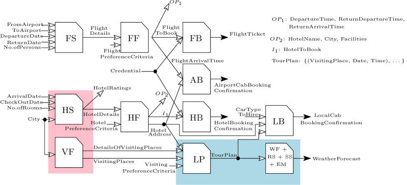
Figure 3: Abstract service generation using fusion

Example 3.10.

Consider the example in Section 2. The construction of an abstract service based on fusion is shown in Figure 3. The colored rectangular boxes show different dependency graphs corresponding to each abstract service created at this level. We start with each service in the previous level and compute the services which are functionally dependent on that service. We assign the values of the QoS parameters of the overall dependency graph to the corresponding abstract service as discussed above. The number of services to be considered for composition now reduces from 16 to 14 after this abstraction step is executed. $\blacksquare$

3.4.1 Composition with abstract services after fusion

For constructing the composition on the abstract service set obtained after fusion, we use the notion of a sub-service, which we formally define below.

Definition 3.7.

[Sub-service: ] ${\cal{S}}^{(4)}_{i}$ is a sub-service of ${\cal{S}}^{(4)}_{j}$, if the set of services corresponding to ${\cal{S}}^{(4)}_{i}$ is a subset of the set of services corresponding to ${\cal{S}}^{(4)}_{j}$. $\blacksquare$

Once the query comes into the system, the dependency graph is constructed. While constructing the dependency graph using the abstract services in $S^{(4)}$, if a service $s\in S^{(4)}$ is used to construct the graph, no sub-service of $s$ is used for the dependency graph construction. Though this abstraction does not reduce the number of abstract services in this level, the size of the dependency graph reduces due to elimination of the sub services. Similar to the third level of abstraction, here also we cannot provide any QoS optimality guarantee on the composite solution. The preservation, soundness and the no-loss theorems still continue to hold.

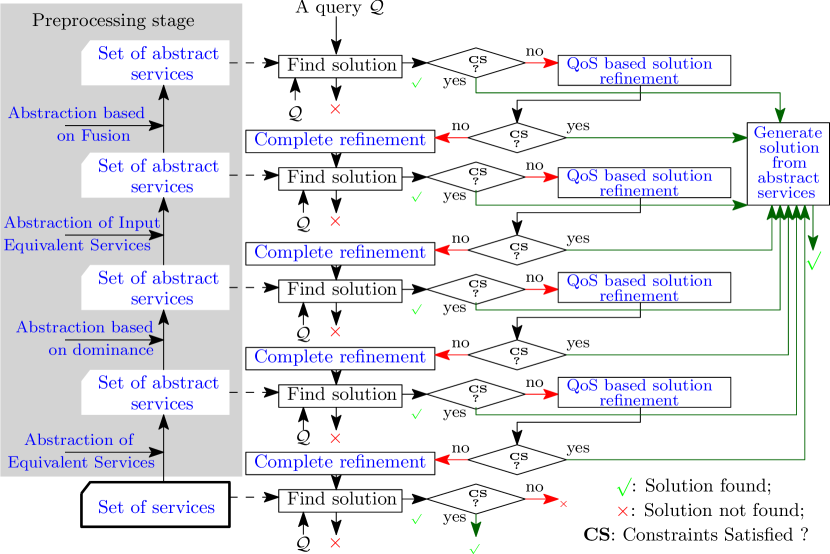
Figure 4: Flow of composition

3.4.2 The Final refinement step

We first discuss QoS based solution refinement followed by the complete refinement. This involves the following:

• We start traversing the solution in the forward direction. We start with the query inputs and find the services that are activated by the query inputs. We then find the services that are activated by the query input as well as the outputs of the services that we have already considered. In this way we proceed until we get back the set of query outputs.

• Once we encounter an abstract service ${\cal{S}}^{(4)}_{i}$ whose corresponding dependency graph consists of more than one service, we traverse the dependency graph and remove all the services which are redundant to solve the given query, i.e., without which the query can still be answered. We then compute the values of the QoS parameters and assign these to ${\cal{S}}^{(4)}_{i}$.

• We recompute the QoS parameters of the solution.

The QoS based solution refinement technique above deals with the $4^{th}$ level abstract services corresponding to each $3^{rd}$ level abstract service of the solution. Therefore, after the QoS based solution refinement step, we end up having the solution constructed over the $3^{rd}$ level abstract services. In the complete refinement strategy, we replace the abstract services by the services in the third level of abstraction in the dependency graph and compute the solution.

3.5 The overall flow

Figure 4 shows the complete flow of our architecture. The Find solution block generates $\times$, when no solutions are found that satisfy the functional dependency and generates $\surd$, if at least one solution is found which satisfies the functional dependency. At any level, once we have the abstract set of services, we can use any standard technique for service composition. Once we get a solution in terms of the abstract services, we need to return the solution in terms of the original services. This can be done by replacing the abstract service in the solution at any level with the original services it represents at the previous level, continuing to the first level. Algorithm 7 shows the the solution reconstruction.

Algorithm 7 SolutionConstruction

1:Input: Solution in terms of abstract services (Sol)

2:Output: Solution in terms of original services

3:for each service $s\in Sol$ do $\triangleright$ $s\in S^{(4)}$

4:    Replace $s$ by the corresponding dependency graph;

5:end for

6:for each service $s\in Sol$ do $\triangleright$ $s\in S^{(3)}$

7:    Replace by the set of services corresponding to $s$;

8:end for

9:for each service $s\in Sol$ do $\triangleright$ $s\in S^{(2)}$

10:    Replace by the dominant service corresponding to $s$;

11:end for

12:for each service $s\in Sol$ do $\triangleright$ $s\in S^{(1)}$

13:    Replace by the service corresponding to $s$ whose QoS parameters are assigned to $s$;

14:end for

4 Experimental Results

Our proposed algorithms were implemented in Java (version 1.7.0_60, 32 bit). All experiments were performed on a 2.53GHz machine with 4GB DDR3 RAM.

4.1 Data sets

We evaluated our methods on the following data sets:

• 5 public repositories of the WSC-2009 [18] dataset

• 19 repositories of the ICEBE-2005 WSC [16] dataset

• An extended version of the description in Section 2.

To demonstrate the power of abstraction and the strength of our methods, we implemented our proposal on top of i) a single QoS aware optimal composition algorithm [19], ii) a multiple QoS aware optimal composition algorithm [12] and iii) a heuristic approach [9]. In the following subsections, we show the performance gain enabled by our method over all the cases. In our experiments, we considered the following problems for a given query:

• Generating all feasible solutions

• Generating a solution with a single QoS parameter

• Generating a solution with multiple parameters

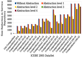
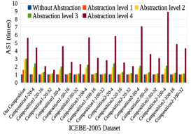
(a) (b) (c)

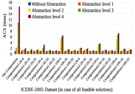
Figure 5: ICEBE dataset: (a)No. of services reduction in repository (b) ASI in dependency graph (c) ACS to construct dependency graph

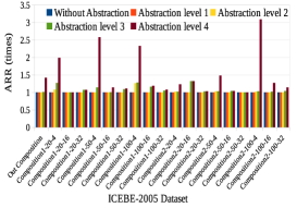
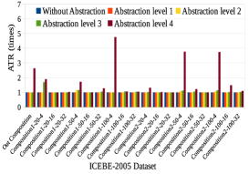
(a) (b) (c)

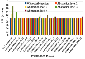
Figure 6: ICEBE dataset (a) ARR (b) ATR (c) AIR

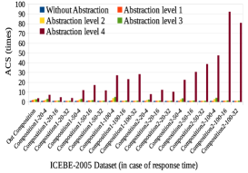
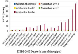
(a) (b) (c)

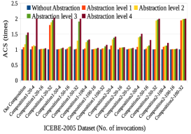
Figure 7: ICEBE dataset average speedup to construct the solution (a) response time aware (b) throughput aware (c) no. of invocations aware

4.2 Evaluation

We first discuss the performance metrics considered for comparison between the approaches.

$\text{Average response time ratio (ARR)}=AVG_{{\cal{Q}}}(\frac{\text{RT computed with abstraction}}{\text{RT computed without abstraction}})$

Average throughput ratio (ATR) = $AVG_{{\cal{Q}}}(\frac{\text{TR computed without abstraction}}{\text{TR computed with abstraction}})$

Average no. of invocations ratio (AIR) = $AVG_{{\cal{Q}}}(\frac{\text{NI computed with abstraction}}{\text{NI computed without abstraction}})$

Average size improvement (ASI) = $AVG_{{\cal{Q}}}(\frac{\text{NSD without abstraction}}{\text{NSD with abstraction}})$

Average computation speedup (ACS) = $AVG_{{\cal{Q}}}(\frac{\text{CT without abstraction}}{\text{CT with abstraction}})$

where, RT, TR, NI, CT, NSD and AVG stand for response time, throughput, the number of invocations, computation time, the number of services in the dependency graph and average respectively and $\cal{Q}$ represents the set of queries.

TABLE I: ICEBE-2005_Composition1 dataset: with multiple QoS constraints

Data	#	Abstraction	# memory out	Avg. composition
sets	queries	level	errors	time (ms)
		0	7	12195
20-4	11	1	4	3662.26
		2	0	4214.36
		3	0	2521.0
		4	0	59.64
		0, 1, 2, 3	11	-
20-16	11	4	1	17095.3
		0, 1, 2, 3	11	-
20-32	11	4	6	452.804
		0, 1	11	-
50-4	11	2	7	13868.5
		3	6	9076.804
		4	0	29.18
		0, 1, 2, 3	11	-
50-16	11	4	1	3222.604
		0, 1. 2, 3	11	-
50-32	11	4	3	1844.37
		0, 1	11	-
100-4	11	2	10	115.94
		3	10	232
		4	0	27.637
		0, 1, 2, 3, 4	11	-
100-16	11	4	0	826.397
		0, 1, 2, 3	11	-
100-32	11	4	1	12015.99

TABLE II: ICEBE_2005_Composition2 dataset: with multiple QoS constraints

Data	#	Abstraction	# memory out	Avg. composition
sets	queries	level	errors	time (ms)
		0, 1	11	-
20-4	11	2	10	67.496
		3	10	7.095
		4	0	83.73
		0, 1, 2, 3	11	-
20-16	11	4	1	1874.09
		0, 1, 2, 3	11	-
20-32	11	4	4	1983.245
		0, 1	11	-
50-4	11	2	10	27.5
		3	10	3.894
		4	0	136.82
		0. 1, 2, 3	11	-
50-16	11	4	2	747.36
		0, 1, 2, 3	11	-
50-32	11	4	4	34928.85
		0, 1, 2, 3	11	-
100-4	11	4	10	777.97
		4	7	197.321
		0, 1, 2, 3	11	-
100-16	11	4	6	2737.91
		0, 1, 2, 3	11	-
100-32	11	5	4	234981.35

We now discuss the evaluation result on 3 different datasets.

4.2.1 Evaluation on ICEBE WSC-2005 Benchmark dataset

Figure 5(a) shows the reduction in the number of services in the service repository across different abstraction levels for the ICEBE-2005 WSC dataset. This is achieved at preprocessing / design time, before arrival of a query. As evident from the figure, the number of services reduces in each level except in the last level (as discussed in Section 3).

We first discuss the performance gain achieved by our method at runtime, when implemented on top of [19]. Figure 5(b) shows the average reduction in the number of services in the dependency graph across different abstraction levels in response to a set of 11 queries that are provided as part of the ICEBE dataset. The X axis of the figure represents the dataset, while the Y axis represents ASI across different abstraction levels. As evident from the figure, there is a significant reduction in the number of services in each level, the average reduction across different levels are 1.04, 1.39, 4.05, 4.13 times respectively. It is worth noting that though in the last abstraction level, the reduction in the number of services in the service repository is not visible, however, the reduction is quite significant (4.13 times on an average) in dependency graph construction in response to a query. Figure 5(c) shows ACS achieved in dependency graph construction across different abstraction levels, the average speedup gained across different levels are 1.21, 1.9, 2.64, 3.13 times respectively.

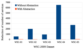
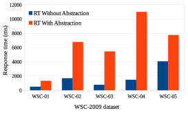
(a) (b) (c)

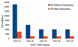
Figure 8: WSC-2009 dataset: (a) Size reduction in dependency graph (b) Response time (c) Throughput

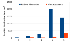
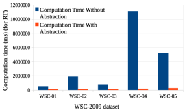
(a) (b) (c)

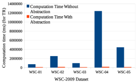
Figure 9: WSC-2009 dataset: (a) Dependency graph construction time (b) Computation time for RT (c) Computation time for TR

Since our approach solves the composition problem on the abstract service groups, there is not always a guarantee of optimal solution generation, for the second abstraction level onwards, as discussed in Section 3. We show the degradation in QoS values empirically on standard benchmark datasets in presence of these abstractions. The ICEBE WSC-2005 dataset does not contain values of the QoS parameters of the services. Therefore, for each service we generated the values of the response time and throughput following a normal distribution. Figure 6(a) shows ARR across different abstraction levels in response to the 11 queries. Figure 7(a) shows the ACS achieved in constructing the optimal response time with different abstraction levels on top of [19]. Evidently, there is a significant speedup gain in computation time as compared to the degradation in solution quality. For 2 out of the 19 datasets, our method is able to derive the optimal response time even after all four levels of abstraction.

Figure 6(b) shows the ATR across different abstraction levels in response to the 11 queries. Figure 7(b) shows the corresponding ACS with different abstraction levels on top of [19]. In this case as well, for 3 out of the 19 datasets, we still get the optimal throughput after all abstractions.

We now compare our proposal with a heuristic method [9], which considers the number of invocations as a QoS parameter. Figure 6(c) shows a plot of AIR with different abstraction levels in response to the same set of 11 queries, while Figure 7(c) shows the corresponding ACS achieved on top of [9]. Evidently, there is a significant speedup gain in computation time as compared to the change in the number of invocations. In this case, our methods generate the same solution (i.e., without degrading the average number of invocations) for 13 out of the 19 datasets after all abstractions.

Finally, we consider multiple QoS parameters for the ICEBE-2005 datasets and the results are shown in Tables I and II. We consider response time, reliability, availability, invocation cost and the number of service invocations as QoS parameters. The QoS values of each service are generated randomly. Columns 2, 3, 4 and 5 of the table represent the number of queries, the abstraction level, the number of memory out errors for each abstraction and average time for composition respectively. As evident from the tables, the average composition time decreases considerably as the abstraction level increases. It may be noted that in many cases, the ILP-based optimal algorithm [12] gets memory out errors, as shown in Tables I and II. For example, consider the 20-4 dataset of Table I. For the case without abstraction, the ILP fails to generate any solution (because of memory-out error) for 7 queries. However, as the abstraction level increases, the number of memory out error decreases.

4.2.2 Evaluation on the WSC-2009 dataset

Figure 8(a) shows the reduction achieved in the number of services for dependency graph construction with and without abstraction in response to a query, while Figure 9(a) shows the corresponding computation speedup. It is evident from the figures, in presence of abstraction, the solution generation time is considerably less. For the WSC-2009 dataset, we did not observe any service reduction for first 3 levels of abstraction and hence, omitted them.

WSC-2009 contains the values of response time and throughput of the services. Figure 8(b) shows the response times with and without abstraction in response to a query in our method, while Figure 9(b) shows the computation time needed to construct the optimal response time with and without abstraction on top of [19]. As evident from the figures, there is a significant speedup gain in computation time as compared to the degradation in optimal response time. A similar gain is achieved for throughput. Figure 8(c) shows the throughput with and without abstraction in response to a query and Figure 9(c) shows the corresponding computation time required to generate the optimal throughput with and without abstraction using [19].

4.2.3 Evaluation on a synthetic dataset

We extended the service description discussed in Section 2. We considered 30 different service categories. Each service category performs a specific operation / task. Under each category, there are 3 or 4 different sub categories. Each sub category is selected based on input-output parameters. The services under a specific sub category have identical set of inputs and outputs. We used an in-house web crawler and the open travel alliance dataset to get the number of services for some service categories (e.g., searchFlight, bookFlight, searchHotel, bookHotel, forecastWeather, bookAirportTransport, bookLocalTransport, searchRestaurant etc). For the remaining service categories, we randomly generated the number of services. Once this was done, we randomly divided the services into multiple sub categories. We considered the query as discussed in Section 2. The total number of services in the service repository was 2461. We used the QWS dataset to assign the QoS values to the services. The QWS dataset has 8 different QoS parameters and more than 2500 services. From the QWS dataset, we randomly selected 2461 services and the corresponding QoS values were assigned to the services in our repository.

TABLE III: Synthetic dataset: Performance of our approach

SL	Speed up (times)	Abstraction Level
1	728	4
2	722	4
3	513	4
4	426	3
5	196	2
6	122	1
7	69	1
8	1.23	1
9	-6.45	0
10	-13	0

The service repository initially contained 2461 services. We had 82, 30, 24 and 24 services after the first, second, third and fourth levels of abstraction respectively. The dependency graph with respect to the query consisted of 1423 services. We had 35, 12, 10 and 8 services after the first, second, third and fourth levels of abstraction respectively. We first generated a random QoS constraint such that the fourth level abstract services can produce the solution satisfying all QoS constraints. We gradually tightened the constraints, till no solutions existed, as shown in the 10^th row of Table III. Table III presents the performance of our approach. A larger row number indicates tighter constraints. Column 2 of Table III represents the speed up with respect to the solution generated without any abstraction, Column 3 presents at which abstraction level, we get a solution to the query satisfying all QoS constraints. As evident from the table, as abstraction level decreases, the speed up also decreases. In the final two rows (8^th and 9^th), the solution is generated without abstraction, therefore we observe performance degradation.

5 Related Work

A significant amount of work has been done by considering different perspectives of service composition and discovery [1, 24, 25, 26]. The primary objective of service composition methods has been the computation of the optimal service composition result [5, 6, 19, 27] considering functional and non-functional attributes. The optimality requirement however, in general, has proved to be an expensive requirement [3, 11] for service composition solutions. Therefore, heuristic solutions [28, 9, 29, 30] have been proposed, that have the ability to generate solutions fast and handle large and complex service spaces [3], but have sub-optimal solution quality [31, 32]. Table IV presents a summary of some of the popular approaches in service composition based on different factors considered.

TABLE IV: Description of State-of-the-Art Approaches

References	Focus	Single /	QoS Params	Static /	Optimal /	Deterministic /	Method
		Multiple Params	Considered	Dynamic	Heuristic	probabilistic
[3]	Scalability	Multiple	RT, EP	Static	QoS constrained	Deterministic	Constraint Satisfaction Problem
[5]	Redundancy control	Both	RT, TR	Static	Optimal	Deterministic	Graph based search
[6]	Service Composition	Multiple	Cost, RT, TR, AV	Static	Optimal + QoS constrained	Stochastic	ILP, Greedy Heuristic
					Heuristic
[7]	Service Composition	Single	RT, TR	Static	Optimal	Deterministic	Graph based search
[9]	Service Composition	Single	NI	Static	Heuristic	Deterministic	A*
[11]	Scalability	Both	RT, TR, NI, RE, AV	Static	Heuristic	Deterministic	Local Search
[12]	Service Composition	Multiple	RT, TR, NI, RE, AV	Static	Optimal + QoS constrained	Stochastic	ILP, A*, Local Search
					Heuristic
[19, 27]	Redundancy control	Single	RT, TR	Static	Optimal	Deterministic	Graph based search
[33]	Service Composition	Multiple	Price, Duration, RE, RP, AV	Static	Optimal	Deterministic	ILP
[30]	Transactional Driven	Multiple	Price, Duration	Static	Heuristic +	Deterministic	Local optimization
	Service Composition		SR, RP, AV		Transactional Constraint		algorithm
[34]	Top-k Service	Single	RT, TR	Static	Optimal	Deterministic	Backtrack search, DFS
	Composition						parallel algorithm
[35]	Service Composition	Single	NI	Static	Optimal	Deterministic	AI planning and
							network optimization
[36]	Service Composition	Single	RT, TR	Static	Optimal	Deterministic	Graph based search
[37]	Service Composition	Single	RT, EP	Static	Optimal	Deterministic	Genetic Algorithms
[38]	Service Composition	Multiple	Cost, Duration, RP, RE, AV	Dynamic	Optimal	Deterministic	ILP
[40]	Service Composition	Single	RT, TR	Static	Optimal	Deterministic	Graph search, planning algorithm
[31, 32]	Service Composition	Multiple	Price, Duration, RP, ST, AV	Static	QoS constrained	Deterministic	Constraint Satisfaction Problem
[41, 22]	Service Composition	Multiple	RT, TR	Static	Heuristic	Deterministic	Anytime algorithm, Graphplan
[28]	Multi granularity	Multiple	Time, Price, RE	Static	Heuristic	Deterministic	Backtracking-based algorithm,
	Service Composition						Genetic Algorithms
[42]	Service Composition in	Multiple	AV, RT, Cost	Dynamic	Optimal	Deterministic	Reinforcement learning,
	Uncertain Environments						Markov Decision Proces
Note: RT: ResponseTime, TR: Throughput, RE: Reliability, AV: Availability, ST: Success Rate, RP: Reputation, NI: Number of invocations EP: Execution Price

In contrast to existing literature, we propose an abstraction refinement based approach that aims to expedite the solution construction time by working on a reduced search space. Our approach provides a scalable way of pruning the dependency graphs that are considered by any composition solution. Our method has the ability to work on top of any service composition method, and improve its performance. Thus, we do not propose a new service composition solution, rather a framework on top of existing ones. This distinguishes our approach from the existing ones.

6 Conclusion and future directions

This paper presents an abstraction-refinement based approach to expedite a service composition algorithm. For a large dataset, the abstraction can be very effective. It reduces the memory requirement and improves performance. As evident from the experimental results, this mechanism is indeed more efficient on average, while having the same worst case performance when implemented on any method. Our method is generic enough to be applied to any QoS parameter in service composition. As future work, we are currently working on extending our proposal to develop more sophisticated refinement techniques and incorporating semantics based abstraction. We believe that our work will open up a lot of new research directions in the general paradigm of abstraction refinement based composition.

Soumi Chattopadhyay is a Ph.D student at the Advanced Computing and Microelectronics Unit, Indian Statistical Institute Kolkata. She completed her under-graduate studies from West Bengal University of Technology, and Master’s from the Indian Statistical Institute Kolkata – all in Computer Science. Soumi’s research interests are in distributed and services computing.

Ansuman Banerjee is an Associate Professor at the Advanced Computing and Microelectronics Unit, Indian Statistical Institute Kolkata. He received his B.E. from Jadavpur University, and M.S. and Ph.D. degrees from the Indian Institute of Technology Kharagpur – all in Computer Science. His research interests include formal methods for services computing.

References

- [1] C. Jatoth et al., “Computational intelligence based qos-aware web service composition: A systematic literature review,” TSC, vol. PP, no. 99, pp. 1–1, 2015.
- [2] N. Milanovic and M. Malek, “Current solutions for web service composition,” IEEE Internet Computing, vol. 8, no. 6, p. 51, 2004.
- [3] F. Lecue and N. Mehandjiev, “Towards scalability of quality driven semantic web service composition,” in ICWS, 2009, pp. 469–476.
- [4] Y. Wu et al., “A multilevel index model to expedite web service discovery and composition in large-scale service repositories,” IEEE TSC, vol. 9, no. 3, pp. 330–342, 2016.
- [5] P. Rodriguez-Mier et al., “Hybrid optimization algorithm for large- scale qos-aware service composition,” TSC, 2015.
- [6] D. Schuller et al., “Cost-driven optimization of complex service- based workflows for stochastic qos parameters,” in ICWS, 2012, pp. 66–73.
- [7] M. Aiello et al., “Optimal qos-aware web service composition,” in 2009 IEEE ICCEC, 2009, pp. 491–494.
- [8] D. Papadias et al., “An optimal and progressive algorithm for skyline queries,” in SIGMOD. ACM, 2003, pp. 467–478.
- [9] P. Rodriguez-Mier et al., “Automatic web service composition with a heuristic-based search algorithm,” in ICWS, 2011, pp. 81–88.
- [10] R. Aggarwal et al., “Constraint driven web service composition in meteor-s,” in SCC, 2004, pp. 23–30.
- [11] S. Chattopadhyay et al., “A scalable and approximate mechanism for web service composition,” in ICWS. IEEE, 2015, pp. 9–16.
- [12] S. Chattopadhyay and A. Banerjee, “QSCAS: qos aware web service composition algorithms with stochastic parameters,” in ICWS, 2016, pp. 388–395.
- [13] A. Klein et al., “Efficient heuristic approach with improved time complexity for qos-aware service composition,” in ICWS, 2011, pp. 436–443.
- [14] M. Alrifai et al., “Combining global optimization with local selec- tion for efficient qos-aware service composition,” in WWW, 2009, pp. 881–890.
- [15] P. Hennig et al., “Highly scalable web service composition using binary tree-based parallelization,” in ICWS, 2010, pp. 123–130. E. Clarke et al., “Counterexample-guided abstraction refinement,” in CAV, 2000, pp. 154–169.
- [16] K. S. et al., “The web services challenge,” in ICEBE, 2005.
- [17] . Available: http://www.comp.hkbu.edu.hk/simctr/wschallenge/
- [18] S. Kona et al., “Wsc-2009: a quality of service-oriented web services challenge,” in IEEE ICCEC, 2009.
- [19] Y.-M. Xia et al., “Web service composition integrating qos opti- mization and redundancy removal,” in ICWS, 2013, pp. 203–210.
- [20] M. Alrifai et al., “A hybrid approach for efficient web service composition with end-to-end qos constraints,” ACM TWEB, vol. 6, no. 2, p. 7, 2012.
- [21] R. Eshuis et al., “Flexible construction of executable service compo- sitions from reusable semantic knowledge,” TWEB, vol. 10, no. 1, pp. 5–, 2016.
- [22] Y. Yan and M. Chen, “Anytime qos-aware service composition over the graphplan,” Springer SOCA, vol. 9, no. 1, pp. 1–19, 2015.
- [23] R. T. Marler and J. S. Arora, “Survey of multi-objective opti- mization methods for engineering,” Structural and multidisciplinary optimization, vol. 26, no. 6, pp. 369–395, 2004.
- [24] W. Jiang et al., “Continuous query for qos-aware automatic service composition,” in ICWS. IEEE, 2012, pp. 50–57.
- [25] S. Zhang et al., “Selecting top-k composite web services using preference-aware dominance relationship,” in ICWS, 2013, pp. 75– 82.
- [26] M. Mehdi et al., “Trustworthy web service selection using proba- bilistic models,” in ICWS, 2012, pp. 17–24.
- [27] M. Chen and Y. Yan, “Redundant service removal in qos-aware service composition,” in ICWS, 2012, pp. 431–439.
- [28] Q. Wu et al., “Qos-aware multigranularity service composition: Modeling and optimization,” IEEE TSMC, vol. 46, pp. 1565–1577, 2016.
- [29] I. Guidara et al., “Heuristic based time-aware service selection approach,” in ICWS. IEEE, 2015, pp. 65–72.
- [30] J. El Hadad et al., “Tqos: Transactional and qos-aware selection algorithm for automatic web service composition,” IEEE TSC, vol. 3, no. 1, pp. 73–85, 2010.
- [31] X. Song et al., “A workflow framework for intelligent service composition,” FGCS, vol. 27, no. 5, pp. 627–636, 2011.
- [32] M. Pistore et al., “Automated composition of web services by planning at the knowledge level,” in IJCAI, 2005, pp. 1252–1259.
- [33] L. Zeng et al., “Quality driven web services composition,” in WWW. ACM, 2003, pp. 411–421.
- [34] S. Deng et al., “Top-automatic service composition: A parallel method for large-scale service sets,” IEEE TASE, vol. 11, no. 3, pp. 891–905, 2014.
- [35] S.-C. Oh et al., “Effective web service composition in diverse and large-scale service networks,” IEEE TSC, vol. 1, no. 1, pp. 15–32, 2008.
- [36] Y. Yan et al., “A qos-driven approach for semantic service compo- sition,” in IEEE ICCEC. IEEE, 2009, pp. 523–526.
- [37] F. Lécué, “Optimizing qos-aware semantic web service composi- tion,” in ICWS, 2009.
- [38] F. Paganelli et al., “A qos-aware service composition approach based on semantic annotations and integer programming,” IJWIS, vol. 8, no. 3, pp. 296–321, 2012.
- [39] E. Clarke et al., “Counterexample-guided abstraction refinement,” in CAV, 2000, pp. 154–169.
- [40] F. Wagner et al., “Qos-aware automatic service composition by applying functional clustering,” in ICWS. IEEE, 2011, pp. 89–96.
- [41] Y. Yan et al., “Anytime qos optimization over the plangraph for web service composition,” in SAC, 2012, pp. 1968–1975.
- [42] A. Mostafa and M. Zhang, “Multi-objective service composition in uncertain environments,” IEEE TSC, vol. PP, no. 99, pp. 1–1, 2015.