Lopsided Approximation of Amoebas

Abstract.

The amoeba of a Laurent polynomial is the image of the corresponding hypersurface under the coordinatewise log absolute value map. In this article, we demonstrate that a theoretical amoeba approximation method due to Purbhoo can be used efficiently in practice. To do this, we resolve the main bottleneck in Purbhoo’s method by exploiting relations between cyclic resultants. We use the same approach to give an approximation of the Log preimage of the amoeba of a Laurent polynomial using semi-algebraic sets. We also provide a SINGULAR/Sage implementation of these algorithms, which shows a significant speedup when our specialized cyclic resultant computation is used, versus a general purpose resultant algorithm.

1. Introduction

Consider a Laurent polynomial

$$f(\mathbf{z})=\sum_{j=1}^{d}b_{j}\,\mathbf{z}^{\alpha(j)},$$ (1.1)

where ${\color[rgb]{0,0,1}\mathbf{z}}:=(z_{1},\ldots,z_{n})$. We denote by ${\color[rgb]{0,0,1}{\rm Var}(f)}$ the hypersurface defined by $f$ in the maximal open torus ${\color[rgb]{0,0,1}(\mathbb{C}^{*})^{n}}:=(\mathbb{C}\setminus\{0\})^{n}$ of ${\mathbb{C}}^{n}$.

Definition 1.1.

The log absolute value map is given by

$${\color[rgb]{0,0,1}{\operatorname{Log}}\ |\cdot|}\colon\ \left(\mathbb{C}^{*}\right)^{n}\to\mathbb{R}^{n},\quad(z_{1},\ldots,z_{n})\mapsto(\log|z_{1}|,\ldots,\log|z_{n}|)\,.$$ (1.2)

The amoeba ${\color[rgb]{0,0,1}{\mathscr{A}}(f)}$ of $f$ is defined as ${\operatorname{Log}}\ |{\rm Var}(f)|$. The unlog amoeba ${\color[rgb]{0,0,1}{\mathscr{U}}(f)}$ of $f$ is defined as $|{\rm Var}(f)|$, where

$${\color[rgb]{0,0,1}|\cdot|}\colon\ \left(\mathbb{C}^{*}\right)^{n}\to\mathbb{R}^{n},\quad(z_{1},\ldots,z_{n})\mapsto(|z_{1}|,\ldots,|z_{n}|)\,.$$

$\hexagon$

Gelfand, Kapranov and Zelevinsky introduced amoebas in [GKZ94, Definition 6.1.4] in the context of toric geometry. Since then, amoebas have been used in different areas such as complex analysis [FPT00, PR04], real algebraic curves [Mik00], statistical thermodynamics [PPT13], and nonnegativity of real polynomials [IdW16]. Overviews on amoeba theory include [dW17, Mik04, PT05].

The usefulness of amoebas motivates the problem of finding an efficient algorithm for computing them. Since ${\operatorname{Log}}|\cdot|$ is a non-algebraic map, ${\mathscr{A}}(f)$ is not a semi-algebraic set in general. The amoeba ${\mathscr{A}}(f)$ is, however, a semi-analytic set. The absolute value map, on the other hand, is a real algebraic map. Therefore, the unlog amoeba ${\mathscr{U}}(f)$ is a real semi-algebraic set. Hence, the ideal solution to the problem of amoeba computation can be described as follows.

Given a Laurent polynomial $f\in\mathbb{C}[\mathbf{z}^{\pm 1}]$, efficiently compute a real semi-algebraic description of the unlog amoeba ${\mathscr{U}}(f)$.

Theobald was the first to tackle computational aspects of amoebas in [The02]. He described, in the case $n=2$, methods to compute a superset of the boundary of ${\mathscr{A}}(f)$ called the contour of ${\mathscr{A}}(f)$. Later, his method was extended by Schroeter and the fourth author in [SdW13], who provide a method to test whether a contour point of ${\mathscr{A}}(f)$ belongs to the boundary of ${\mathscr{A}}(f)$ in the case when the hypersurface defined by $f$ is smooth.

An approach, different than Theobald’s, for computing amoebas arises from following problem.

Problem 1.2 (The Membership Problem).

Let $f\in\mathbb{C}[\mathbf{z}^{\pm 1}]$ and $|\mathbf{v}|\in\mathbb{R}^{n}$. Provide a certificate $C$ such that if $C(|\mathbf{v}|)$ is true, then ${\operatorname{Log}}|\mathbf{v}|\notin{\mathscr{A}}(f)$.

The membership problem was addressed by Purbhoo in [Pur08], using the notion of lopsidedness; see Definition 1.3. A second approach for certifying non-membership of a point in ${\mathscr{A}}(f)$ was provided by Theobald and the fourth author in [TdW15] using semidefinite programming and sums of squares. A rough but quick method to approximate amoebas was given by Avendaño, Kogan, Nisse and Rojas [AKNR13] via tropical geometry. In [BKS16], Bogdanov, Kytmanov and Sadykov computed amoebas in dimensions two and three, with focus on amoebas with the most complicated topology possible. We remark that even for univariate polynomials deciding the membership problem is NP-hard [AKNR13, Section 1.2].

The main aim of this article is to make the results in [Pur08] effective and efficient in practice.

Definition 1.3 ([Rul03, Page 24] and [Pur08, Definition 1.2]).

Let $f$ be as in (1.1). We say that $f$ is lopsided at a point ${\operatorname{Log}}|\mathbf{v}|\in\mathbb{R}^{n}$ if there exists an index $k\in\{1,\ldots,d\}$ such that

$$\left|b_{k}\,\mathbf{v}^{\alpha(k)}\right| > \sum_{j\in\{1,\ldots,d\}\setminus\{k\}}\left|b_{j}\,\mathbf{z}^{\alpha(j)}\right|.$$ (1.3)

The lopsided amoeba of $f$ is defined by

$${\color[rgb]{0,0,1}{\mathscr{L}}(f)} := \big{\{}{\operatorname{Log}}|\mathbf{v}|\in\mathbb{R}^{n}\ \big{|}\ f\text{ is not lopsided at }{\operatorname{Log}}|\mathbf{v}|\big{\}}.$$

$\hexagon$

It is not hard to see that ${\mathscr{A}}(f)\subseteq{\mathscr{L}}(f)$; the special case $n=1$ of this result was proven in the nineteenth century, in an equivalent formulation, by Pellet [Pel81]. We remark that, in general, ${\mathscr{A}}(f)\neq{\mathscr{L}}(f)$.

Following Purbhoo, we introduce

$${\color[rgb]{0,0,1}{\rm CycRes}(f;r)}:=\ \prod_{k_{1}=0}^{r-1}\cdots\prod_{k_{n}=0}^{r-1}f\left(e^{2\pi ik_{1}/r}z_{1},\ldots,e^{2\pi ik_{n}/r}z_{n}\right)$$ (1.4)

$$\qquad={\operatorname{Res}}_{u_{n}}\left({\operatorname{Res}}_{u_{n-1}}\left(\ldots{\operatorname{Res}}_{u_{1}}(f(u_{1}z_{1},\ldots,u_{n}z_{n}),u_{1}^{r}-1),\ldots,u_{n-1}^{r}-1\right),u_{n}^{r}-1\right),$$

where ${{\color[rgb]{0,0,1}{\operatorname{Res}}_{x}(g,h)}}$ denotes the resultant of the polynomials $g$ and $h$ with respect to the variable $x$. If $g=g(x)$ is a univariate polynomial, then ${\operatorname{Res}}_{x}(g,x^{r}-1)$ is called a cyclic resultant of $g$.

Note that ${\rm CycRes}(f;r)$ is a Laurent polynomial in $z_{1},\dots,z_{n}$. The informal version of [Pur08, Theorem 1] states that the limit as $r\to\infty$ of ${\mathscr{L}}({\rm CycRes}(f;r))$ is ${\mathscr{A}}(f)$; see Section 2.2 for more information.

The main obstacle in turning Purbhoo’s result into an efficient approximation method for amoebas is the difficulty in computing the polynomials ${\rm CycRes}(f;r)$. The degree and the number of terms of ${\rm CycRes}(f;r)$ grow exponentially with $r$, but more importantly, the methods used by computer algebra systems to find resultants fail to take advantage of the sparseness of the polynomials $u_{i}^{r}-1$, and are therefore manifestly inefficient when applied to ${\rm CycRes}(f;r)$.

Our main results are as follows.

1. We give a fast method to compute the cyclic resultant ${\rm CycRes}(f;2r)$ from ${\rm CycRes}(f;r)$ omitting all intermediate steps ${\rm CycRes}(f;r+1),\ldots,{\rm CycRes}(f;2r-1)$; see Section 3 for details. We provide an experimental comparison of the runtimes using these quick resultants versus a general purpose resultant algorithm in Table 2. We also give the complexity of our specialized algorithm for computing (certain) cyclic resultants, verifying our experimental conclusion that this method is significantly faster than the best resultant algorithm for real polynomials (Remark 3.5).

2. We provide an algorithm to approximate the unlog amoeba by semialgebraic sets, see Theorem 6.1 and Algorithm 6.2.

Purbhoo’s Amoeba Approximation Theorem is the main ingredient in the proof of Theorem 6.1 and in Algorithm 6.2. Using toric geometry, we also show that there exists a natural correspondence between the boundary components of lopsided amoebas and the boundary components of linear amoebas, where the latter are well understood due to Forsberg, Passare, and Tsikh [FPT00]; see Section 5 for further details.

Lemma 3.3 allows us to compute cyclic resultants for powers $r=2^{k}$ using a divide and conquer algorithm. Note that several prominent algorithms are built on a similar approach, for example the Cooley–Tukey algorithm for the Fast Fourier Transformation [CT65].

As a companion to this work we provide the first implementation of lopsided approximation of amoebas, available here:

http://www.math.tamu.edu/research/dewolff/LopsidedAmoebaApproximation/.

We also provide the data presented in this article on this website. The algorithms in this article are implemented in the computer algebra system Singular [DGPS15] and scripts to provide graphical outputs use the computer algebra system Sage [Dev16].

Outline

This paper is organized as follows. Section 2 contains background on amoebas and lopsided amoebas. Section 3 outlines a fast way of computing certain cyclic resultants. In Section 4 we describe how the algorithm from Section 3 can be used to approximate amoebas. Section 5 provides a geometric interpretation of the lopsided amoeba as the intersection of the amoeba of a toric variety and the amoeba of a hyperplane. In Section 6 we describe how to use results from Sections 3 and 5 to compute semialgebraic sets approximating the amoeba. Finally, Section 7 is devoted to examples.

Acknowledgements

We are very grateful to Alicia Dickenstein for her helpful suggestions, especially on resultants. We also thank Luis Felipe Tabera for his helpful comments. We are grateful to the anonymous referee for their helpful suggestions.

2. Preliminaries

In this section, we review the theory of amoebas and lopsided amoebas which is used in this work.

Recall that throughout this article, $f\in{\mathbb{C}}[\mathbf{z}^{\pm 1}]$ denotes the Laurent polynomial (1.1). We denote by $A$ the support of $f$, namely,

$${\color[rgb]{0,0,1}A}\ :=\ \big{\{}\alpha\in{\mathbb{Z}}^{n}\,\big{|}\,{\bf{z}}^{\alpha}\text{ appears with nonzero coefficient in }f\big{\}}.$$

The Newton polytope of $f$, denoted ${{\color[rgb]{0,0,1}{\rm New}(f)}}$, is the convex hull in ${\mathbb{R}}^{n}$ of the support set $A$ of $f$.

2.1. Amoebas

The complement of the amoeba ${\mathscr{A}}(f)$ is the set ${\mathbb{R}}^{n}\smallsetminus{\mathscr{A}}(f)$. The connected components of ${\mathbb{R}}^{n}\smallsetminus{\mathscr{A}}(f)$ are referred to as the components of the complement of ${\mathscr{A}}(f)$.

Theorem 2.1 ([GKZ94, Chapter 6.1.A, Proposition 1.5, Corollary 1.8]).

For a nonzero Laurent polynomial $f$, the complement ${\mathbb{R}}^{n}\smallsetminus{\mathscr{A}}(f)$ is non-empty. Every component of ${\mathbb{R}}^{n}\smallsetminus{\mathscr{A}}(f)$ is convex and open (with respect to the standard topology).

Forsberg, Passare and Tsikh [FPT00] showed that every component of the complement of an amoeba ${\mathscr{A}}(f)$ can be associated with a specific lattice point in the Newton polytope ${\rm New}(f)$ via the order map:

$${\color[rgb]{0,0,1}\operatorname{ord}}\colon\mathbb{R}^{n}\smallsetminus{\mathscr{A}}(f) \to {\mathbb{R}}^{n},\quad\mathbf{w}\mapsto(u_{1},\ldots,u_{n}),\ \text{ where }$$ (2.1)

$$u_{j} := \frac{1}{(2\pi\sqrt{-1})^{n}}\int_{{\operatorname{Log}}|\mathbf{z}|=\mathbf{w}}\frac{z_{j}\partial_{j}f(\mathbf{z})}{f(\mathbf{z})}\frac{dz_{1}\cdots dz_{n}}{z_{1}\cdots z_{n}}\ \text{ for all }\ 1\leq j\leq n\,.$$

Theorem 2.2 ([FPT00, Propositions 2.4 and 2.5]).

The image of the order map is contained in ${\rm New}(f)\cap\mathbb{Z}^{n}$. Let $\mathbf{w},\mathbf{w}^{\prime}\in{\mathbb{R}}^{n}\smallsetminus{\mathscr{A}}(f)$. Then $\mathbf{w}$ and $\mathbf{w}^{\prime}$ belong to the same component of the complement of ${\mathscr{A}}(f)$ if and only if $\operatorname{ord}(\mathbf{w})=\operatorname{ord}(\mathbf{w}^{\prime})$.

As a consequence of Theorem 2.2, it is possible to define the component of order $\alpha$ of the complement of ${\mathscr{A}}(f)$. We use the following notation:

$${\color[rgb]{0,0,1}E_{\alpha}(f)} := \{\mathbf{w}\in\mathbb{R}^{n}\smallsetminus{\mathscr{A}}(f)\ \mid\ \operatorname{ord}(\mathbf{w})=\alpha\}.$$ (2.2)

2.2. Lopsided Amoebas

We now give a more precise statement of the main result in [Pur08], which was alluded to in the introduction.

Theorem 2.3 ([Pur08, Theorem 1 “rough version”]).

For $r\to\infty$ the family ${\mathscr{L}}({\rm CycRes}(f;r))$ converges uniformly to ${\mathscr{A}}(f)$. More precisely, for every $\varepsilon>0$ there exists an integer $N$ such that for all $r>N$ the lopsided amoeba ${\mathscr{L}}({\rm CycRes}(f;r))$ is contained in an $\varepsilon$-neighborhood of ${\mathcal{A}}(f)$.

Remark 2.4.

The integer $N$ in Theorem 2.3 depends only on $\varepsilon$ and the Newton polytope (or degree) of $f$, and can be computed explicitly from this data. For simplicity, assume that $f$ is a polynomial of degree $d$. Let ${\operatorname{Log}}|\mathbf{v}|\in{\mathbb{R}}^{n}\setminus{\mathscr{A}}(f)$ be of distance at least $\varepsilon$ from the amoeba ${\mathscr{A}}(f)$. Then, by [Pur08, Theorem 1], if $r$ is chosen such that

$$r\varepsilon\ \geq\ (n-1)\log r+\log\left((n+3)2^{n+1}d\right),$$

then it holds that ${\rm CycRes}(f;r)$ is lopsided at the point ${\operatorname{Log}}|\mathbf{v}|$. We will typically be interested in the case $r=2^{k}$. Then, it suffices that

$$\frac{2^{k}}{k}\ \geq\ \frac{C(n,d)}{\varepsilon},$$

where ${\color[rgb]{0,0,1}C(n,d)}:=(n-1)\log 2+\log\left((n+3)2^{n+1}d\right)$ is constant.

If $f$ is lopsided at a point ${\operatorname{Log}}|\mathbf{v}|\in\mathbb{R}^{n}$, then it is straightforward to determine the order of the component of the complement of ${\mathcal{A}}(f)$ which contains ${\operatorname{Log}}|\mathbf{v}|$.

Theorem 2.5 ([FPT00, Proposition 2.7] and [Pur08, Proposition 4.1]).

Let $A\subset\mathbb{Z}^{n}$ and let $f(\mathbf{z})$ be as in (1.1). Assume that $f(\mathbf{z})$ is lopsided at ${\operatorname{Log}}|\mathbf{v}|$ with dominating term $|b_{\alpha^{\prime}}\,\mathbf{z}^{\alpha^{\prime}}|$. Then $\operatorname{ord}({\operatorname{Log}}|\mathbf{v}|)=\alpha^{\prime}$. In particular, if ${\rm CycRes}(f,r)$ is lopsided at ${\operatorname{Log}}|\mathbf{v}|$ with dominating term $|b_{\alpha^{\prime}}\,\mathbf{z}^{\alpha^{\prime}}|$, then $\operatorname{ord}({\operatorname{Log}}|\mathbf{v}|)\cdot r^{n}=\alpha^{\prime}$.

The following useful criterion for lopsidedness is a consequence of the triangle inequality.

Lemma 2.6.

The Laurent polynomial $f({\mathbf{z}})$ is not lopsided at ${\operatorname{Log}}|{\mathbf{z}}|$ if and only if there exist arguments $\theta\in(S^{1})^{d}$ such that $\sum_{j=1}^{d}b_{j}\,e^{\theta_{j}\sqrt{-1}}\,\mathbf{z}^{\alpha(j)}=0.$

3. A Fast Algorithm to Compute Cyclic Resultants

In this section, we provide a fast way of computing certain cyclic resultants.

We recall the Poisson formula for the resultant. If $f(z)$ and $g(z)$ are univariate polynomials, and $g$ has leading coefficient $b$, then

$${\operatorname{Res}}_{z}(f,g) = b^{\deg(f)}\prod_{\{\xi\,\mid\,g(\xi)=0\}}f(\xi).$$ (3.1)

Lemma 3.1.

Let $g\in{\mathbb{C}}[z]$ be a univariate polynomial of degree $\delta$ with leading coefficient $b$, and let $r$ be a positive integer. Then there exists a univariate polynomial $h$ of degree $\delta$ such that

$${\operatorname{Res}}_{u}\big{(}g(zu),u^{r}-1\big{)} = h(z^{r}).$$

Proof.

By (3.1),

$${\operatorname{Res}}_{u}\big{(}g(zu),u^{r}-1\big{)} = \prod_{j=0}^{r-1}g\big{(}e^{2\pi\sqrt{-1}j/r}z\big{)}.$$

Writing $g(z)=b\prod_{\ell=1}^{\delta}(z-\xi_{\ell})$, we have

$${\operatorname{Res}}_{u}\big{(}g(zu),u^{r}-1\big{)} = \prod_{j=0}^{r-1}\,b\prod_{\ell=1}^{\delta}(e^{2\pi\sqrt{-1}j/r}z-\xi_{\ell})$$

$$= b^{r}\prod_{\ell=1}^{\delta}\,\prod_{j=0}^{r-1}(e^{2\pi\sqrt{-1}j/r}z-\xi_{\ell})$$

$$= b^{r}\prod_{\ell=1}^{\delta}(z^{r}-\xi_{\ell}^{r}).$$

Now use $h(z)=b^{r}\prod_{\ell=1}^{\delta}(z-\xi_{\ell}^{r})$. ∎

Lemma 3.2.

Let $h\big{(}z^{2^{k}}\big{)}={\operatorname{Res}}_{u}\big{(}g(zu),u^{2^{k}}-1\big{)}$ be as in Lemma 3.1. Then

$${\operatorname{Res}}_{u}\big{(}g(zu),u^{2^{k}}+1\big{)} = h(-z^{2^{k}}).$$

Proof.

Note that the roots of $u^{2^{k}}+1$ are exactly the roots of $u^{2^{k}}-1$ multiplied by $e^{2\pi\sqrt{-1}/(2^{k+1})}$. Therefore, by (3.1),

$${\operatorname{Res}}_{u}\big{(}g(zu),u^{2^{k}}+1\big{)} =\prod_{j=0}^{2^{k}-1}g\left(e^{2\pi\sqrt{-1}j/2^{k}}e^{2\pi\sqrt{-1}/2^{k+1}}z\right)$$

$$=h\left((e^{2\pi\sqrt{-1}/2^{k+1}}z)^{2^{k}}\right)$$

$$=h\big{(}-z^{2^{k}}\big{)}.\qed$$

Lemma 3.3.

The following identity holds.

$${\operatorname{Res}}_{u}\big{(}g(zu),u^{2^{k+1}}-1\big{)} = {\operatorname{Res}}_{u}\big{(}g(zu),u^{2^{k}}-1\big{)}\cdot{\operatorname{Res}}\big{(}g(zu),u^{2^{k}}+1\big{)}.$$

Proof.

The equality follows from the Poisson formula, since $u^{2^{k+1}}-1=(u^{2^{k}}-1)(u^{2^{k}}+1)$, and these factors have disjoint sets of roots. ∎

Algorithm 3.4.

1:Input: a polynomial $f\in\mathbb{Q}[\sqrt{-1}][\mathbf{x}]$ in $n$ variables of degree $d$ and $k\in\mathbb{N}$

2:Output: ${\rm CycRes}(f;2^{k})$

3: /* Initialize a polynomial */

4:$\operatorname{CycResult}:=f$

5: /* Different variables are handled subsequently */

6:for $j=1$ to $n$ do

7:     for $l=1$ to $k$ do

8:          /* Initialize multiplier polynomial */

9:         $\operatorname{Multiplier}:=\operatorname{CycResult}$

10:         Change all signs of terms in multiplier, which have an exponent whose $j$-th entry is not divisible by $2^{l}$.

11:         $\operatorname{CycResult}=\operatorname{CycResult}\cdot\operatorname{Multiplier}$

12:     end for

13:end for

14:return $\operatorname{CycResult}$

Proof of correctness of Algorithm 3.4.

This follows from the definition of cyclic resultants (1.4), Lemma 3.2, and Lemma 3.3. ∎

Complexity analysis of Algorithm 3.4.

In order to perform the complexity analysis we will impose the assumption that $n=1$. This is not a severe restriction, as for a multivariate polynomial our algorithm iterates the univariate case, however it greatly simplifies the computations.

We count complexity as the number of arithmetic operations performed in a field containing the coefficients of $f$. Here, we consider addition and multiplication to have the same cost. In the comparison with the signed resultant algorithm we need to assume that the coefficients are real; however, this does not affect our complexity analysis.

By Lemma 3.1 we have that, for each $l$, the polynomial CycResult has at most $d+1$ terms. Multiplying the coefficient of every second term (i.e., the terms whose exponents are not divisible by $2^{l}$) by $-1$ requires $\lfloor d/2\rfloor$ arithmetic operations.

Multiplying two univariate (real) polynomials of degree $d$ has complexity $2d^{2}+2d+1$, see [BPR03, Algorithm 8.3].

Since we perform this task $k$ times, the total complexity is less than

$$k\left(\frac{d}{2}+2d^{2}+2d+1\right)=k\left(2d^{2}+\frac{5d}{2}+1\right).$$

Thus, the complexity is $O(kd^{2})$. ∎

Remark 3.5.

Let $f$ be a real, univariate polynomial. The fastest general resultant algorithm which the authors are aware of is the signed subresultant algorithm, see, e.g., [BPR03, Algorithm 8.73]). It computes the resultant of two univariate polynomials of degrees $d_{1}$ and $d_{2}$ with arithmetic complexity $O(d_{1}d_{2})$. In our situation $d_{1}=d$ and $d_{2}=2^{k}$; hence the signed subresultant algorithm computes the cyclic resultant of order $k$ with arithmetic complexity $O(d\,2^{k})$.

The algorithm we propose is, hence, a vast improvement. In particular since, in the typical situation, the degree $d$ is fixed while one varies the parameter $k$ in order to obtain an improved approximation. Overall, it reduces the runtime from exponential to polynomial in one variable and from double to single exponential in arbitrary many variables.

We point out that Hillar and Levine [Hil05, HL07] have shown that the sequence of cyclic resultants $\{{\operatorname{Res}}_{z}(g(z),z^{k}-1)\}_{k=1}^{\infty}$ satisfies a linear recurrence of order $2^{\deg(g)}$. While this recurrence can be used to compute all cyclic resultants, it is in general slower than our method for computing ${\operatorname{Res}}_{u}(g(zu),u^{2^{k}}-1)$, and the latter is sufficient for our purposes.

4. Approximating an Amoeba Using Cyclic Resultants

In this section, we describe how Algorithm 3.4 can be applied to approximate an amoeba of a given polynomial. There are two obstacles in obtaining an algorithm to approximate amoebas from the results of Section 3. First, we can only compute cyclic resultants of finite level $k$. That is, according to Theorem 2.3 and Remark 2.4, we can only test for membership in some $\varepsilon$ neighborhood of the amoeba, where $\varepsilon$ determines $k$. Second, it is not effective to test all points of ${\mathbb{R}}^{n}$ for membership.

Neither of these obstacles are insurmountable. Our approach will be as follows. Let us fix some $\varepsilon>0$, which determines the integer $k$ in accordance with Remark 2.4. Also, we will construct a grid ${\color[rgb]{0,0,1}{\mathcal{G}}}:=[s,t]^{n}\cap\left(\ell\cdot\mathbb{Z}\right)^{n}\subseteq\mathbb{Q}^{n}$ for some $\ell\in\mathbb{Q}^{n}$. Here, $\ell$ should be chosen small enough so that any ball of radius $\varepsilon$ inside $[s,t]^{n}$ contains at least one point of ${\mathcal{G}}$. Then, testing the finitely many points of ${\mathcal{G}}$ on the level $k$, we are assured to find points in every component of the complement of the amoeba whose intersection with $[s,t]^{n}$ contains a ball of radius $\varepsilon$. Since the complement of the amoeba consists of a finite number of open sets, this ensures that we will find all components of the complement if $\varepsilon$ is chosen sufficiently small. Though, we remark that there is currently no explicit expression describing how small $\varepsilon$ should be chosen. In practice we will chose the grid ${\mathcal{G}}$ rather than $\varepsilon$; the latter can then be determined from the former.

Algorithm 4.1.

1:Input: a polynomial $f\in\mathbb{Q}[\sqrt{-1}][\mathbf{x}]$, start-/endpoints of grid $s,t$, steplength $\ell$ for grid, $k\in\mathbb{N}$

2:Output: List of gridpoints together with a bit indicating membership in $\varepsilon$ neighborhood of ${\mathcal{A}}(f)$ and the order of the component of the complement if applicable

3: /* Create grid */

4:Create grid ${\mathcal{G}}:=[s,t]^{n}\cap(\ell\cdot\mathbb{Z})^{n}$.

5: /* Compute $2^{j}$-th cyclic resultants for $j=1,\ldots,k$ via Algorithm 3.4 */

6:for $j=1$ to $k$ do

7:     

8:     $g_{j}:=\operatorname{CycResult}(f,2^{j})$

9:end for

10: /* Create empty list */

11:$L:=[\ ]$

12: /* Test gridpoints for lopsidedness */

13:for every $\mathbf{p}$ in ${\mathcal{G}}$ do

14:     IsLopsided $:=$ false

15:     $j:=1$

16:     while IsLopsided $=$ false and $j\leq k$ do

17:         if $g_{j}$ is lopsided at $\mathbf{p}$ then

18:              IsLopsided $:=$ true

19:         else

20:              $j:=j+1$

21:         end if

22:     end while

23:     if IsLopsided $=$ true then

24:          /* Compute the order of $f$ at $\mathbf{p}$ via Theorem 2.5 */

25:         $\alpha:=\text{exponent of dominating term of }g_{j}\text{ at }\mathbf{p}$ divided by $2^{j}$

26:         Adjoin $(\mathbf{p},0,\alpha)$ to $L$

27:     else

28:         Adjoin $(\mathbf{p},1,\text{NaN})$ to $L$

29:     end if

30:end for

31:return $L$

Proof of Algorithm 4.1.

Follows from Algorithm 3.4 and Theorem 2.5. ∎

We remark that computing the orders allows to determine from the finite list $L$ a set of polyhedra contained in the complement of the amoeba. By Theorem 2.1, the components of the complement of an amoeba are convex. Similarly, the recession cone of a component of the complement with order $\alpha$ is equal to the normal cone of $\alpha$ in the Newton polytope of $f$; see [PT05].

5. Geometry of the Lopsided Amoeba

The main result of this section, Theorem 5.2, gives a geometric interpretation of the lopsided amoeba of a Laurent polynomial.

Let $f({\mathbf{z}})$ be as in (1.1), and denote by ${\color[rgb]{0,0,1}{\mathbf{b}}}$ the coefficient vector $(b_{1},\ldots,b_{d})$. We introduce the auxiliary $2d$-variate polynomial

$${\color[rgb]{0,0,1}F({\mathbf{w}},{\mathbf{x}})} := \sum_{j=1}^{d}w_{j}\,x_{j},$$

which coincides with the polynomial $f({\mathbf{z}})$ when evaluated at ${\mathbf{w}}={\mathbf{b}}$ and $x_{j}={\mathbf{z}}^{\alpha(j)}$. The polynomial $F$ has amoeba ${\mathscr{A}}(F)\subset{\mathbb{R}}^{d}\times{\mathbb{R}}^{d}$. We denote by ${\color[rgb]{0,0,1}\operatorname{pr}_{2}}$ the projection of ${\mathbb{R}}^{d}\times{\mathbb{R}}^{d}$ onto the second factor, and set ${{\color[rgb]{0,0,1}F_{\mathbf{b}}({\mathbf{x}})}}:=F({\mathbf{b}},{\mathbf{x}})$.

For convenience, we denote the coordinates of ${\mathbb{R}}^{d}\times{\mathbb{R}}^{d}$ by $({\operatorname{Log}}|\mathbf{w}|,{\operatorname{Log}}|\mathbf{x}|)$.

Lemma 5.1.

Let ${\color[rgb]{0,0,1}H_{\mathbf{b}}}$ be the $d$-dimensional affine space defined by ${\operatorname{Log}}|{\mathbf{w}}|={\operatorname{Log}}|{\mathbf{b}}|$. Then ${\mathscr{A}}(F_{\mathbf{b}})=\operatorname{pr}_{2}\left({\mathscr{A}}(F)\cap H_{\mathbf{b}}\right)$.

Proof.

By Lemma 2.6, $({\operatorname{Log}}|{\mathbf{b}}|,{\operatorname{Log}}|{\mathbf{x}}|)\in{\mathscr{A}}(F)$ if and only if there exist arguments $(\theta_{\mathbf{b}},\theta_{\mathbf{x}})\in(S^{1})^{d}\times(S^{1})^{d}$ such that $F({\mathbf{b}}e^{\sqrt{-1}\theta_{\mathbf{b}}},{\mathbf{x}}e^{\sqrt{-1}\theta_{\mathbf{x}}})=0$. We have

$$F({\mathbf{b}}\,e^{\sqrt{-1}\theta_{\mathbf{b}}},{\mathbf{x}}\,e^{\sqrt{-1}\theta_{\mathbf{x}}})\ =\ F({\mathbf{b}},{\mathbf{x}}\,e^{\sqrt{-1}(\theta_{\mathbf{x}}+\theta_{\mathbf{b}})})\ =\ F_{\mathbf{b}}({\mathbf{x}}\,e^{\sqrt{-1}(\theta_{\mathbf{x}}+\theta_{\mathbf{b}})}),$$

and the result follows. ∎

Recall that the affine toric variety $X_{A}$ associated to $A=\{\alpha(1),\dots,\alpha(d)\}\subset{\mathbb{Z}}^{n}$, is the Zariski closure in ${\mathbb{C}}^{d}$ of the image of the monomial map $({\mathbb{C}}^{*})^{n}\to({\mathbb{C}}^{*})^{d}$ given by $\mathbf{z}\mapsto(\mathbf{z}^{\alpha(1)},\dots,\mathbf{z}^{\alpha(d)})$.

The amoeba ${\color[rgb]{0,0,1}{\mathscr{A}}(X_{A})}$ of the toric variety $X_{A}$ is a linear subvariety of ${\mathbb{R}}^{d}$, parameterized by ${\operatorname{Log}}|{\mathbf{z}}|\mapsto(\alpha(1)\cdot{\operatorname{Log}}|{\mathbf{z}}|,\dots,\alpha(d)\cdot{\operatorname{Log}}|{\mathbf{z}}|)$. We denote by ${\color[rgb]{0,0,1}s_{A}}\colon{\mathscr{A}}(X_{A})\rightarrow{\mathbb{R}}^{n}$ the inverse of this mapping.

We embed ${\mathscr{A}}(X_{A})$ in the second factor ${\mathbb{R}}^{d}\times{\mathbb{R}}^{d}$, in order to be able to compare this set to the amoeba ${\mathscr{A}}(F)$. Let ${\color[rgb]{0,0,1}\overline{\operatorname{pr}}_{A}}=s_{A}\circ\operatorname{pr}_{2}$. Note that, given ${\mathbf{b}}$, the induced map

$${\color[rgb]{0,0,1}\overline{\operatorname{pr}}_{A}}\colon H_{\mathbf{b}}\cap({\mathbb{R}}^{d}\times{\mathscr{A}}(X_{A}))\rightarrow{\mathbb{R}}^{n}$$

is an affine isomorphism.

Theorem 5.2.

We have that ${\mathscr{L}}(f)=\overline{\operatorname{pr}}_{A}\left({\mathscr{A}}(F)\cap H_{\mathbf{b}}\cap({\mathbb{R}}^{d}\times{\mathscr{A}}(X_{A}))\right)$.

More precisely, if we identify ${\mathbb{R}}^{n}$ with $H_{\mathbf{b}}\cap({\mathbb{R}}^{d}\times{\mathscr{A}}(X_{A}))\subset{\mathbb{R}}^{d}\cap{\mathbb{R}}^{d}$ by the map $\overline{\operatorname{pr}}_{A}$, then ${\mathscr{L}}(f)$ is identified with ${\mathscr{A}}(F)$ (or rather, ${\mathscr{L}}(f)$ is identified with the part of ${\mathscr{A}}(F)$ which is contained in $H_{\mathbf{b}}\cap({\mathbb{R}}^{d}\times{\mathscr{A}}(X_{A}))$).

Proof.

Let ${\mathbf{b}}$ be fixed. Since $\overline{\operatorname{pr}}_{A}\colon H_{\mathbf{b}}\cap({\mathbb{R}}^{d}\times{\mathscr{A}}(X_{A}))\rightarrow{\mathbb{R}}^{n}$ is an affine isomorphism, it has an inverse $\overline{\operatorname{pr}}_{A}^{-1}$ given by

$$\overline{\operatorname{pr}}_{A}^{-1}\colon{\mathbb{R}}^{n}\rightarrow H_{\mathbf{b}}\cap({\mathbb{R}}^{d}\times{\mathscr{A}}(X_{A})),\qquad{\operatorname{Log}}|{\mathbf{z}}|\mapsto\left({\operatorname{Log}}|{\mathbf{b}}|,\,\alpha(1)\cdot{\operatorname{Log}}|{\mathbf{z}}|,\dots,\alpha(d)\cdot{\operatorname{Log}}|{\mathbf{z}}|\right).$$

By Lemma 2.6, $f$ is not lopsided at ${\operatorname{Log}}|{\mathbf{z}}|$ if and only if there exist angles $\theta_{\mathbf{b}}\in(S^{1})^{d}$ such that

$$\sum_{j=1}^{d}b_{j}e^{\theta_{b_{j}}\,\sqrt{-1}}\,\mathbf{z}^{\alpha(j)} = 0,$$

which is equivalent to $F({\mathbf{b}}e^{\theta_{\mathbf{b}}\sqrt{-1}},{\mathbf{z}})=0$. But, the latter is equivalent to $\overline{\operatorname{pr}}_{A}^{-1}({\operatorname{Log}}({\mathbf{z}}))\ \in\ {\mathscr{A}}(F),$ and the proof is complete. ∎

6. Approximating Unlog Amoebas by Semi-algebraic Sets

Recall that the unlog amoeba ${\mathscr{U}}(f)$ is a semi-algebraic set. In this section we give an algorithm which provides an approximation of the unlog amoeba ${\mathscr{U}}(f)$ as a sequence of semi-algebraic sets.

The boundary of the amoeba ${\mathscr{A}}(f)$ is denoted by ${\color[rgb]{0,0,1}\partial{\mathscr{A}}(f)}$; similarly, the boundary of a lopsided amoeba ${\mathscr{L}}(f)$ by is denoted by ${\color[rgb]{0,0,1}\partial{\mathscr{L}}(f)}$. Our computation is based on the following statement, which uses the notation introduced in (2.2).

Theorem 6.1.

Let $f(\mathbf{z})$ be as in (1.1) and let ${\rm CycRes}(f;r)=\sum_{\beta\in A(r)}b_{r,\beta}\,\mathbf{z}^{\beta}$. Then, the boundary $\partial{\mathscr{L}}({\rm CycRes}(f;r))$ converges to the boundary $\partial{\mathscr{A}}(f)$ as $r\to\infty$, in the same sense as in Theorem 2.3. In particular, if ${\mathbb{R}}^{n}\smallsetminus{\mathscr{A}}(f)=\bigcup_{j=1}^{k}E_{\alpha(j)}(f)$ and if $r$ is sufficiently large, then the semi-algebraic set ${\mathscr{U}}(f)$ belongs to an $\varepsilon$-neighborhood of the semi-algebraic set

$$\begin{array}[]{rcl}\sum_{\beta\in A(r)\setminus\{r^{n}\cdot\alpha(1)\}}|b_{r,\beta}|\mathbf{x}^{\beta}&\geq&|b_{r,r^{n}\cdot\alpha(1)}|\cdot\mathbf{x}^{r^{n}\cdot\alpha(1)},\\ \vdots&\vdots&\vdots\\ \sum_{\beta\in A(r)\setminus\{r^{n}\cdot\alpha(k)\}}|b_{r,\beta}|\mathbf{x}^{\beta}&\geq&|b_{r,r^{n}\cdot\alpha(k)}|\cdot\mathbf{x}^{r^{n}\cdot\alpha(k)},\\ x_{1},\ldots,x_{n}&\geq&0.\end{array}$$ (6.5)

Proof.

Since each connected component of the complement of the set defined by (6.5) is contained in the complement of ${\mathscr{U}}(f)$, we have that the Hausdorff distance of $\partial{\mathscr{L}}({\rm CycRes}(f;r))$ and $\partial{\mathscr{A}}(f)$ is dominated by the Hausdorff distance of ${\mathscr{L}}({\rm CycRes}(f;r))$ and ${\mathscr{A}}(f)$. In particular, the statement regarding convergence of the boundaries follows immediately from Theorem 2.3. Using Theorem 5.2, we see that a component of the complement of ${\mathscr{L}}({\rm CycRes}(f;r))$ of order $\alpha^{\prime}$ is given by ${\operatorname{Log}}|\cdot|$ image of the semi-algebraic set

$$|b_{r,\alpha^{\prime}}|\mathbf{x}^{\alpha^{\prime}} > \sum_{\beta\in A(r)\setminus\{\alpha^{\prime}\}}|b_{r,\beta}|\mathbf{x}^{\beta},$$ (6.6)

$$x_{1},\ldots,x_{n} \geq 0.$$

By Theorem 2.3 we know that for all sufficiently large $r$ there exists a bijection between the set of all components of the complement of ${\mathscr{A}}(f)$ and the set of all components of the complement of ${\mathscr{L}}({\rm CycRes}(f,r))$. By Theorem 2.5 it follows that if a component of the complement of ${\mathscr{A}}(f)$ has order $\alpha^{\prime}$, then the corresponding component of the complement of ${\mathscr{L}}({\rm CycRes}(f;r))$ has order $\alpha^{\prime}\cdot r^{n}$. This and (6.6) complete the proof. ∎

This theorem allows us to compute a sequence of semi-algebraic sets approximating the unlog amoeba ${\mathscr{U}}(f)$ as follows:

Algorithm 6.2.

1:Input: $f\in\mathbb{Q}[\sqrt{-1}][\mathbf{x}]$, $\varepsilon>0$

2:Output: An approximation of ${\mathscr{U}}(f)$ by a semi-algebraic set.

3:Choose $r\in{\mathbb{N}}$ sufficiently large with respect to $\varepsilon$ according to Remark 2.4.

4: /* Compute all potential images of $\operatorname{ord}({\mathscr{A}}(f))$ */

5:$M:={\rm New}(f)\cap\mathbb{Z}^{n}$

6: /* Define a zero polynomial */

7:$g:=\mathbf{0}$

8: /* Construct $g$ as sum of abs. values of terms of ${\rm CycRes}(f;r)$ */

9:for $b_{\alpha}\mathbf{x}^{\alpha}$ term in ${\rm CycRes}(f;r)$ do

10:     $g:=g+|b_{\alpha}|\mathbf{x}^{\alpha}$

11:end for

12: /* Construct inequalities for semi-alg. description of ${\mathscr{U}}(f)$ */

13:for $\alpha/r^{n}\in M$ do

14:     $g(\alpha):=g-2\cdot|b_{\alpha}|\mathbf{x}^{\alpha}$

15:end for

16: /* Construct semi-alg. description of ${\mathscr{U}}(f)$ */

17:$L:=\bigcup_{j=1}^{n}\{x_{j}\geq 0\}\cup\bigcup_{\alpha/r^{n}\in M}\{g(\alpha)\}$

18:return $L$

Proof of correctness of Algorithm 6.2.

This follows from Theorem 2.3 and Remark 2.4. ∎

Note that it is sufficient to consider the image of the order map of ${\mathscr{A}}(f)$ as the set $M$ in Algorithm 6.2, if the image of the order map is known. For example, if ${\rm supp}(f)$ is a circuit, that is, a minimal affinely dependent set, then it is well-known that the image of the order map is at most ${\rm supp}(f)$; see [Rul03, Theorem 12, Page 36].

7. Experimental Comparisons and Computations

In this section we show experimentally that our fast method for computing cyclic resultants allows us to efficiently tackle the membership problem, as well as approximate an unlog amoeba using semi-algebraic sets. We compare this approach to a general purpose resultant algorithm: the comparison of the runtimes of both methods in given in Table 2.

7.1. Outline, Input, and Assumptions

As we mentioned in the Introduction, the two methods we use in this article to compute the amoeba of a Laurent polynomial are:

1. an approximation based on solving the Membership Problem 1.2, and

2. an approximation given by semi-algebraic sets converging to the unlog amoeba ${\mathscr{U}}(f)$.

We use the computer algebra system Singular [DGPS15] for the computation of resultants and for the lopsidedness test. We produce pictures by transferring our Singular output to the computer algebra system Sage [Dev16].

For technical reasons we encode, in Singular, coefficients over a rational ring with $n$ variables which, in order to mimic complex numbers, has a parameter ${\color[rgb]{0,0,1}I}$ with a minimal polynomial $I^{2}+1$.

When computing ${\rm CycRes}(f;2^{k})$, we refer to the number $k$ as the level of the resultant. In theory, our Singular code can be used to compute cyclic resultants of an arbitrary level, and also to test lopsidedness of a single point; see Sections 7.2 and 7.3. In order to produce pictures, we need to restrict our computations to a grid as described in Section 4. Depending on the approach used, we handle this issue differently; see Sections 7.3 and 7.4.

7.2. The Computation of Cyclic Resultants

In order to compute amoebas via membership tests or via a sequence of semi-algebraic sets converging to the unlog amoeba ${\mathscr{U}}(f)$ for a given Laurent polynomial $f$ we need to compute the $r$-th cyclic resultant ${\rm CycRes}(f;r)$. The larger we choose $r\in\mathbb{N}^{*}$ the more accurate we expect the approximation to be, but also more resources are required, and the output obtained increase in complexity. Indeed, ${\rm CycRes}(f;r)$ is typically extremely large by any measure. For instance, consider $f(z_{1},z_{2})=z_{1}^{3}+z_{1}z_{2}+z_{2}^{3}+1$; a polynomial in two variables of degree three with four terms. Table 1 provides a rough view of the size of ${\rm CycRes}(f;r)$ for different values of $r$.

$$\begin{array}[]{|l||c|c|c|c|c|c|}\hline\cr r&2&4&8&16&32&64\\ \hline\cr\hline\cr\text{number of terms}&10&31&109&409&1585&6241\\ \hline\cr\text{degree}&12&48&192&786&3072&12288\\ \hline\cr\text{coefficient magnitude}&9&860&>10^{12}&>10^{51}&10^{204}&10^{811}\\ \hline\cr\end{array}$$

Table 1. The size of ${\rm CycRes}(z_{1}^{3}+z_{1}z_{2}+z_{2}^{3}+1;r)$ with $r=2^{k}$.

In Table 2 we provide a comparison of the runtimes of our resultant algorithm and a standard computation using a built in resultant command for the following polynomials with real and complex coefficients in two and three variables:

$$f_{1}(z_{1},z_{2}) = z_{1}^{3}+z_{1}z_{2}+z_{2}^{3}+1,$$

$$f_{2}(z_{1},z_{2}) = (5+\sqrt{-1})\cdot z_{1}^{3}+\sqrt{-1}\cdot z_{1}z_{2}+(4+\sqrt{-1})\cdot z_{2}^{3}+1,$$

$$f_{3}(z_{1},z_{2},z_{3}) = z_{1}^{4}z_{2}+z_{1}z_{2}z_{3}^{5}+z_{1}^{2}z_{2}^{4}+z_{1}z_{2}^{2}+z_{1}z_{2}z_{3}+z_{1}z_{2}z_{3}^{3}+1.$$

In the table, Level denotes the level of the cyclic resultant. Runs denotes the number of test runs we made for the particular polynomial and level. Quick resultant denotes the average runtime (in seconds) for the computation of cyclic resultants using our new recursive method, while Iterated resultant denotes the average runtime (in seconds) of a procedure using (1.4) and the Singular resultant command. Finally, Factor denotes the ratio between the latter and former runtimes.

For instances, which can be computed very quickly, we took up to $100$ test runs and computed the average runtime of both algorithms .

$$\begin{array}[]{|c|c|c|D{.}{.}{4}|D{.}{.}{4}|D{.}{.}{2}|}\hline\cr\text{Polynomial}&\text{Level}&\text{Runs}&\lx@intercol\hfil\text{Quick resultant}\hfil\lx@intercol\vrule\lx@intercol&\lx@intercol\hfil\text{Iterated resultant}\hfil\lx@intercol\vrule\lx@intercol&\lx@intercol\hfil\text{Factor}\hfil\lx@intercol\vrule\lx@intercol\\ \hline\cr\hline\cr f_{1}&3&100&0.0062$&0.0263$&4.24$\\ \hline\cr f_{1}&4&100&0.0520$&1.7120$&32.92$\\ \hline\cr f_{1}&5&5&8.0400$&221.6040$&7.56$\\ \hline\cr f_{1}&6&1&28.1400$&118397.8600$&4207.46$\\ \hline\cr f_{2}&3&100&0.0354$&0.6680$&18.87$\\ \hline\cr f_{2}&4&100&0.3952$&88.9828$&301.42$\\ \hline\cr f_{2}&5&3&5.0433$&67927.7433$&13468.91$\\ \hline\cr f_{3}&3&10&0.0080$&245.5500$&30693.75$\\ \hline\cr\end{array}$$

Table 2. A comparison of runtimes for the computation of cyclic resultants.

7.3. Solving the Membership Problem via Lopsidedness

In this section we describe how amoebas can be approximated in practice by solving the membership problem using lopsidedness certificates. Again, we use the following polynomial as a running example

$$f(z_{1},z_{2}) =z_{1}^{3}+z_{1}z_{2}+z_{2}^{3}+1.$$ (7.1)

The level two cyclic resultant equals (where we point out that, for notational convenience, the variables are denoted x,y,z in Singular output):

⬇

1x48+28*x40y4-4*x36y12-4*x36+246*x32y8-156*x28y16-156*x28y4+

26*x24y24+576*x24y12+6*x24-860*x20y20-860*x20y8-156*x16y28+

3969*x16y16-156*x16y4-4*x12y36+576*x12y24+576*x12y12-4*x12+

4246*x8y32-860*x8y20+246*x8y8+28*x4y40-156*x4y28-156*x4y16+

528*x4y4+y48-4*y36+6*y24-4*y12+1

In order to compute the intersection of ${\mathscr{A}}(f)$ with $[s,t]^{n}\subseteq\mathbb{R}^{n}$, the idea is to define a grid on $[s,t]^{n}$, and to test $f$ and ${\rm CycRes}(f;r)$ for lopsidedness on every grid point up to a pre-defined $r$. According to Theorem 2.3 all grid points ${\mathbf{w}}\in\mathbb{R}^{n}$ which do not belong to ${\mathscr{A}}(f)$ are lopsided for ${\rm CycRes}(f;r)$ if $r$ is sufficiently large. For our running example we choose the grid given by $[-2,2]^{2}\cap(\frac{1}{10}\mathbb{Z})^{2}\subseteq\mathbb{R}^{2}$.

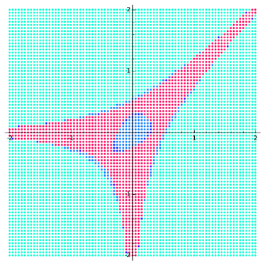
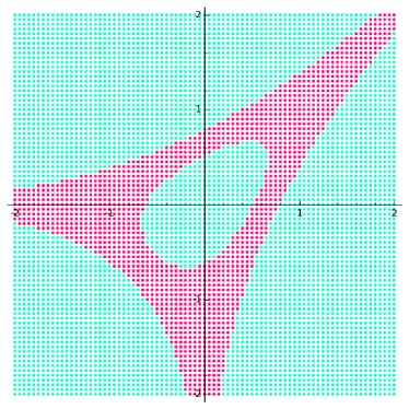
Figure 1. Plot of the amoeba of the polynomial $f(z_{1},z_{2})=z_{1}^{3}+z_{2}^{3}+b\cdot z_{1}z_{2}+1$ for $b=2$ and $b=-4$ on a $[-2,2]^{2}$ grid with $81\times 81$ grid points and relaxation level at most $4$. On the left hand side the turquoise points are the complement of the lopsided amoeba of $f$, light blue points are lopsided on relaxation level $3$ and dark blue points (very few; mainly at the boundary of hole in the middle) at relaxation level $4$. Red points were never lopsided and hence are presumed to belong to the amoeba of $f$. On the right hand side the amoeba coincides with the lopsided amoeba in this plot.

For every point ${\mathbf{w}}$ on the grid, we need to evaluate every monomial of $f$ or ${\rm CycRes}(f;r)$ at ${\operatorname{Log}}^{-1}({\mathbf{w}})=(\exp(w_{1}),\ldots,\exp(w_{n}))$. We test all points in our list for lopsidedness using $f={\rm CycRes}(f;2^{0})$ and ${\rm CycRes}(f;2^{1}),\ldots,{\rm CycRes}(f;2^{k})$; here $k=4$ . The algorithm successively searches for lopsidedness certificates for ${\mathbf{w}}\notin{\mathscr{L}}({\rm CycRes}(f;j))$ for $j\in\{0,\ldots,k\}$. If a certificate is found, then we save the level $j$. Otherwise $j$ is increased by $1$. If ${\rm CycRes}(f;r)$ is not lopsided at ${\mathbf{w}}$, then we presume that ${\mathbf{w}}\in\mathbb{R}^{n}$ is a point in ${\mathscr{A}}(f)$ since no certificate was found. This does not preclude further testing being performed, that may eliminate some of these points at a higher level.

7.4. Approximating Unlog Amoebas using Semi-algebraic Sets

In this last section we demonstrate how to use our software to obtain an approximation of the unlog amoeba ${\mathscr{U}}(f)$ for a given $f\in\mathbb{C}[\mathbf{z}^{\pm 1}]$ using semi-algebraic sets. Moreover, we can draw an implicit plot of (the boundary of) the image of this semi-algebraic description.

Returning to our running example (7.1) we compute the semi-algebraic description of ${\mathscr{U}}(f)$ in Singular. In this example, we use levels $1,2$, and $3$ given by the first three non-trivial instances of quickcyclicresultant for $f$. The output is shown in Figure 2. An interesting observation is that, according to this plot, the approximation of the sought semi-algebraic description of ${\mathscr{U}}(f)$ does not necessarily improve monotonically. One can see that there exist certain areas where the level $2$ approximation is better than the level $3$ approximation. This behavior does not seem to be a plotting artifact, and raises theoretical questions on the nature of the convergence of this approximation.

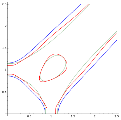
Figure 2. A plot of the semi-algebraic approximation of the unlog amoeba ${\mathscr{U}}(f)$ for $f(z_{1},z_{2})=z_{1}^{3}+z_{2}^{3}+2\cdot z_{1}z_{2}+1$ using relaxed polynomials given by quickcyclicresultant on level 1 (blue), 2 (dark green), and 3 (red).

References

- [AKNR13] M. Avendaño, R. Kogan, M. Nisse, and J. M. Rojas, Metric estimates and membership complexity for archimedean amoebae and tropical hypersurfaces, 2013, Preprint, arXiv:1307.3681.
- [BKS16] D.V. Bogdanov, A.A. Kytmanov, and T.M. Sadykov, Algorithmic computation of polynomial amoebas, Computer algebra in scientific computing, Lecture Notes in Comput. Sci., vol. 9890, Springer, Cham, 2016, pp. 87–100.
- [BPR03] S. Basu, R. Pollack, and M-F. Roy, Algorithms in Real Algebraic Geometry, Algorithms and Computations in Mathematics, vol. 10, Springer-Verlag Berlin Heidelberg, 2003.
- [CT65] J.W. Cooley and J.W. Tukey, An algorithm for the machine calculation of complex Fourier series, Math. Comp. 19 (1965), 297–301.
- [Dev16] The Sage Developers, Sagemath, the Sage Mathematics Software System (Version 6.4.1), 2016, http://www.sagemath.org.
- [DGPS15] W. Decker, G.-M. Greuel, G. Pfister, and H. Schönemann, Singular 4-0-2 — A computer algebra system for polynomial computations, http://www.singular.uni-kl.de, 2015.
- [dW17] T. de Wolff, Amoebas and their tropicalizations - a survey, to appear in: Analysis Meets Geometry: A Tribute to Mikael Passare, 2017.
- [FPT00] M. Forsberg, M. Passare, and A. Tsikh, Laurent determinants and arrangements of hyperplane amoebas, Adv. Math. 151 (2000), 45–70.
- [GKZ94] I.M. Gelfand, M.M. Kapranov, and A.V. Zelevinsky, Discriminants, resultants and multidimensional determinants, Birkhäuser, 1994.
- [Hil05] C.J. Hillar, Cyclic resultants, J. Symbolic Comput. 39 (2005), no. 6, 653–669.
- [HL07] C.J. Hillar and L. Levine, Polynomial recurrences and cyclic resultants, Proc. Amer. Math. Soc. 135 (2007), no. 6, 1607–1618 (electronic).
- [IdW16] S. Iliman and T. de Wolff, Amoebas, nonnegative polynomials and sums of squares supported on circuits, Res. Math. Sci. 3 (2016), 3:9.
- [Mik00] G. Mikhalkin, Real algebraic curves, the moment map and amoebas, Ann. of Math. (2) 151 (2000), no. 1, 309–326.
- [Mik04] by same author, Amoebas of algebraic varieties and tropical geometry, Different Faces of Geometry (S. K. Donaldson, Y. Eliashberg, and M. Gromov, eds.), Kluwer, New York, 2004, pp. 257–300.
- [Pel81] A. E. Pellet, Sur un mode de séparation des racines des équations et la formule de Lagrange, Darboux Bull. (2) 5 (1881), 393–395, In French.
- [PPT13] M. Passare, D. Pochekutov, and A. Tskih, Amoebas of complex hypersurfaces in statistical thermodynamics, Math. Phys. Anal. Geom. 16 (2013), no. 1, 89–108.
- [PR04] M. Passare and H. Rullgård, Amoebas, Monge-Ampère measures and triangulations of the Newton polytope, Duke Math. J. 121 (2004), no. 3, 481–507.
- [PT05] M. Passare and A. Tsikh, Amoebas: their spines and their contours, Idempotent mathematics and mathematical physics, Contemp. Math., vol. 377, Amer. Math. Soc., 2005, pp. 275–288.
- [Pur08] K. Purbhoo, A Nullstellensatz for amoebas, Duke Math. J. 14 (2008), no. 3, 407–445.
- [Rul03] H. Rullgård, Topics in geometry, analysis and inverse problems, Ph.D. thesis, Stockholm University, 2003.
- [SdW13] F. Schroeter and T. de Wolff, The boundary of amoebas, 2013, Preprint, arXiv:1310.7363.
- [TdW15] T. Theobald and T. de Wolff, Approximating amoebas and coamoebas by sums of squares, Math. Comp. 84 (2015), no. 291, 455–473.
- [The02] T. Theobald, Computing amoebas, Experiment. Math. 11 (2002), no. 4, 513–526 (2003).