ON THE METALLICITY DISTRIBUTION OF THE PECULIAR GLOBULAR CLUSTER M22
Abstract
In our previous study, we showed that the peculiar globular cluster (GC) M22 contains two distinct stellar populations, namely the - and - groups with different physical properties, having different chemical compositions, spatial distributions and kinematics. We proposed that M22 is most likely formed via a merger of two GCs with heterogeneous metallicities in a dwarf galaxy environment and accreted later to our Galaxy. In their recent study, Mucciarelli et al. claimed that M22 is a normal mono-metallic globular cluster without any perceptible metallicity spread among the two groups of stars, which challenges our results and those of others. We devise new strategies for the local thermodynamic equilibrium (LTE) abundance analysis of red giant branch (RGB) stars in GCs and show there exists a spread in the iron abundance distribution in M22.
1 INTRODUCTION
During the last decade, there has been a dramatic paradigm shift on the the definition of the GC systems. Despite the formerly accepted idea of chemical homogeneity, the variations in the lighter elemental abundances in several GCs in our Galaxy had been known for several decades. The Lick-Texas Group is one of those who undertook the systematic study of lighter elemental abundances in several GCs in our Galaxy since 1990’s (e.g. Sneden et al., 1991; Kraft, 1994). Thanks to the advent of high performance multi-object high-resolution spectrographs mounted on the large aperture telescopes, it is now possible for us to look into the detailed substructure of elemental abundance distributions of the Milky Way GC systems (e.g. Carretta et al., 2009a). The decades-long lighter elemental variation issue in GC stars is now considered to be a generic feature of normal GCs in our Galaxy, most likely engraved during the multi-phase normal GC formation (e.g. D’Antona & Ventura, 2007; Decressin et al., 2007; D’ercole et al., 2008).
Contrary to the normal GC system, one of the key features of the peculiar GCs, such as Cen, is the spread or the distinctive substructure in the metallicity distributions (e.g. Lee et al., 1999; Johnson & Pilachowski, 2010), where the heavy elements must have been supplied by supernovae (SNe). To retain ejecta from energetic SNe explosions, such peculiar GC systems must have been much more massive in the past and they are generally thought to be the remaining core of a disrupted dwarf galaxy and accreted to our Galaxy later in time, expected from the hierarchical merging paradigm in the CMD cosmological model (e.g. Searle & Zinn, 1978; Freeman, 1993; Moore et al., 1999). The existence of these peculiar GCs have major implications in the context of near field cosmology (e.g. Bland-Hawthorn& Freeman, 2014); Are they one of the original building blocks to our Galaxy, mitigating so-called the “missing satellite problem?” (Moore et al., 1999); How did they relate to the formation of the Galactic halo and numerous streamers? (e.g. Belokurov et al., 2006). These are examples of the outstanding problems that we have to challenge in the next decade.
To measure metallicity of stars in GCs from high-resolution spectroscopy, the LTE (local thermodynamic equilibrium) analysis is being widely used for the sake of convenience, where the final results critically depend on the stellar atmosphere models with a few appropriate input stellar parameters, such as effective temperature, surface gravity and turbulent velocity, and the oscillator strengths of the absorption lines. Although simple, the derivation of stellar elemental abundances is not a trivial task even for nearby bright stars. The recent study of Baines et al. (2010) may highlight the current situation. They showed that the interferometric effective temperatures for nearby K giant stars do not agree with those from spectroscopic observations, suggesting a missing source of opacities in stellar atmosphere models. The situation would be even worse for fainter stars, such as those in GCs. Another line of difficulty is that changes in surface gravity can mimic the chemical compositions in the regime of RGB stars in GCs (for example, see Gray, 2008), where H- is the major source of the continuum opacity and the H- population varies with the electron pressure, therefore, the surface gravity of RGB stars.
The spread in the metallicity distribution of M22 has been a controversial topic for many years. The recent several studies of the cluster have found that M22 has a bimodal heavy elemental abundance distribution (e.g., Da Costa et al., 2009; Lee et al., 2009a; Lee, 2015; Marino et al., 2009, 2011, 2012, 2013). The high-resolution spectroscopic elemental abundance measurements of RGB stars in the peculiar GC M22 by Brown & Wallerstein (1992)111See also Figure 3 of Lee et al. (2009a), where we showed a bimodal heavy elemental abundance distribution including iron of M22 RGB stars using the results of Brown & Wallerstein (1992). and Marino et al. (2009, 2011) showed a distinctive bimodal metallicity distribution. Their results were based on the spectroscopic and , which require the excitation and ionization equilibria,
and
where and are iron abundances from Fe I and Fe II lines and is the excitation potential.
It has been frequently suspected that the iron abundance from the Fe I line suffers from non LTE (NLTE) effects (see, for example, Thévenin & Idiart, 1999; Kraft & Ivans, 2003; Lee et al., 2005, 2006; Lee, 2010). Since metal-poor stars have much weaker metal absorption in the ultraviolet, more non-local ultraviolet flux can penetrate from the deeper layers. This flux is vital in determining the ionization equilibrium of the atoms, resulting in deviations from LTE (Thévenin & Idiart, 1999; Kraft & Ivans, 2003; Lee et al., 2005). In this regard, the traditional spectroscopic surface gravity determination method may be in error, which led Kraft & Ivans (2003) to propose to use the photometric gravity for elemental abundance study of RGB stars in GCs, where the bolometric correction could be the dominant source of uncertainty for the photometric gravity. In principle, the use of the [Fe/H]II abundance as for the metallicity scale of RGB stars in GCs is most likely an appropriate approach since Fe II is by far the dominant species and, therefore, the number of Fe II atoms is unaffected by the NLTE effect. In practice, however, the [Fe/H]II abundances of RGB stars sensitively depends not only on the surface gravity and effective temperature but also on the metallicity of the input atmosphere model, which also affects the continuum opacity. We will show later that an iterative procedure is useful to reduce the error raised by the incorrect metallicity of the input atmosphere model.
In their recent study, Mucciarelli et al. (2015, Mu15 hereafter) re-analyzed M22 RGB stars of Marino et al. (2011) using three different approaches: (1) Spectroscopic and (Method 1); (2) spectroscopic and photometric (Method 2); and (3) photometric and (Method 3). They confirmed a bimodal iron abundance distribution of M22 RGB stars by Marino et al. (2009, 2011), when they relied on spectroscopic and (Method 1). Oddly enough, when they used photometric (Method 2 and 3 by Mu15), the allegedly well-established bimodal iron distribution of M22 disappeared in [Fe/H]II. Using the photometric gravity is most likely a correct approach but how can this be interpreted? We will show later that it is likely that Mu15 used incorrect surface gravity and the metallicity of input atmosphere models in their analysis and the separation in [Fe/H]II can be brought out more fully if different methods to compute these parameters are used.
In this paper, we revisit the internal metallicity distribution of M22. We developed new methods to estimate the surface gravity and we found that there exists substantial metallicity difference between the - and - groups222The - (calcium-weak) and the - (calcium-strong) groups are defined to be RGB stars with smaller or larger index values, respectively, at a given magnitude. They are equivalent to the -process-poor (-) and the -process-rich (-) groups classified by Marino et al. (2011). in M22 (Lee et al., 2009a; Lee, 2015). Throughout this paper, metallicity refers to [Fe/H]II, unless specified.
2 LESSONS LEARNED FROM PREVIOUS STUDIES
Before turning to the metallicity distribution of M22, we would like to revisit the critical issues on the LTE analysis; surface gravity, effective temperature and the metallicity of the input atmosphere model.
2.1 [Fe/H]II with surface gravities independent of ionization equilibrium
As mentioned above, Kraft & Ivans (2003) suggested to use [Fe/H]II derived from photometric gravity as metallicity of RGB stars. They pointed out that [Fe/H]II is essentially independent of NLTE effects, such as Fe I overionization by non-local UV flux since Fe II is the dominant species in GC RGB stars.
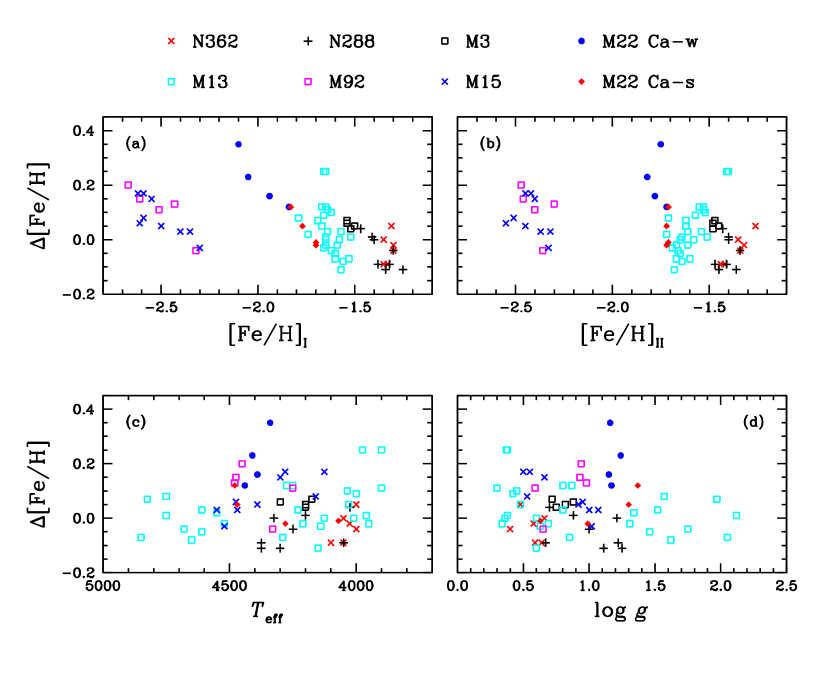
In Figure 1, we show plots of [Fe/H] against [Fe/H]I, [Fe/H]II, and for the six Group 1 clusters333Clusters with and based on colors and absolute magnitudes. of Kraft & Ivans (2003). Of particular concern is Figure 1 (a) and (b), where each GC is showing its own correlation between [Fe/H]I versus [Fe/H] (or [Fe/H]II versus [Fe/H]).
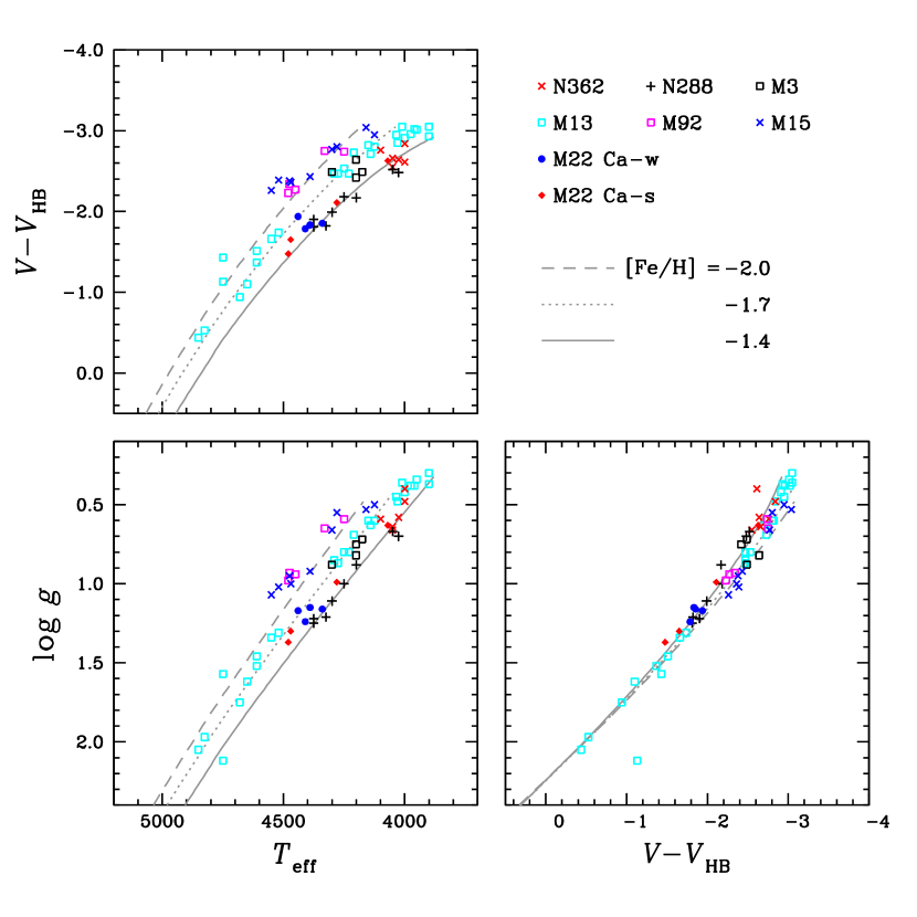
In Figure 2, we show plots of versus , versus , and versus for the six Group 1 GCs. Also shown are Victoria-Regina model isochrones for 12 Gyr (VandenBerg et al., 2006). To estimate the level of the model isochrones, we used our previous relation (Lee et al., 2014),
| (1) |
Note that this metallicity-luminosity relation for RR Lyrae variables gives = 18.54 0.13 mag for LMC. It also should be emphasized that the adopted age of the model isochrones does not affect our results presented in this work.
In plots of versus and versus , the loci of the model isochrones are in excellent agreement with the observations. It should not be a surprise that, at a given temperature, the surface gravity of the metal-poor stars is lower and is smaller than those of the metal-rich stars. This implies that applying a single versus relation for groups of stars with heterogeneous metallicity may result in incorrect surface gravity estimates and, as a consequence, incorrect elemental abundances. This is especially true when one adopt [Fe/H]II as metallicity of GC RGB stars. The Fe II line opacity does not vary with surface gravity since the almost all iron atoms are populated in the first ionized level. On the other hand, the H- continuum opacity is sensitively dependent on the electron pressure and, therefore, surface gravity. As a consequence, in the regime of the linear part of the curve of growth, at fixed metallicity, the equivalent widths (EWs) of Fe II lines increases with decreasing surface gravity. In the figure, the surface gravity dependency on the metallicity of the metal-poor RGB stars at a fixed temperature is given by
| (2) |
In other words, a change in the surface gravity by 0.1 in the cgs unit corresponds to a change in metallicity by about 0.2 dex in the figure.
On the other hand, a rather tight relation in versus can be found, suggesting that the magnitude can be a reddening- and distance-independent surface gravity indicator for RGB stars in GCs. (see also, Lee et al., 2004, for the use of as a temperature indicator of heavily reddened metal-rich GC Palomar 6). But caution is advised that the observed magnitude can be vulnerable to the foreground differential reddening effect.
2.2 The utility of spectroscopic effective temperature
As mentioned previously, Kraft & Ivans (2003) suggested to use the photometric surface gravity. However, ironically, under the condition that LTE is not valid, they concluded to use spectroscopic temperature from Fe I lines. We would like to discuss the utility of the spectroscopic effective temperature under the assumption that the conclusion made by Kraft & Ivans (2003) is valid.
In Figure 3, we show plots of the against the excitation potential for NGC 6752-mg10 by Yong et al. (2013). As they noted, the quality of their spectra is superb; a resolving power of = 110,000 and S/N 150 per pixel near 5140 Å. To perform a LTE abundance analysis, we used the 2014 version of the stellar line analysis program MOOG (Sneden, 1973) and we interpolated -enhanced Kurucz atmosphere models with new opacity distribution functions using a FORTRAN program kindly provided by Dr. McWilliam (2005, private communication). Using the weak Fe I lines, ) , we derived a spectroscopic temperature for this star by forcing the condition of the excitation equilibrium, i.e. / = 0, and we obtained the effective temperature of 4275 K. Note that our effective temperature for this star is slightly cooler than those from the line-by-line differential analysis with respect to NGC 6752-mg9 and NGC 6752-mg6 by Yong et al. (2013), 4291 K and 4295 K, respectively. We derived the linear fits to the data, assuming slope, and we show them with thin dashed lines in the figure. In the parentheses in each panel, we also show the value in the cgs unit, the slope in the excitation potential versus the iron abundance, [Fe/H]I and [Fe/H]II. As can be seen, once the spectroscopic effective temperature is correctly determined, the assumption of the excitation equilibrium holds for rather wide range of the surface gravity, 1.20 in this case. Therefore, it can be concluded that the slightly incorrect input surface gravity does not significantly affect the spectroscopic effective temperature in our results presented here.
2.3 Iterative derivation of metallicity: [Fe/H]I and [Fe/H]II versus input atmosphere model parameters
It is well-known fact that the inferred metallicity of GC RGB stars from high resolution spectroscopy is critically dependent on the stellar parameters of the input atmosphere model. Here, we show how [Fe/H]I and [Fe/H]II behave against the changes in the input stellar parameters. We also would like to demonstrate the importance of the iterative derivation of the metallicity.
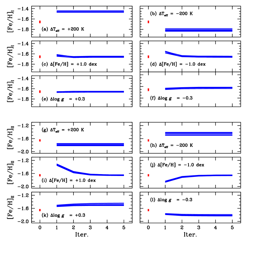
In Figure 4, we show [Fe/H]I and [Fe/H]II of 9 RGB stars in NGC 6752 by Yong et al. (2013). In each panel, the red crosses denote our spectroscopic [Fe/H]I and [Fe/H]II which were derived using the weak Fe I and Fe II lines measured by Yong et al. (2013). It should be noted that our [Fe/H] values are consistent with those of Yong et al. (2013). Using our spectroscopic , , and [Fe/H] as reference grids, we examine how the changes in the stellar parameters of the input atmosphere models affect the resultant metallicity. We run MOOG using the Kurucz atmosphere models, whose stellar parameters are different from the reference grids by = 200 K, [Fe/H] = 1.0, and = 0.3. We use the [Fe/H]II abundances returned from MOOG as the reference metallicity and we calculate new atmosphere models, with which we run MOOG again. We iterate this process five times and we show our results in Figure 4 with blue solid lines.
The figure shows that the inferred [Fe/H]I abundances with sufficient numbers of iterations are only affected by the changes in the effective temperature. As shown, [Fe/H]I abundances of individual stars against the changes in the metallicity and the surface gravity of the input model atmosphere converge to their spectroscopic [Fe/H]I values within 2 or 3 iterations. However, the iterations with the effective temperature offsets of 200K fail to regain spectroscopic [Fe/H]I, implying incorrect estimate results in irrecoverable deviations in the derived metallicity.
The [Fe/H]II behaves differently against the changes in input stellar parameters. The inferred [Fe/H]II abundances with the effective temperature offsets shifted in the opposite direction of the changes in the [Fe/H]I abundance. A rather simple explanation of the temperature effect in cool stars can be found in Gray (2008), for example. Similar to [Fe/H]I, the spectroscopic metallicity can be regained with the iterative derivation of the [Fe/H]II abundances against the changes in the metallicity of the input atmosphere model but, however, the difference in [Fe/H]II between the spectroscopic metallicity and that from the first iteration is much larger than that can be seen in [Fe/H]I. As we have already discussed earlier, the [Fe/H]II abundance sensitively depends on the surface gravity of the input atmosphere model. The Figure shows that the spectroscopic metallicity can not be regained with incorrect surface gravity.
We also performed the same procedures using the [Fe/H]I abundances of individual stars as reference metallicity to calculate the input atmosphere model used in the next iteration and we obtained the same results shown above.
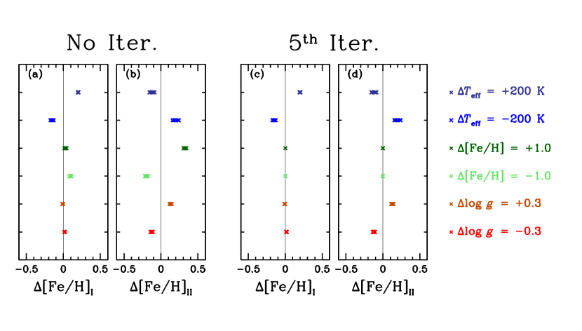
Figure 5 summarize our exercise. For both [Fe/H]I and [Fe/H]II, the inferred metallicity from the first iteration with offsets in the stellar parameters could be very different from those with correct stellar parameters. However, some discrepancies vanish after 2 or 3 iteration processes.
Our exercise demonstrates that, with the iterative procedure, the [Fe/H]I abundance depends only on the effective temperature, while the [Fe/H]II abundance depends both on the effective temperature and the surface gravity. It also shows the importance of having correct stellar parameters, especially for the LTE analysis of [Fe/H]II abundances, as we have discussed earlier.
3 PREVIOUS EVIDENCE OF THE BIMODAL METALLICITY DISTRIBUTION OF M22
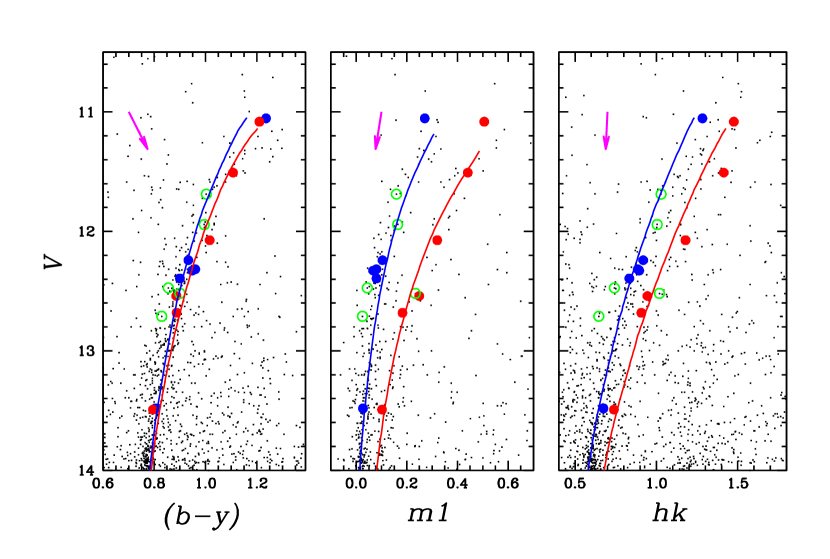
The vivid evidence of the bimodal metallicity distribution of RGB stars in M22 from narrow-band photometry and high-resolution spectroscopy can be found in Lee et al. (2009a), Lee (2015) and Marino et al. (2009, 2011). In our earlier study of the cluster, we extensively discussed that there are several observational lines of evidence that cannot be easily explained without invoking a bimodal metallicity distribution between two groups of stars, namely the - and the - groups as shown in Figure 6 (e.g., see Figures 9, 13 – 21 of Lee, 2015, and references therein);
- •
-
•
The infrared Ca II triplet by Da Costa et al. (2009) also show a bimodal distribution among RGB stars in M22.
-
•
The versus CMD as shown in Figure 6 (see also Figure 19 of Marino et al., 2011) also requires a bimodal metallicity distribution in M22 RGB stars. The variation in the lighter elements only, such as CNO, cannot explain this distinct double RGB sequences of M22. The differential foreground reddening effect cannot reproduce the observed multi-color CMDs accordingly (Lee, 2015).
-
•
The magnitude of the RGB bump, , of the - group is significantly fainter than that of the - group, which strongly suggests that the - group is more metal-rich than the - group is. The difference in the between the two groups cannot be explained by the differential foreground reddening effect (Lee, 2015).
-
•
The slope of the - RGB stars in the versus CMD is significantly larger than that of the - RGB stars, indicative of the metal-rich nature of the - group (Lee, 2015).
- •
-
•
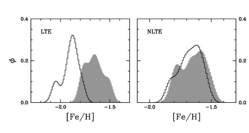
Finally, another piece of evidence can be found in the metallicity distribution of the blue horizontal branch (BHB) stars in M22 (Marino et al., 2013). In Figure 7, we show the metallicity distributions for M22 BHB stars. Both the LTE and the NLTE treatments show the similar degree of metallicity spreads in [Fe/H]I and [Fe/H]II (six stars for [Fe/H]I and seven stars for [Fe/H]II). As shown in Table 3 of Marino et al. (2013), their derived [Fe/H]II value is less sensitive to the effective temperature and to the surface gravity, [Fe/H]II= 0.06 dex and 0.01 dex for = 170 K and = 0.20 respectively, and we are likely seeing the real metallicity spread in M22 BHB stars.
4 NO METALLICITY SPREAD IN M22?
As mentioned above, Mu15 re-analyzed M22 RGB stars of Marino et al. (2011) using three different approaches. We show 17 RGB and asymptotic giant branch (AGB) stars studied by Mu15 in Figure 6. Among 12 RGB stars tagged by Mu15, six RGB stars belong to each of two RGB groups, according to our previous classification of RGB stars based on the index at a given magnitude.
Figure 8 shows a plot of the versus of spectroscopic target stars, where the filled symbols are for Method 1 (spectroscopic and ) and the open symbols are for Method 2 (spectroscopic and photometric ) of Mu15. Also shown are Victoria-Regina model isochrones for 12 Gyr with [Fe/H] = 1.40, 1.70 and 2.00 dex (VandenBerg et al., 2006). The most conspicuous feature of the figure is that the positions of stars from Method 2 by Mu15 are rather well aligned in a narrow strip between model isochrones with [Fe/H] = 1.40 and 1.70 dex on the – plane, which is most likely due to the adopted single – relation by Mu15. It should be worth to point out that, because the CMD of Mu15 has a single RGB sequence, their photometric effective temperature and surface gravity will also define a single isochrone. The broad band colors adopted by them are not sensitive to small [Fe/H] differences. On the other hand, positions of stars from Method 1 occupy rather wide ranges in surface gravity at given effective temperature.
We performed a LTE abundance analysis using EWs of M22 RGB stars measured by Mu15 to calculate the the mean iron abundance dependence on model atmospheres. In Table 1, we show our result for eight RGB stars in M22 with 0.5 1.5, where is the photometric surface gravity in the cgs unit. As shown in the table, the change in the surface gravity by 0.2 results in [Fe/H]II 0.1 dex at the fixed , in the sense that the [Fe/H]II value increases with the surface gravity.444Note that the metallicity dependency on the surface gravity from the LTE analysis is about four times smaller than that from the isochrones as in Equation 2. If we take this at face value, a single – relation, which is valid only for mono-metallic stellar systems such as normal GCs in our Galaxy, may be responsible for the narrow uni-modal [Fe/H]II distribution of M22 RGB stars as claimed by Mu15 as shown in their Figure 2.
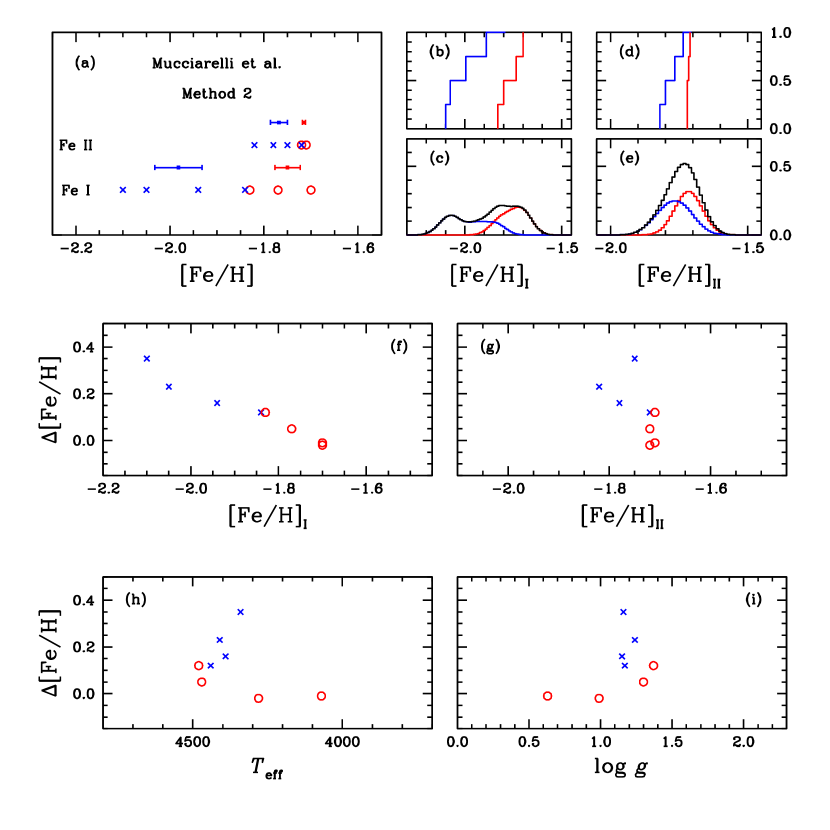
In Figure 9, we show the metallicity distribution of M22 RGB stars using Table 4 of Mu15 (Method 2). Note again that we use 8 RGB stars with 0.5 1.5 only (corresponding to 11.5 12.75 mag in Figure 6) to avoid the potential effect raised by very different surface gravity in the stellar atmosphere model calculations. According to our population classification scheme for M22 based on our index at a given magnitude, stars 61, 71, 200068 and 200076 belong to the - group, while stars 51, 88, 200025 and 200101 belong to the - group. Figure 9 (a) shows that each RGB group has different mean iron abundance both in [Fe/H]I and [Fe/H]II. It is very interesting to note that the differences in the mean iron abundances between the two groups are larger than a 2.5 level both in [Fe/H]I and [Fe/H]II, although the separation in the mean [Fe/H]II values is as small as 0.05 dex. In Table 2, we show our results (Mu15 M2).
Figure 9 (b) – (e) show the cumulative metallicity distributions and the generalized histograms of the metallicity distributions for each group. As shown, the [Fe/H]I distribution show two distinct peaks, while that for [Fe/H]II shows a broad single peak in the overall metallicity distribution, similar to those obtained by Mu15. But it should be emphasized that the [Fe/H]II distribution by Mu15 is composed of two separate mono-metallic distributions; only the mean [Fe/H]II values from the Method 2 by Mu15 for each group of stars happen to be similar. We performed a Student’s -test to see if the metallicity distributions of the two groups of stars are identical. We obtained that the significance levels to reject the hypothesis that the mean [Fe/H] values of the - and the - groups are identical, are 1.93 % and 8.98 % for [Fe/H]I and [Fe/H]II, respectively. We also performed a randomization test. The significance levels to reject the hypothesis for being an identical metallicity distribution from bootstrap method are 0.00 % for both [Fe/H]I and [Fe/H]II, strongly suggest that the metallicity distributions for the - and the - groups by Mu15 are not statistically identical. It should not be a surprise because Lee (2015) already discussed many aspects of heterogeneous nature between the two groups as summarized in §3.
Figure 9 (f – g) shows [Fe/H] (= [Fe/H]II [Fe/H]I) against [Fe/H]I and [Fe/H]II and they are very intriguing. It should be reminded that we chose stars with a narrow range of magnitude for both groups to avoid the potential effect raised by the very different surface gravity. As shown in the figure, the discrepancies between [Fe/H]I and [Fe/H]II of the - group RGB stars are preferentially much greater than those of the - group, reaching as large as [Fe/H] 0.4 dex. For comparison, we show [Fe/H] of M22 along with six group 1 GCs by Kraft & Ivans (2003) in Figure 1, where the much greater [Fe/H] values of the - RGB stars in M22 can be clearly seen. If the two groups of stars have the same metallicity and the same surface gravity so that they suffer similar degree of NLTE effect, one would expect to see the similar degree of [Fe/H] for both groups, in sharp contrast to the results of Method 2 by Mu15. We will show later that, with a mock peculiar GC, the incorrect surface gravity estimate by Mu15 and the incorrect metallicity of input model atmospheres are responsible for the discrepancy in [Fe/H].
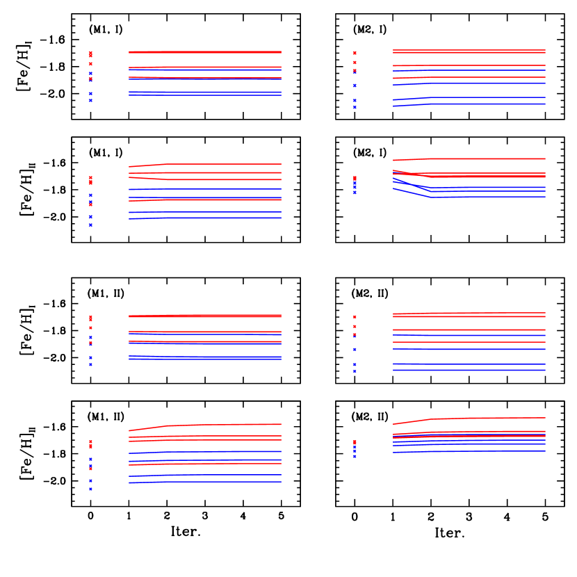
Another aspect needs to consider is the initial metallicity used during the atmosphere model calculations. In Figure 10, we show plots for eight M22 RGB stars, similar to Figure 4 for NGC 6752. In parentheses of each panel, we show the method for the metallicity derivation by Mu15 (M1 or M2) and the reference metallicity for the iterations (I for [Fe/H]I and II for [Fe/H]II). In the figure, the crosses denote the Mu15’s [Fe/H]I and [Fe/H]II values from M1 and M2 methods and blue and red colors denote the - and - RGB stars, respectively. Using [Fe/H]I and [Fe/H]II abundances as trial metallicities and and from M1 and M2 methods by Mu15, we performed the iterative derivations of [Fe/H]I and [Fe/H]II for individual stars. As shown, [Fe/H]I values do not vary significantly with the number of iterations with respect to the spectroscopic [Fe/H], meaning that the effective temperature adopted by Mu15 is correct. On the other hand, the discrepancy in [Fe/H]II for - RGB stars from Method 2 are preferentially larger, indicating that the surface gravities of the - RGB stars adopted by Mu15 is most likely underestimated. The figure also indicates that the separation in the [Fe/H]II abundances between the - and the - groups becomes larger with the iteration processes.
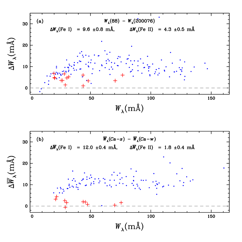
Finally, comparisons of EWs between the two groups may also help to elucidate the underlying metallicity distributions of the cluster. In Figure 11(a), we show the line-by-line EW difference between stars 88 (-) and 200076 (-). Both stars have similar visual magnitudes and colors, (, ) = (12.54, 0.89) for the star 88 and (12,39, 0.90) for the star 200076. Therefore, if there is no significant foreground differential reddening and if the both stars have the same metallicity, they should have similar , and furthermore the similar EW strengths. As shown in the figure, the EWs of the - group star 88 are systematically larger than those of the - group stars 200076. A comparison between the mean EWs of the four - group stars (51, 88, 200025 and 200101) and the four - group stars (61, 71, 200068 and 200076) show the same trend that the mean EWs of the - group are larger than those of the - group, 12.0 0.4 mÅ for Fe I lines and 1.8 0.4 mÅ for Fe II lines. Note that the eight stars above have similar visual magnitudes and colors and they should have similar , and [Fe/H] if they belong to a single stellar population. A simple explanation why Fe II lines are less sensitive to changes in metallicity as follows. Since both the fraction of Fe I atoms and the H- continuum opacity of RGB stars depend on the electron pressure (i.e., metallicity or surface gravity) and, furthermore, the two effects are expected to cancel out, the EWs of Fe I lines grow with metallicity at fixed effective temperature. On the other hand, the Fe II atoms are the dominant species and only the electron pressure has an effect on the H- continuum opacity, which has an opposite effect on the growth of EWs with metallicity. Therefore, the EWs of Fe II lines grows at a slower rate.
We suspect that the metallicity measurements by Mu15 may be slightly incorrect and we devise new methods to derive metallicity of RGB stars in appropriate and consistent manners.
5 M55 + NGC 6752: A MOCK PECULIAR GC
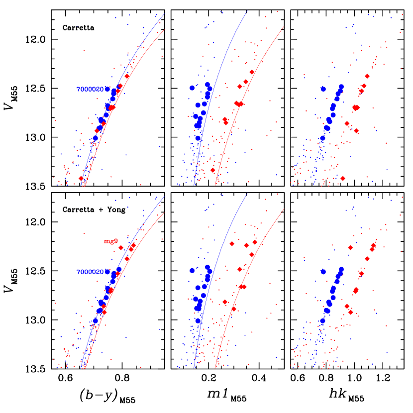
In our previous study, Lee (2015) showed that a combination of two normal GCs, M55 and NGC 6752, can reproduce many aspects of peculiar photometric characteristics of M22. In Figure 12, we show a composite CMDs for M55 and NGC 6752, which may highlight the importance of the choice of photometric passbands to distinguish multiple stellar populations in GCs. For NGC 6752 stars, we add offsets of 0.030, 0.010, 0.005, and 0.700 mag in (), , ,555We adopt the interstellar reddening law by Anthony-Twarog et al. (1995); , , and . and , respectively, in order to place NGC 6752 stars in the M55 colors and magnitude scale. In the figure, we also show RGB stars studied from high-resolution spectroscopy of the clusters (Carretta et al., 2009b; Yong et al., 2013)666 It should be mentioned that the spectral resolving power for the data from Yong et al. (2013) is much higher than that of Carretta et al. (2009b), 110,000 versus 40,000, and the scatter in the mean metallicity for NGC 6752 by Yong et al. (2013) is much smaller than that by Carretta et al. (2009b). Note that M55-7000020 (Carretta et al., 2009b) and NGC 6752-mg9 (Yong et al., 2013) are most likely AGB stars of the clusters, and we do not make use of them in the following analysis. and the Victoria-Regina model isochrones for 12 Gyr with [Fe/H] = 1.84 and 1.53.
Despite the difference in metallicity, the RGB sequence of NGC 6752 is in excellent agreement with that of M55 in versus CMDs, and it is difficult to discern different populations. In such a case, one can be easily misled to adopt a single – relation for heterogeneous stellar populations. On the other hand, the distinct double RGB sequences can be clearly seen in versus and versus CMDs, where the necessity for double – relations is obvious.
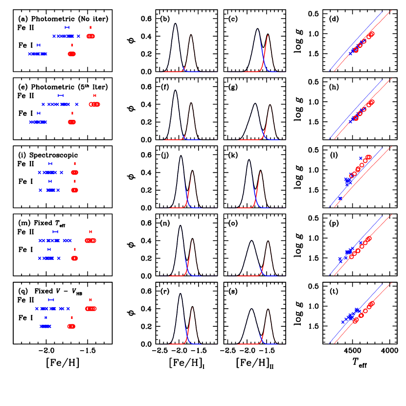
5.1 Photometric method using two separate relations
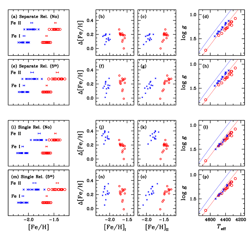
First, we derived the metallicity distributions of M55 and NGC 6752 by employing two separate – relations, following the procedure recommended by Kraft & Ivans (2003). With the EW measurements by Carretta et al. (2009b) for Fe I and Fe II lines, we performed a LTE abundance analysis. Applying the color-temperature relation and the equation for the bolometric correction given by Alonso et al. (1999), we calculated the photometric effective temperature and the surface gravity using our own Strömgren photometry. During our calculations, we adopted [Fe/H] = 1.95 and 1.55 as the input metallicities for M55 and NGC 6752, respectively (Carretta et al., 2009b), and we used the distance moduli and foreground reddening values by Harris (1996). During our analysis, we used weak lines only, ) , for both Fe I and Fe II in order to minimize the effect of the adopted micro-turbulent velocity on the derived metallicity. We show our results in Table 3 and Figure 13. Our [Fe/H]II measurements for the clusters are in good agreement with those by Carretta et al. (2009b), [Fe/H]II = 0.01 0.03 dex for M55 and [Fe/H]II = 0.05 0.02 dex for NGC 6752 in the sense of current work minus those of Carretta et al. (2009b). These small differences are thought to be mainly due to slightly different final color-temperature relations. Carretta et al. (2009b) used the color-temperature relations given by Alonso et al. (1999) to derive the initial but they applied their own versus magnitude relation to derive their final adopted .
In Figure 13 (b) and (c), we show [Fe/H] (= [Fe/H]II [Fe/H]I) against [Fe/H]I and [Fe/H]II, where the extent of [Fe/H] for both clusters are in good agreement with those of six GCs studied by Kraft & Ivans (2003) as shown in Figure 1.
Figure 13 (d) shows a plot of versus along with the Victoria-Regina model isochrones for 12 Gyr with [Fe/H] = 1.84 and 1.55 (VandenBerg et al., 2006). At a given , the stars in the metal-poor cluster M55 have lower surface gravity, although the mean difference in between M55 and NGC 6752 is not as large as that can be inferred from model isochrones. Using separate relations, the differences in the mean [Fe/H]I and [Fe/H]II are 0.44 0.02 and 0.47 0.03, respectively, and they are in excellent agreement.
Following the same procedure described earlier, we performed iterative derivations of [Fe/H]I and [Fe/H]II for the clusters. As shown in Figure 13 and Table 3, [Fe/H]I and [Fe/H]II from iterative processes are in good agreement with those without the iterative process.
We also make use of the EW measurements for the Fe I and Fe II lines for NGC 6752 RGB stars by Yong et al. (2013). We show our results in Figure 15 and Table 3. Note that the oscillator strengths for the individual lines are slightly different between those adopted by Carretta et al. (2009b) and Yong et al. (2013). For our results presented in Figure 15, we used the oscillator strengths by Yong et al. (2013) because they provided more lines. As summarized in Table 3, [Fe/H]I and [Fe/H]II abundances using -values by Carretta et al. (2009b) and Yong et al. (2013) are slightly different, but the differences in the mean values are no larger than 0.04 dex. Therefore, it can be said that the choice of the set of oscillator strengths does not affect our primary results presented here. The differences in [Fe/H]I ([Fe/H]I = [Fe/H]I [Fe/H]I,M55) and [Fe/H]II ([Fe/H]II = [Fe/H]II [Fe/H]II,M55) are 0.38 - 0.45 dex and 0.44 - 0.50 dex, respectively.
5.2 Photometric method using a single relation
Assuming that our mock GC (i.e. M55 + NGC 6752) is a mono-metallic GC with [Fe/H] dex (i.e. that of NGC 6752), we calculated photometric effective temperatures and surface gravities of individual stars using the color-temperature relation and the equation for the bolometric correction given by Alonso et al. (1999). Using the weak Fe I and Fe II lines only, ) , we derived the metallicity of individual stars in both clusters and we show our results in Table 3 and Figure 13. The mean [Fe/H]I abundance of M55 remains unchanged, while that of [Fe/H]II increases almost 0.15 dex compared to the results from correct input stellar parameters for M55 presented in §5.1. The difference in the effective temperature between the two methods (i.e. two separate relations versus a single relation for M55 and NGC 6752) is negligibly small, = 12 K, in the sense that the mean effective temperature of M55 RGB stars is slightly warmer when the correct color-temperature relation is used. As we have discussed earlier, the [Fe/H]I abundance is relatively insensitive to changes in the surface gravity and the metallicity of the input model atmosphere since the effects due to change in the number of Fe I species and that in H- continuum opacity are expected to cancel. However, the surface gravity becomes larger, 0.1, and the metallicity of the input model atmospheres is higher (from 1.95 to 1.55 dex) when a single relation with respect to NGC 6752 is used. Both effects greatly enhance the H- continuum opacity, while the fraction of Fe II to the total number of iron atoms is unaffected since Fe II is by far the dominant species. As a consequence, the mean [Fe/H]II abundance of M55 appears to be enhanced at given EWs.
In Figure 13 (l), we show a plot of versus with a single relation, where RGB stars in both clusters are aligned well on a single locus. Figure 13 (j) and (k) show [Fe/H] against [Fe/H]I and [Fe/H]II showing large discrepancies in M55 RGB stars, reminiscent of the M22 - stars from Method 2 of Mu15 as shown in Figure 9. The metallicity distributions of [Fe/H]I and [Fe/H]II from a single – relation shown in Figure 14 (b) and (c) are intriguing, since the two peaks in the [Fe/H]II distribution become less conspicuous with a single relation with respect to NGC 6752.
Our result with a mock GC strongly suggests that applying a single photometric relation in order to derive the effective temperatures and surface gravities of individual stars in peculiar GCs with heterogeneous metallicities and perhaps ages, such as M22, may result in slightly incorrect metallicity scales and distributions.
5.3 Spectroscopic method
We also performed a traditional analysis using the spectroscopic effective temperatures and the surface gravities, which requires the excitation and ionization equilibria of iron abundances. Our results are shown in Figures 14 (i – l) and 15 (i – l). As shown in Table 3, our mean spectroscopic [Fe/H] values are in good agreement with those of Carretta et al. (2009b) and Yong et al. (2013). The difference in metallicity between M55 and NGC 6752 is [Fe/H]II = 0.32 – 0.42 dex, depending on the data sets. It should be mentioned that our spectroscopic [Fe/H] value of NGC 6752 from Carretta et al. (2009b) is about 0.1 dex higher than that from Yong et al. (2013), which is consistent with the iron abundances of [Fe/H] = 1.56 dex (Carretta et al., 2009b) and 1.65 dex (Yong et al., 2013) for the cluster. The origin of this discrepancy of the mean metallicity of NGC 6752 is beyond the scope of this study and we decline to discuss this matter further.
5.4 Using the evolutionary with the spectroscopic
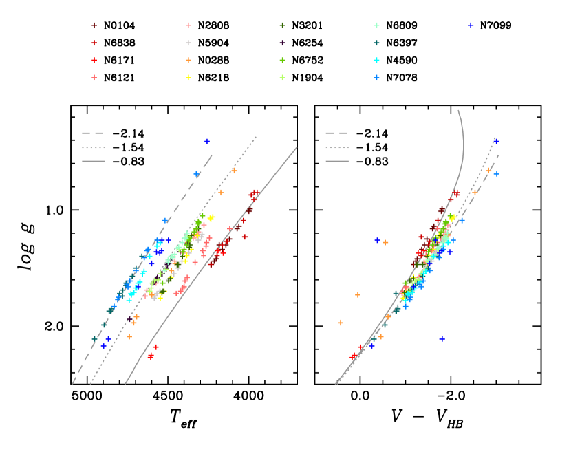
As shown in Figure 2, the model isochrones can provide a useful means to derive the stellar parameters. In Figure 16, we show the similar plots for 17 GCs from the homogeneous elemental abundance study by Carretta et al. (2009b). Also shown are the Victoria-Regina isochrones for the age of 12 Gyr and they appear to be in excellent agreement with observations.
We devise a new strategy to derive evolutionary surface gravities of RGB stars in GCs under the assumption that the excitation equilibrium of Fe I lines is applicable in such stellar atmospheres and, furthermore, excitation equilibrium holds for rather wide range of the surface gravity. As shown in Figure 2 and 16, at a given effective temperature, the surface gravity increases with metallicity, and, as a consequence, the metallicity, especially [Fe/H]II, without the proper estimates of the surface gravity may not be correct.
Using the spectroscopic temperature and the [Fe/H]II abundance from photometric method as initial input parameters, we interpolated the Victoria-Regina model isochrones to obtain the evolutionary surface gravity at the fixed effective temperature. Then we derive the updated metallicity by running MOOG using the model atmosphere with the spectroscopic effective temperature and the evolutionary surface gravity in an iterative manner until the derived metallicity converged to within the internal measurement error between consecutive measurements, which usually requires 2 to 3 iterations. We show our new stellar parameters in Figures 14 (p) and 15 (p) and metallicity distributions in Figures 14 (n – o) and 15 (n – o). The difference in metallicity between M55 and NGC 6752 becomes [Fe/H]II = 0.44 – 0.56 dex and our results are shown in Table 3. We also note that using the photometric temperatures of individual stars does not change our results presented here. This approach should be reddening- and distance-independent and therefore it would be useful to derive surface gravity of GC stars with varying foreground reddening, such as RGB stars in M22.
5.5 Using the evolutionary and at a given
As shown in Figure 2 and 16, at a given metallicity, the magnitude differences from the HB, , of individual stars in GCs are well correlated with the surface gravities and the effective temperatures. Similar to the previous approach, at a given and metallicity we determine the evolutionary surface gravity and effective temperature simultaneously by interpolating the Victoria-Regina model isochrones. For this purpose, we use our own photometry of the clusters and [Fe/H]II derived from the photometric stellar parameters as an initial guess as have done previously. Then we derive the updated metallicity by running MOOG using the model atmosphere with the evolutionary effective temperature and the surface gravity in an iterative manner until the derived metallicity converged to within the internal measurement error between consecutive measurements. We show our results in Figures 14 (q – t) and 15 (q – t). This approach provides similar results as those from the spectroscopic method and the method relying on the evolutionary surface gravity. The difference in metallicity between M55 and NGC 6752 becomes [Fe/H]II = 0.44 – 0.52 dex as shown in Table 3. The merit of using is that it is also a reddening- and distance-independent parameter. However it can be vulnerable to the differential foreground reddening effect of the individual stars.
It should be kept in mind that the main idea to deliver in our study is to demonstrate the importance of having appropriate stellar parameters for the LTE abundance analysis in multiple stellar populations.
6 Revisiting the metallicity spread in M22
Following the same procedures as for M55 and NGC 6752, we derive the iron abundances of the two groups of stars in M22 in four different manners. Our results are consistent with the idea that the two groups of stars in M22 have different mean iron abundances as Lee et al. (2009a), Lee (2015) and Marino et al. (2009, 2011) already showed.
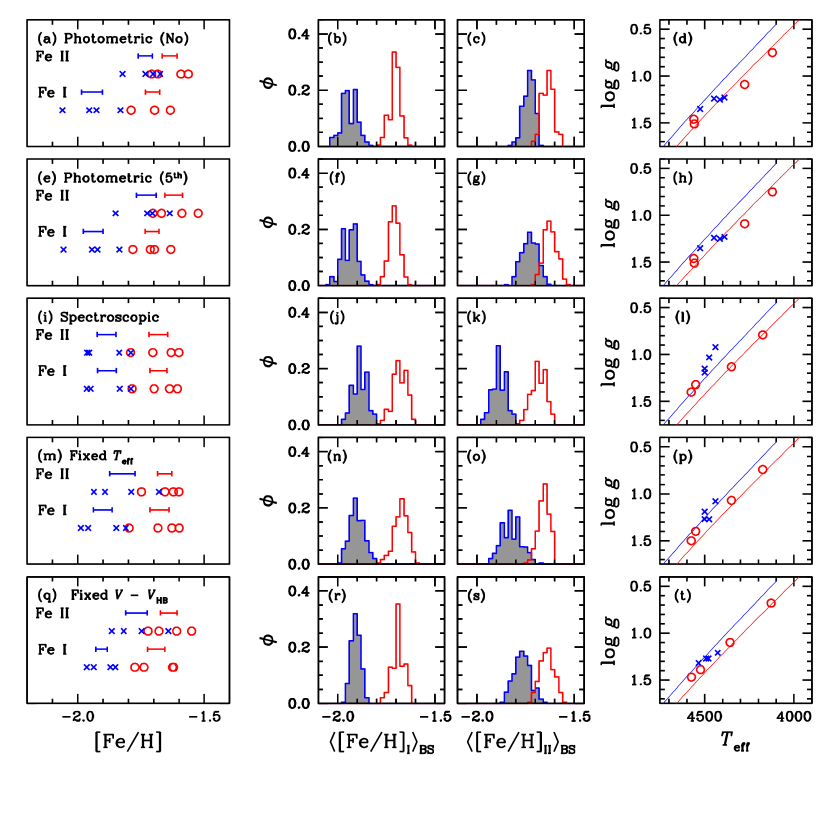
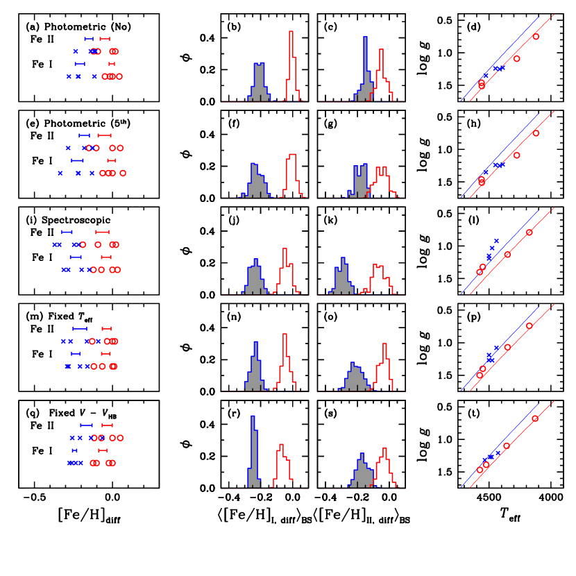
6.1 Photometric method using a single relation
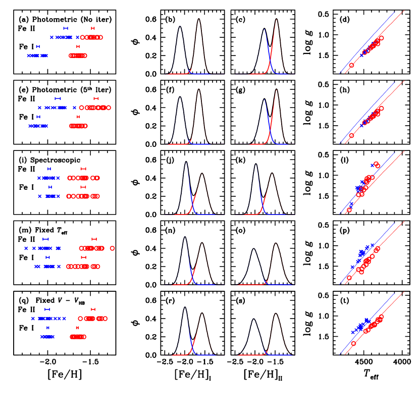
We derive the metallicity of M22 RGB stars based on the photometric effective temperature and surface gravity from our Strömgren photometry of the cluster using the relations by Alonso et al. (1999). During our calculations, we adopted the apparent visual distance modulus of 13.60 mag, = 0.34 and [Fe/H] = 1.65 for M22 (Harris, 1996). As it was done before, we made use of the weak lines only, ) , for both Fe I and Fe II in order to minimize the effect of the adopted micro-turbulent velocity on the metallicity. In Table 2 and Figures 17 and 18, we show our results. For non-differential analysis, the differences in the mean metallicity are [Fe/H]I = 0.239 0.057 dex and [Fe/H]II = 0.096 0.048 dex without iteration, and [Fe/H]I = 0.233 0.048 dex and [Fe/H]II = 0.108 0.052 dex after fifth iteration. Note that our results are consistent with those from the Method 2 by Mu15. In panels (b) and (c) of Figures 17 and 18, we show empirical distributions of the mean [Fe/H]I and [Fe/H]II for the two populations from the bootstrap method, strongly suggest that the metallicity distributions of the two groups of stars in M22 are different. As shown in Table 2, the significance levels to reject the hypothesis that the mean [Fe/H]I values of the - and the - groups are identical are lower than 1%. However, those for [Fe/H]II are rather large, 12 %, for the non-differential analysis. It should not be confused that this rather large significance levels do not indicate that two groups of stars in M22 belong to the same population, but the LTE analysis of the heterogeneous groups of star with a single – relation may be in error.
We also calculate the line-by-line differential iron abundances since the numbers of iron lines being measured by Mu15 for individual stars are different. We selected the star 51 to be the reference star since its and are close to the average for the sample. Also the stellar parameters for this star both from the photometric and spectroscopic methods by Mu15 agree well as shown in Figure 8. For our differential abundance measurements, we did not adjust the stellar parameters of individual stars with respect to the reference star as have done by Yong et al. (2013), for example, and we intended to calculate the proper metallicity offset differences among the sample stars with given stellar parameters. The differences in the mean metallicity from the differential analysis are [Fe/H]I = 0.203 0.039 dex and [Fe/H]II = 0.101 0.045 dex without iteration, and [Fe/H]I = 0.220 0.043 dex and [Fe/H]II = 0.129 0.051 dex with fifth iterations, consistent with those from non-differential analysis. As shown in Table 2, the separation of the mean [Fe/H]II values between the - and the - groups is larger than 2.0 – 2.5 levels. We calculated the significance levels to reject the hypothesis that the mean [Fe/H] values of the two groups of stars in M22 are identical. We obtained the significance levels lower than 1% for [Fe/H]I and 7.5% for [Fe/H]II, strongly suggesting that they are different.
6.2 Spectroscopic method
Next, we derived the metallicity of individual stars based on the spectroscopic and . The differences in the mean metallicity between the two groups of stars are [Fe/H]I = 0.203 0.050 dex and [Fe/H]II = 0.204 0.052 dex for non-differential analysis and [Fe/H]I = 0.194 0.044 dex and [Fe/H]II = 0.228 0.053 dex for differential analysis, making the separation of the mean [Fe/H]II values between the two groups larger than 3.9 to 4.3 levels. Not surprisingly, our results are consistent with those obtained by Marino et al. (2009, 2011), who relied on the traditional spectroscopic stellar parameters. As shown in Table 2, the significance levels to reject the hypothesis that the mean [Fe/H] values of the two groups of stars in M22 are identical are very low, indicating that they are different.
6.3 Using the evolutionary with the spectroscopic
The metallicity based on the evolutionary stellar parameters also suggest that the metallicity distributions of each group of stars are indeed different. Following the same procedure described in §5.4, we obtained the differences in the mean metallicity of [Fe/H]I = 0.224 0.061 dex and [Fe/H]II = 0.168 0.066 dex for non-differential analysis and [Fe/H]I = 0.191 0.043 dex and [Fe/H]II = 0.172 0.060 dex for differential analysis. The mean [Fe/H]II values of each group are different more than 2.5 to 2.9 levels and the low significance levels of being identical distributions also confirm that they are different.
6.4 Using the evolutionary and at a given
Similar conclusion can be drawn when we use the evolutionary and at a given , where we used = 14.15 mag for M22 (Harris, 1996). Following the same procedure described in §5.5, we obtained the differences in the mean metallicity of [Fe/H]I = 0.216 0.047 dex and [Fe/H]II = 0.128 0.062 dex for non-differential analysis and [Fe/H]I = 0.181 0.034 dex and [Fe/H]II = 0.132 0.056 dex for differential analysis. Similar to the results shown above, the mean [Fe/H]II values of each group are different more than 2.1 to 2.4 levels and the low significance levels of being identical distributions also confirm that they are different.
7 SUMMARY
The precision elemental abundance measurement of individual stars in GGs is not a trivial task, especially for a peculiar GC with multiple stellar populations with heterogeneous metallicity distributions. In the context of LTE analysis, our demonstrations with a mock peculiar GC composed of the two normal GCs, NGC 6752 and M55, showed that the internal absolute and the relative metallicity scales are vulnerable to the incorrect treatment of the input stellar parameters among multiple stellar populations with different metallicity. In particular, photometric surface gravity without taking care of proper metallicity effect can result in the [Fe/H]II measurement error of as large as 0.1 – 0.2 dex. As we have discussed earlier, this is because the Fe II line opacity does not vary with surface gravity since the almost all iron atoms are populated in the first ionized level, while the H- continuum opacity is sensitively dependent on the electron pressure and, therefore, surface gravity. As a consequence, changes in surface gravity can mimic the [Fe/H]II abundance of RGB stars in GCs. In this regard, we developed methods independent of the traditional spectroscopic analysis approach, which is demanding excitation and ionization equilibria in Fe I and Fe II elements, to make use of the evolutionary surface gravity. The metallicity scales from these new approaches are in good agreement with those of previous studies by others (Carretta et al., 2009b; Yong et al., 2013).
From our study of a mock peculiar GC, it is worth to mention three comments concerning the metallicity scale of the multiple stellar populations in a GC. First, the use of narrow band photometry, such as and which are sensitive to metallicity and less sensitive to interstellar reddening, is beneficial to discern small [Fe/H] differences. Second, our results show that our adaptive methods to estimate appropriate surface gravity would be essential in deriving the absolute and the relative [Fe/H]II scale for the multiple stellar populations in peculiar GCs. Third, it is very interesting to note that our new methods appear to provide similar metallicity scale as that from the traditional spectroscopic analysis, suggesting that, the metallicity scale from the widely used traditional spectroscopic approach which makes use of excitation and ionization equilibria in Fe I and Fe II elements, is valid, at least in the relative sense.
Contrary to the conclusion made by Mu15, our re-examination of M22 RGB stars showed that the peculiar GC M22 is composed of two groups of stars with heterogeneous metallicities, confirming our previous results and those of others (Lee et al., 2009a; Lee, 2015; Da Costa et al., 2009; Marino et al., 2009, 2011), and the M22 saga will continue.
References
- Alonso et al. (1999) Alonso, A., Arribas, S., & Martínez-Roger, C. 1999, A&AS, 140, 261
- Anthony-Twarog et al. (1995) Anthony-Twarog, B. J., Twarog, B. A., Craig, J. 1995, PASP, 107, 32
- Baines et al. (2010) Baines, E. K. et al. 2010, ApJ, 710, 1365
- Belokurov et al. (2006) Belokurov, V., Zucker, D. B., Evans, N. W., et al. 2006, ApJ, 642, 137
- Bland-Hawthorn& Freeman (2014) Bland-Hawthorn, J., & Freeman, K. 2014, Near Field Cosmology: The Origin of the Galaxy and the Local Group, Saas-Fee Advanced Course, Vol. 37, ed. B. Moore (Berlin, Heidelberg: Springer), 1
- Brown & Wallerstein (1992) Brown, J. W., & Wallerstein, G. 1992, AJ, 104, 1818
- Carretta et al. (2009a) Carretta E., Bragaglia, A., Gratton, R.G., Lucatello S., Cantanzaro G. et al. 2009a, A&A, 505, 117
- Carretta et al. (2009b) Carretta, E., Bragaglia, A., Gratton, R., & Lucatello, S. 2009b, A&A, 505, 139
- Da Costa et al. (2009) Da Costa, G. S., Held, E. V., Saviane, I., & Gullieuszik, M. 2009, ApJ, 705, 1481
- D’Antona & Ventura (2007) D’Antona, F., & Ventura, P. 2007, MNRAS, 379, 1431
- Decressin et al. (2007) Decressin, T., Charbonnel, C., & Meynet, G. 2007, A&A, 475, 859
- D’ercole et al. (2008) D’Ercole, A., Vesperini, E., D’Antona, F., McMillan, S. L. W., & Recchi, S. 2008, MNRAS, 391, 825
- Dotter et al. (2008) Dotter, A., Chaboyer, B., Jevremović, D., Kostov, V., Baron, E., Ferguson, J. W. 2008, ApJS, 178, 89
- Freeman (1993) Freeman, K. C. 1993, in ASP Conf. Ser. 48, The Globular Clusters-Galaxy Connection, eds. G. H. Smith & J. P. Brodie (San Francisco, CA: ASP), 608
- Gray (2008) Gray, D. F. The Observation and Analysis of Stellar Photospheres (3rd ed: Cambridge: Cambridge Univ. Press)
- Harris (1996) Harris, W. E. 1996, AJ, 112, 1487
- Johnson & Pilachowski (2010) Johnson, C. I., & Pilachowski, C. A. 2010, ApJ, 722, 1373
- Joo & Lee (2013) Joo, S.-J., & Lee, Y.-W. 2013, ApJ, 762, 36
- Kraft (1994) Kraft, R. P. 1994, PASP, 106, 553
- Kraft & Ivans (2003) Kraft, R. P., & Ivans, I. I. 2003, PASP, 115, 143
- Lee (2010) Lee, J.-W. 2010, MNRAS, 405, L36
- Lee (2015) Lee, J.-W. 2015, ApJS, 219, 7
- Lee et al. (2004) Lee, J.-W., Carney, B. W., & Balachandran, S. C. 2004, AJ, 128, 2388
- Lee et al. (2005) Lee, J.-W., Carney, B. W., & Habgood, M. J. 2005, AJ, 129, 251
- Lee et al. (2009a) Lee, J.-W., Kang, Y.-W., Lee, J., & Lee, Y.-W. 2009a, Nature, 462, 480
- Lee et al. (2009b) Lee, J.-W., Lee, J., Kang, Y.-W., Lee, Y.-W., Han, S.-I., Joo, S.-J., Rey, S.-C., & Yong, D. 2009b, ApJ, 695, L78
- Lee et al. (2006) Lee, J.-W., López-Morales, M., & Carney, B. W. 2006, ApJ, 646, L119
- Lee et al. (2014) Lee, J.-W., López-Morales, M., Hong, K., Kang, Y.-W., Pohl, B. L., & Walker, A. 2014, ApJS, 210, 6
- Lee et al. (1999) Lee, Y.-W., Joo, J.-M., Sohn, Y.-J., Rey, S.-C., Lee, H.-c., & Walker, A. R. 1999, Nature, 402, 55
- Lim et al. (2015) Lim, D., Han, S.-I., Lee, Y.-W., Roh, D.-G., Sohn, Y.-J., Chun, S.-H., Lee, J.-W., & Johnson, C. I. 2015, ApJS, 216, 19
- Marino et al. (2013) Marino, A. F., Milone, A. P., & Lind, K. 2013, ApJ, 768, 27
- Marino et al. (2009) Marino, A. F., Milone, A. P., Piotto, G., Villanova, S., Bedin, L. R., Bellini, A., & Renzini, A. 2009, A&A, 505, 1099
- Marino et al. (2012) Marino, A. F., Milone, A. P., Sneden, C., Bergemann, M., Kraft, R. P., Wallerstein, G., Cassisi, S., Aparicio, A., Asplund, M., Bedin, R. L., Hilker, M., Lind, K., Momany, Y., Piotto, G., Roederer, I. U., Stetson, P. B., & Zoccali, M. 2012, A&A, 541, 15
- Marino et al. (2011) Marino, A. F., Sneden, C., Kraft, R. P., Wallerstein, G., Norris, J. E., Da Costa, G., Milone, A. P., Ivans, I. I., Gonzalez, G., Fulbright, J. P., Hilker, M., Piotto, G., Zoccali, M., & Stetson, P. B. 2011, A&A, 532, A8
- Moore et al. (1999) Moore, B., Ghigna, S., Governato, F., Lake, G., Quinn, T., Stadel, J., & Tozzi, P. 1999, ApJ, 524, L19
- Mucciarelli et al. (2015) Mucciarelli, A., Lapenna, E., Massari, D., Pancino, E., Stetson, P. B., Ferraro, F. R., Lanzoni, B., & Lardo, C. 2015, ApJ, 809, 128
- Norris & Freeman (1983) Norris, J., & Freeman, K. C. 1983, ApJ, 266, 130
- Searle & Zinn (1978) Searle, L., & Zinn, R. 1978, ApJ, 225, 357
- Sneden (1973) Sneden, C. 1973, PhD thesis, The University of Texas at Austin
- Sneden et al. (1991) Sneden, C., Kraft, R. P., Prosser, C. F., & Langer, G. E. 1991, AJ, 102, 2001
- Thévenin & Idiart (1999) Thévenin, F., & Idiart, T. P. 1999, ApJ, 521, 753
- VandenBerg et al. (2006) VandenBerg, D. A., Bergbusch, P. A., & Dowler, P. D. 2006 ApJS, 162, 375
- Yong et al. (2013) Yong, D., Meléndez, J., Grundahl, F., Roederer, I. U., Norris, J. E., Milone, A. P., Marino, A. F., Coelho, P., McArthur, B. E., Lind, K., Collet, R., & Asplund, M. 2013, MNRAS, 434, 3542
| +50 K | 50 K | +0.2 | 0.2 | ||
|---|---|---|---|---|---|
| [Fe/H]I | 0.044 0.003 | 0.044 0.003 | 0.007 0.002 | 0.000 0.001 | |
| [Fe/H]II | 0.037 0.006 | 0.036 0.005 | 0.090 0.004 | 0.084 0.004 | |
| Method | [Fe/H]I | [Fe/H]II | |||||||
|---|---|---|---|---|---|---|---|---|---|
| t11Student’s -score. | S.L.22The significance level to reject the hypothesis that the mean [Fe/H] values of the - and - groups are identical. | S.L.33The significance level to reject the hypothesis that the mean [Fe/H] values of the - and - groups are identical from bootstrap realization. | t11Student’s -score. | S.L.22The significance level to reject the hypothesis that the mean [Fe/H] values of the - and - groups are identical. | S.L.33The significance level to reject the hypothesis that the mean [Fe/H] values of the - and - groups are identical from bootstrap realization. | ||||
| (%) | (%) | (%) | (%) | ||||||
| Mu15 M2 | 0.232 0.066 | 3.52 | 1.93 | 0.00 | 0.053 0.022 | 2.43 | 8.98 | 0.00 | |
| Mu15 M2 (5th Iter.) | 0.217 0.076 | 2.84 | 3.02 | 3.14 | 0.090 0.041 | 2.20 | 7.24 | 5.57 | |
| + (A99, No Iter.) | 0.239 0.057 | 4.20 | 0.76 | 0.00 | 0.096 0.048 | 2.01 | 9.11 | 11.27 | |
| + (A99, 5th Iter.) | 0.233 0.048 | 4.24 | 0.72 | 0.00 | 0.108 0.052 | 1.80 | 12.32 | 11.42 | |
| Spectroscopic | 0.203 0.050 | 3.48 | 1.32 | 0.00 | 0.204 0.052 | 3.38 | 1.49 | 3.02 | |
| Fixed | 0.224 0.061 | 3.67 | 1.04 | 0.00 | 0.168 0.066 | 2.54 | 5.44 | 2.85 | |
| Fixed | 0.216 0.047 | 4.57 | 0.52 | 0.00 | 0.128 0.062 | 2.08 | 8.56 | 8.46 | |
| Differential Analysis | |||||||||
| Mu15 M2 | 0.213 0.064 | 3.30 | 1.92 | 0.00 | 0.077 0.033 | 2.35 | 8.01 | 2.89 | |
| Mu15 M2 (5th Iter.) | 0.205 0.069 | 2.96 | 2.60 | 2.71 | 0.112 0.036 | 3.08 | 3.10 | 0.00 | |
| + (A99, No Iter.) | 0.203 0.039 | 5.23 | 0.40 | 0.00 | 0.101 0.045 | 2.25 | 6.66 | 5.55 | |
| + (A99, 5th Iter.) | 0.220 0.043 | 4.19 | 0.90 | 0.00 | 0.129 0.051 | 2.19 | 7.33 | 5.74 | |
| Spectroscopic | 0.194 0.044 | 3.79 | 0.92 | 0.00 | 0.228 0.053 | 3.74 | 1.09 | 0.00 | |
| Fixed | 0.191 0.043 | 4.43 | 0.45 | 0.00 | 0.172 0.060 | 2.86 | 3.42 | 2.86 | |
| Fixed | 0.181 0.034 | 5.36 | 0.41 | 0.00 | 0.132 0.056 | 2.36 | 5.67 | 5.61 | |
| Method | gf11 C09 = Carretta et al. (2009b); Y13 = Yong et al. (2013). | M55 | NGC 6752 | 22 = [Fe/H]N6752 [Fe/H]M55 | |||||
|---|---|---|---|---|---|---|---|---|---|
| [Fe/H]I | [Fe/H]II | [Fe/H]I | [Fe/H]II | [Fe/H]I | [Fe/H]II | ||||
| Phot.33Photometric method using two separate relations. | C09 (No) | 2.087 0.018 | 1.936 0.020 | 1.645 0.014 | 1.471 0.015 | 0.443 0.023 | 0.465 0.025 | ||
| C09 (5th) | 2.090 0.016 | 1.927 0.028 | 1.642 0.014 | 1.432 0.024 | 0.448 0.021 | 0.496 0.037 | |||
| Y13 (No) | 2.067 0.016 | 1.896 0.021 | 1.687 0.005 | 1.463 0.006 | 0.379 0.017 | 0.443 0.022 | |||
| Y13 (5th) | 2.073 0.014 | 1.869 0.029 | 1.683 0.005 | 1.414 0.010 | 0.390 0.015 | 0.454 0.031 | |||
| Phot.44Photometric method using a single relation. | C09 (No) | 2.114 0.017 | 1.789 0.022 | 1.645 0.014 | 1.471 0.015 | 0.469 0.022 | 0.318 0.027 | ||
| C09 (5th) | 2.110 0.016 | 1.883 0.030 | 1.642 0.014 | 1.432 0.024 | 0.469 0.021 | 0.451 0.038 | |||
| Y13 (No) | 2.093 0.016 | 1.748 0.022 | 1.687 0.005 | 1.463 0.006 | 0.406 0.017 | 0.285 0.023 | |||
| Y13 (5th) | 2.092 0.015 | 1.825 0.031 | 1.683 0.005 | 1.414 0.010 | 0.409 0.016 | 0.411 0.032 | |||
| Spec. | C09 | 2.003 0.020 | 2.002 0.019 | 1.583 0.027 | 1.584 0.025 | 0.420 0.033 | 0.418 0.031 | ||
| Y13 | 1.952 0.014 | 1.956 0.017 | 1.657 0.003 | 1.635 0.004 | 0.295 0.014 | 0.321 0.017 | |||
| Fixed | C09 | 2.001 0.019 | 2.026 0.030 | 1.579 0.025 | 1.455 0.025 | 0.422 0.031 | 0.571 0.039 | ||
| Y13 | 1.966 0.015 | 1.890 0.028 | 1.655 0.003 | 1.463 0.010 | 0.311 0.015 | 0.426 0.030 | |||
| Fixed | C09 | 1.999 0.009 | 2.006 0.027 | 1.651 0.011 | 1.467 0.021 | 0.348 0.014 | 0.539 0.034 | ||
| Y13 | 2.005 0.008 | 1.943 0.029 | 1.690 0.004 | 1.465 0.010 | 0.315 0.009 | 0.479 0.031 | |||