Hurwitz Number Fields

Abstract.

The canonical covering maps from Hurwitz varieties to configuration varieties are important in algebraic geometry. The scheme-theoretic fiber above a rational point is commonly connected, in which case it is the spectrum of a Hurwitz number field. We study many examples of such maps and their fibers, finding number fields whose existence contradicts standard mass heuristics.

1. Introduction

This paper is a sequel to Hurwitz monodromy and full number fields [19], joint with Venkatesh. It is self-contained and aimed more specifically at algebraic number theorists. Our central goal is to provide experimental evidence for a conjecture raised in [19]. More generally, our objective is to get a concrete and practical feel for a broad class of remarkable number fields arising in algebraic geometry, the Hurwitz number fields of our title.

1.1. Full fields, the mass heuristic, and a conjecture

Say that a degree $m$ number field $K={\mathbb{Q}}[x]/f(x)$ is full if the Galois group of $f(x)$ is either the alternating group $A_{m}$ or the symmetric group $S_{m}$. For $\mathcal{P}$ a finite set of primes, let $F_{\mathcal{P}}(m)$ be the number of full fields $K$ of degree $m$ with all primes dividing the discriminant $\mbox{disc}(K)$ within $\mathcal{P}$.

In [3], Bhargava formulated a heuristic expectation $\mu_{D}(m)$ for the number $F_{D}(m)$ of degree $m$ full number fields with absolute discriminant $D\in{\mathbb{Z}}_{\geq 1}$. The main theorems of [7], [2], and [4] respectively say that this heuristic is asymptotically correct for $m=3$, $4$, and $5$. While Bhargava is clearly focused in [3] on this “horizontal” direction of fixed $m$ and increasing $D$, it certainly makes sense to apply the same mass heuristic in the “vertical” direction. In [16], we summed over contributing $D$ to obtain a heuristic expectation $\mu_{\mathcal{P}}(m)$ for the number $F_{\mathcal{P}}(m)$. Figure 1.1 graphs the function $\mu_{\mathcal{P}}$ in the completely typical case of $\mathcal{P}=\{2,3,5\}$. For any fixed $\mathcal{P}$, the numbers $\mu_{\mathcal{P}}(m)$ can be initially quite large, but by [16, Eq. 68] they ultimately decay super-exponentially to zero. From this mass heuristic, one might expect that for any fixed $\mathcal{P}$, the sequence $F_{\mathcal{P}}(m)$ would be eventually zero.

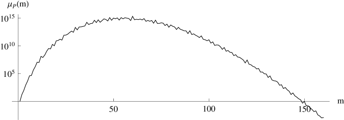
Figure 1.1. The heuristic approximation $\mu_{\mathcal{P}}(m)$ to the number $F_{\mathcal{P}}(m)$ of degree $m$ full fields ramified within $\mathcal{P}=\{2,3,5\}$

The construction studied in [19] has origin in work of Hurwitz and involves an arbitrary finite nonabelian simple group $T$. Let $\mathcal{P}_{T}$ be the set of primes dividing $T$. The construction gives a large class of separable algebras $K_{h,u}$ over ${\mathbb{Q}}$ which we call Hurwitz number algebras. Infinitely many of these algebras have all their ramification with $\mathcal{P}_{T}$. Within the range of our computations here, these algebras are commonly number fields themselves; in all cases, they factor into number fields which we call Hurwitz number fields. The algebras come in families of arbitrary dimension $\rho\in{\mathbb{Z}}_{\geq 0}$, with the Hurwitz parameter $h$ giving the family and the specialization parameter $u$ giving the member of the family. Strengthening Conjecture 8.1 of [19] according to the discussion in §8.5 there, we expect that there are enough contributing $K_{h,u}$ to give the following statement.

Conjecture 1.1.

Suppose $\mathcal{P}$ contains the set of primes dividing the order of a finite nonabelian simple group. Then the sequence $F_{\mathcal{P}}(m)$ is unbounded.

From the point of view of the mass heuristic, the conjecture has both an unexpected hypothesis and a surprising conclusion.

1.2. Content of this paper

The parameter numbers $\rho=0$ and $1$ have special features connected to dessins d’enfants, and we are presenting families with $\rho\in\{0,1\}$ in [15]. To produce enough fields to prove Conjecture 1.1, it is essential to let $\rho$ tend to infinity. Accordingly we concentrate here on the next case $\rho=2$, with our last example being in the setting $\rho=3$.

Section 2 serves as a quick introduction. Without setting up any general framework, it exhibits a degree $25$ family. Specializing this family gives more than $10,000$ number fields with Galois group $S_{25}$ or $A_{25}$ and discriminant of the form $\pm 2^{a}3^{b}5^{c}$.

Section 3 introduces Hurwitz parameters and describes how one passes from a parameter to a Hurwitz cover. Full details would require deep forays into moduli problems on the one hand and braid group techniques on the other. We present information at a level adequate to provide a framework for our examples to come. In particular, we use the Hurwitz parameter $h=(S_{5},(2111,5),(4,1))$ corresponding to our introductory example to illustrate the generalities.

Section 4 focuses on specialization, meaning the passage from a Hurwitz cover to its fibers. In the alternative language that we have been using in this introduction, a Hurwitz cover gives a family of Hurwitz number algebras, and then specialization is passing from the entire family to one of its members. The section elaborates on the heuristic argument for Conjecture 1.1 given in [19]. It formulates Principles A, B, and C, all of which say that specialization behaves close to generically. Proofs of even weak forms of Principles A and B would suffice to prove Conjecture 1.1. Here again, the introductory example is used to illustrate the generalities.

The slightly shorter Sections 5-10 each report on a family and its specializations, degrees being $9$, $52$, $60$, $96$, $202$, and $1200$. Besides describing its family, each section also illustrates a general phenomenon.

Sections 5-10 together indicate that the strength with which Principles A, B, and C hold has a tendency to increase with the degree $m$, in strong support of Conjecture 1.1. In particular, our two largest degree examples clearly show that Hurwitz number fields are not governed by the mass heuristic as follows. In the degree $202$ family, Principles A, B, and C hold without exception. One has $\mu_{\{2,3,5\}}(202)\approx 2\cdot 10^{-17}$, but the family shows $F_{\{2,3,5\}}(202)\geq 2947$. Similarly, $\mu_{\{2,3,5\}}(1200)\approx 10^{-650}$ while the one specialization point we look at in the degree $1200$ family shows $F_{\{2,3,5\}}(1200)\geq 1$.

There are hundreds of assertions in this paper, with proofs in most cases involving computer calculations, using Mathematica [23], Pari [21], and Magma [5]. We have aimed to provide an accessible exposition which should make all the assertions seem plausible to a casual reader. We have also included enough details so that a diligent reader could efficiently check any of these assertions. Both types of readers could make use of the large Mathematica file HNF.mma on the author’s homepage. This file contains seven large polynomials defining the seven families considered here, and miscellaneous further information about their specialization to number fields.

1.3. Acknowledgements

This paper was started at the same time as [19]. It is a pleasure to thank Akshay Venkatesh whose careful reading of early drafts of this paper in the context of its relation with [19] improved it substantially. It is also a pleasure to thank the Simons foundation which partially supported this work through grant #209472.

2. A degree $25$ introductory family

In this section, we begin by constructing a single full Hurwitz number field, of degree $25$ and discriminant $2^{56}3^{34}5^{30}$. We then use this example to communicate the general nature of Hurwitz number fields and their explicit construction. We close by varying two parameters involved in the construction to get more than ten thousand other degree twenty-five full Hurwitz number fields from the same family, all ramified within $\{2,3,5\}$.

2.1. The $25$ quintics with critical values $-2$, $0$, $1$ and $2$

Consider polynomials in ${\mathbb{C}}[s]$ of the form

(2.1) $$g(s)=s^{5}+bs^{3}+cs^{2}+ds+x.$$

We will determine when the set of critical values of $g(s)$ is $\{-2,0,1,2\}$.

The critical points of such a polynomial are of course given by the roots of its derivative $g^{\prime}(s)$. The critical values are then given by the roots of the resultant

$$r(t)=\mbox{Res}_{s}(g(s)-t,g^{\prime}(s)).$$

Explicitly, this resultant works out to $r(t)=$

$$3125t^{4}$$

$$+1250(3bc-10x)t^{3}$$

$$+\left(108b^{5}-900b^{3}d+825b^{2}c^{2}-11250bcx+2000bd^{2}+2250c^{2}d+18750x^{2}\right)t^{2}$$

$$-2\left(108b^{5}x-36b^{4}cd+8b^{3}c^{3}-900b^{3}dx+825b^{2}c^{2}x+280b^{2}cd^{2}\right.$$

$$\left.\qquad-315bc^{3}d-5625bcx^{2}+2000bd^{2}x+54c^{5}+2250c^{2}dx-800cd^{3}+6250x^{3}\right)t$$

$$+\left(108b^{5}x^{2}-72b^{4}cdx+16b^{4}d^{3}+16b^{3}c^{3}x-4b^{3}c^{2}d^{2}-900b^{3}dx^{2}+825b^{2}c^{2}x^{2}\right.$$

$$\left.\qquad+560b^{2}cd^{2}x-128b^{2}d^{4}-630bc^{3}dx+144bc^{2}d^{3}-3750bcx^{3}\right.$$

$$\left.\qquad+2000bd^{2}x^{2}+108c^{5}x-27c^{4}d^{2}+2250c^{2}dx^{2}-1600cd^{3}x+256d^{5}+3125x^{4}\right).$$

This large expression conforms to the a priori known structure of $r(t)$: it is a quartic polynomial in the variable $t$ depending on the four parameters $b$, $c$, $d$, and $x$. The computation required to obtain the expression is not at all intensive; for example, Mathematica’s Resultant does it in $0.01$ seconds of CPU-time.

Now consider in general the problem of classifying quintic polynomials (2.1) with prescribed critical values. Clearly, if the given values are the roots of a monic degree four polynomial $\tau(t)$, then we need to choose the $b$, $c$, $d$, and $x$ so that $r(t)$ is identically equal to $3125\tau(t)$. Equating coefficients of $t^{i}$ for $i=0$, $1$, $2$, and $3$ gives four equations in the four unknowns $b$, $c$, $d$, and $x$. If $(b,c,d,x)$ is a solution then so is $(\omega^{2}b,\omega^{3}c,\omega^{4}d,\omega^{5}x)$ for any fifth root of unity $\omega$. Thus the solutions come in packets of five, each packet having a common $x$.

In our explicit example, $\tau(t)=(t+2)t(t-1)(t-2)$. Mathematica determines in less than a second that there are 125 solutions $(b,c,d,x)$. The twenty-five possible $x$’s are the roots of a degree twenty-five polynomial,

(2.2) $$f(x)=2^{98}3^{8}x^{25}-2^{96}3^{8}5^{2}x^{24}+\cdots+4543326944239835953052526892234.$$

The algebra ${\mathbb{Q}}[x]/f(x)$ is our first explicit example of a Hurwitz number algebra. In this case, $f(x)$ is irreducible in ${\mathbb{Q}}[x]$, so that ${\mathbb{Q}}[x]/f(x)$ is in fact a Hurwitz number field.

2.2. Real and complex pictures

Before going on to arithmetic concerns, we draw two pictures corresponding to the Hurwitz number field ${\mathbb{Q}}[x]/f(x)$ we have just constructed. Any Hurwitz number algebra $K$ would have analogous pictures. Our object is to visually capture the fact that any Hurwitz number algebra $K$ is involved in a very rich mathematical situation. Indeed if $K$ has degree $m$, then one has $m$ different geometric objects, with their arithmetic coordinated by $K$.

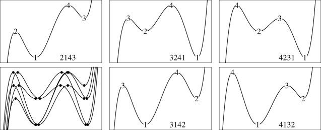
Figure 2.1. Graphs $t=g_{x}(s)$ of five quintic polynomials with critical points $(s_{i},t_{i})$ ordered from bottom to top and marked by $i\in\{1,2,3,4\}$.

Of the twenty-five solutions $x$ to (2.2), five are real. Each of these $x$ corresponds to exactly one real solution $(b,c,d,x)$. The corresponding polynomials $g_{x}(s)$ are plotted in the window $[-2.1,2.1]\times[-2.4,2.4]$ of the real $s$-$t$ plane in Figure 2.1. The critical values $t_{i}$ are indexed from bottom to top so that always $(t_{1},t_{2},t_{3},t_{4})=(-2,0,1,2)$, with $i$ printed at the corresponding turning point $(s_{i},t_{i})$. The labeling of each graph encodes the left-to-right ordering of the critical points $s_{i}$. For example, in the upper left rectangle the critical points are $(s_{2},s_{1},s_{4},s_{3})\approx(-1.5,-0.6,0.7,1.4)$ and the graph is accordingly labeled by $L=2143$. The labeling is consistent with the labeling in Figure 2.4 below.

To get images for all twenty-five roots $x$, we consider the semicircular graph ​\Rightcircle in the complex $t$-plane drawn in Figure 2.3. We then draw in Figure 2.4 its preimage $g_{x}^{-1}(\mbox{\begin{sideways} {\!\lx@text@nounicode\Rightcircle\,} \end{sideways}})$ in the complex $s$-plane under twenty-five representatives $g_{x}$. Each of the four critical values $t_{i}\in\{-2,0,1,2\}$ has a unique critical preimage $s_{i}\in{\mathbb{C}}$, and we print $i$ at $s_{i}$ in Figure 2.4. There are braid operations $\sigma_{1}$, $\sigma_{2}$, $\sigma_{3}$ corresponding to universal rules which permute the figures, given in this instance by Figure 2.3. Here the $\sigma_{i}$ all have cycle type $3^{5}2^{5}$ with $\sigma_{2}$ preserving the letter and incrementing the index modulo $3$. The fact that this geometric action has image all of $S_{25}$ suggests that the Galois group of (2.2) will be $A_{25}$ or $S_{25}$ as well.

 

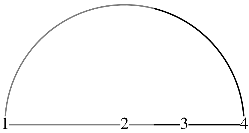
Figure 2.2. A graph connecting the roots of the specialization polynomial $(t+2)t(t-1)(t-2)$

 

Figure 2.3. Actions of $\sigma_{1}$ (vertical arrows), $\sigma_{2}$ (symbols), and $\sigma_{3}$ (horizontal arrows)

The twenty-five preimages are indeed topologically distinct. Thus for the twelve $\gamma_{abc}=\gamma_{cba}$, the critical points $a$, $b$, and $c$ are connected by a triangle and the middle index $b$ is connected also to the remaining critical point. Similarly the indexing for the twelve $\gamma_{abcd}=\gamma_{dcba}$ describes how the critical points are connected. The five graphs corresponding to the real $x$ treated in Figure 2.1 are easily identified by the horizontal line present in Figure 2.4.

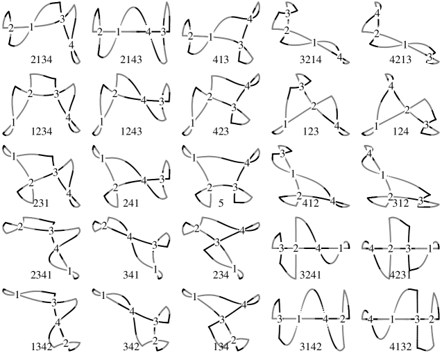
Figure 2.4. The preimage of the semicircular graph of Figure 2.3 under twenty-five quintic polynomials

We are touching on the braid-theoretic infrastructure of Hurwitz number fields in this paper only very lightly. Our point in presenting Figures 2.3-2.4 is simply to give some idea of the topology behind the existence of Hurwitz number fields.

2.3. A better defining polynomial $\phi(x)$ and field invariants.

We are not so much interested in the polynomial $f(x)$ from (2.2) itself, but rather in the field ${\mathbb{Q}}[x]/f(x)$ it defines. Pari’s command polredabs converts $f(x)$ into a monic polynomial $\phi(x)$ which defines the same field and has minimal sum of the absolute squares of its roots. It returns

$$\phi(x)=$$

$$x^{25}-5x^{24}+15x^{23}-5x^{22}-380x^{21}+1290x^{20}-4500x^{19}-28080x^{18}$$

$$+183510x^{17}+74910x^{16}-3033150x^{15}+4181370x^{14}+27399420x^{13}$$

$$-48219480x^{12}-124127340x^{11}+266321580x^{10}+466602765x^{9}$$

$$-592235505x^{8}-905951965x^{7}+1232529455x^{6}+2423285640x^{5}$$

$$+664599470x^{4}-814165000x^{3}-517891860x^{2}-58209720x+2436924.$$

For fields of sufficiently small degree, one applies the reduction operation polredabs as a matter of course: the new smaller-height polynomials are more reflective of the complexity of the fields considered, isomorphic fields may be revealed, and any subsequent analysis of field invariants is sped up.

Pari’s nfdisc calculates that the discriminant of ${\mathbb{Q}}[x]/\phi(x)$ is

$$D=1119186718586212624367616000000000000000000000000000000=2^{56}3^{34}5^{30}.$$

The fact that $D$ factors into the form $2^{a}3^{b}5^{c}$ is known from the general theory presented in Sections 3 and 4, using that $2$, $3$, and $5$ are the primes less than or equal to the degree $5$, and the polynomial discriminant of $\tau(t)=(t+2)t(t-1)(t-2)$, namely $2304=2^{8}3^{2}$, has this form too. Note that since all the exponents of the field discriminant are greater than the degree $25$, the number field is wildly ramified at all the base primes, $2$, $3$, and $5$.

To look more closely at ${\mathbb{Q}}[x]/\phi(x)$, we factorize the $p$-adic completion ${\mathbb{Q}}_{p}[x]/\phi(x)$ as a product of fields over ${\mathbb{Q}}_{p}$. We write the symbol $e^{f}_{c}$ to indicate a factor of degree $ef$, ramification index $e$, and discriminant $p^{fc}$. One gets

$$2 {\bf 16}_{50}\,3_{2}\,3_{2}\,3_{2},$$-adically:

(2.3) $$3 {\bf 9}_{18}\,4_{3}\,4_{3}\,{\bf 3}_{5}\,{\bf 3}_{5}\,1^{2}_{0},$$-adically:

$$5 {\bf 25}_{30},$$-adically:

with wild factors printed in bold. Thus, the first line means that ${\mathbb{Q}}_{2}[x]/\phi(x)$ is a product $K_{1}\times K_{2}\times K_{3}\times K_{4}$, where $K_{1}$ is a wild totally ramified degree sixteen extension of ${\mathbb{Q}}_{2}$ with discriminant $2^{50}$, while $K_{2}$, $K_{3}$, and $K_{4}$ are tame cubic extensions of discriminant $2^{2}$. The behavior for the three primes is roughly typical, although, as we’ll see in Figure 4.2, a little less ramified than average.

Because the field discriminant is a square, the Galois group of $\phi(x)$ is in $A_{25}$. Many small collections of $p$-adic factorization patterns for small unramified $p$ each suffice to prove that the Galois group is indeed all of $A_{25}$. Most easily, $\phi(x)$ factors in ${\mathbb{Q}}_{19}[x]$ into irreducible factors of degrees $17$, $6$, and $2$, so that the Galois group contains an element of order $17$. Jordan’s criterion now applies: a transitive subgroup of $S_{m}$ containing an element of prime order in $(m/2,m-2]$ is all of $A_{m}$ or $S_{m}$. We will use this easy technique without further comment for all of our other determinations that Galois groups of number fields are full. One could also use information from ramified primes as above, but unramified primes give the easiest computational route.

2.4. A family of degree $25$ number fields

We may ask, more generally, for the quintics with any fixed set of critical values. This amounts to repeating our previous computation, replacing the polynomial $\tau(t)=(t+2)t(t-1)(t-2)$ of the three previous subsections with other separable quartic polynomials

(2.4) $$\tau(t)=t^{4}+b_{1}t^{3}+b_{2}t^{2}+b_{3}t+b_{4}.$$

From each such $\tau$, we obtain a degree $25$ algebra over ${\mathbb{Q}}$, once again the algebra determined by the possible values of the variable $x$.

Changing $\tau$ via a rational affine transformation $t\rightarrow\alpha t+\beta$ does not change the degree twenty-five algebra constructed. Accordingly, one can restrict attention to specialization polynomials $\tau(t)$ with $b_{1}=0$, and consider only a set of representatives for the equivalence $(b_{2},b_{3},b_{4})\sim(\alpha^{2}b_{2},\alpha^{3}b_{3},\alpha^{4}b_{4})$, where $\alpha$ is allowed to be in ${\mathbb{Q}}^{\times}$. In particular, if $b_{2}$ and $b_{3}$ are nonzero, any such polynomial is equivalent to a unique polynomial of the form

(2.5) $$\tau(u,v,t)=t^{4}-2t^{2}v-8tv^{2}-4uv^{2}+v^{2}.$$

Here the reason for the complicated form on the right is explained in the discussion around (3.4). We will treat in what follows only the main two-parameter family where $b_{2}$ and $b_{3}$ are both nonzero. Note, however, that two secondary one-parameter families are also interesting: if $b_{3}=0$, one gets degree $25$ algebras with Galois group in $S_{5}\times S_{2}\wr S_{10}$, because of the symmetry induced from $t\mapsto-t$; the case $b_{2}=0$ gives rise to full degree $25$ algebras, just like the main case.

One can repeat the computation of §2.1, now with the parameters $u$ and $v$ left free. The corresponding general degree twenty-five moduli polynomial $f_{25}(u,v,x)$ has $129$ terms as an expanded polynomial in ${\mathbb{Z}}[u,v,x]$. After replacing $x$ by $5x/4$ and clearing a constant, coefficients average about $16$ digits. We will not write this large polynomial explicitly here, instead giving a simpler polynomial that applies only in the special case $u=1/3$ at the end of §4.2.

2.5. Keeping ramification within $\{2,3,5\}$

Suppose $\tau(t)$ from (2.4) normalizes to $\tau(u,v,t)$ from (2.5). We write the corresponding Hurwitz number algebra as $K_{u,v}$. Inclusion (3.14) below says that if $\tau(t)$ is ramified within $\mathcal{P}=\{2,3,5\}$, then so is $K_{u,v}$. By a computer search we have found $11031$ such $(u,v)$. From irreducible $f_{25}(u,v,x)$, we obtain $F_{\mathcal{P}}(25)\geq 10938$. The remaining $f_{25}(u,v,x)$ all have a single rational root and from these polynomials we obtain $F_{\mathcal{P}}(24)\geq 93$. The behavior of the $11031$ different $K_{u,v}$ will be discussed in more detail in Section 4 below.

A point to note is that ramification is obscured by the passage to standardized coordinates. In the case of our first example $\tau(t)=(t+2)t(t-1)(t-2)$, the corresponding $(u,v)$ is $(37/175,9/1715)$. The standardized polynomial $\tau(37/175,9/1715,t)$ after clearing denominators has a $7$ in its discriminant.

3. Background on Hurwitz covers

In this section, we provide general background on Hurwitz covers. Most of our presentation is in the setting of algebraic geometry over the complex numbers. In the last subsection, we shift to the more arithmetic setting where Hurwitz number fields arise.

3.1. Hurwitz parameters

We use the definition in [19, §1B] of Hurwitz parameter: Let $r\in{\mathbb{Z}}_{\geq 3}$. An $r$-point Hurwitz parameter is a triple $h=(G,C,\nu)$ where

$\bullet\;$ $G$ is a finite group;

$\bullet\;$ $C=(C_{1},\dots,C_{k})$ is a list of conjugacy classes whose union generates $G$;

$\bullet\;$ $\nu=(\nu_{1},\dots,\nu_{k})$ is a list of positive integers summing to $r$ such that $\prod[C_{i}]^{\nu_{i}}=1$ in the abelianization $G^{\rm ab}$. We henceforth always take the $C_{i}$ distinct and not the identity, and normalize so that $\nu_{i}\geq\nu_{i+1}$. The number $\nu_{i}$ functions as a multiplicity for the class $C_{i}$.

Table 3.1 gives the Hurwitz parameters of the seven Hurwitz covers described in this paper. It is also gives the associated degrees $m$ and bad reduction sets $\mathcal{P}_{h}$, each to be discussed later in this section.

$$\begin{array}[]{r| lll | rl}\mbox{Section}&G&C&\nu&m&\mathcal{P}_{h}\\ \hline\cr\mbox{\S\ref{deg25a}}&S_{5}&(2111,5)&(4,1)&25&\{2,3,5\}\\ \mbox{\S\ref{deg9}}&S_{3}\wr S_{2}&(21111,33,222)&(3,1,1)&9&\{2,3\}\\ \mbox{\S\ref{deg52}}&S_{6}&(21111,222,3_{1}111,3_{\infty}2_{0}1)&(2,1,1,1)&52&\{2,3,5\}\\ \mbox{\S\ref{deg60}}&PSL_{3}(3)&(2^{4}1^{5},3^{3}1^{4})&(3,2)&2\cdot 60&\{2,3\}\\ \mbox{\S\ref{deg96}}&GL_{3}(2)&(22111,421)&(4,1)&2\cdot 96&\{2,3,7\}\\ \mbox{\S\ref{deg202}}&S_{6}&(21111,3_{0}21,3_{1}111,4_{\infty}11)&(2,1,1,1)&202&\{2,3,5\}\\ \mbox{\S\ref{deg1200}}&S_{6}&(21111,321,411)&(4,1,1)&1200&\{2,3,5\}\end{array}$$

Table 3.1. Hurwitz parameters for the seven covers pursued in this paper, two of them with normalizations given via subscripts

In the case that $G$ is a symmetric group $S_{n}$, we label a conjugacy class $C_{i}$ by the partition $\lambda_{i}$ of $n$ giving the lengths of the cycles of any of its elements. We describe classes for general $G$ in a similar way. Namely we choose a transitive embedding $G\subseteq S_{n}$. We then label classes $C_{i}$ by their induced cycle partitions $\lambda_{i}$, removing any ambiguities which arise by further labeling. In none of our examples is further labeling necessary.

Our concept of Hurwitz parameter emphasizes multiplicities more than other similar concepts in the literature. For example, the first line of Table 3.1 says that our introductory example comes from the parameter $h=(S_{5},(2111,5),(4,1))$. In e.g. [13], the indexing scheme would center on the class vector $(2111,2111,2111,2111,5)$.

3.2. Covers indexed by a parameter

An $r$-point parameter $h=(G,C,\nu)$ determines an unramified cover of $r$-dimensional complex algebraic varieties

(3.1) $$\pi_{h}:{\sf Hur}_{h}\rightarrow{\sf Conf}_{\nu}.$$

The base is the variety whose points are tuples $(D_{1},\dots,D_{k})$ of disjoint subsets $D_{i}$ of the complex projective line ${\sf P}^{1}$, with $D_{i}$ consisting of $\nu_{i}$ points. Above a point $u=(D_{1},\dots,D_{k})\in{\sf Conf}_{\nu}$, the fiber has one point for each solution of a moduli problem indexed by $(h,u)$.

The moduli problem described in [19, §2] involves degree $|G|$ Galois covers $\Sigma\rightarrow{\sf P}^{1}_{t}$, with Galois group identified with $G$. An equivalent version of this moduli problem makes reference to the embedding $G\subseteq S_{n}$ used to label conjugacy classes. When $G$ is its own normalizer in $S_{n}$, which is the case for all our examples, the equivalent version is easy to formulate: above a point $u=(D_{1},\dots,D_{k})\in{\sf Conf}_{\nu}$, the fiber $\pi_{h}^{-1}(u)$ consists of points $x$ indexing isomorphism classes of degree $n$ covers

(3.2) $${\sf S}_{x}\rightarrow{\sf P}_{t}^{1}.$$

These covers are required to have global monodromy group $G$, local monodromy class $C_{i}$ for all $t\in D_{i}$, and be otherwise unramified. In this equivalent version, the ramification numbers of the preimages of $t\in D_{i}$ in ${\sf S}_{x}$ together form the partition $\lambda_{i}$.

We prefer the equivalent version for the purposes of this paper, since it directly guides our actual computations. For example, in our introductory example, the quintic polynomials prominent there can be understood as degree five rational maps ${\sf P}^{1}_{s}\rightarrow{\sf P}^{1}_{t}$. Here ${\sf P}^{1}_{s}$ is a common coordinatized version of all the ${\sf S}_{x}$. Also the preimage of $\infty$ consists of the single point $\infty$, explaining why polynomials rather than more general rational functions are involved. At no point did degree $120$ maps explicitly enter into the computations of Section 2.

3.3. Covering genus

Let $h=(G,C,\nu)$ be a Hurwitz parameter with $G\subseteq S_{n}$ a transitive permutation group. Let $\ell_{i}$ be the the number of parts of the partition $\lambda_{i}$ induced by $C_{i}$, and let $d_{i}=n-\ell_{i}$ be the corresponding drop. Consider the Hurwitz covers ${\sf S}_{x}\rightarrow{\sf P}^{1}_{t}$ parametrized by $x\in{\sf Hur}_{h}$. By the Riemann-Hurwitz formula, the curves ${\sf S}_{x}$ all have genus $g=1-n+\frac{1}{2}\sum\nu_{i}d_{i}$.

Given $G$, let $d$ be the minimal drop of a nonidentity element. If $h$ is an $r$-point Hurwitz parameter based on $G$, then necessarily $g\geq 1-n+dr/2$. To support Conjecture 1.1, one needs to draw fields from cases with arbitrarily large $r$ and thus arbitrarily large $g$. However explicit computation of families rapidly becomes harder as $g$ increases, and in this paper we only pursue cases with genus zero.

3.4. Normalization

The three-dimensional complex group ${\sf PGL}_{2}$ acts by fractional linear transformations on ${\sf Conf}_{\nu}$. Since ${\sf PGL}_{2}$ is connected, the action lifts uniquely to an action on ${\sf Hur}_{h}$ making $\pi_{h}$ equivariant. To avoid redundancy, it is important for us to use this action to replace (3.1) by a cover of varieties of dimension $\rho=r-3$. Rather than working with quotients in an abstract sense, we work with explicit codimension-three slices as follows.

We say that a Hurwitz parameter is base normalizable if $k\geq 3$ and $\nu_{k-2}=\nu_{k-1}=\nu_{k}=1$. For a base normalizable Hurwitz parameter, we replace (3.1) by a map of $\rho$-dimensional varieties,

(3.3) $$\pi_{h}:{\sf X}_{h}\rightarrow{\sf U}_{\nu}.$$

Here the target ${\sf U}_{\nu}$ is the subvariety of ${\sf Conf}_{\nu}$ with $(D_{k-2},D_{k-1},D_{k})=(\{0\},\{1\},\{\infty\})$. The domain ${\sf X}_{h}$ is just the preimage of ${\sf U}_{\nu}$ in ${\sf Hur}_{h}$. This reduction in dimension is ideal for our purposes: each ${\sf PGL}_{2}$ orbit on ${\sf Conf}_{\nu}$ contains exactly one point in ${\sf U}_{\nu}$.

We say that a base normalizable genus zero Hurwitz parameter is fully normalizable if the partitions $\lambda_{k-2}$, $\lambda_{k-1}$, and $\lambda_{k}$ have between them at least three singletons. A normalization is then obtained by labeling three of the singletons by $0$, $1$, and $\infty$, as illustrated twice in Table 3.1. This labeling places a unique coordinate function $s$ on each ${\sf S}_{x}$. Accordingly, each point of ${\sf X}_{h}$ is then identified with an explicit rational map from ${\sf P}_{s}^{1}\rightarrow{\sf P}_{t}^{1}$.

When the above normalization conventions do not apply, we modify the procedure, typically in a very slight way, so as to likewise replace the cover of $r$-dimensional varieties (3.1) by a cover of $\rho$-dimensional varieties (3.3). For example, two other multiplicity vectors $\nu$ figuring into some of our examples are $(4,1)$ and $(3,1,1)$. For these cases, we define

$$\tau_{4}(t) =t^{4}-2t^{2}v-8tv^{2}-4uv^{2}+v^{2}, \tau_{3}(t) =t^{3}+t^{2}+ut+v.$$

The form for $\tau_{4}(t)$ is chosen to make discriminants tightly related:

(3.4) $$\mbox{disc}_{t}(\tau_{4}(t)) =-2^{12}v^{6}d, \mbox{disc}_{t}(t\tau_{3}(t)) =vd,$$

with

(3.5) $$d=4u^{3}-u^{2}-18uv+27v^{2}+4v.$$

In the respective cases, we say that a divisor tuple is normalized if it has the form

$$(D_{1},D_{2}) =((\tau_{4}(t)),\{\infty\}), (D_{1},D_{2},D_{3}) =((\tau_{3}(t)),\{0\},\{\infty\}).$$

These normalization conventions define subvarieties ${\sf U}_{4,1}\subset{\sf Conf}_{4,1}$ and ${\sf U}_{3,1,1}={\sf Conf}_{3,1,1}$. As explained in the $(4,1)$ setting in §2.4, we are throwing away some perfectly interesting ${\sf PGL}_{2}$ orbits on ${\sf Conf}_{\nu}$ by our somewhat arbitrary normalization conventions. However all these orbits together have positive codimension in ${\sf Conf}_{\nu}$ and what is left is adequate for our purposes of supporting Conjecture 1.1. Always, once we have ${\sf U}_{\nu}\subset{\sf Conf}_{\nu}$ we just take ${\sf X}_{h}\subset{\sf Hur}_{h}$ to be its preimage.

The two base varieties just described are identified by their common coordinates: ${\sf U}_{4,1}={\sf U}_{3,1,1}=\mathrm{Spec}\,{\mathbb{C}}[u,v,1/vd]$. This exceptional identification has a conceptual source as follows. With $(u,v)$ fixed, let $D_{1}=(\tau_{4}(u,v,t))$ so that $(D_{1},\{\infty\})\in{\sf U}_{4,1}$. Let $V$ be the four-element subgroup of ${\sf PGL}_{2}$ consisting of fractional transformations stabilizing the roots of $\tau_{4}(u,v,t)$. One then has a degree four map $q$ from ${\sf P}^{1}_{t}$ to its quotient ${\sf P}:={\sf P}^{1}_{t}/V$. There are three natural divisors on ${\sf P}$: the divisor $\Delta_{1}$ consisting of the three critical values, and the one-point divisors $\Delta_{2}=\{q(D_{1})\}$ and $\Delta_{3}=\{q(\infty)\}$. Uniquely coordinatize ${\sf P}$ so that $(\Delta_{1},\Delta_{2},\Delta_{3})=((\tau_{3}(u^{\prime},v^{\prime},t)),\{0\},\{\infty\})$. Then $u^{\prime}=u$ and $v^{\prime}=v$.

3.5. The mass formula and braid representations

The degree $m$ of a cover ${\sf X}_{h}\rightarrow{\sf U}_{\nu}$ can be calculated by group-theoretic techniques as follows. Define the mass $\overline{m}$ of an $r$-point Hurwitz parameter $h=(G,C,\nu)$ via a sum over the irreducible characters of $G$:

(3.6) $$\overline{m}=\frac{\prod_{i}|C_{i}|^{\nu_{i}}}{|G|^{2}}\sum_{\chi\in\widehat{G}}\frac{\prod_{i}\chi(C_{i})^{\nu_{i}}}{\chi(1)^{r-2}}.$$

Then $\overline{m}\geq m$ always. Suppose that no proper subgroup $H\subset G$ contains elements from all the conjugacy classes $C_{i}$, as is the case in §§2, 5, 6. Then $\overline{m}=m$. When there are exist such $H$, as in §§7, 8, 9, and 10, one can still get exact degrees by applying (3.6) to all such $H$ and computing via inclusion-exclusion. Chapter 7 of [20] gives (3.6) and works out several examples in the setting $r=3$.

As a one-parameter collection of examples, consider $h(j)=(S_{5},(2111,5),(j,1))$ for $j\geq 4$ even. Since $S_{5}$ is generated by any $5$-cycle and any transposition, one has $\overline{m}=m$ for $h(j)$. From $0$’s in the character table of $S_{5}$, only the characters $1$, $\epsilon$, $\chi$, and $\chi\epsilon$ contribute, with $\epsilon$ the sign character and $\chi+1$ the given degree $5$ permutation character. We can ignore $\epsilon$ and $\chi\epsilon$ by doubling the contribution of $1$ and $\chi$:

$$m=\frac{10^{j}24}{120^{2}}\left(2+2\frac{\chi(2111)^{j}\chi(5)}{\chi(1)^{r-1}}\right)=\frac{10^{j-2}}{6}\left(2+2\cdot\frac{2^{j}(-1)}{4^{j-1}}\right)=\frac{1}{3}\left(10^{j-2}-5^{j-2}\right).$$

For $j=4$, one indeed has $m=25$, as in the introductory example.

The monodromy group of a cover ${\sf X}_{h}\rightarrow{\sf U}_{\nu}$ can be calculated by group-theoretic techniques [19, §3]. These techniques center on braid groups and underlie the mass formula. The output of these calculations is a collection of permutations in $S_{m}$ which generate the monodromy group, with $\langle\sigma_{1},\sigma_{2},\sigma_{3}\rangle=S_{25}$ from Figure 2.3 being completely typical. Fullness of these representations is important for us: once we switch over to the arithmetic setting in §3.8, it implies fullness of generic specializations.

Theorem 5.1 of [19] proves a general if-and-only-if result about fullness. In one direction, the important fact for us here is that to systematically obtain fullness one needs for $G$ to be very close to a nonabelian simple group $T$. Here “very close” includes subgroups of $\mbox{Aut}(T)$ of the form $T.2$, such as $G=S_{n}$ for $T=A_{n}$. This direction accounts for the hypothesis of Conjecture 1.1. In the other direction, fullness is the typical behavior for these $G$. This statement is the main theoretical reason we expect that the conclusion of Conjecture 1.1 follows from the hypothesis.

3.6. Accessible families

The groups $A_{n}$ and $S_{n}$ give rise to many computationally accessible families with $\rho\in\{0,1,2\}$. Table 3.2 presents families with $\rho=2$ and $n\in\{5,6\}$, omitting $1$’s from partitions to save space. The table gives the complete list of $h$ with covering genus $g=0$ and degree $m\in\{1,\dots,250\}$. We have verified by a braid group computation that the $58$ families listed all have full monodromy group.

$$\begin{array}[]{| r | lllll | r|}\hline\cr&\lx@intercol\hfil\mbox{$\nu$ = (3,1,1)}\hfil\lx@intercol\vrule\lx@intercol&\\ n&C_{1}&C_{1}&C_{1}&C_{2}&C_{3}&m\\ \hline\cr 6&3&3&3&2&32&216\\ 6&2&2&2&32&5&150\\ 6&2&2&2&32&42&120\\ 6&3&3&3&2&4&96\\ 6&2&2&2&4&5&75\\ 6&2&2&2&4&42&72\\ 6&22&22&22&2&222&60\\ 6&2&2&2&22&6&C54\\ 6&2&2&2&32&33&C54\\ 5&2&2&2&3&4&48\\ 5&2&2&2&22&4&48\\ 5&2&2&2&3&32&45\\ 6&3&3&3&2&222&44\\ 6&2&2&2&3&6&36\\ 6&2&2&2&4&33&B36\\ 5&2&2&2&22&32&B36\\ \bf{6}&\mathbf{2}&\mathbf{2}&\mathbf{2}&\mathbf{222}&\mathbf{5}&\mathbf{A25}\\ \hline\cr\lx@intercol\hfil\hfil\lx@intercol\\ \lx@intercol\hfil\hfil\lx@intercol\\ \lx@intercol\hfil\hfil\lx@intercol\\ \end{array}\;\;\;\;\;\;\;\;\begin{array}[]{| r | lllll | r |}\hline\cr&\lx@intercol\hfil\mbox{$\nu$ = (2,1,1,1)}\hfil\lx@intercol\vrule\lx@intercol&\\ n&C_{1}&C_{1}&C_{2}&C_{3}&C_{4}&m\\ \hline\cr 6&22&22&2&3&4&240\\ {\bf 6}&{\bf 2}&{\bf 2}&{\bf 3}&{\bf 4}&{\bf 32}&{\bf 202}\\ 6&3&3&2&22&4&168\\ 6&2&2&3&22&5&125\\ 6&2&2&3&22&42&100\\ 6&2&2&22&32&222&60\\ 6&22&22&2&3&222&57\\ {\bf 6}&{\bf 2}&{\bf 2}&{\bf 3}&{\bf 32}&{\bf 222}&{\bf 52}\\ 6&2&2&3&22&33&48\\ 6&3&3&2&22&222&42\\ 6&2&2&22&4&222&40\\ 6&2&2&3&4&222&36\\ \hline\cr\lx@intercol\hfil\hfil\lx@intercol\\ \hline\cr&\lx@intercol\hfil\mbox{$\nu$= (4,1)}\hfil\lx@intercol\vrule\lx@intercol&\\ n&C_{1}&C_{1}&C_{1}&C_{1}&C_{2}&m\\ \hline\cr 6&3&3&3&3&22&192\\ {\bf 5}&{\bf 2}&{\bf 2}&{\bf 2}&{\bf 2}&{\bf 5}&{\bf A25}\\ \hline\cr\lx@intercol\hfil\hfil\lx@intercol\\ \lx@intercol\hfil\hfil\lx@intercol\\ \lx@intercol\hfil\hfil\lx@intercol\\ \end{array}\;\;\;\;\;\;\;\;\begin{array}[]{| r | lllll | r |}\hline\cr&\lx@intercol\hfil\mbox{$\nu$= (2,2,1)}\hfil\lx@intercol\vrule\lx@intercol&\\ n&C_{1}&C_{1}&C_{1}&C_{2}&C_{3}&m\\ \hline\cr 6&2&2&22&22&5&175\\ 6&2&2&4&4&22&158\\ 6&2&2&22&22&42&128\\ 6&2&2&4&4&3&89\\ 6&2&2&3&3&42&80\\ 6&2&2&3&3&5&75\\ 6&2&2&22&22&33&54\\ 5&2&2&3&3&22&58\\ 5&2&2&22&22&3&48\\ 6&2&2&3&3&33&39\\ \hline\cr\lx@intercol\hfil\hfil\lx@intercol\\ \hline\cr&\lx@intercol\hfil\mbox{$\nu$ = (5)}\hfil\lx@intercol\vrule\lx@intercol&\\ n&C_{1}&C_{1}&C_{1}&C_{1}&C_{1}&m\\ \hline\cr 6&3&3&3&3&3&96\\ \hline\cr\lx@intercol\hfil\hfil\lx@intercol\\ \hline\cr&\lx@intercol\hfil\nu=(3,2)\hfil\lx@intercol\vrule\lx@intercol&\\ n&C_{1}&C_{1}&C_{1}&C_{2}&C_{2}&m\\ \hline\cr 5&3&3&3&2&2&55\\ 5&22&22&22&2&2&40\\ \hline\cr\lx@intercol\hfil\hfil\lx@intercol\\ \end{array}$$

Table 3.2. Fifty-eight computationally accessible two-parameter families. One, eight, one, and forty-eight of these families respectively have $G=A_{5}$, $S_{5}$, $A_{6}$, and $S_{6}$.

Table 3.2 reveals that our introductory example has the lowest degree $m$ in this context. It and the only other degree $25$ family are highlighted in bold. Two of the six families we pursue in §5-10 are likewise put in bold. The remaining families from these sections are not on the table because three of them have group different from $A_{n}$ and $S_{n}$ and one has $\rho=3$.

A remarkable phenomenon revealed by braid computations is what we call cross-parameter agreement. There are three instances on Table 3.2: covers given with the same label, be it $A$, $B$, or $C$, are isomorphic. Note that the first instance involves the exceptional isomorphism ${\sf U}_{4,1}={\sf U}_{3,1,1}$ from §3.4, with the cover of ${\sf U}_{4,1}$ being our introductory family. Many instances of cross-parameter agreement are given with defining polynomials in [15]. Völklein [22] explains some instances of cross-parameter agreement via the Katz middle convolution operator [10].

3.7. Computation and rational presentation

Our general method of passing from a Hurwitz parameter $h=(G,C,\nu)$ to an explicit Hurwitz cover is well illustrated by our introductory example. Very briefly, one writes down all covers ${\sf S}\rightarrow{\sf P}^{1}_{t}$ conforming to $h$ and satisfying the chosen normalization conditions. From this first step, one extracts a generator $x$ of the function field of the variety ${\sf X}_{h}$. For all $\nu$ we are considering, one has also coordinates $u_{1}$, …, $u_{\rho}$ on the base variety ${\sf U}_{\nu}$. By computing critical values, one arrives at a degree $m$ polynomial relation $f(u_{1},\dots,u_{\rho},x)=0$ describing the degree $m$ extension ${\mathbb{C}}({\sf X}_{h})/{\mathbb{C}}({\sf U}_{\nu})$. In all the examples of both Table 3.2 and §5-10, the covering variety ${\sf X}_{h}$ is connected and so ${\mathbb{C}}({\sf X}_{h})$ is a field. In general, as illustrated many times in [15], the polynomial $f(u_{1},\dots,u_{\rho},x)$ may factor, making ${\sf X}_{h}$ disconnected and ${\mathbb{C}}({\sf X}_{h})$ a product of fields.

When ${\sf X}_{h}$ is a connected rational variety, one can seek a more insightful presentation as follows. One finds not just the above single element $x$ of the function field, but rather elements $x_{1}$, …, $x_{\rho}$ which satisfy ${\mathbb{C}}({\mbox{\sc X}}_{h})={\mathbb{C}}(x_{1},\dots,x_{\rho})$. Then, working birationally, the map $\pi_{h}:{\sf X}_{h}\rightarrow{\sf U}_{\nu}$ is given by $\rho$ rational functions,

(3.7) $$u_{i}=\pi_{h,i}(x_{1},\dots,x_{\rho}).$$

We call such a system a rational presentation.

As an example of a rational presentation, consider the Hurwitz parameter $\hat{h}_{25}=(S_{6},(21111,222,51),(3,1,1))$, chosen because it relates to our introductory example $h_{25}$ by cross-parameter agreement. We partially normalize via $5_{\infty}1_{0}$. We complete our normalization by requiring the coefficient of $s^{2}$ in the cubic in the numerator of $g(s)$ be $1$:

$$g(s) =\frac{\left(s^{3}+s^{2}+zs+y\right)^{2}}{as}, \frac{g^{\prime}(s)}{g(s)} =\frac{5s^{3}+3s^{2}+zs-y}{s\left(x+s^{3}+s^{2}+sz\right)}.$$

In the logarithmic derivative of $g(s)$ to the right, let $\Delta(s)$ be its numerator. Writing $g(s)=g_{0}(s)/g_{\infty}(s)$, one requires that the resultant $\mbox{Res}_{s}(g_{0}(s)-g_{\infty}(s)t,\Delta(s))$ be proportional to $t^{3}+t^{2}+ut+v$. Working out this proportionality makes $a=4(27-225z+500z^{2}+375y-5625yz)/3125$.

We have thus identified ${\sf X}_{h}$ birationally with the plane ${\mathbb{C}}_{y}\times{\mathbb{C}}_{z}$. But moreover, the proportionality gives

(3.10) $$u = \frac{5^{5}\left(\!\!\!\!\!\!\!\!\!\!\begin{array}[]{c}-2025y^{3}+2700y^{2}z^{2}-405y^{2}z-12y^{2}-660yz^{3}\\ \qquad\qquad\qquad\qquad+301yz^{2}-36yz+16z^{5}-8z^{4}+z^{3}\end{array}\!\!\right)}{\left(-5625yz+375y+500z^{2}-225z+27\right)^{2}},$$

(3.11) $$v = -\frac{5^{10}y\left(27y^{2}-18yz+4y+4z^{3}-z^{2}\right)^{2}}{\left(-5625yz+375y+500z^{2}-225z+27\right)^{3}}.$$

Equations 3.10 and 3.11 together form a rational presentation of the form (3.7). In general, one can always remove all but one of the $x_{i}$ by resultants, thereby returning to a $\rho$-parameter univariate polynomial.

To see the cross-parameter agreement between $h_{25}$ and $\hat{h}_{25}$ explicitly, we proceed as in [17, (5.3) or (5.5)] to identify the root of $f_{25}(u,v,x)$ in the function field ${\mathbb{C}}(y,z)$. It turns out to be

(3.12) $$x=\frac{3\cdot 5^{7}z\left(4y^{3}-y^{2}-18yz+27z^{2}+4z\right)}{2\left(500y^{2}-5625yz-225y+375z+27\right)^{2}}.$$

Thus the natural function $x$ in the first approach has only a rather complicated presentation in the second approach.

3.8. Rationality, descent, and bad reduction

We have been working over ${\mathbb{C}}$ so far in this section to emphasize that large parts of our subject matter are a mixture of complex geometry and group theory. In the construction of Hurwitz number fields, arithmetic enters “for free” and only at the end. For example, the final equations (3.10) and (3.11) have coefficients in ${\mathbb{Q}}$, even though we were thinking only in terms of complex varieties when deriving them.

Following [19, §2D] we say that a Hurwitz parameter $h=(G,C,\nu)$ is strongly rational if all the conjugacy classes $C_{i}$ are rational. This is the case in all our examples, as each $C_{i}$ is distinguished from all the other classes in $G$ by its partition $\lambda_{i}$. We henceforth work only with strongly rational Hurwitz parameters. In this case, the cover (3.1) canonically descends to a cover of varieties defined over ${\mathbb{Q}}$,

(3.13) $$\pi_{h}:{\mbox{\sc Hur}}_{h}\rightarrow{\mbox{\sc Conf}}_{\nu}.$$

Similarly, since all our normalizations are chosen rationally, the corresponding reduced cover (3.3) descends to a cover of ${\mathbb{Q}}$-varieties, $\pi_{h}:{\mbox{\sc X}}_{h}\rightarrow{\mbox{\sc U}}_{\nu}$. Computations as in our introductory example or the previous subsection end at polynomials $f(u_{1},\dots,u_{\rho},x)\in{\mathbb{Q}}[u_{1},\dots,u_{\rho},x]$ whose vanishing corresponds to (3.13).

Note that in the previous paragraph we changed fonts as we passed from complex spaces to ${\mathbb{Q}}$-varieties. As a further example of this font change, ${\sf U}_{\nu}$ has appeared many times already as conveniently brief notation for ${\mbox{\sc U}}_{\nu}({\mathbb{C}})$. In the future we will also need the subsets ${\mbox{\sc U}}_{\nu}(R)$ for various subrings $R$ of ${\mathbb{C}}$. In subsequent sections we will continue this convention: when working primarily geometrically we emphasize complex spaces, and when specializing we emphasize varieties over ${\mathbb{Q}}$.

Let $\mathcal{P}_{h}$ be the set of primes at which (3.13) has bad reduction. Let $\mathcal{P}_{G}$ be the set of primes dividing the order of $G$. Then a fundamental fact is

(3.14) $$\mathcal{P}_{h}\subseteq\mathcal{P}_{G}.$$

This fact is essential for our argument supporting Conjecture 1.1, and enters our considerations through (4.1). The inclusion (3.14) follows from the standard reference [1] because all the results there hold for any ground field with characteristic not dividing $|G|$. Table 3.1 gives $\mathcal{P}_{h}$ for our covers.

4. Specialization to Hurwitz number algebras

This section discusses specializing a given Hurwitz cover ${\mbox{\sc X}}_{h}\rightarrow{\mbox{\sc U}}_{\nu}$ to number fields, taking the introductory example of Section 2 further to illustrate general concepts. The goal is to extrapolate from the observed behavior of the $11031$ algebras $K_{u,v}=K_{(S_{5},(2111,5),(4,1)),(u,v)}$ to the expected behavior of specialization in general. We dedicate a subsection each to Principles A, B, and C. The extent to which they hold will be discussed in connection with all of our examples in the sequel.

4.1. Algebras corresponding to fibers

Let ${\mbox{\sc X}}_{h}\rightarrow{\mbox{\sc U}}_{\nu}$ be a Hurwitz cover, as in §3.8. Let $u\in{\mbox{\sc U}}({\mathbb{Q}})$. The scheme-theoretic fiber $\pi_{h}^{-1}(u)$ is the spectrum of a ${\mathbb{Q}}$-algebra $K_{h,u}$. We call $K_{h,u}$ a Hurwitz number algebra. The homomorphisms of $K_{h,u}$ into ${\mathbb{C}}$ are indexed by points of the complex fiber $\pi_{h}^{-1}(u)\subset{\sf X}_{h}$. Like all separable algebras, the $K_{h,u}$ are products of fields. These factor fields are the Hurwitz number fields of our title. Whenever the monodromy group of ${\sf X}_{h}\rightarrow{\sf U}_{\nu}$ is transitive, the algebras $K_{h,u}$ are themselves fields for generic $u$, by the Hilbert irreducibility theorem.

For many $\nu$, certainly including all $\nu$ containing three $1$’s, ${\mbox{\sc U}}_{\nu}$ can be identified with an open subvariety of affine space $\mathrm{Spec}\,{\mathbb{Q}}[u_{1},\dots,u_{\rho}]$ as in [18, §8]. Birationally at least, the cover is given by a polynomial equation $f(u_{1},\dots,u_{\rho},x)=0$. The point $u$ corresponds to a vector $(u_{1},\dots,u_{\rho})\in{\mathbb{Q}}^{\rho}$. The algebra $K_{h,u}$ is then ${\mathbb{Q}}[x]/f(u_{1},\dots,u_{\rho},x)$. The factorization of $K_{h,u}$ into fields corresponds to the factorization of $f(u_{1},\dots,u_{\rho},x)$ into algebras.

4.2. Real pictures and specialization sets ${\mbox{\sc U}}_{\nu}({\mathbb{Z}}[1/\mathcal{P}])$

Figure 4.1 draws a window on ${\mbox{\sc U}}_{4,1}({\mathbb{R}})$. With the choice of coordinates made in §3.4, it is the complement of the drawn discriminant locus in the real $u$-$v$ plane. One should think of the line at infinity in the projectivized plane as also part of the discriminant locus. An analogous picture for $\nu=(2,1,1,1)$ is drawn in Figure 6.1.

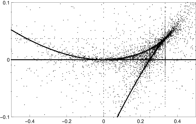
Figure 4.1. A window on $U_{4,1}({\mathbb{R}})$, which is the complement of the two discriminantal curves in the $u$-$v$ plane. Points are part of the specialization set ${\mbox{\sc U}}_{4,1}({\mathbb{Z}}[1/30])$, which applies in §2. For §5, §7, and §8, specialization sets ${\mbox{\sc U}}_{3,1,1}({\mathbb{Z}}[1/6])$, ${\mbox{\sc U}}_{3,1,1}({\mathbb{Z}}[1/6])$, and ${\mbox{\sc U}}_{4,1}({\mathbb{Z}}[1/42])$ are respectively used, and the corresponding pictures would have the same discriminant locus but different specialization points.

Let $\mathcal{P}$ be a finite set of primes with product $N$. Let ${\mathbb{Z}}[1/\mathcal{P}]={\mathbb{Z}}[1/N]$ be the ring obtained from ${\mathbb{Z}}$ by inverting the primes in $\mathcal{P}$. When the last three entries of $\nu$ are all $1$ then ${\mbox{\sc U}}_{\nu}$ is naturally a scheme over ${\mathbb{Z}}$. Accordingly it makes sense to consider ${\mbox{\sc U}}_{\nu}(R)$ for any commutative ring. The finite set of points ${\mbox{\sc U}}_{\nu}({\mathbb{Z}}[1/\mathcal{P}])$ is studied in detail in [18], including complete identifications for many $(\nu,\mathcal{P})$. For general $\nu$, one similarly has a finite subset ${\mbox{\sc U}}_{\nu}({\mathbb{Z}}[1/\mathcal{P}])$ of ${\mbox{\sc U}}_{\nu}({\mathbb{Q}})$. Its key property for us is that

(4.1) for any Hurwitz cover $${\mbox{\sc X}}_{h}\rightarrow{\mbox{\sc U}}_{\nu} u\in{\mbox{\sc U}}_{\nu}({\mathbb{Z}}[1/\mathcal{P}]) K_{h,u} \mathcal{P}_{h}\cup\mathcal{P}$$ and any , the algebra is ramified within .

In §6.5 we take $\mathcal{P}$ strictly containing $\mathcal{P}_{h}$ so as to provide examples of ramification known a priori to be tame. Otherwise, we are always taking $\mathcal{P}=\mathcal{P}_{h}$ in this paper. Figure 4.1 shows the 8461 of the known $11031$ points of ${\mbox{\sc U}}_{4,1}({\mathbb{Z}}[1/30])$ which fit into the window.

In our Hurwitz parameter formalism, we are emphasizing the multiplicity vector $\nu$ because of the following important point. Fix $r$ and a non-empty finite set of primes $\mathcal{P}$, and consider all multiplicity vectors $\nu$ with total $r$. Then ${\mbox{\sc U}}_{\nu}({\mathbb{Z}}[1/\mathcal{P}])$ tends to get larger as $\nu$ moves from $(1^{r})$ to $(r)$. This phenomenon is represented by the two cases considered for $\mathcal{P}=\{2,3,5\}$ in this paper: $|{\mbox{\sc U}}_{2,1,1,1}({\mathbb{Z}}[1/30])|=2947$, from [18, §8.5], and $|{\mbox{\sc U}}_{4,1}({\mathbb{Z}}[1/30])|\geq 11031$. In fact, as $r$ increases the cardinality $|{\mbox{\sc U}}_{1^{r}}({\mathbb{Z}}[1/\mathcal{P}])|$ eventually becomes zero [18, §2.4] while $|{\mbox{\sc U}}_{r-3,1,1,1}({\mathbb{Z}}[1/\mathcal{P}])|$ increases without bound [18, §7]. This increase is critical in supporting Conjecture 1.1.

In both Figure 4.1 and the similar Figure 6.1, one can see specialization points from ${\mbox{\sc U}}_{\nu}({\mathbb{Z}}[1/30])$ concentrating on certain lines. These lines, and other less visible curves, have the property that they intersect the discriminant locus in the projective plane exactly three times. While the polynomial $f_{25}(u,v,x)$ of §2.4 was too complicated to print, variants over any of these curves are much simpler. For example, the most prominent of the lines is $u=1/3$. Parametrizing this line by $v=(j-1)/27j$, one has the simple equation

$$f_{25}(j,x)=2^{2}(x+2)\cdot$$

$$\left(729x^{8}-486x^{7}-702x^{6}-8x^{5}+105x^{4}+1118x^{3}-1557x^{2}+1296x-576\right)^{3}$$

$$\qquad+5^{15}j(x-1)^{4}x^{9}.$$

The ramification partitions above $0$, $1$, and $\infty$ are respectively $3^{8}1$, $2^{10}1^{5}$, and $(12,9,4)$. A systematic treatment of these special curves in the cases $\nu=(3,1,1)$ and $\nu=(3,2)$ is given in [17, §7]. For general $\nu$, they play an important role in [15]. In this paper the above line $v=1/3$ will play a prominent role in §8, and analogous lines for $\nu=(2,1,1,1)$ will enter in §6.2 and §9.3.

4.3. Pairwise distinctness

For each of the $11031$ algebras $K_{u,v}$ of §2.5, and each prime $p\geq 7$, one has a Frobenius partition $\alpha_{u,v,p}$ giving the degrees of the factor fields of $K_{u,v}\otimes{\mathbb{Q}}_{p}$. For $p=7$, $11$, $13$, $17$, $19$, and $23$, the number of partitions of $25$ arising is $71$, $126$, $157$, $205$, $243$, and $302$. Taking now $p=7$, $11$, $13$, $17$, $19$, and $23$ as cutoffs, the number of tuples $(\alpha_{u,v,7},\dots,\alpha_{u,v,p})$ arising is $71$, $2992$, $10252$, $10981$, $11027$, and $11031$. Thus the $11031$ algebras are pairwise non-isomorphic. There are many other quick ways of seeing this pairwise distinctness. For example, one could use that $6772$ different discriminants $D_{u,v}$ arise as a starting point.

Abstracting this simple observation to a general Hurwitz map ${\mbox{\sc X}}_{h}\rightarrow{\mbox{\sc U}}_{\nu}$ gives

Principle A. For almost all pairs of distinct elements $u_{1}$, $u_{2}$ in ${\mbox{\sc U}}_{\nu}({\mathbb{Z}}[1/\mathcal{P}])$, the algebras $K_{h,u_{1}}$ and $K_{h,u_{2}}$ are non-isomorphic.

So, at least when one restricts to the known $11031$ elements of ${\mbox{\sc U}}_{4,1}({\mathbb{Z}}[1/30])$, Principle A holds without exception for our introductory family.

4.4. Minimal Galois group drop

The Galois group of $f_{25}(u,v,x)$ over ${\mathbb{Q}}(u,v)$ is $S_{25}$. Some of the $11031$ specialized algebras $K_{u,v}$ have smaller Galois groups as follows. First, in $93$ cases, there is a factorization of the form $K_{u,v}=K_{u,v}^{\prime}\times{\mathbb{Q}}$, with $K_{u,v}^{\prime}$ a field. Second, the discriminant of the specializing polynomial $\tau(u,v,t)$ and the discriminant of the degree twenty-five algebra $K_{u,v}$ agree modulo squares. Thus one knows the total number of times that a given discriminant class $d\in{\mathbb{Q}}^{\times}/{\mathbb{Q}}^{\times 2}$ occurs, even without inspecting the $K_{u,v}$ themselves. The number of degree $m$ fields obtained with discriminant class $d$ is as follows:

$${\begin{array}[]{r|rrrrrrrrrrrrrrrr}&-30&-15&-10&-6&-5&-3&-2&-1&1&2&3&5&6&10&15&30\\ \hline\cr 25&1050&547&310&363&641&1702&1000&480&557&360&576&572&1026&787&897&70\\ 24&14&3&2&4&5&15&8&4&2&4&10&6&3&1&12&0\end{array}.}$$

Galois groups are as large as possible given the above considerations. Thus $A_{25}$ and $A_{24}$ occur respectively $557$ times and twice, leaving $S_{25}$ and $S_{24}$ occurring respectively $10381$ and $91$ times.

To state a principle for general $h=(G,C,\nu)$, let $\mbox{\rm Gal}_{h}$ be the generic Galois group of the cover ${\mbox{\sc X}}_{h}\rightarrow{\mbox{\sc U}}_{\nu}$.

Principle B. For almost all elements $u$ in ${\mbox{\sc U}}_{\nu}({\mathbb{Z}}[1/\mathcal{P}])$, the specialized Galois group $\mbox{\rm Gal}(K_{h,u})$ contains the derived group $\mbox{\rm Gal}^{\prime}_{h}$ of the generic Galois group.

The most important case of this principle for us is when ${\mbox{\sc X}}_{h}\rightarrow{\mbox{\sc U}}_{\nu}$ is full, i.e. all of $A_{m}$ or $S_{m}$. Then the principle says that $K_{h,u}$ is full for almost all $u\in{\mbox{\sc U}}_{\nu}({\mathbb{Z}}[1/\mathcal{P}])$. In our example, $93$ of the $11031$ known points of ${\mbox{\sc U}}_{4,1}({\mathbb{Z}}[1/30])$, thus slightly less than $1\%$, are exceptions to the principle. However, these exceptions are relatively minor, in that they produce contributors to $F_{\{2,3,5\}}(24)$ rather than $F_{\{2,3,5\}}(25)$.

Principle B is formulated so that it includes other cases of interest to Conjecture 1.1. For example, let $m=m_{1}+m_{2}$ with $m_{1},m_{2}\geq 3$. Suppose $\mbox{\rm Gal}_{h}$ is one of the five intransitive groups containing $A_{m_{1}}\times A_{m_{2}}$. Then Principle B holds for $u$ if and only if $K_{h,u}$ factors as a product of two full fields. This case is illustrated many times in [15], with splittings of the form $25=10+15$ and $70=30+40$ being presented in detail in §7.1 and §7.2 respectively.

4.5. Wild ramification.

Consider the discriminants $\mbox{disc}(K_{u,v})=\pm 2^{a}3^{b}5^{c}$ as $(u,v)$ varies over the 11031 known elements of ${\mbox{\sc U}}_{4,1}({\mathbb{Z}}[1/30])$. The left part of Figure 4.2 gives the distribution of the exponents $a$, $b$ and $c$. There is much less variation in the exponents than is allowed for field discriminants of degree twenty-five algebras in general. For general algebras, the minimum value for $a$, $b$, and $c$ is of course $0$ in each case. The maximum values occur for the algebras defined by $(x^{16}-2)(x^{8}-2)x$, $(x^{18}-3)(x^{6}-3)x$, and $x^{25}-5$, and are respectively $110$, $64$, and $74$. The average values in our family are $(\langle a\rangle,\langle b\rangle,\langle c\rangle)\approx(56,43,42)$.

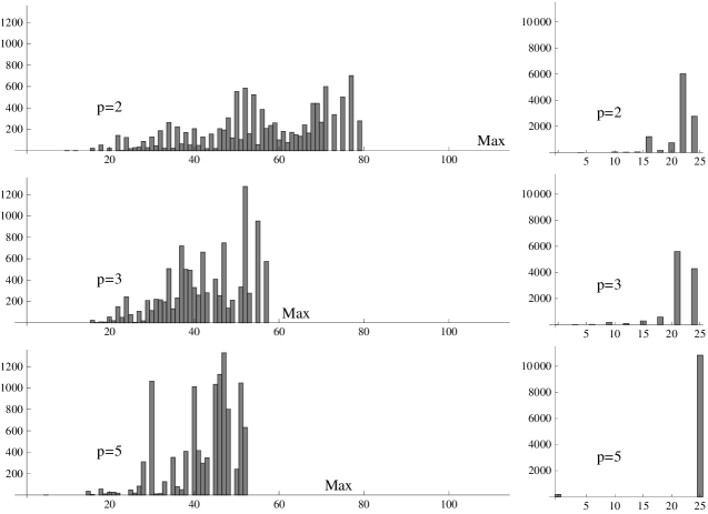
Figure 4.2. Left: distribution of the discriminant exponents ${\rm ord}_{p}(D)$ the 11031 algebras $K_{u,v}$; the variation of ${\rm ord}_{p}(D)$ is much less than is allowed by general discriminant bounds. Right: distribution of the wildness degrees $m_{p{\rm\mbox{-}wild}}$ relevant for Principle C.

There are many open questions to pursue with regard to wild ramification. One could ask for lower bounds valid for all $u$, upper bounds valid for all $u$, or even exact formulas for wild ramification as a function of $u$. Principle C is in the spirit of lower bounds:

Principle C. For almost all $u\in{\mbox{\sc U}}_{\nu}({\mathbb{Z}}[1/\mathcal{P}])$, the specialized algebra $K_{h,u}$ is wildly ramified at all primes $p\in\mathcal{P}_{h}$.

An interesting complement to Principle C is a general upper bound: $K_{h,u}$ can be wildly ramified at $p$ only if $p\in\mathcal{P}_{h}$ or $p\leq\max(\nu_{i})$.

Certainly if ${\rm ord}_{p}(K_{h,u})\geq m$ then Principle C holds for $K_{h,u}$ and $p$. The left part of Figure 4.2 shows that, for each $p$, most $K_{u,v}$ satisfy this sufficient criterion. In fact, for $p=2$, $3$, and $5$, there are only 374, 568, and 179 algebras $K_{u,v}$ which do not. However to conform to Principle C at $p$, an algebra $K_{h,u}$ needs only to satisfy a much weaker condition. Define the wild degree of a $p$-adic algebra $K$ to be the sum of the degrees of its wildly ramified factor fields. Thus in (2.3) these degrees $m_{p\rm{\mbox{-}wild}}$ for $p=2$, $3$, and $5$ are $16$, $15$, and $25$ respectively. Then conformity to Principle C at $p$ means simply that the $p$-adic wild degree is positive.

The right part of Figure 4.2 gives the distribution of $m_{p\rm{\mbox{-}wild}}$. In the cases $p=2$, $3$, and $5$, the heights of the bars above multiples of $p$ are

$$(0,0,2,0,0,45,20,44,1211,161,746,6029,2773),$$

$$(0,4,12,164,95,284,585,5598,4289),$$

$$(179,0,0,0,0,10852).$$

Thus all 11031 algebras are wild at $2$ and $3$, most having $m_{p\rm{\mbox{-}wild}}$ near its maximum possible value of $24$. For $p=5$, there are $179$ exceptions to Principle C, including all the 93 factorizing algebras. Besides these exceptions, all algebras have $m_{5\rm{\mbox{-}wild}}$ at its maximum possible value of $25$.

4.6. Expectations

As discussed in [19, §8], the Hilbert irreducibility theorem already points in the direction of Principles A and B. In a wide variety of contexts, analogs of these principles hold with great strength. For example, in [14, §9] several covers are discussed in the setting $\mathcal{P}=\{2,3\}$ and for most of them both Principles A and B hold without exception. However the situation we are considering here, with fixed $\mathcal{P}$ and arbitrarily large degree $m$, is outside the realm of previous experience. Explicitly verifying the principles in degrees large enough to contradict the mass heuristic is important for being confident that these standard expectations do indeed hold in this new realm.

We are confident that for a given $G$ and varying $h=(G,C,\nu)$, one has strict inclusion $\mathcal{P}_{h}\subset\mathcal{P}_{G}$ for only finitely many $(C,\nu)$. This expectation, together with Principle C, suggests that there are only finitely many full fields $K_{h,u}$ ramified strictly within $\mathcal{P}_{G}$. One possibility is that full number fields coming from Hurwitz-like constructions are the main source of outliers to the mass heuristic. If one believes this, then one is led to the first of the two extreme possible complements to Conjecture 1.1 discussed at the end of [19]: The sequence $F_{\mathcal{P}}(m)$ always has support on a density zero set, and it is eventually zero unless $\mathcal{P}$ contains the set of primes divisors of the order of a nonabelian finite simple group. Our verification that Principle C holds with great strength in our examples is supportive of this very speculative assertion.

5. A degree 9 family: comparison with complete number field tables

This section begins our sequence of six sample families of increasing degree. To start in very low degree, we take $G$ solvable. The number fields coming from this first example are not full and so not directly relevant to Conjecture 1.1. This family is nonetheless a good place to begin our presentation of examples, as the low degree makes comparison with complete tables of number fields possible.

5.1. A Hurwitz parameter with solvable $G$

Consider first the Hurwitz parameter $h^{\prime}=(S_{6},(21111,222,33),(3,1,1))$. The mass formula (3.6) yields $\overline{m}_{h^{\prime}}=9$. In the language of [19, §3], $S_{6}$ has nine orbits on $\mathcal{G}_{h^{\prime}}$. However none of the tuples $(g_{1},\dots,g_{5})\in\mathcal{G}_{h^{\prime}}$ generate $S_{6}$.

To place this degenerate situation into our formalism, let $G$ be the wreath product $S_{3}\wr S_{2}$ of order $72$, considered as a subgroup of $S_{6}$. The group $G$ has unique conjugacy classes with cycle type $21111$, $222$, and $33$. In place of $h^{\prime}$, take $h=(G,(21111,222,33),(3,1,1))$. This parameter accounts for everything, as $\overline{m}_{h}=m_{h}=9$.

5.2. A two-parameter polynomial.

In the present context of $\nu=(3,1,1)$, our normalized specialization polynomials take the form

$$\tau(u,v,t)=(t^{3}+t^{2}+ut+v)t.$$

The discriminant of the cubic factor is $d=4u^{3}-u^{2}-18uv+27v^{2}+4v$ from (3.5). A nonic polynomial capturing the family and a resolvent octic are as follows:

$$f_{9}(u,v,x) = x^{9}-3x^{8}+12ux^{7}-4(u+12v)x^{6}+42vx^{5}-6(4u+1)vx^{4}$$

$$\qquad+4v(2u+3v)x^{3}-12v^{2}x^{2}+3(4u-1)v^{2}x-v^{2}(4u-8v-1),$$

$$f_{8}(u,v,x) = x^{8}+x^{4}\left(18v-6u^{2}\right)+x^{2}\left(8u^{3}-36uv+108v^{2}\right)$$

$$\qquad+(-3u^{4}+18u^{2}v-27v^{2}).$$

Here $f_{9}(u,v,x)$ and $f_{8}(u,v,x)$ respectively have Galois group $9T26={\mathbb{F}}_{3}^{2}.GL_{2}({\mathbb{F}}_{3})$ and $8T23=GL_{2}({\mathbb{F}}_{3})=\tilde{S}_{4}$. Because of the complete lack of singletons in the partitions 222 and 33, our computation of $f_{9}(u,v,x)$ required substantial ad hoc deviations from the procedure sketched in §3.7.

The discriminants of the two polynomials are respectively

$$D_{9}(u,v) =-2^{24}3^{9}v^{10}d^{4}(27v-1)^{6}, D_{8}(u,v) =-2^{24}3^{19}v^{8}d^{4}\left(u^{2}-3v\right)^{2}.$$

In each case, the discriminant modulo squares is $-3$. Because of this constancy, the Galois groups of $f_{9}(u,v,x)$ and $f_{8}(u,v,x)$ over ${\mathbb{C}}(u,v)$ are respectively the index two subgroups $9T23={\mathbb{F}}_{3}^{2}.SL_{2}({\mathbb{F}}_{3})$ and $8T12=SL_{2}({\mathbb{F}}_{3})=\tilde{A}_{4}$. The last factor of the discriminant in each case is an artifact of our particular polynomials; these factors do not contribute to field discriminants in specializations.

5.3. Comparison of specializations with complete tables of number fields

We work with $507$ pairs $(u,v)$ in ${\mbox{\sc U}}_{3,1,1}({\mathbb{Z}}[1/6])$. Twenty-one of them have $v=1/27$ and so $f_{9}(u,v,x)$ is not separable. For forty more, $f_{9}(u,v,x)$ also reduces, with the factorization partitions $63$, $81$, $6111$, and $333$ occurring respectively $9$, $29$, $1$, and $1$ times. The remaining $446$ specialization points yield only $129$ different fields, as for example $(-13/12,2/9)$, $(11/12,1/9)$, $(-5/12,-8/27)$, $(1/4,-1/27)$, $(1/4,2/27)$, $(35/108,8/243)$, $(1/4,64/3375)$, and $(19/2028,1/59319)$ all yield the field defined by $x^{9}-9x^{7}+27x^{5}-27x^{3}-4$. Moreover, a wide variety of subgroups of $9T26$ appear, as follows.

$$\begin{array}[]{r|cccccccc}\mbox{Group $G$:}&9T4&9T8&9T12&9T13&9T16&9T18&9T19&9T26\\ \mbox{Size $|G|$:}&18&36&54&54&72&108&144&432\\ \hline\cr\mbox{Number of fields in family:}&2&1&10&1&5&20&8&82\\ \hline\cr\mbox{Total number of fields:}&4&1&12&3&5&23&8&87\end{array}$$

The last line compares with the relevant complete lists from [9]. It gives the total number of number fields with the given Galois group and with discriminant of the form $-2^{a}3^{b}$ with $a$ even and $b$ odd. One can get even a larger fraction of the total number of fields by specializing outside of ${\mbox{\sc U}}_{3,1,1}({\mathbb{Z}}[1/6])$, both by considering the curve at infinity and then by specializing also at the rare-but-existent points of say ${\mbox{\sc U}}_{3,1,1}({\mathbb{Z}}[1/6p])$, where the auxiliary prime $p$ does not divide the discriminant of the field constructed. The fact that such a large fraction of all fields of the type considered come from a single Hurwitz family is suggestive that other Hurwitz families may be essentially the only source of number fields with certain invariants.

The current family presents many examples of phenomena that Principles A, B, and C say are rare in general. The drop from $507$ specialization points to only $129$ fields constitutes many exceptions to Principle A. The further drop from $129$ fields to just $82$ fields with the generic Galois group constitutes many exceptions to Principle B. Some of the specializations are tamely ramified or even unramified at $2$, and thus correspond to exceptions to Principle C. These exceptions form the first data-point arguing for the expectation already formulated in the introduction: as the complexity of the Hurwitz family increases, the frequency of exceptions decreases.

6. A degree 52 family: tame ramification and exceptions to Principle B

In our introductory family, the only exceptions to Principle B were algebras of the form $K_{h,u}={\mathbb{Q}}\times K_{h,u}^{\prime}$ with $K_{h,u}^{\prime}$ full. In specializing many other full families, most of the exceptions to Principle B we have found have this very same form. In this section, we present a family which is remarkable because some of its specializations have a much more pronounced drop in fullness. However we do not regard this more serious failure of Principle B as anywhere near extreme enough to raise doubts about Conjecture 1.1.

6.1. A Hurwitz parameter yielding a rational ${\sf X}_{h}$

We start from the normalized Hurwitz parameter

$$h=(S_{6},(21111,222,3_{1}111,3_{\infty}2_{0}1),(2,1,1,1)).$$

All rational functions with this normalized Hurwitz parameter have the form

$$g(s)=\frac{\left(s^{3}+bs^{2}+cs+x\right)^{2}}{as^{2}(s-y)}.$$

The ramification requirement on $g$ at $1$ is that $(g(1),g^{\prime}(1),g^{\prime\prime}(1))=(1,0,0)$. These three equations let one eliminate $a$, $b$, and $c$ via

$$a =-64(x+1)^{2}(y-1)^{3},$$

$$b =4xy-3x+4y-6,$$

$$c =-8xy^{2}+12xy-6x-8y^{2}+12y-3.$$

Using a resolvent as usual, we find that the critical values of $g(s)$ besides $0$, $1$, and $\infty$ are the roots of $Wt^{2}+(V-U-W)t+U$ where

$$U =(4xy-x+3y)\left(64x^{2}y^{4}-160x^{2}y^{3}+180x^{2}y^{2}-108x^{2}y+27x^{2}+256xy^{4}\right.$$

$$\left.\;\;\;\;-736xy^{3}+864xy^{2}-540xy+162x+192y^{4}-576y^{3}+576y^{2}-216y+27\right)^{2},$$

$$V =3^{3}(2xy-x+1)^{4}\left(64xy^{3}-144xy^{2}+108xy-27x+64y^{3}-144y^{2}+81y\right),$$

$$W =2^{12}3^{3}(x+1)^{4}(y-1)^{6}y^{3}.$$

Comparing with the standard quadratic $t^{2}+(v-u-1)t+u$, one gets the rational presentation

(6.1) $$u =\frac{U}{W}, v =\frac{V}{W}.$$

Summarizing, birationally we have ${\sf X}_{h}={\mathbb{C}}_{x}\times{\mathbb{C}}_{y}$, ${\sf U}_{\nu}={\mathbb{C}}_{u}\times{\mathbb{C}}_{v}$, and the equations (6.1) give the map ${\sf X}_{h}\rightarrow{\sf U}_{\nu}$. Removing $y$ by a resolvent gives the single equation $f_{52}(u,v,x)=0$. Likewise removing $x$ by a resolvent gives the single equation $\phi_{52}(u,v,y)=0$. The left sides have $2781$ and $829$ terms respectively.

The discriminants of $f_{52}(u,v,x)$ and $\phi_{52}(u,v,y)$ are both $-3$ times a square in ${\mathbb{Q}}(u,v)$. The Galois groups of these polynomials over ${\mathbb{Q}}(u,v)$ are $S_{52}$, but over ${\mathbb{C}}(u,v)$ they reduce to $A_{52}$. This general phenomenon appeared already in the previous section. It is not of central importance to us, which is why we generally refer to full fields and only sometimes make the distinction between $S_{m}$ and $A_{m}$ fields.

6.2. Specialization to curves

Using homogeneous coordinates $U$, $V$, and $W$, related to our standard coordinates $u$ and $v$ via (6.1), we can view ${\sf U}_{2,1,1,1}$ as completed by the projective plane. Its complement in this projective plane has four components,

A:

the vertical line $U=0$,

B:

the horizontal line $V=0$,

${\sf C}$:

the line at infinity $W=0$, and

D:

the conic $U^{2}+V^{2}+W^{2}-2UV-2UW-2VW=0$.

Figure 6.1 draws A, B, and D. Note that lines A, B, and ${\sf C}$ pass through points ${\sf a}=(0:1:1)$, ${\sf b}=(1:0:1)$, and ${\sf c}=(1:1:0)$ respectively, while the conic $D$ goes around ${\sf d}=(1:1:1)$.

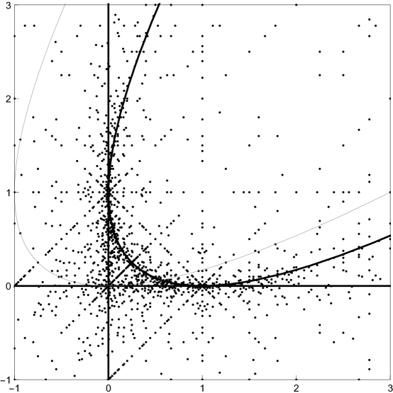
Figure 6.1. A window on ${\mbox{\sc U}}_{2,1,1,1}({\mathbb{R}})$, which is the complement of the three thick discriminantal curves in the $u$-$v$ plane. Points are part of the specialization set ${\mbox{\sc U}}_{2,1,1,1}({\mathbb{Z}}[1/30])$ which is used in both §6 and §9. The thin parabola $(u-v)^{2}=4v$ plays a role only in §6.

A general line in the projective plane intersects the discriminant locus in five points. However the lines that go through two of the points in $\{{\sf a},{\sf b},{\sf c},{\sf d}\}$ intersect the discriminant locus only three times. These six lines are parametrized in Table 6.1, so that the three points become $0$, $1$, and $\infty$. Exactly as in Figure 4.1 earlier, the lines are clearly suggested by the drawn specialization points. Having used homogeneous coordinates for two paragraphs to make an $S_{3}$ symmetry clear, we now return to our standard practice of focusing on the affine $u$-$v$ plane.

When restricted to any one of the six lines, the cover ${\sf X}_{h}$ remains full. This preserved fullness is in the spirit of Principle B. Table 6.1 gives the ramification partitions of these restricted covers. Note that all partitions are even, reflecting the fact that the monodromy group is only $A_{52}$. Before beginning any computations with polynomials, we knew these partitions and the fullness of the six covers from a braid group computation.

$$\begin{array}[]{c|cc|lllc}\mbox{Line}&u&v&\lambda_{0}&\lambda_{1}&\lambda_{\infty}&\mbox{genus}\\ \hline\cr{\sf ad}&4t&1&12^{2}\;6\;4^{4}\;3\;2\;1&3^{8}\,2^{12}\,1^{4}&20\;12\;5\;4^{3}\,2\;1&6\\ {\sf bd}&1&4t&10^{2}\,8\;6^{3}\,5\;1&3^{8}\,2^{12}\,1^{4}&10^{2}\,6^{2}\,5\;4^{2}\,2^{2}\,1^{3}&5\\ {\sf cd}&t/4&t/4&4^{9}\,2^{7}\,1^{2}&3^{8}\,2^{12}\,1^{4}&6^{4}\,4^{6}\,2^{2}&0\\ {\sf bc}&t&t-1&2^{22}\;1^{8}&10^{2}\,8\;6^{3}\,5\;1&6^{4}\,4^{6}\,2^{2}&2\\ {\sf ac}&t-1&t&4^{9}\,2^{3}\,1^{10}&12^{2}\,6\;4^{4}\,3\;2\;1&6^{4}\,4^{6}\,2^{2}&5\\ {\sf ab}&t&1-t&12^{2}\,6\;4^{4}\,3\;2\;1&10^{2}\,8\;6^{3}\,5\;1&5^{5}\,4^{2}\,3^{4}\,1^{7}&9\\ \end{array}$$

Table 6.1. Six lines in ${\sf U}_{2,1,1,1}$ and topological information on their preimages in ${\sf X}_{h}$.

To give an explicit degree $52$ polynomial coming from the cover ${\sf X}_{h}\rightarrow{\sf U}_{2,1,1,1}$, we work over the line ${\sf c}{\sf d}$. The preimage of ${\sf cd}$ is a curve in the $x$-$y$ plane with equation having $x$-degree 3, $y$-degree 6, and twenty-two terms. A parametrization is

$$x =-\frac{\left(s^{2}-2s-2\right)\left(s^{4}-4s^{3}+4s+2\right)}{2s^{3}}, y =-\frac{3\left(s^{2}-2s-2\right)}{2(s-2)\left(s^{2}-4s-2\right)}.$$

Using the domain coordinate $s$ and the target coordinate $t$, the restricted rational function takes the form

(6.2) $$t=\frac{-A}{C}=\frac{B}{C}+1.$$

Here $A$, $B$, and $C$ sum to zero and are given explicitly by

$$A = (s+1)^{4}\left(s^{8}-10s^{7}+34s^{6}-40s^{5}-2s^{4}+8s^{3}+8s^{2}+16s+8\right)^{4}$$

$$\qquad(s-2)^{2}\left(s^{2}-4s-2\right)^{2}\left(s^{4}-6s^{3}+9s^{2}-6\right)^{2}(s-4)s,$$

$$B = -\left(s^{8}-12s^{7}+52s^{6}-92s^{5}+30s^{4}+96s^{3}-72s^{2}-48s+8\right)^{3}$$

$$\qquad\left(s^{12}-12s^{11}+48s^{10}-52s^{9}-87s^{8}+108s^{7}+264s^{6}-216s^{5}\right.$$

$$\qquad\left.-312s^{4}+48s^{3}+192s^{2}+96s+16\right)^{2}\left(s^{4}-4s^{3}+4s+2\right),$$

$$C = 2^{2}\left(2s^{3}-9s^{2}+6s+2\right)^{6}\left(s^{6}-6s^{5}+6s^{4}+10s^{3}-6s^{2}-12s-4\right)^{4}$$

$$\qquad\left(s^{2}-2s-2\right)^{2}.$$

This explicit slice is intended to give a sense of the full cover for $h_{52}$, just as the slices in §4.2 and §8.2 indicate the covers for $h_{25}$ and $h^{*}_{96}$ respectively. Here we have explicitly presented information at all three of the cusps, not just at $0$ and $\infty$ as in §4.2 and §8.2.

6.3. No exceptions to Principles A and C

Unlike all our previous examples, the current $\nu$ contains at least three ones. It thus fits into the framework of [18], where many ${\mbox{\sc U}}_{\nu}({\mathbb{Z}}[1/\mathcal{P}])$ for such $\nu$ are completely identified. We therefore can be more definitive in reporting specialization results.

The set ${\mbox{\sc U}}_{2,1,1,1}({\mathbb{Z}}[1/30])$ contains exactly $2947$ points [18, §8.5] and is drawn in Figure 6.1. The Hurwitz number algebras $K_{h,u}$ are all non-isomorphic, so that Principle A holds without exception. All $2947$ algebras are wildly ramified at all three of $2$, $3$, and $5$, so that Principle C also holds without exception; in fact ${\rm ord}_{p}(D)\geq 52$ fails at $p=2$, $3$, and $5$ only $0$, $60$, and $481$ times, so the verification of Principle C is particularly easy at $p=2$.

6.4. Easily explained exceptions to Principle B

Twenty-five of the 2947 specialization points $(u,v)$ give exceptions to Principle B. Three of these, namely $(3/8,1/8)$, $(1/16,-375/16)$, $(16,-375)$ are exceptions of the sort we have seen earlier: $K_{h,u}={\mathbb{Q}}\times K_{h,u}^{\prime}$ with $K_{h,u}^{\prime}$ full. Exceptions of this nature are not surprising whenever the Hurwitz cover is rational. In this case the three points in question come respectively from points $(-1/6,3/8)$, $(-4/3,3/4)$, and $(-3,3/4)$ in ${\mbox{\sc X}}_{h}({\mathbb{Q}})$.

In fact, any point $(x,y)\in{\mbox{\sc X}}_{h}({\mathbb{Q}})$ causes such a factorization, but typically its image $(u,v)$ causes ramification at extraneous primes. For example, take $s=1$ in (6.2), making

(6.3) $$t=\frac{111936400}{43923}=\frac{2^{4}\,5^{2}\,23^{4}}{3\;11^{4}}=1+\frac{37^{3}\,47^{2}}{3\;11^{4}}.$$

The number field $K^{\prime}$ defined by the degree $51$ factor of $f_{52}(t,s)$ has discriminant $-2^{102}3^{95}5^{48}11^{16}37^{12}47^{16}$. Whenever we discuss exceptions to Principle B, we always have in mind a fixed $\mathcal{P}$, here $\{2,3,5\}$, and do not consider fields like $K^{\prime}$ to be exceptions.

6.5. Ramification at tame primes

Recall from §4.5 that ramification at $p$ in a Hurwitz number algebra $K_{h,u}$ can only be wild if $p\in\mathcal{P}_{h}$ or $p\leq\max_{i}\nu_{i}$. The field $K^{\prime}$ from the previous subsection presents a convenient opportunity to illustrate how ramification in $K_{h,u}$ at the remaining primes is calculable in purely group-theoretic terms.

To describe the factorization of the local algebras $K_{p}^{\prime}$, we represent the fields appearing by symbols $e_{c}^{f}$ as in (2.3). We simplify by just writing $e^{f}$ for tame fields, since tameness implies $c=e-1$. The factorizations are

2: $$\;{\bf 16}_{38}\,{\bf 16}_{38}\,{\bf 8}_{16}\,{\bf 2}_{3}\,{\bf 2}_{3}\,{\bf 2}_{2}\,{\bf 2}_{2}\,1^{2}\,1,\;\;\;\;\;\;\;\;\;\; \;3^{6}\,3^{2}\,1^{16}\,1^{2}\,1^{2}\,1^{2}\,1^{2}\,1\;1\;1 \rightarrow 3^{8}1^{27},$$ 11:

3: $$\;{\bf 18}_{39}\,{\bf 12}_{21}^{2}\,{\bf 6}_{11}\;{\bf 3}_{3}, \;2^{5}\,2^{4}\,2^{2}\,2\;1^{18}\,1^{3}\,1\;1\;1\;1\;1\;1 \rightarrow 2^{12}1^{27},$$ 37:

5: $$\;{\bf 25}_{40}\,2^{4}\,2^{4}\,1^{4}\,1^{2}\,1\;1\;1\;1, \;3^{6}\,3^{2}\,1^{4}\,1^{4}\,1^{4}\,1^{4}\,1^{4}\,1^{2}\,1 \rightarrow 3^{8}1^{27}.$$ 47:

The wild primes behave in a complicated way as always, with $p$-wildness at $p=2$, $3$, and $5$ being $48$, $51$, and $25$. However the tame primes are much more simply behaved.

To work at an even simpler level, we factor over the maximal unramified extension of ${\mathbb{Q}}_{p}$, rather than ${\mathbb{Q}}_{p}$ itself. For tame primes, this corresponds to regarding the printed exponents $f$ simply as multiplicities, and collecting together symbols with a common base. The resulting tame ramification partitions are indicated to the right, after arrows.

Note that there are actually four primes greater than $5$ involved in (6.3). With their naturally occurring exponents, $11^{4}$ is associated to $\infty$, $23^{4}$ to $0$, and $37^{3}$ and $47^{2}$ to $1$. In general, tame ramification partitions can be computed from the placement of the specialization point in ${\mbox{\sc U}}_{\nu}({\mathbb{Q}}_{p})$ and braid group considerations. In the setting of three-point covers, the general formula is simple, and uses the standard notion of the power of a partition. Namely, if $p^{m}$ is associated to $\tau\in\{0,1,\infty\}$ its tame ramification is the power $\lambda^{m}_{\tau}$ of the geometric ramification partition $\lambda_{\tau}$. Applying the ${\sf cd}$ line of Table 6.1, the partitions $\lambda_{\infty}^{4}=3^{8}1^{27}$, $\lambda_{0}^{4}=1^{51}$, $\lambda_{1}^{3}=2^{12}1^{27}$, and $\lambda_{1}^{2}=3^{8}1^{27}$ do indeed agree with the partitions found by direct factorization of the polynomial defining $K^{\prime}$.

The mass heuristic reviewed in §1.1 is based on an equidistribution principle. In the horizontal direction, it translates to the following conjecture, proved for $m\leq 5$: when one considers full degree $m$ fields ordered by their absolute discriminant outside of $p$, all tame ramification partitions are asymptotically equally likely. We regard the fact that Hurwitz number fields escape the mass heuristic as being directly related to their highly structured ramification. In the current instance, there are $239,943$ partitions of the integer $51$, and the two partitions $2^{12}1^{27}$ and $3^{8}1^{27}$ are far from typical.

6.6. A curve of more extreme exceptions to Principle B

The twenty-two exceptions not discussed in §6.4 all have a common geometric source: above the base curve B given by $(u-v)^{2}=4v$, the cover splits into a full degree $42$ cover of genus five and a full degree $10$ cover C of genus zero. While decompositions $52=51+1$ are governed by rational points on ${\mbox{\sc X}}_{h}$ itself, decompositions of the form $52=42+10$ are governed by rational points on a resolvent variety of degree $\binom{52}{10}$ over ${\mbox{\sc U}}_{2,1,1,1}$. As this degree is about 15 billion, the existence of a entire curve of rational points is remarkable.

To reveal the structure of the cover ${\mbox{\sc C}}\rightarrow{\mbox{\sc B}}$, we parametrize the base curve B via

(6.4) $$u =\frac{4t}{(t-1)^{2}}, v =\frac{4}{(t-1)^{2}}.$$

In the decompositions $K_{h,(u,v)}=K^{42}_{t}\times K_{t}$, the twenty-two $K^{42}_{t}$ are all full degree forty-two fields, with pairwise distinct discriminants.

The genus zero curve C is given by $x(4y-3)^{3}=-24y^{2}(2y-3)$, and so $y$ is a parameter. The map from the $y$-line C to the $t$-line B is given by the vanishing of

$$f_{10}(t,y) = (4y-3)(8y-3)\left(32y^{4}-192y^{3}+360y^{2}-252y+27\right)^{2}$$

$$\qquad\;\,+t(4y-9)\left(96y^{4}-256y^{3}+216y^{2}-108y+27\right)^{2}.$$

Thus one has two visible ramification partitions $\lambda_{0}=\lambda_{\infty}=222211$. The discriminant of $f_{10}(t,y)$ is $-2^{136}3^{57}5^{25}t^{4}(t-1)^{5}(t-9)^{5}$. At the other singular values, the ramification partitions are $\lambda_{1}=\lambda_{9}=32221$. In fact, the decic algebras $K_{t}$ and $K_{9/t}$ are isomorphic via the involution $y\mapsto(6y-9)/(8y-6)$.

At the level of the decic cover only, we have just indicated a failure of Principle A: rather than $22$ distinct decic algebras, there are ten pairs switched by $t\leftrightarrow 9/t$ and then two algebras $K_{3}$ and $K_{-3}$ arising once each. The ten algebras arising twice are all full fields and wildly ramified at all three of $2$, $3$, and $5$. However $K_{3}$ and $K_{-3}$ are not full, and not wildly ramified at $5$, giving failures of Principle B and C at this decic cover level.

In terms of supporting Conjecture 1.1 for $\mathcal{P}=\{2,3,5\}$, the exceptional behavior above B is in a sense good. Instead of twenty-two contributions to $F_{\mathcal{P}}(52)$, one gets twenty-two contributions to $F_{\mathcal{P}}(42)$ and then ten more to $F_{\mathcal{P}}(10)$. But in another sense this exceptional behavior is bad. It explicitly illustrates phenomena which, if occurring ubiquitously in high degree, might make Conjecture 1.1 false. However our computations suggest that, far from becoming ubiquitous, the phenomena exhibited here become rarer as degrees increase.

7. A degree $60$ family: non-full monodromy and a prime drop

The statement of Conjecture 1.1 involves all finite nonabelian simple groups equally. In this paper, however, we are focusing on the simple groups $A_{5}$ and $A_{6}$ because of the computational accessibility of the corresponding families ${\sf X}_{h}\rightarrow{\sf U}_{\nu}$. In this section and the next, we add some balance by presenting results on covers coming from simple groups not of the form $A_{n}$. The family presented here has the particular interest that it is non-generic in two ways.

7.1. A Hurwitz parameter with unexpectedly non-full monodromy

The simple group $G=PSL_{3}({\mathbb{F}}_{3})$ has order $5616=2^{4}\cdot 3^{3}\cdot 13$ and outer automorphism group of order two. It has two non-isomorphic degree $13$ transitive permutation representations, coming from an action on a projective plane ${\mathbb{P}}^{2}({\mathbb{F}}_{3})$ and its dual $\widehat{{\mathbb{P}}}^{2}({\mathbb{F}}_{3})$. These actions are interchanged by the outer involution. The two smallest non-identity conjugacy classes in $G$ consist of order $2$ and order $3$ elements. In each of the degree $13$ permutation representations, these elements act with cycle structure $2^{4}1^{5}$ and $3^{3}1^{4}$ respectively.

Let $h=(PSL_{3}({\mathbb{F}}_{3}),(2^{4}1^{5},3^{3}1^{4}),(3,2))$. To conform to our main reference [11] for this section, we make a quadratic base change and work over ${\sf U}_{3,1,1}$ rather than ${\sf U}_{3,2}$. A braid group computation reveals that the degree $120$ Hurwitz cover $\pi_{h}$ factors as a composition of three covers as indicated:

(7.1) $${\sf X}_{h}\stackrel{{\scriptstyle 2}}{{\rightarrow}}{\sf X}^{*}_{h}\stackrel{{\scriptstyle 15}}{{\rightarrow}}{\sf Quart}\stackrel{{\scriptstyle 4}}{{\rightarrow}}{\sf U}_{3,1,1}.$$

The intermediate cover ${\sf X}^{*}_{h}$ is just the quotient of ${\sf X}_{h}$ by the natural action of $\mathrm{Out}(G)$. This failure of fullness illustrates one of the general phenomena treated at length in [19].

However, very unusually in comparison with Table 3.2, the reduced Hurwitz cover $\pi_{h}^{*}:{\sf X}^{*}_{h}\rightarrow{\sf U}_{3,1,1}$ is also not full. It clearly fails to be primitive, because of the intermediate cover ${\sf Quart}$. Moreover, the degree fifteen map is not even full, as its monodromy group is $S_{6}$ in a degree $15$ transitive representation.

The degree $13$ covers of the projective line parametrized by ${\sf X}_{h}$ have genus zero. Using this fact as a starting point, König [11] succeeded in finding coordinates $a$, $b$ on ${\sf X}_{h}$, with corresponding covers ${\sf P}^{1}_{s}\rightarrow{\sf P}^{1}_{t}$ being as follows. Define

$$f_{0} = \frac{abs}{3}+\frac{ab}{9}+as^{2}-\frac{a}{3}+s^{3},$$

$$f_{1} = \frac{s^{2}\left(ab^{2}-4ab+12a-3b^{2}-9\right)}{(b-3)^{2}}+\frac{s\left(ab^{2}-4ab+12a-9b-9\right)}{3(b-3)}+s^{3}-1,$$

$$g_{0} = \frac{abs}{3}+\frac{ab}{9}+as^{2}-\frac{a}{3}+s^{3},$$

$$g_{1} = \frac{1}{9}s\left(4ab^{2}-6ab+9a+9b-27\right)+\frac{1}{3}s^{2}(4ab-3a+9)+as^{3}-a.$$

Then the two-parameter family is given by $g(a,b,t,s):=f_{0}^{3}f_{1}s-tg_{0}^{3}g_{1}=0$.

König’s interest in this family is in producing number fields with Galois group $G$. For example $(a,b,t)=(-9,-6,-3)$ gives a totally real such field with discriminant $3^{12}251^{4}353^{4}$. To systematically study specializations, it is important to determine the discriminant of $g(a,b,t,s)$. Computation shows that it has the following form:

$$D(a,b,t) =\left(-\frac{4}{3}ab^{3}+a^{2}b^{2}+6ab^{2}-3b^{2}-4a^{2}b-18ab+18b+12a^{2}-27\right)^{28}$$

$$\qquad\qquad a^{12}(b-3)^{18}t^{6}\left(C_{0}t^{3}+C_{1}t^{2}+C_{2}t+C_{3}\right)^{4}.$$

Here $C_{0}$, $C_{1}$, $C_{2}$, and $C_{3}$ as expanded elements of ${\mathbb{Q}}[a,b]$ have $24$, $45$, $53$, and $36$ terms respectively. Because of the complicated nature of this discriminant, it is hard to get field discriminants to be as small as the one exhibited above.

For König’s purposes of constructing degree thirteen fields with Galois group $G$, he does not need the map to configuration space at all. To move over into our context of constructing Hurwitz number fields, we do need this map. Replacing $t$ in $(C_{0}t^{3}+C_{1}t^{2}+C_{2}t+C_{3})$ with $C_{1}t/C_{0}$ and setting the resulting cubic proportional to $t^{3}+t^{2}+ut+v$ gives a degree $120$ map $\pi_{h}$ from the $a$-$b$ plane ${\sf X}_{h}$ to the $u$-$v$ plane ${\sf U}_{3,1,1}$. Removing $a$ from the pair of equations gives a degree $120$ polynomial $f_{120}(u,v,b)\in{\mathbb{Q}}(u,v)[b]$ describing the covering map.

7.2. Reduction to degree $60$

To reduce from the degree $120$ cover ${\sf X}_{h}$ to the degree $60$ cover ${\sf X}_{h}^{*}$, we proceed as follows. For $(a_{i},b_{i})\in{\mathbb{Q}}^{2}$, one gets $(u_{i},v_{i})=\pi_{h}(a_{i},b_{i})\in{\mathbb{Q}}^{2}$. Then $f_{120}(u_{i},v_{i},b)\in{\mathbb{Q}}[b]$ factors. For almost all choices of $(a_{i},b_{i})$, the degrees of the irreducible factors are $90$, $6$, $6$, $4$, $4$, $4$, $4$, $1$, and $1$. One of the linear factors is $b-b_{i}$ and we write the other one as $b-b_{i}^{\prime}$. Then typically just one rational number $a_{i}^{\prime}$ satisfies the two equations $\pi_{h}(a^{\prime}_{i},b_{i}^{\prime})=(u_{i},v_{i})$. From enough datapoints we interpolate to get the canonical involution on ${\sf X}_{h}$. It is

(7.2) $$a^{\prime} =\frac{(b-3)(4ab+6a+9)}{ab^{2}-4ab+12a-18b+18}, b^{\prime} =\frac{3b}{b-3}.$$

This involution is useful even in König’s context. For example, specializing at $(a^{\prime},b^{\prime},t)=(171/58,2,-3)$ gives the dual totally real number field, also with discriminant $3^{12}251^{4}353^{4}$.

A quantity stabilized by the involution is $x=b^{2}/(b-3)$. The resolvent

$$\mbox{Res}_{b}(f_{120}(u,v,b),(b-3)x-b^{2})$$

is proportional the square of degree $60$ polynomial $f_{60}(u,v,x)$. This polynomial captures the cover ${\sf X}_{h}^{*}\rightarrow{\sf U}_{3,1,1}$.

7.3. Low degree resolvents

From the braid group computation, we know that the monodromy group has quotients of type $S_{3}$, $S_{4}$, and $8T40=2^{3}.S_{4}$. Here the $S_{4}$ quotient corresponds to the cover ${\sf Quart}$. Equations for these quotients and their discriminants are

$$f_{3}(u,v,x) =x^{3}+x^{2}+xu+v, D_{3} =d,$$

$$f_{4}(u,v,x) =x^{4}-2x^{2}v-8xv^{2}-4uv^{2}+v^{2}, D_{4} =-2^{12}dv^{6},$$

$$f_{8}(u,v,x) =x^{8}+8x^{4}duv-72x^{4}dv^{2} D_{8} =-2^{60}d^{17}v^{14}\left(u^{3}-v\right)^{4}.$$

$$\qquad+64x^{2}d^{2}v^{2}-16d^{3}v^{2},$$

Here we have seen the cubic and quartic polynomials in §3.4, with $d$ being given explicitly in (3.5).

7.4. Reduction to degree $24$

The equation $f_{4}(u,v,m)=0$ is linear in $u$. Solving it gives $u=(m^{4}-2m^{2}v+v^{2}-8mv^{2})/(4v^{2})$. Expressing $f_{60}(u,v,x)$ in terms of $m$, $v$, and $x$ and factoring, one gets $g_{15}(m,v,x)g_{45}(m,v,x)$. Here $g_{15}(m,v,x)$ has Galois group $S_{6}$ over ${\mathbb{Q}}(m,v)$, in a degree $15$ permutation representation.

Abbreviate $e=m^{3}-mv-2v^{2}$. Then the polynomial for the standard sextic representation works out to

$$g_{6}(m,v,x)=2x^{6}v^{2}-3x^{4}e\left(m^{2}-v\right)-8x^{3}e^{2}-6x^{2}e^{2}m+2e^{3}.$$

Returning to the original base, one gets a degree $24$ polynomial,

$$f_{24}(u,v,x)=\mbox{Res}_{m}(f_{4}(u,v,m),g_{6}(m,v,x)).$$

Similarly, by means of the outer automorphism of $S_{6}$, one has a twin polynomial $g_{6}^{t}(m,v,x)$ and its degree $24$ polynomial $f^{t}_{24}(u,v,x)$. While $f_{60}(u,v,x)$, $f_{24}(u,v,x)$, and $f_{24}^{t}(u,v,x)$ all have the same splitting field, the latter two are much easier to work with because of their lower degree.

7.5. Specialization to number fields

We have specialized at the $507$ points in ${\mbox{\sc U}}_{3,1,1}({\mathbb{Z}}[1/6])$ considered in §5, obtaining $507$ algebras with discriminant of the form $\pm 2^{a}3^{b}$. Replacing $(u,v)$ by $(v/u^{2},v^{2}/u^{3})$, corresponding to the involution of ${\sf U}_{3,1,1}$ with quotient ${\sf U}_{3,2}$, gives an isomorphic algebra. We report on the fields involved in these algebras, since Galois groups are small enough so that future comparison with other sources of fields with these groups seems promising.

For simplicity, we exclude the twenty-three $(u,v)$ where $u=0$, so that the involution above is everywhere defined. We switch coordinates to the coordinates used in [17] via $(p,q)=(3u,3v/u^{2})$ and $(u,v)=(p/3,p^{2}q/27)$. In the new coordinates, the involution is simply $(p,q)\mapsto(q,p)$, and we normalize by requiring $p\leq q$. We then have $232$ algebras $K_{p,q}$ with $p<q$ and $20$ algebras $K_{p,p}$. Besides these algebras, we have their twins $K_{p,q}^{t}$, and their common octic and quartic resolvents $\tilde{R}_{p,q}$ and $R_{p,q}$.

Despite the non-generic behavior of the family in general, Principal A has no exceptions in the current context: the $252$ algebras $K_{p,q}$ and their $252$ twins $K_{p,q}^{t}$ form $504$ non-isomorphic algebras. Principle C also has no exceptions, as all algebras are wildly ramified at both $2$ and $3$.

There are many exceptions to Principle B. For example $K_{153/1849,129/289}$ factors as $6+6+12$ with the factors having Galois group $6T9$, $6T15=A_{6}$, and $12T299=S_{6}\wr S_{2}$. Its twin factors as $3+3+6+12$ with factors having Galois groups $S_{3}$, $S_{3}$, $A_{6}$, and $S_{6}\wr S_{2}$. The two $A_{6}$ factors are given by the polynomials

(7.3) $$f_{6}(x) = x^{6}-3x^{5}+3x^{4}-6x^{2}+6x-2,$$

(7.4) $$f^{t}_{6}(x) = x^{6}-3x^{4}-12x^{3}-9x^{2}+1.$$

These polynomials will be discussed further at the end of the next subsection.

For the rest of this section, we avoid Galois-theoretic complications like those of the last paragraph by requiring that $R_{p,q}$ either has an irreducible cubic factor or is irreducible itself. There are 39 $(p,q)$ of the first type, and 178 $(p,q)$ of the second. Failures of Principle B in this restricted setting are very mild, as $A_{6}^{4}$ is a subgroup of the Galois group of all these specializations. In the case of a cubic-times-linear quartic resolvent, we change notation by focusing on the larger degree part, so that $K_{p,q}$, $K_{p,q}^{t}$, $\tilde{R}_{p,q}$, and $R_{p,q}$ now have degrees $18$, $18$, $6$, and $3$.

7.6. Some lightly ramified number fields

Table 7.1 summarizes the fields under consideration, with resolvent Galois groups indicated by $Q$ and $\tilde{Q}$. In all cases, if $K_{p,q}$ has some Galois group $mTj$ then its twin $K_{p,q}^{t}$ has the same Galois group $mTj$. For each Galois group, the table gives a corresponding field in our collection with smallest root discriminant. Thus $(p,q)$ is chosen because one of $\delta=\mbox{rd}(K_{p,q})$ and $\delta^{t}=\mbox{rd}(K_{p,q}^{t})$ is small; the other is sometimes substantially larger. Galois groups were computed by Magma, making use thereby of the algorithms of [8] and works classifying permutation groups.

$${\begin{array}[]{crc|cc|cr|rc|rc}Q&|\tilde{Q}|&\tilde{Q}&p&q&\mbox{Gal}(K_{p,q})&\#&\lx@intercol\hfil D\hfil\lx@intercol&\delta&\lx@intercol\hfil D^{t}\hfil\lx@intercol&\delta^{t}\\ \hline\cr S_{3}&6&6T2&1/12&24&18T971&1&2^{22}3^{46}&38.66&2^{24}3^{44}&36.95\\ S_{3}&12&6T3&-3/125&1&18T972&7&2^{26}3^{41}&33.24&2^{26}3^{39}&29.42\\ A_{3}&6&6T6&9/121&11/27&18T974&3&-2^{18}3^{46}&33.14&-2^{24}3^{44}&36.95\\ S_{3}&24&6T7&-3/49&7/3&18T976&1&2^{30}3^{46}&52.60&2^{32}3^{44}&50.29\\ S_{3}&48&6T11&1/9&9&18T977&27&-2^{33}3^{41}&43.52&-2^{27}3^{39}&30.57\\ \hline\cr C_{4}&16&8T7&{18}/{25}&{5}/{6}&24T24946&2&2^{87}3^{24}&37.01&2^{97}3^{24}&49.41\\ V&16&8T9&-72&{3}/{16}&24T24948&3&2^{54}3^{40}&29.68&2^{70}3^{38}&43.00\\ V&16&8T11&-27&-{1}/{3}&24T24949&3&2^{48}3^{38}&22.78&2^{52}3^{42}&30.70\\ D_{4}&16&8T6&-9&{1}/{3}&24T24952&8&2^{81}3^{24}&31.12&2^{85}3^{24}&34.94\\ D_{4}&16&8T8&1&{9}/{8}&24T24953&5&-2^{52}3^{43}&32.14&-2^{60}3^{45}&44.38\\ A_{4}&24&8T13&-2&{1}/{4}&24T24956&5&2^{54}3^{46}&39.07&2^{56}3^{46}&41.39\\ D_{4}&32&8T17&-{8}/{3}&{9}/{16}&24T24961&3&2^{83}3^{24}&32.97&2^{81}3^{24}&31.12\\ D_{4}&32&8T15&-{27}/{25}&{5}/{9}&24T24962&17&2^{52}3^{43}&32.14&2^{48}3^{45}&31.38\\ C_{4}&32&8T16&{16}/{27}&{27}/{32}&24T24964&1&2^{79}3^{24}&29.38&2^{97}3^{24}&49.41\\ S_{4}&48&8T23&-{1}/{3}&1&24T24968&44&-2^{46}3^{59}&56.22&-2^{46}3^{51}&38.98\\ D_{4}&64&8T26&-{135}/{289}&{17}/{25}&24T24974&26&2^{58}3^{35}&26.50&2^{50}3^{39}&25.26\\ S_{4}&192&8T40&-{7}/{12}&{32}/{49}&24T24982&61&2^{55}3^{59}&72.91&2^{49}3^{51}&42.51\\ \end{array}}$$

Table 7.1. Fields $K_{p,q}$ and $K_{p,q}^{t}$ with given Galois group and small root discriminant

For almost all groups in degree $\leq 19$, the database of Klueners and Malle presents at least one corresponding field. The database also highlights the field presented with smallest absolute discriminant. For the five degree eighteen groups appearing in Table 7.1, our fields are well under the previous minima, these being $643.84$, $51.78$, $66.63$, $71.35$, and $57.52$ in the order listed. For the twelve degree twenty-four groups, we similarly do not know of other fields with smaller root discriminants.

The light ramification in these fields is often reflected in the smallness of coefficients in the standardized polynomials returned by Pari’s polredabs. For example, the degree eighteen field in the table of smallest root discriminant is $K_{-3/125,1}^{t}$. It is defined by

$$f_{18}(x)=$$

$$x^{18}+9x^{16}-18x^{15}+18x^{14}-36x^{13}+72x^{12}-18x^{11}+36x^{10}$$

$$-180x^{9}+18x^{8}+54x^{7}+48x^{6}-108x^{5}+18x^{4}-30x^{3}+9x^{2}-1.$$

Similarly, the degree twenty-four field in the table of smallest root discriminant is $K_{-27,-1/3}$. It is defined by

$$f_{24}(x)=x^{24}-8x^{21}+64x^{18}-36x^{17}$$

$$-9x^{16}-56x^{15}+276x^{14}-72x^{13}+237x^{12}-24x^{11}+486x^{10}-88x^{9}$$

$$+513x^{8}+36x^{7}+256x^{6}+48x^{5}+18x^{4}+20x^{3}-6x^{2}+1.$$

Another particularly interesting case comes from the second to last line of Table 7.1, where both $\delta$ and $\delta^{t}$ are small.

For speculating where the fields of this section may fit into complete lists, it is insightful to compare with the polynomials from (7.3) and (7.4). The fields ${\mathbb{Q}}[x]/f_{6}(x)$ and ${\mathbb{Q}}[x]/f^{t}_{6}(x)$ have root discriminants $\delta=(2^{8}3^{8})^{1/6}\approx 10.90$ and $\delta^{t}=(2^{10}3^{8})^{1/6}\approx 13.74$. These root discriminants are $12^{\rm th}$ and $44^{\rm th}$ on the complete sextic $A_{6}$ list, substantially behind the first entry $(2^{6}67^{2})^{1/6}\approx 8.12$ [9]. On the other hand the common splitting field of $f_{6}(x)$ and $f^{t}_{6}(x)$ has root discriminant $2^{13/6}3^{16/9}\approx 31.66$. This is the smallest root discriminant of a Galois $A_{6}$ field, substantially ahead of the second smallest $2^{7/6}3^{25/18}13^{1/2}\approx 37.23$ [9]. We expect that the degree $18$ and $24$ fields discussed in this subsection behave similarly to these sextic fields: their root discriminants should appear early on complete lists, and their Galois root discriminants should appear even earlier.

8. A degree $96$ family: a large degree dessin and Newton polygons

Almost all the full number fields presented so far in this paper have been ramified exactly at the set $\{2,3,5\}$. Conjecture 1.1 on the other hand envisions inexhaustible supplies of full number fields with other ramification sets $\mathcal{P}$. This section presents examples with $\mathcal{P}=\{2,3,7\}$.

8.1. One of two similar Hurwitz parameters

Theorems 4.1 and 4.2 of Malle’s paper [12] each give a two-parameter family of septic covers of the projective line with monodromy group $SL_{3}({\mathbb{F}}_{2})\subset S_{7}$ of order $168=2^{3}\cdot 3\cdot 7$. We focus on the family of Theorem 4.2 which is indexed by the Hurwitz parameter

$$h=(SL_{3}({\mathbb{F}}_{2}),(22111,421),(4,1)).$$

The corresponding degree is $m=192$.

The situation has much in common with König’s situation from §7.1 and we can proceed similarly. Thus, by equating a discriminantal factor with a standard quartic, we realize ${\sf X}_{h}$ as a degree $192$ cover of ${\sf U}_{4,1}$. The outer involution of $SL_{3}({\mathbb{F}}_{2})$ coming from projective duality gives an explicit involution analogous to (7.2). Quotienting by this involution yields the degree $96$ cover ${\sf X}^{*}_{h}\rightarrow{\sf U}_{4,1}$. Unlike the exceptional cover of the previous section, this cover is full.

The family from Theorem 4.1 of [12] is very similar: the partition $421$ is replaced by $331$, and the degree $192/2=96$ is replaced by $216/2=108$. We are working with the degree 96 family because the curve given by $f_{96}(j,x)=0$ below has genus zero, while its analog for the degree $108$ family has genus one.

8.2. A dessin

The reduced configuration space ${\mbox{\sc U}}_{4,1}$ is the same as that for our introductory family and has been described in §3.4. However the specialization set is now ${\mbox{\sc U}}_{4,1}({\mathbb{Z}}[1/42])$ rather than the ${\mbox{\sc U}}_{4,1}({\mathbb{Z}}[1/30])$ drawn in Figure 4.1. We present here only a polynomial for the degree $96$ cover of the vertical line $(u,v)=(1/3,(j-1)/27j)$ evident in Figure 4.1:

$$f_{96}(j,x)=$$

$$\left(7411887x^{32}-316240512x^{31}+5718682592x^{30}-57608479936x^{29}\right.$$

$$+345466405984x^{28}-1143902168192x^{27}+500924971008x^{26}+20121596404224x^{25}$$

$$-178485128485440x^{24}+1076315934382080x^{23}-4902849972088320x^{22}$$

$$+16964516971136000x^{21}-45252388465854976x^{20}+95197078307043328x^{19}$$

$$-161987009378324480x^{18}+229049096903122944x^{17}-277106243726667264x^{16}$$

$$+295558502345637888x^{15}-284898502452436992x^{14}+250987121290100736x^{13}$$

$$-200876992270295040x^{12}+143474999551229952x^{11}-89556680876359680x^{10}$$

$$+47950288840949760x^{9}-21681369027919872x^{8}+8162827596988416x^{7}$$

$$-2520589064601600x^{6}+626540088655872x^{5}-122178152300544x^{4}$$

$$\left.+17986994307072x^{3}-1878160048128x^{2}+123834728448x-3869835264\right)^{3}$$

$$-2^{20}jx^{6}(3x-2)^{2}\left(x^{2}+2x-2\right)^{6}\left(7x^{2}-14x+6\right)^{21}\left(2x^{3}-15x^{2}+18x-6\right)^{9}.$$

The printed degree thirty-two polynomial capturing behavior at $j=0$ has Galois group $A_{32}$ and field discriminant only $2^{64}\,3^{36}\,7^{18}$.

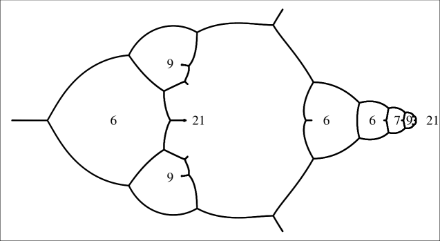
Figure 8.1. The dessin corresponding to $f_{96}(j,x)$. Besides the nine regions with indicated sizes there is a tenth region of size $1$ immediately to the left of the centrally printed $21$. This small region is adjacent to two triple points and near an endpoint. Also to the immediate right of each of the two left-printed nines, there is one triple point and two endpoints.

Figure 8.1 draws the dessin of $f_{96}(j,x)$, not in the copy of ${\mathbb{C}}$ with coordinate $x$, but rather the copy of ${\mathbb{C}}$ with coordinate $x^{\prime}=1/(1-x)$, for better geometric appearance. By definition, the figure consists of all $x^{\prime}$ corresponding to $x$ satisfying $f_{96}(j,x)=0$ with $j\in[0,1]$. This figure has the natural structure of a graph with $96$ edges, the preimages of $(0,1)$. All vertices have degree $\leq 3$: there are thirty-two triple points, the preimages of $0$, and forty double points and sixteen endpoints, the preimages of $1$. The forty double points are not readily visible in the figure, as they lie in the middle of forty double edges, but most of the triple points and endpoints are. There are also ten regions, of varying size, defined as half the number of bounding edges. The few aspects of all this structure which are not visible are described in the caption of Figure 8.1. The topological structure could also be deduced from a braid computation, rather than from the defining equation.

The polynomial $f_{96}(j,x)$ and Figure 8.1 illustrate the nature and complexity of the objects we are considering. Note that the existence of this cover shows that the Hurwitz number algebra indexed by $(A_{96},\;(3^{32},\,2^{40}\,1^{16},\,21^{2}\,9^{3}\,7\;6^{3}\,2),\;(1,1,1))$ has at least one factor of ${\mathbb{Q}}$. The entire Hurwitz algebra is way out of computational range, because the two main terms in the mass formula (3.6) give $3\times 10^{15}$ as an approximation for its degree.

A common feature of $f_{25}(j,x)$ from §4.2 and $f_{96}(j,x)$ is not accidental. In the braid group description of their monodromy, calculable purely group-theoretically, local monodromy operators about $0$ and $1$ are the images of braid group elements of order $3$ and $2$ respectively. Thus the preimage of $u=1/3$ in ${\sf X}_{h}\rightarrow{\sf U}_{4,1}$ for any $h$ with multiplicity vector $(4,1)$ likewise has this property.

8.3. Specialization and Newton polygons

For greater explicitness, we report only on specializing $f_{96}(j,x)$ to $j\in{\mbox{\sc U}}_{3,1}({\mathbb{Z}}[1/42])$. From complete tables of elliptic curves [6], this specialization set has size $413$. Supporting Principle A, all $413$ algebras are non-isomorphic. Supporting Principle B, these algebras all have Galois group $A_{96}$. Investigating Principle C is more subtle. In lieu of completely factoring $f_{96}(j,x)$ over ${\mathbb{Q}}_{p}$ and taking field discriminants of the factors, we use Newton polygons. To illustrate this computationally much simpler method, we take $j=1/3$ as a representative example, and work with

$$g(x)=3f(1/3,x)=3^{7}7^{21}x^{96}-2^{7}3^{7}7^{21}x^{95}+\cdots+2^{53}3^{32}x-2^{48}3^{31}.$$

Factoring modulo $2$, $3$, and $7$ gives

$$g(x) \stackrel{{\scriptstyle 2}}{{\equiv}}x^{96}, g(x) \stackrel{{\scriptstyle 3}}{{\equiv}}x^{54}(x-2)^{33}, g(x) \stackrel{{\scriptstyle 7}}{{\equiv}}h_{2}(x)h_{20}(x)h_{25}(x),$$

with $h_{k}(x)$ irreducible of degree $k$. The $2$-adic Newton polygon of $g(x)$ has all slopes $1/2$, showing that all $96$ roots $\alpha\in\overline{{\mathbb{Q}}}_{2}$ have ${\rm ord}_{2}(\alpha)=1/2$. Since the denominator is divisible by $2$, one has that the $2$-adic wild degree as in §4.5 is $m_{\rm 2\mbox{-}wild}=96$. From a more complicated calculation with $3$-adic Newton polygons, we get that the $96$ roots $\alpha\in\overline{{\mathbb{Q}}}_{3}$ are distributed as follows:

$$\begin{array}[]{rrclrrcl}\mbox{9 roots with}&{\rm ord}_{3}(\alpha)&=&4/9,&\;\;\;\mbox{22 roots with}&{\rm ord}_{3}(\alpha-1)&=&13/21,\\ \mbox{27 roots with}&{\rm ord}_{3}(\alpha)&=&1/3,&\mbox{3 roots with}&{\rm ord}_{3}(3\alpha-(1-i))&=&2/3,\\ \mbox{3 roots with}&{\rm ord}_{3}(\alpha)&=&-1/3,&\mbox{3 roots with}&{\rm ord}_{3}(3\alpha-(1+i))&=&2/3,\\ \mbox{9 roots with}&{\rm ord}_{3}(\alpha/3-i)&=&5/9,&\\ \mbox{9 roots with}&{\rm ord}_{3}(\alpha/3+i)&=&5/9,&\mbox{12 roots with}&{\rm ord}_{3}(\alpha-1)&=&1/2.\\ \end{array}$$

Only the last twelve $\alpha$ could possibly not contribute to the $3$-adic wild degree, giving already $m_{\rm 3\mbox{-}wild}\geq 84$. But in fact these $\alpha$ satisfy ${\rm ord}_{3}(\alpha^{2}/3-2)=5/12$ so one has $m_{\rm 3\mbox{-}wild}=96$. Finally, the $7$-adic Newton polygon of $g(x)$ has slopes $0$ and $-3/7$ with multiplicities $47$ and $49$ respectively. The slope of $0$ corresponds to the isolated roots modulo $7$ and the slope of $-3/7$ then gives $m_{\rm 7\mbox{-}wild}=49$.

The Newton polygon process can be easily automated. It says that all $413$ algebras are wildly ramified at both $2$ and $3$. It says also that all algebras are wildly ramified at $7$ except for those coming from the specialization points $-3^{1}5^{3}7^{3}/2^{8}$, $-7^{3}/2^{1}3^{2}$, $7^{3}/2^{9}$, $7^{3}/3^{5}$, $7^{3}/2^{1}3^{3}$, $5^{3}7^{3}/3^{5}$, $2^{2}7^{3}/3$ and $7^{4}/2^{6}3$, $-7^{4}/2^{7}3^{4}$, $7^{4}$, $-7^{5}/2^{1}3^{8}$. The first seven all have tame ramification at $7$ corresponding to the partition $19^{3}1^{39}$ while the last four have tame ramification at $7$ corresponding to the partition $57^{1}3^{13}$. This behavior comes from the fact that these specialization points are all $7$-adically close to $j=0$ and the degree $32$ polynomial above has tame ramification at $7$ given by the partition $19^{1}1^{13}$.

9. A degree 202 family: degenerations and generic specialization

Continuing to increase degrees as we go through the last six sections, we now describe a family having degree $202$. Our description emphasizes its degenerations, a relevant topic because how a family degenerates has substantial influence on how ramification behaves in the Hurwitz number fields within the family. We conclude by observing that specialization is generic, both in one of the degenerations of the family and in the family itself.

9.1. Some plane curves

To streamline the subsequent subsections, we first present some polynomials defining affine curves in the $x$-$y$ plane. The next two subsections will place a natural function on each curve, and we index the polynomials by the degree of this function.

Eleven relatively simple polynomials are

$$A_{10} =x, B_{4} =x-1,$$

$$A_{13} =y, B_{8} =y-1,$$

$$A_{14} =x-y, B_{32} =x^{2}y-4x^{2}-8xy+20x+10y-20,$$

$$A_{16} =3xy-6x-6y+10, C_{22} =3xy^{2}-12xy+8x-15y^{2}+40y-24,$$

$$A_{20} =x^{2}y-3x^{2}-6xy C_{25} =3x^{2}y-6x^{2}-12xy+20x+10y-15,$$

$$\qquad+12x+6y-10, D_{10} =3x^{2}-12x+10.$$

For all but one of these polynomials $P$, the curve ${\sf P}$ given by its vanishing is obviously rational, as at least one of the variables appears to degree one in $P$. In contrast, the curve ${\mbox{\sf D}}_{10}$ consists of two genus zero components, neither one of which is defined over ${\mathbb{Q}}$.

$${\begin{array}[]{r|rrrrr}B_{52}&1&x&x^{2}&x^{3}&x^{4}\\ \hline\cr 1&1080&-2160&1296&-176&-24\\ y&-1080&2052&-1164&156&12\\ y^{2}&135&-276&180&-36&\\ y^{3}&50&-84&36&&\\ y^{4}&15&-12&&&\\ \end{array}\;\;\;\;\;\;\;\;\;\begin{array}[]{r|rrrrr}D_{32}&1&x&x^{2}&x^{3}&x^{4}\\ \hline\cr 1&&&160&-192&48\\ y&&-320&192&120&-48\\ y^{2}&250&12&-213&12&12\\ y^{3}&-300&288&-18&-12&\\ y^{4}&90&-108&27&&\\ \end{array}}$$

 

$$\begin{array}[]{r|rrrrrrr}D_{48}&1&x&x^{2}&x^{3}&x^{4}&x^{5}&x^{6}\\ \hline\cr 1&&&&1600&-2880&1632&-288\\ y&&&2400&-8160&9048&-3960&576\\ y^{2}&&1200&-6480&11448&-8712&2880&-324\\ y^{3}&-2500&6300&-4620&-108&1395&-513&54\\ y^{4}&1500&-3900&3780&-1692&351&-27&\\ \end{array}$$

Table 9.1. Three polynomials $\sum c_{ij}x^{i}y^{j}$, presented by listing their coefficients $c_{ij}$.

Three more complicated polynomials are given in matrix form in Table 9.1. The corresponding curves ${\mbox{\sf B}}_{52}$, ${\mbox{\sf D}}_{32}$, and ${\mbox{\sf D}}_{48}$ have genus $1$, $2$, and $5$ respectively. Each genus is much smaller than the upper bound allowed by the support in ${\mathbb{Z}}_{\geq 0}^{2}$ of the coefficients; this bound, being the number of “interior” coefficients, is $6$, $6$, and $12$ respectively. In each case, there are several singularities causing this genus reduction, one of which is at $(1,1)$.

9.2. Calculation of a rational presentation.

This subsection is very similar to §6.1, illustrating that in favorable cases computation of Hurwitz covers following the outline of §3.7 is quite mechanical. As normalized Hurwitz parameter we take

$$h=(S_{6},(21111,3_{0}21,3_{1}111,4_{\infty}11),(2,1,1,1)).$$

Any function governed by $h$ is of the form

$$g(s)=\frac{s^{3}(s-x)^{2}(s-y)}{a\left(s^{2}+s(d-e-1)+e\right)}.$$

The ramification requirement on $g$ at $1$ is that $(g(1),g^{\prime}(1),g^{\prime\prime}(1))=(1,0,0)$. These three equations let us express $a$, $d$, and $e$ in terms of $x$ and $y$. Namely

$$a =-C_{25}, d =\frac{B^{2}_{4}B_{8}}{C_{25}}, e =\frac{A_{20}}{C_{25}}.$$

Using a resolvent as usual, we find that the critical values of $g(s)$ besides $0$, $1$, and $\infty$ are the roots of $Wt^{2}+(V-U-W)t+Ut^{2}$ with

(9.1) $$U = -2^{2}3^{3}A_{10}^{5}A_{13}^{4}A_{14}^{3}A_{16}A_{20}^{2},$$

(9.2) $$V = -3^{3}B_{4}B_{8}^{2}B_{32}^{4}B_{52},$$

(9.3) $$W = 2^{8}C_{25}^{5}C_{22}.$$

Comparing with the standard quadratic $t^{2}+(v-u-1)t+u$, one gets the rational presentation

(9.4) $$u =\frac{U}{W}, v =\frac{V}{W}.$$

So, appealing to (9.1)-(9.3) and the explicit polynomials in §9.1, Equations (9.4) express $u$ and $v$ as explicit functions of $x$ and $y$.

9.3. A view of ${\sf X}_{h}$

Recall from §6.2 and Figure 6.1 that the complement of ${\sf U}_{2,1,1,1}$ in the projective $u$-$v$-plane consists of three lines A, B, ${\sf C}$ and a conic D. In the map from the affine $x$-$y$ plane to the projective $u$-$v$ plane, we can consider the preimages of these discriminantal curves.

Figure 9.1. ${\mbox{\sc X}}_{h}({\mathbb{R}})$ is the complement of the drawn curves in the real $x$-$y$ plane. The drawn points are the ten real preimages of $(u,v)=(1,1)$.

Figure 9.1 draws the real points of these four preimages. Using as before a similar notation for an equation and its curve, inspection of our equations gives

$$\pi_{h}^{-1}({\mbox{\sf A}}) = {\mbox{\sf A}}_{10}\cup{\mbox{\sf A}}_{14}\cup{\mbox{\sf A}}_{13}\cup{\mbox{\sf A}}_{16}\cup{\mbox{\sf A}}_{20},$$

$$\pi_{h}^{-1}({\mbox{\sf B}}) = {\mbox{\sf B}}_{4}\cup{\mbox{\sf B}}_{8}\cup{\mbox{\sf B}}_{32}\cup{\mbox{\sf B}}_{52},$$

$$\pi_{h}^{-1}({\sf C}) = {\sf C}_{25}\cup{\sf C}_{22},$$

$$\pi_{h}^{-1}({\mbox{\sf D}}) = {\mbox{\sf D}}_{10}\cup{\mbox{\sf D}}_{32}\cup{\mbox{\sf D}}_{48}.$$

The figure is intended to indicate the rich geometry present in any Hurwitz surface. Other interesting curves present whenever $\nu=(2,1,1,1)$ are the preimages of the lines ${\sf ad}$, ${\sf bd}$, ${\sf cd}$, ${\sf bc}$, ${\sf ac}$, and ${\sf ab}$ introduced in §6. For the current $h$, all of them have a complicated real locus. Their genera are respectively $25$, $18$, $23$, $35$, $31$, and $23$. The curves ${\sf ad}$, ${\sf bd}$, and ${\sf cd}$ intersect at the preimage of the point ${\sf d}$, and Figure 9.1 also draws the ten real points of this preimage.

9.4. Degree $202$ polynomials and their degenerate factorizations

Removing $y$ and $x$ respectively from (9.4) by resultants gives degree $202$ polynomials $f(u,v,x)$ and $\phi(u,v,y)$. Completely expanded, they have 10484 and 15555 terms respectively.

The structures studied in the previous two subsections appear when one factors specializations corresponding to the four discriminantal components:

$$f(0,v,x) = x^{50}(x^{2}-4x+6)a_{13}(v,x)^{4}a_{14}(v,x)^{3}a_{16}(v,x)a_{20}(v,x)^{2},$$

$$f(u,0,x) = -(x-1)^{6}b_{8}(u,x)^{2}b_{32}(u,x)^{4}b_{52}(u,x),$$

$$\lim_{u\rightarrow\infty}\frac{f(u,wu,x)}{u^{10}} = -2^{10}(x-1)^{7}c_{10}(w,x)^{3}c_{22}(w,x)c_{25}(w,x)^{5},$$

$$f(r^{2},(1-r)^{2},x) = -(3x^{2}-12x+10)^{5}d_{32}(r,x)^{3}d_{48}(r,x)^{2},$$

and

$$\phi(0,v,y) = y^{52}(3y^{2}-8y+8)\alpha_{10}(v,y)^{5}\alpha_{14}(v,y)^{3}\alpha_{16}(v,y)\alpha_{20}(v,y)^{2},$$

$$\phi(u,0,y) = (y-1)^{16}(y-4)^{2}\beta_{4}(u,y)\beta_{32}(u,y)^{4}\beta_{52}(u,y),$$

$$\lim_{u\rightarrow\infty}\frac{\phi(u,wu,y)}{u^{13}} = -2^{36}(y-2)^{3}(y-1)^{7}\gamma_{6}(w,y)^{2}\gamma_{22}(w,y)\gamma_{25}(w,y)^{5},$$

$$\phi(r^{2},(1-r)^{2},y) = \delta_{10}(r,y)\delta_{32}(r,y)^{3}\delta_{48}(r,y)^{2}.$$

Our notation coordinates the different viewpoints: for example, the equations $D_{48}=0$, $d_{48}(r,x)=0$, and $\delta_{48}(r,y)=0$ all describe the genus five curve ${{\mbox{\sf D}}}_{48}$.

As a sample degeneration, chosen because it makes an interesting comparison the degree $25$ polynomials from our introductory example,

$$c_{25}(w,x)=$$

$$-(2x-5)(3x-5)^{2}\left(6x^{4}-40x^{3}+105x^{2}-120x+50\right)^{4}$$

$$\qquad\left(12x^{6}-60x^{5}-40x^{4}+760x^{3}-1800x^{2}+1750x-625\right)$$

$$+4wx^{5}(x^{2}-5x+5)^{3}(3x^{2}-10x+10)^{2}(6x^{2}-20x+15)^{4}(6x^{2}-15x+10).$$

Here the $x$-line is identified with ${\sf X}_{h}$ for $h=(S_{6},(321,3111,51,21111),(1,1,1,1))$, and the the $w$-line with ${\sf U}_{1,1,1,1}$. All the other degenerations have a similar four-point description. The discriminant of $c_{25}(w,x)$ is $2^{212}3^{66}5^{285}w^{13}(w-1)^{19}$. All the other degenerations are likewise three-point covers, all full except for ${\mbox{\sf A}}_{14}$, ${\mbox{\sf A}}_{16}$, ${\mbox{\sf A}}_{20}$, ${\sf C}_{6}$, and ${\mbox{\sf D}}_{10}$. In every case, the target variable, be it $v$, $u$, $w$, or $r$, is chosen such that the singular values are $0$, $1$, and $\infty$.

To be noted is that we are not expending any extra effort here to introduce a conceptually defined completion of ${\sf X}_{h}$. Indeed the curves that consist of horizontal lines, namely ${\mbox{\sf A}}_{13}$ and ${\mbox{\sf B}}_{8}$, are seen clearly by $f$ but only as vestigial factors by $\phi$. In reverse, the curves that consist of vertical lines, namely ${\mbox{\sf A}}_{10}$, ${\mbox{\sf B}}_{4}$, and ${\mbox{\sf D}}_{10}$, are seen completely by $\phi$ but only partially by $f$. Finally, to see preimages corresponding to the factors $c_{10}(w,x)$ and $\gamma_{6}(w,x)$, one would have to go beyond the $x$-$y$ plane as a partial completion of ${\sf X}_{h}$.

A braid group computation gives the partition of 202 which captures how local sheets of ${\sf X}_{h}$ are interchanged as one goes around one of the four discriminantal components in the completion of ${\sf U}_{2,1,1,1}$. These partitions are

$$\beta_{A} =5^{10}4^{13}3^{14}2^{20}1^{16+\mathbf{2}}, \beta_{B} =4^{32}2^{8+\mathbf{1}}1^{52+4}, \beta_{C} =5^{25}3^{10+\mathbf{2}}2^{6+\mathbf{2}}1^{22+\mathbf{3}},$$

and $\beta_{D}=3^{32}2^{48}1^{10}$. The boldface exponents correspond to components not seen by our simple calculations. Thus we are missing only $2$, $2$, $13$, and $0$ of the $202$ sheets near the preimages of A, B, ${\sf C}$, and D respectively.

9.5. Specialization

The degenerations can be specialized, and the computations support Principles A, B, and C. For example, consider $c_{25}(w,x)$ specialized to $w$ in the known set ${\mbox{\sc U}}_{1,1,1,1}({\mathbb{Z}}[1/30])$. The $99$ algebras are all distinct, they are all full, and they are all wildly ramified at each of $2$, $3$, and $5$. The wild ramification is even less than in our introductory example described in and around Figure 4.2 for two reasons. First, the algebras decompose more here; in particular, there are no $2$-adic factors of degree $16$ and no $5$-adic factors of degree $25$. Second, the individual factors are less ramified; for example, $2$-adic octics have a largest discriminant of $2^{26}$ rather than $2^{31}$ and $3$-adic nonics have a largest discriminant of $3^{16}$ rather than $3^{26}$. The mean exponents are now $(\langle a\rangle,\langle b\rangle,\langle c\rangle)\approx(47,32,35)$ rather than $(56,43,42)$; the maximum exponents are now $(a_{\rm max},b_{\rm max},c_{\rm max})=(61,38,44)$ rather than $(79,57,52)$.

Specialization of the full family at the $2947$ points of ${\mbox{\sc U}}_{2,1,1,1}({\mathbb{Z}}[1/30])$ can also be satisfactorily studied, despite the large degree. The $2947$ algebras are all distinct and they all have Galois group $A_{202}$ or $S_{202}$. From Newton polygons, we know they are all wildly ramified at $2$, $3$, and $5$. Thus, in this family, Principles A, B, and C hold without exception.

10. A degree 1200 field: computations in large degree

Conjecture 1.1 says that for certain finite sets of primes $\mathcal{P}$, there exist full number fields of arbitrarily large degree with ramification set in $\mathcal{P}$. A natural computational challenge for a given $\mathcal{P}$ is then to produce an explicit full Hurwitz number field $K_{h,u}$ with degree $m$ as large as possible. In this short final section, we take $\mathcal{P}=\{2,3,5\}$ and produce such a field for degree $m=1200$.

Taking $h=(S_{6},(21111,3_{0}2_{1}1,4_{\infty}11),(4,1,1))$ and normalizing as indicated, the functions to consider are

$$g(s)=\frac{as^{3}(s-1)^{2}(s-x)}{s^{2}+bs+c}.$$

As specialization point, we take $u=((t^{4}-4t-6),\{0\},\{\infty\})$. This specialization point indeed keeps ramification within $\{2,3,5\}$ as the discriminant of $t^{4}-4t-6$ is $-2^{8}3^{5}$.

The condition that the critical values besides $0$ and $\infty$ are the roots of $t^{4}-4t-6$ gives four equations in the four unknowns $x$, $a$, $b$, $c$. Of the unknowns, we are focusing on $x$ because its special values $0$, $1$, and $\infty$ are all meaningful, corresponding to degenerations. Eliminating $a$ and then $c$ is easy. Eliminating $b$ then has a ten-minute run-time on Magma to get a degree 3700 polynomial. Factorizing this polynomial to find the relevant factor has a one-minute run-time. The resulting monic polynomial $f_{1200}(x)\in{\mathbb{Z}}[1/30][x]$ defining $K_{h,u}$ satisfies $f_{1200}(0)=2^{880}/5^{500}$ and $f_{1200}(1)=3^{684}/2^{256}5^{500}$. After removing all factors of $2$, $3$, and $5$, the coefficients are integers averaging about $440$ digits.

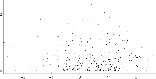
Figure 10.1. Roots in the closed upper half plane of a polynomial defining a degree $1200$ Hurwitz number field

The polynomial is to some extent analyzable despite its large degree and large coefficients. From the factorization partitions $(989,208,3)$ at $19$ and $(1181,9,6,4)$ at $47$, it has Galois group $S_{1200}$, in conformity with Principle B. From Newton polygons, it is wildly ramified at $2$, $3$, and $5$, as predicted by Principle C. Figure 10.1 presents the roots of $f_{1200}(x)$ in the closed upper half plane, all of which lie in the drawn window $[-2.6,2.6]\times[0,2.4]$. There are $34$ real roots and a general tendency of roots to cluster near the interval $[0,1]$ connecting the special points $0$ and $1$.

Large degree Hurwitz number fields provide specific challenges to improve computational algorithms for general number fields. For example, from Newton polygons we have substantial information on how the field $K_{h,u}$ of this section factors over ${\mathbb{Q}}_{2}$, ${\mathbb{Q}}_{3}$, and ${\mathbb{Q}}_{5}$. However we cannot go far enough to determine the exponents in its discriminant $-2^{a}3^{b}5^{c}$.

References

- [1] José Bertin and Matthieu Romagny, Champs de Hurwitz, Mém. Soc. Math. Fr. (N.S.) (2011), no. 125-126, 219. MR 2920693
- [2] Manjul Bhargava, The density of discriminants of quartic rings and fields, Ann. of Math. (2) 162 (2005), no. 2, 1031–1063. MR 2183288
- [3] by same author, Mass formulae for extensions of local fields, and conjectures on the density of number field discriminants, Int. Math. Res. Not. IMRN (2007), no. 17, Art. ID rnm052, 20. MR 2354798
- [4] by same author, The density of discriminants of quintic rings and fields., Ann. of Math. (2) 172 (2010), no. 3, 1559–1591.
- [5] Wieb Bosma, John Cannon, and Catherine Playoust, The Magma algebra system. I. The user language, J. Symbolic Comput. 24 (1997), no. 3-4, 235–265, Computational algebra and number theory (London, 1993). MR MR1484478
- [6] J. E. Cremona and M. P. Lingham, Finding all elliptic curves with good reduction outside a given set of primes, Experiment. Math. 16 (2007), no. 3, 303–312. MR 2367320
- [7] H. Davenport and H. Heilbronn, On the density of discriminants of cubic fields. II, Proc. Roy. Soc. London Ser. A 322 (1971), no. 1551, 405–420. MR 0491593
- [8] Claus Fieker and Jürgen Klüners, Computation of Galois groups of rational polynomials, LMS J. Comput. Math. 17 (2014), no. 1, 141–158. MR 3230862
- [9] John W. Jones and David P. Roberts, A database of number fields, LMS J. Comput. Math. 17 (2014), no. 1, 595–618, Database at http://hobbes.la.asu.edu/NFDB/. MR 3356048
- [10] Nicholas M. Katz, Rigid Local Systems, Annals of Mathematics Studies, vol. 139, Princeton University Press, Princeton, NJ, 1996. MR 1366651
- [11] Joachim Koenig, Computation of Hurwitz spaces and new explicit polynomials for almost simple Galois groups, Preprint, to appear in Math. Comp. 2015.
- [12] Gunter Malle, Multi-parameter polynomials with given Galois group, J. Symbolic Comput. 30 (2000), no. 6, 717–731. MR 1800034
- [13] Gunter Malle and B. Heinrich Matzat, Inverse Galois theory, Springer Monographs in Mathematics, Springer-Verlag, Berlin, 1999. MR 1711577
- [14] Gunter Malle and David P. Roberts, Number fields with discriminant and Galois group or , LMS J. Comput. Math. 8 (2005), 80–101 (electronic). MR 2135031
- [15] David P. Roberts, Hurwitz-Belyi maps, Arxiv, August 30, 2016. Submitted.
- [16] by same author, Wild partitions and number theory, J. Integer Seq. 10 (2007), no. 6, Article 07.6.6, 34. MR 2335791
- [17] by same author, Division polynomials with Galois group , Advances in the theory of numbers, Fields Inst. Commun., vol. 77, Fields Inst. Res. Math. Sci., Toronto, ON, 2015, pp. 169–206. MR 3409329
- [18] by same author, Polynomials with prescribed bad primes, Int. J. Number Theory 11 (2015), no. 4, 1115–1148. MR 3340686
- [19] David P. Roberts and Akshay Venkatesh, Hurwitz monodromy and full number fields, Algebra Number Theory 9 (2015), no. 3, 511–545. MR 3340543
- [20] Jean-Pierre Serre, Topics in Galois theory, second ed., Research Notes in Mathematics, vol. 1, A K Peters, Ltd., Wellesley, MA, 2008, With notes by Henri Darmon. MR 2363329
- [21] The PARI Group, Bordeaux, PARI/GP version 2.7.5, 2015, available from http://pari.math.u-bordeaux.fr/.
- [22] Helmut Völklein, A transformation principle for covers of , J. Reine Angew. Math. 534 (2001), 156–168. MR 1831635
- [23] Wolfram Research, Inc., Mathematica 10.0.2.0.