Singular Knots and Involutive Quandles

Abstract.

The aim of this paper is to define certain algebraic structures coming from generalized Reidemeister moves of singular knot theory. We give examples, show that the set of colorings by these algebraic structures is an invariant of singular links. As an application we distinguish several singular knots and links.

1. Introduction

The study of singular knots and their invariants was motivated mainly by the theory of Vassiliev invariants [Vassiliev]. Most of the important knot invariants have been extended to singular knot invariants. Fiedler extended the Kauffman state models of the Jones and Alexander polynomials to the context of singular knots [Fiedler]. Juyumaya and Lambropoulou constructed a Jones-type invariant for singular links using a Markov trace on a variation of the Hecke algebra [JL]. In [KV] Kauffman and Vogel defined a polynomial invariant of embedded $4$-valent graphs in $\mathbb{R}^{3}$ extending an invariant for links in $\mathbb{R}^{3}$ called the Kauffman polynomial [kaufgraph]. In [HN], Henrich and the fourth author investigated singular knots in the context of virtual knot theory, flat virtual knot theory and flat singular virtual knot theory. They introduced algebraic structures called semiquandles, singular semiquandles and virtual singular semiquandles. They also gave an application to distinguishing Vassiliev-type invariants of virtual knots. Other extensions of classical invariants of knots to singular knots can be found in the works of [St, Paris]. In this article we consider colorings of singular knots and links by certain algebraic structures. As in the case of classical knot theory [Prz] we show that the set of colorings is independent of the choice of the diagrams of a given singular knot or link making it an invariant of singular knots. We show that this invariant is computable. We then use it to distinguish many singular knots.

This article is organized as follows. In section 3, we review the basics of quandles and give examples. Section 4 gives the definition of singquandles with examples and shows that the set of colorings of singular links by a singquandle is an invariant of singular links. In section LABEL:sec4 we compute the coloring invariants for many singular links and use it to distinguish many singular links. In section 5 we collect some open questions for future research.

2. Acknowledgements

The fourth listed author was partially supported by Simons Foundation Collaboration Grant 316709.

3. Review of Quandles

We review the basics of quandle theory needed for this article. Quandles are non-associative algebraic structures that correspond to the axiomatization of the three Reidemeister moves in knot theory. Since the early eighties when quandles were introduced by Joyce [Joyce] and Matveev [Matveev] independently, there has been a lot of interest in the theory, (see for example the book [EN] and the references therein). Joyce and Matveev proved that the fundamental quandle of a knot is a complete invariant up to orientation. Precisely, given two knots $K_{0}$ and $K_{1}$, the fundamental quandle $Q(K_{0})$ is isomorphic to the fundamental quandle $Q(K_{1})$ if and only if $K_{1}$ is equivalent to $K_{0}$ or $K_{1}$ is equivalent to the reverse of the mirror image of $K_{0}$. Quandles have been used by topologists to construct invariants of knots in $3$-space and knotted surfaces in $4$-space. For example in [HN], Henrich and the fourth author investigated singular knots in the context of virtual knot theory. Their derived algebraic structure is called virtual semiquandle and it comes from some generalizations of Reidemeister moves for virtual knots. They used it to construct invariants to distinguish generalized knots, with an application to distinguishing Vassiliev-type invariants of virtual knots. Now we recall the basic definitions of quandles and give a few examples.

Definition 3.1.

A rack is a set $X$ with a binary operation $*$ satisfying the following two axioms:

• for all $x\in X$, the right multiplication $y\mapsto y*x$ by $x$ is a bijection, and

• $(x*y)*z=(x*z)*(y*z)$.

A rack which further satisfies $x*x=x$ for all $x\in X$ is called a quandle.

A quandle homomorphism between two quandles $X,Y$ is a map $f:X\rightarrow Y$ such that $f(x*y)=f(x)*f(y)$. A quandle isomorphism is a bijective quandle homomorphism, and two quandles are isomorphic if there is a quandle isomorphism between them. The right multiplication $R_{x}$ is the automorphism of $X$ given by $R_{x}(y)=y*x$. Its inverse will be denoted by $R_{x}^{-1}(y):=y*^{-1}x$. The set of all quandle isomorphisms of $X$ is a group denoted $Aut(X)$. Its subgroup generated by all right multiplications $R_{x}$ is called the Inner group and denoted $Inn(X)$. A quandle is called involutive if $(x*y)*y=x$ for all $x,y\in X$. In other words $R_{x}=R_{x}^{-1},\;\forall x\in X$.

Typical examples of quandles include the following.

• Any non-empty set $X$ with the operation $x*y=x$ for all $x,y\in X$ is a quandle called the trivial quandle.

• A group $X=G$ with $n$-fold conjugation as the quandle operation: $a*b=b^{-n}ab^{n}$.

• A group $X=G$ with the binary operation: $a*b=ba^{-1}b$ is a quandle. It is called the core quandle of the group $G$.

• Let $n$ be a positive integer. For $a,b\in\mathbb{Z}_{n}$ (integers modulo $n$), define $a*b\equiv 2b-a\pmod{n}$. Then $*$ defines a quandle structure called the dihedral quandle, $R_{n}$. This set can be identified with the set of reflections of a regular $n$-gon with conjugation as the quandle operation.

• Any ${\mathbb{Z}}[T,T^{-1}]$-module $M$ is a quandle with $a*b=Ta+(1-T)b$, $a,b\in M$, called an Alexander quandle.

In standard knot theory, to distinguish knots using quandles, one only needs to consider connected quandles according to section 5.2 in [Ohtsuki] (see also lemma 3.1 in [CESY]). A quandle is connected if for every $x,y\in X$, there exists a sequence of elements $x_{1},\ldots,x_{n}\in X$ for some positive integer $n$ and $\epsilon_{1},\epsilon_{2},\cdots\epsilon_{n}\in\{-1,1\}$ such that $(\cdots(x*^{\epsilon_{1}}x_{1})*^{\epsilon_{2}}x_{2})*^{\epsilon_{3}}\cdots)\cdots*^{\epsilon_{n}}x_{n})=y$. In other words the Inner group $Inn(X)$ acts transitively on the quandle $X$.

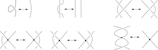
Figure 1. Classical Reidemeister moves $RI$, $RII$ and $RIII$ on the top and singular Reidemeister $RIVa$, $RIVb$ and $RV$ on the bottom.

4. Singular Quandles

In this section we define the notion of singquandles, give some examples and use them to construct an invariant of singular knots and links. The invariant is the set of colorings of a given singular knot or link by a singquandle. The colorings of regular and singular crossings are given by the following figure 2.

Figure 2. Regular and singular crossings

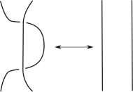
Figure 3. Reidemeister move II for regular crossings

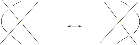
Figure 4. Reidemeister move III for regular crossings

Figure 5. The singular Reidemeister move RIVa and colorings

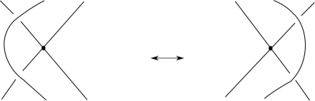
Figure 6. The singular Reidemeister move RIVb and colorings

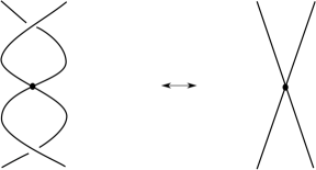
Figure 7. The singular Reidemeister move RV and colorings

Since our singular crossings are unoriented, we need the operations to be symmetric in the sense that if we rotate the crossing in the right diagram of figure 2 by $90$, $180$ or $270$ degrees, the operations should stay the same in order for colorings to be well-defined. Therefore we get the following three axioms:

(4.1) $$x = R_{1}(y,R_{2}(x,y))=R_{2}(R_{2}(x,y),R_{1}(x,y)),$$

(4.2) $$y = R_{2}(R_{1}(x,y),x)=R_{1}(R_{2}(x,y),R_{1}(x,y)),$$

(4.3) $$(R1(x,y),R2(x,y)) = (R_{2}(y,R_{2}(x,y)),R_{1}(R_{1}(x,y),x)).$$

The axioms of the following definition come from the generalized Reidemeister moves RIV and RV in the respective figures 6 and 7.

Definition 4.1.

Let $(X,*)$ be an involutive quandle. Let $R_{1}$ and $R_{2}$ be two maps from $X\times X$ to $X$. The triple $(X,*,R_{1},R_{2})$ is called a singquandle if, in addition to the three axioms 4.1,  4.2 and 4.3, the following axioms are satisfied

(4.4) $$(y*z)*R_{2}(x,z) = (y*x)*R_{1}(x,z)\;\;\;\text{coming from RIVa}$$

(4.5) $$R_{1}(x,y) = R_{2}(y*x,x)\;\;\;\text{coming from RV}$$

(4.6) $$R_{2}(x,y) = R_{1}(y*x,x)*R_{2}(y*x,x)\;\;\;\text{coming from RV}$$

(4.7) $$R_{1}(x*y,z)*y = R_{1}(x,z*y)\;\;\;\text{coming from RIVb}$$

(4.8) $$R_{2}(x*y,z) = R_{2}(x,z*y)*y\;\;\;\text{coming from RIVb}$$

As in the case of classical knot theory [Prz], the following straightforward lemma makes the set of colorings of a singular knot by singquandles an invariant of singular knots.

Lemma 4.2.

The set of colorings of a singular knot by a singquandle does not change by the moves RI, RII, RIII, $RIVa$, $RIVb$ and RV.

We end this section with a class of singquandles generalizing the class of involutive Alexander quandles.

Proposition 4.3.

Let $\Lambda=\mathbb{Z}[t,B]/(t^{2}-1,B(1+t),t-(1-B)^{2})$ and let $X$ be a $\Lambda$-module. Then the operations

$$x\ast y=tx+(1-t)y,\quad R_{1}(x,y)=(1-t-B)x+(t+B)y\quad\mathrm{and}\quad R_{2}(x,y)=(1-B)x+By$$

make $X$ an involutive singquandle we call an Alexander singquandle.

Proof.

It is straightforward to verify that $\ast$ makes $X$ an involutive quandle. We note that since $t^{2}=1$, we have

$$t(1-t)=t-t^{2}=t-1\quad\mathrm{and}\quad(1-t)^{2}=1-2t+t^{2}=2(1-t),$$

since $B(1+t)=0$, we have $Bt=-B$ and since $t-(1-B)^{2}=0$ we have

$$1-t-2B+B^{2}=0\quad\mathrm{and}\quad t+2B-B^{2}=1.$$

We verify that our operations satisfy the remaining singquandle axioms. First, we compute

$$R_{1}(y,R_{2}(x,y)) = (1-t-B)y+(t+B)((1-B)x+By)$$

$$= (1-t-B)y+(t+B)(1-B)x+(t+B)By$$

$$= (1-t-B+tB+B^{2})y+(t+B)(1-B)x$$

$$= (1-t-B+tB+B^{2})y+(t+B-tB-B^{2})x$$

$$= (1-t-2B+B^{2})y+(t+2B-B^{2})x$$

$$= 0y+1x=x$$

and

$$R_{2}(R_{2}(x,y),R_{1}(x,y)) = (1-B)((1-B)x+By)+B((1-t-B)x+(t+B)y)$$

$$= ((1-B)^{2}+B(1-t-B))x+B(1-B+t+B)y$$

$$= (t+B-tB-B^{2})x+B(1+t)y$$

$$= (t+2B-B^{2})x+B(1+t)y$$

$$= 1x+0y=x$$

and (4.1) is satisfied.

Next, we have

$$R_{2}(R_{1}(x,y),x) = (1-B)((1-t-B)x+(t+B)y)+Bx$$

$$= ((1-B)(1-t-B)+B)x+(1-B)(t+B)y$$

$$= (1-t-B-B+tB+B^{2}+B)x+(t+B-tB-B^{2})y$$

$$= (1-t-2B+B^{2})x+(t+2b-B^{2})y$$

$$= 0x+1y=y$$

and

$$R_{1}(R_{2}(x,y),R_{1}(x,y)) = (1-t-B)((1-B)x+By)+(t+B)((1-t-B)x+(t+B)y)$$

$$= (1-t-B)(1-B+t+B)x+(B(1-t-B)+(t+B)^{2})y$$

$$= (1-t-B)(1+t)x+(B-tB-B^{2}+t^{2}+2tB+B^{2})y$$

$$= (1-t-B+t-t^{2}-tB)x+1y$$

$$= 0x+1y$$

and axiom (4.2) is satisfied.

Continuing, we have

$$(R_{2}(y,R_{2}(x,y)),R_{1}(R_{1}(x,y),x)) = ((1-B)y+B((1-B)x+By),$$

$$\quad\quad(1-t-B)((1-t-B)x+(t+B)y)+(t+B)x)$$

$$= ((1-B+B^{2})y+B(1-B)x,$$

$$\quad\quad((1-t-B)^{2}+t+B)x+(1-t-B)(t+B)y)$$

$$= ((t+B)y+(B-B^{2})x,$$

$$\quad\quad(1-t-B-t+t^{2}+tB-B+tB+B^{2}+t+B)x$$

$$\quad\quad+(t-t^{2}-tB+B-tB-B^{2})y)$$

$$= ((1-t-B)x+(t+B)y,(1-B)x+By)$$

$$= R(x,y)$$

as required by axiom (4.3).

Next, we have

$$(y\ast z)\ast R_{2}(x,z) = t(ty+(1-t)z)+(1-t)((1-B)x+Bz)$$

$$= (1-t)(1-B)x+t^{2}y+(1-t)(t+B)z$$

$$= (1-t)(t+1-t-B)x+t^{2}y+(1-t)(t+B)z$$

$$= t(ty+(1-t)x)+(1-t)((1-t-B)x+(t+B)z)$$

$$= (y\ast x)\ast R_{1}(x,z)$$

and we have (4.4). Next, we have

$$R_{1}(x,y) = (1-t-B)x+(t+B)y$$

$$= (1-t-B+tB+B)x+(t-tB)y$$

$$= ((1-B)(1-t)+B)x+(1-B)ty$$

$$= (1-B)(ty+(1-t)x)+Bx$$

$$= R_{2}(y\ast x,x)$$

and we have (4.5). Continuing, we have

$$R_{2}(x,y) = (1-B)x+By$$

$$= (1-B+(1-t-B)(t-1)+(1-t)(1-t-B))x+(1-t-B+t+B-1+B)y$$

$$= ((1-t-B)(t-1)+1-B+(1-t)(1-t-B))x+(1-t-B+t-tB-1+B)y$$

$$= ((1-t-B)(t-1)+t^{2}+tB+(1-t)(1-t-B+tB+B))x$$

$$\quad\quad+(1-t-B+(t-1)(1-B))y$$

$$= (t(1-t-B)(1-t)+t(t+B)+(1-t)((1-t)(1-B)+B))x+(t^{2}(1-t-B)$$

$$\quad\quad+t(1-t)(1-B))y$$

$$= t((1-t-B)(ty+(1-t)x)+(t+B)x)+(1-t)((1-B)(ty+(1-t)x)+Bx)$$

$$= R_{1}(y\ast x,x)\ast R_{2}(y\ast x,x)$$

and we have (4.6).

Next, we have

$$R_{1}(x\ast y,z)*y = t((1-t-B)(tx+(1-t)y)+(t+B)z)+(1-t)y$$

$$= t^{2}(1-t-B)x+t(t+B)z+(1-t)(t(1-t-B)+1)y$$

$$= t^{2}(1-t-B)x+t(t+B)z+(1-t)(t-t^{2}-tB+1)y$$

$$= t^{2}(1-t-B)x+t(t+B)z+(1-t)(t+B)y$$

$$= (1-t-B)x+(t+B)(tz+(1-t)y)$$

$$= R_{1}(x,z\ast y)$$

as required by (4.7).

Lastly, we have

$$R_{2}(x\ast y,z) = (1-B)(tx+(1-t)y)+Bz$$

$$= t(1-B)x+t^{2}Bz+(1-t)(1+tB)y$$

$$= t((1-B)x+B(tz+(1-t)y))+(1-t)y$$

$$= R_{2}(x,z\ast y)\ast y$$

as required. Hence, all axioms in Definition 4.1 are also satisfied. This completes the proof. ∎

Example 4.4.

Any abelian group $A$ becomes an involutive Alexander singquandle by choosing an involutive automorphism $t:A\to A$ and another homomorphism $B:A\to A$ satisfying the conditions $B(x)=-Bt(x)$ and $t(x)=(x-B(x))^{2}$ for all $x\in A$. More concretely, any commutative ring $R$ with identity becomes an involutive Alexander singquandle by choosing elements $t,B\in R$ such that $t^{2}=1$, $B(1+t)=0$ and $t-(1-B)^{2}=0$ and setting

$$x\ast y=tx+(1-t)y,\quad R_{1}(x,y)=(1-t-B)x+(t+B)y\quad\mathrm{and}\quad R_{2}(x,y)=(1-B)x+By.$$

For example, in $\mathbb{Z}_{5}$ with $t=4$ and $B=3$ we have $t^{2}=4^{2}=16=1$, $B(1+t)=3(1+4)=15=0$ and $t-(1-B)^{2}=4-(1-3)^{2}=4-4=0$, so $X=\mathbb{Z}_{5}$ is an involutive Alexander singquandle with

$$x\ast y=4x+2y,\quad R_{1}(x,y)=4x+2y\quad\mathrm{and}\quad R_{2}(x,y)=3x+3y.$$

5. Applications

Let $X$ be a $\Lambda$-module with the operations

$$\begin{array}[]{rcl}x\ast y&=&tx+(1-t)y\\ R_{1}(x,y)&=&(1-t-B)x+(t+B)y\quad\mathrm{and}\\ R_{2}(x,y)&=&(1-B)x+By\end{array}$$

where $\Lambda=\mathbb{Z}[t,B]/(t^{2}-1,B(1+t),t-(1-B)^{2})$.

Example 5.1.

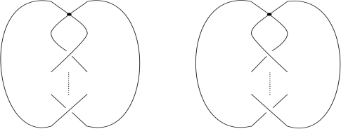
Figure 8. One singular crossing followed by $(n+1)$ regular crossings

We color the top two strands of the knot on the left side of Figure 8 and assume that the integer $n=2k$ is even.

For the knot on the left then the condition of colorability gives the following system of equations

$$x = (-k+kt)R_{1}(x,y)+(k+1-kt)R_{2}(x,y)$$

$$y = [-k+(k+1)t]R_{1}(x,y)+[k+1-(k+1)t]R_{2}(x,y).$$

This system of equations simplifies to

$$(1-B)^{2}(x-y) = 0$$

$$(-kt+B+k)(x-y) = 0.$$

thus forcing $x=y$ and consequently in this case the set of colorings is the diagonal inside $X\times X$.

For the knot on the right we also assume $n=2k$. Then the condition of colorability gives the following system of equations

$$x = (k-kt)R_{1}(x,y)+(1-k+kt)R_{2}(x,y)$$

$$y = [k+1-kt]R_{1}(x,y)+[-k+kt]R_{2}(x,y).$$

which simplifies to

$$(-k+kt+B)(x-y) = 0$$

$$(-1+k+t-k+B)(x-y) = 0.$$

implying that

$$-k+kt+B = 0$$

$$-1+k+t-k+B = 0.$$

Now by choosing $t=1$, one obtains the single equation $B(x-y)=0$. Since $B$ doesn’t have to be invertible, a right choice of a zero divisor value for $B$ will give that the coloring space contains the diagonal of $X\times X$ as a proper subset and thus the two links will be distinguished by the coloring sets.

Example 5.2.

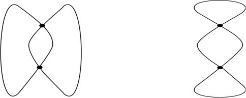
Figure 9. Two singular knots each with two singular crossings

Consider the knot on the left of Figure 9 and color the two top arcs by elements $x$ and $y$. By writing the relations at the crossings we get the two equations

$$x = R_{1}(R_{1}(x,y),R_{2}(x,y))\quad\mathrm{and}$$

$$y = R_{2}(R_{1}(x,y),R_{2}(x,y)).$$

We thus obtain after simplification $(t-1+2B)(y-x)=0$. Thus the set of all colorings of the knot on the left is

$$\{(x,y)\in X\times X\ |\ (t-1+2B)(y-x)=0\}.$$

It is clear that the knot on the right of Figure 9 colors trivially by the whole quandle. By choosing $\mathbb{Z}_{10}[t,B]$ with $t=-1$ and $B=4$, thus the coloring invariant distinguishes these two singular knots.

Example 5.3.

For our final example, we computed singquandle colorings for certain singular knots known as two-bouquet graphs using the singquandle structure on the set $X=\{1,2,3,4,5\}$ specified by the following operation tables where $R_{1}(x,y)=R_{2}(x,y)=x\ast^{\prime}y$:

$$\begin{array}[]{r|rrrrr}\ast&1&2&3&4&5\\ \hline\cr 1&1&3&5&2&4\\ 2&5&2&4&1&3\\ 3&4&1&3&5&2\\ 4&3&5&2&4&1\\ 5&2&4&1&3&5\end{array}\quad\begin{array}[]{r|rrrrl}\ast^{\prime}&1&2&3&4&5\\ \hline\cr 1&1&4&2&5&3\\ 2&4&2&5&3&1\\ 3&2&5&3&1&4\\ 4&5&3&1&4&2\\ 5&3&1&4&2&5.\end{array}$$

Then the singular knot on the left has five colorings by $X$ while the one on the right has 25:

References

- [1] BatainehKhaledElhamdadiMohamedHajijMustafaThe colored jones polynomial of singular knotsNew York J. Math.2220161439–1456ISSN 1076-9803Review MathReviews@article{BEH, author = {Bataineh, Khaled}, author = {Elhamdadi, Mohamed}, author = {Hajij, Mustafa}, title = {The colored Jones polynomial of singular knots}, journal = {New York J. Math.}, volume = {22}, date = {2016}, pages = {1439–1456}, issn = {1076-9803}, review = {\MR{3603072}}}
- [3] BirmanJoan S.New points of view in knot theoryBull. Amer. Math. Soc. (N.S.)2819932253–287ISSN 0273-0979Review MathReviewsDocument@article{Birman, author = {Birman, Joan S.}, title = {New points of view in knot theory}, journal = {Bull. Amer. Math. Soc. (N.S.)}, volume = {28}, date = {1993}, number = {2}, pages = {253–287}, issn = {0273-0979}, review = {\MR{1191478 (94b:57007)}}, doi = {10.1090/S0273-0979-1993-00389-6}}
- [5] BirmanJoan S.LinXiao-SongKnot polynomials and vassiliev’s invariantsInvent. Math.11119932225–270ISSN 0020-9910Review MathReviewsDocument@article{BL, author = {Birman, Joan S.}, author = {Lin, Xiao-Song}, title = {Knot polynomials and Vassiliev's invariants}, journal = {Invent. Math.}, volume = {111}, date = {1993}, number = {2}, pages = {225–270}, issn = {0020-9910}, review = {\MR{1198809}}, doi = {10.1007/BF01231287}} CarterJ. ScottElhamdadiMohamedSaitoMasahicoSilverDaniel S.WilliamsSusan G.Virtual knot invariants from group biquandles and their cocyclesJ. Knot Theory Ramifications1820097957–972ISSN 0218-2165Review MathReviewsDocument@article{CESSW, author = {Carter, J. Scott}, author = {Elhamdadi, Mohamed}, author = {Saito, Masahico}, author = {Silver, Daniel S.}, author = {Williams, Susan G.}, title = {Virtual knot invariants from group biquandles and their cocycles}, journal = {J. Knot Theory Ramifications}, volume = {18}, date = {2009}, number = {7}, pages = {957–972}, issn = {0218-2165}, review = {\MR{2549477}}, doi = {10.1142/S0218216509007269}}
- [8] ClarkW. EdwinElhamdadiMohamedSaitoMasahicoYeatmanTimothyQuandle colorings of knots and applicationsJ. Knot Theory Ramifications23201461450035, 29ISSN 0218-2165Review MathReviewsDocument@article{CESY, author = {Clark, W. Edwin}, author = {Elhamdadi, Mohamed}, author = {Saito, Masahico}, author = {Yeatman, Timothy}, title = {Quandle colorings of knots and applications}, journal = {J. Knot Theory Ramifications}, volume = {23}, date = {2014}, number = {6}, pages = {1450035, 29}, issn = {0218-2165}, review = {\MR{3253967}}, doi = {10.1142/S0218216514500357}}
- [10] ElhamdadiMohamedNelsonSamQuandles—an introduction to the algebra of knotsStudent Mathematical Library74American Mathematical Society, Providence, RI2015x+245ISBN 978-1-4704-2213-4Review MathReviews@book{EN, author = {Elhamdadi, Mohamed}, author = {Nelson, Sam}, title = {Quandles—an introduction to the algebra of knots}, series = {Student Mathematical Library}, volume = {74}, publisher = {American Mathematical Society, Providence, RI}, date = {2015}, pages = {x+245}, isbn = {978-1-4704-2213-4}, review = {\MR{3379534}}}
- [12] FiedlerThomasThe jones and alexander polynomials for singular linksJ. Knot Theory Ramifications1920107859–866ISSN 0218-2165Review MathReviewsDocument@article{Fiedler, author = {Fiedler, Thomas}, title = {The Jones and Alexander polynomials for singular links}, journal = {J. Knot Theory Ramifications}, volume = {19}, date = {2010}, number = {7}, pages = {859–866}, issn = {0218-2165}, review = {\MR{2673687 (2012b:57024)}}, doi = {10.1142/S0218216510008236}}
- [14] HenrichAllisonNelsonSamSemiquandles and flat virtual knotsPacific J. Math.24820101155–170ISSN 0030-8730Review MathReviewsDocument@article{HN, author = {Henrich, Allison}, author = {Nelson, Sam}, title = {Semiquandles and flat virtual knots}, journal = {Pacific J. Math.}, volume = {248}, date = {2010}, number = {1}, pages = {155–170}, issn = {0030-8730}, review = {\MR{2734169}}, doi = {10.2140/pjm.2010.248.155}}
- [16] JoyceDavidA classifying invariant of knots, the knot quandleJ. Pure Appl. Algebra231982137–65ISSN 0022-4049Review MathReviewsDocument@article{Joyce, author = {Joyce, David}, title = {A classifying invariant of knots, the knot quandle}, journal = {J. Pure Appl. Algebra}, volume = {23}, date = {1982}, number = {1}, pages = {37–65}, issn = {0022-4049}, review = {\MR{638121}}, doi = {10.1016/0022-4049(82)90077-9}}
- [18] JuyumayaJ.LambropoulouS.An invariant for singular knotsJ. Knot Theory Ramifications1820096825–840ISSN 0218-2165Review MathReviewsDocument@article{JL, author = {Juyumaya, J.}, author = {Lambropoulou, S.}, title = {An invariant for singular knots}, journal = {J. Knot Theory Ramifications}, volume = {18}, date = {2009}, number = {6}, pages = {825–840}, issn = {0218-2165}, review = {\MR{2542698 (2010i:57028)}}, doi = {10.1142/S0218216509007324}}
- [20] KauffmanLouis H.Invariants of graphs in three-spaceTrans. Amer. Math. Soc.31119892697–710ISSN 0002-9947Review MathReviewsDocument@article{kaufgraph, author = {Kauffman, Louis H.}, title = {Invariants of graphs in three-space}, journal = {Trans. Amer. Math. Soc.}, volume = {311}, date = {1989}, number = {2}, pages = {697–710}, issn = {0002-9947}, review = {\MR{946218}}, doi = {10.2307/2001147}}
- [22] KauffmanLouis H.VogelPierreLink polynomials and a graphical calculusJ. Knot Theory Ramifications11992159–104ISSN 0218-2165Review MathReviewsDocument@article{KV, author = {Kauffman, Louis H.}, author = {Vogel, Pierre}, title = {Link polynomials and a graphical calculus}, journal = {J. Knot Theory Ramifications}, volume = {1}, date = {1992}, number = {1}, pages = {59–104}, issn = {0218-2165}, review = {\MR{1155094}}, doi = {10.1142/S0218216592000069}}
- [24] MatveevS. V.Distributive groupoids in knot theoryRussianMat. Sb. (N.S.)119(161)1982178–88, 160ISSN 0368-8666Review MathReviews@article{Matveev, author = {Matveev, S. V.}, title = {Distributive groupoids in knot theory}, language = {Russian}, journal = {Mat. Sb. (N.S.)}, volume = {119(161)}, date = {1982}, number = {1}, pages = {78–88, 160}, issn = {0368-8666}, review = {\MR{672410}}}
- [26] OhtsukiT.Problems on invariants of knots and 3-manifoldsWith an introduction by J. Robertstitle={Invariants of knots and 3-manifolds}, address={Kyoto}, date={2001}, series={Geom. Topol. Monogr.}, volume={4}, publisher={Geom. Topol. Publ., Coventry}, 2002i–iv, 377–572Review MathReviewsDocument@article{Ohtsuki, author = {Ohtsuki, T.}, title = {Problems on invariants of knots and 3-manifolds}, note = {With an introduction by J. Roberts}, conference = {title={Invariants of knots and 3-manifolds}, address={Kyoto}, date={2001}, }, book = {series={Geom. Topol. Monogr.}, volume={4}, publisher={Geom. Topol. Publ., Coventry}, }, date = {2002}, pages = {i–iv, 377–572}, review = {\MR{2065029}}, doi = {10.2140/gtm.2002.4}}
- [28] ParisLuisThe proof of birman’s conjecture on singular braid monoidsGeom. Topol.820041281–1300 (electronic)ISSN 1465-3060Review MathReviewsDocument@article{Paris, author = {Paris, Luis}, title = {The proof of Birman's conjecture on singular braid monoids}, journal = {Geom. Topol.}, volume = {8}, date = {2004}, pages = {1281–1300 (electronic)}, issn = {1465-3060}, review = {\MR{2087084}}, doi = {10.2140/gt.2004.8.1281}}
- [30] PrzytyckiJózef H.-Coloring and other elementary invariants of knotstitle={Knot theory}, address={Warsaw}, date={1995}, series={Banach Center Publ.}, volume={42}, publisher={Polish Acad. Sci., Warsaw}, 1998275–295Review MathReviews@article{Prz, author = {Przytycki, J{\'o}zef H.}, title = {$3$-coloring and other elementary invariants of knots}, conference = {title={Knot theory}, address={Warsaw}, date={1995}, }, book = {series={Banach Center Publ.}, volume={42}, publisher={Polish Acad. Sci., Warsaw}, }, date = {1998}, pages = {275–295}, review = {\MR{1634462}}}
- [32] StoimenowA.On cabled knots and vassiliev invariants (not) contained in knot polynomialsCanad. J. Math.5920072418–448ISSN 0008-414XReview MathReviewsDocument@article{St, author = {Stoimenow, A.}, title = {On cabled knots and Vassiliev invariants (not) contained in knot polynomials}, journal = {Canad. J. Math.}, volume = {59}, date = {2007}, number = {2}, pages = {418–448}, issn = {0008-414X}, review = {\MR{2310624}}, doi = {10.4153/CJM-2007-018-0}}
- [34] VassilievV. A.Cohomology of knot spacestitle={Theory of singularities and its applications}, series={Adv. Soviet Math.}, volume={1}, publisher={Amer. Math. Soc., Providence, RI}, 199023–69Review MathReviews@article{Vassiliev, author = {Vassiliev, V. A.}, title = {Cohomology of knot spaces}, conference = {title={Theory of singularities and its applications}, }, book = {series={Adv. Soviet Math.}, volume={1}, publisher={Amer. Math. Soc., Providence, RI}, }, date = {1990}, pages = {23–69}, review = {\MR{1089670 (92a:57016)}}}
- [36] WadaMasaakiGroup invariants of linksTopology3119922399–406ISSN 0040-9383Review MathReviewsDocument@article{Wada, author = {Wada, Masaaki}, title = {Group invariants of links}, journal = {Topology}, volume = {31}, date = {1992}, number = {2}, pages = {399–406}, issn = {0040-9383}, review = {\MR{1167178}}, doi = {10.1016/0040-9383(92)90029-H}}
- [38]