Data processing for qubit state tomography:
An information geometric approach

Abstract

A statistically feasible data post-processing method for the conventional qubit state tomography is studied from an information geometrical point of view. It is shown that the space $(-1,1)^{3}$ of the Stokes parameters $({\xi}_{1},{\xi}_{2},{\xi}_{3})$ that specify qubit states should be regarded as a Riemannian manifold endowed with a metric $g_{ij}:={\delta}_{ij}/(1-({\xi}_{i})^{2})$, and that the data processing based on the maximum likelihood method is realized by the orthogonal projection from the empirical distribution onto the Bloch sphere with respect to the metric $g_{ij}$. An efficient algorithm for computing the maximum likelihood estimate is also proposed.

I Introduction

It is well known that there is a one-to-one affine correspondence between the quantum state space

$${\mathcal{S}}({\mathbb{C}}^{2}):=\{{\rho}\;|\;{\rho}\geq 0,\;{\rm Tr}\,{\rho}=1\}$$

on the two-dimensional Hilbert space ${\mathbb{C}}^{2}$ and the unit ball

$$B:=\left.\left\{{\xi}=({\xi}_{1},{\xi}_{2},{\xi}_{3})\in{\mathbb{R}}^{3}\;\right|\;\|{\xi}\|^{2}:=({\xi}_{1})^{2}+({\xi}_{2})^{2}+({\xi}_{3})^{2}\leq 1\right\}$$

in the Euclidean space ${\mathbb{R}}^{3}$. In fact, the correspondence is explicitly given by the Stokes parametrization:

$${\xi}\longmapsto{\rho}_{\xi}=\frac{1}{2}(I+{\xi}_{1}{\sigma}_{1}+{\xi}_{2}{\sigma}_{2}+{\xi}_{3}{\sigma}_{3}),$$

where ${\sigma}_{1}$, ${\sigma}_{2}$, and ${\sigma}_{3}$ are the standard Pauli matrices. The unit ball $B$ in the Stokes parameter space is sometimes referred to as the Bloch ball. Because of the relations

$$E_{\xi}[{\sigma}_{i}]:={\rm Tr}\,{\rho}_{\xi}{\sigma}_{i}={\xi}_{i},\qquad(i\in\{1,2,3\}),$$

the set ${\sigma}=({\sigma}_{1},{\sigma}_{2},{\sigma}_{3})$ of observables is regarded as an unbiased estimator LehmanCasella ; Helstrom:1976 ; Holevo:1982 for the parameter ${\xi}=({\xi}_{1},{\xi}_{2},{\xi}_{3})$. This is the basic idea behind the conventional qubit state tomography.

Suppose that, among $3N$ independent experiments, the $i$th Pauli matrix ${\sigma}_{i}$ was measured $N$ times and obtained outcomes $+1$ (spin-up) and $-1$ (spin-down), each $n_{i}^{+}$ and $n_{i}^{-}$ times. Then a natural estimate for the true value of the parameter ${\xi}=({\xi}_{1},{\xi}_{2},{\xi}_{3})$ is

$$\hat{\xi}=(\hat{\xi}_{1},\hat{\xi}_{2},\hat{\xi}_{3}):=\left(\frac{n_{1}^{+}-n_{1}^{-}}{N},\;\frac{n_{2}^{+}-n_{2}^{-}}{N},\;\frac{n_{3}^{+}-n_{3}^{-}}{N}\right).$$ (1)

In reality, there is a possibility that $\hat{\xi}$ falls outside the Bloch ball $B$, because $\hat{\xi}$ can take any value on the Stokes parameter space $[-1,1]^{3}$. In such cases, the temporal estimate $\hat{\xi}$ must be corrected so that the new estimate falls within the Bloch ball $B$. One may be tempted to adopt, as an alternative to $\hat{\xi}$, the “closest” point on the Bloch sphere $S:=\{{\xi}\in{\mathbb{R}}^{3}\,|\,\|{\xi}\|^{2}=1\}$ from $\hat{\xi}$ as measured by the Euclidean distance, i.e., the intersection of the unit sphere $S$ and the segment connecting $\hat{\xi}$ and the origin of ${\mathbb{R}}^{3}$. Obviously, such an idea is based on Euclidean geometry, regarding the Bloch ball $B$ as a submanifold of the space $[-1,1]^{3}\,(\subset{\mathbb{R}}^{3})$ endowed with Euclidean structure. However, there is no a priori reason for regarding the domain $B$ of the Stokes parameters as a submanifold of Euclidean space ${\mathbb{R}}^{3}$.

The purpose of the present paper is to clarify that such an idea for data post-processing based on Euclidean geometry is not justified from a statistical point of view, and to propose an alternative, efficient method of correcting the temporal estimate $\hat{\xi}$ that has fallen outside the Bloch ball $B$ based on the maximum likelihood method LehmanCasella ; Hradil:1997 ; BanaszekDPS:1999 ; HradilSBR:2000 ; JamesKMW:2001 ; deBurghLDG:2008 ; BlumeKohout:2010 . In what follows, we restrict ourselves to the interior $(-1,1)^{3}$ of the Stokes parameter space $[-1,1]^{3}$ to avoid statistical singularities. The main result of the present paper is the following

Theorem 1.

In the conventional quantum state tomography, the Bloch ball $B$ should be regarded as a submanifold of a Riemannian manifold $(-1,1)^{3}$ endowed with a metric $g$ whose components at ${\xi}\in(-1,1)^{3}$ are given, up to scaling, by

$$g_{\xi}\left(\frac{\partial}{\partial{\xi}_{i}},\;\frac{\partial}{\partial{\xi}_{j}}\right)=\frac{{\delta}_{ij}}{1-({\xi}_{i})^{2}},\qquad(i,j\in\{1,2,3\}).$$ (2)

If the temporal estimate $\hat{\xi}=(\hat{\xi}_{1},\hat{\xi}_{2},\hat{\xi}_{3})\in(-1,1)^{3}$ has fallen outside the Bloch ball $B$, the corrected estimate ${\xi}^{*}=({\xi}^{*}_{1},{\xi}^{*}_{2},{\xi}^{*}_{3})$ based on the maximum likelihood method is the orthogonal projection from $\hat{\xi}$ onto the Bloch sphere $S$ with respect to the metric (2), and is given by the unique solution of the simultaneous equations

$${\xi}^{*}_{i}\left(1-({\xi}^{*}_{i})^{2}\right)={\lambda}\,(\hat{\xi}_{i}-{\xi}^{*}_{i}),\qquad(i\in\{1,2,3\})$$

and

$$({\xi}^{*}_{1})^{2}+({\xi}^{*}_{2})^{2}+({\xi}^{*}_{3})^{2}=1,$$

where ${\lambda}$ is an auxiliary positive parameter.

It is also possible to generalize Theorem 1 to treat the case when the numbers of measurements in the directions ${\sigma}_{i}$ are not equal. Suppose that, among $N$ independent experiments, the $i$th Pauli matrix ${\sigma}_{i}$ was measured $N_{i}$ times and obtained outcomes $+1$ and $-1$, each $n_{i}^{+}$ and $n_{i}^{-}$ times. Then we have

Theorem 2.

In the above-mentioned generalized quantum state tomography, the Bloch ball $B$ should be regarded as a submanifold of a Riemannian manifold $(-1,1)^{3}$ endowed with a metric $g$ whose components at ${\xi}\in(-1,1)^{3}$ are given, up to scaling, by

$$g_{\xi}\left(\frac{\partial}{\partial{\xi}_{i}},\;\frac{\partial}{\partial{\xi}_{j}}\right)=\frac{\hat{s}_{i}\,{\delta}_{ij}}{1-({\xi}_{i})^{2}},\qquad(i,j\in\{1,2,3\}),$$ (3)

where $\hat{s}_{i}:=N_{i}/N$. If the temporal estimate

$$\hat{\xi}=(\hat{\xi}_{1},\hat{\xi}_{2},\hat{\xi}_{3}):=\left(\frac{n_{1}^{+}-n_{1}^{-}}{N_{1}},\;\frac{n_{2}^{+}-n_{2}^{-}}{N_{2}},\;\frac{n_{3}^{+}-n_{3}^{-}}{N_{3}}\right)$$

has fallen outside the Bloch ball $B$, the corrected estimate ${\xi}^{*}=({\xi}^{*}_{1},{\xi}^{*}_{2},{\xi}^{*}_{3})$ based on the maximum likelihood method is the orthogonal projection from $\hat{\xi}$ onto the Bloch sphere $S$ with respect to the metric (3), and is given by the unique solution of the simultaneous equations

$${\xi}^{*}_{i}\left(1-({\xi}^{*}_{i})^{2}\right)={\lambda}\hat{s}_{i}\,(\hat{\xi}_{i}-{\xi}^{*}_{i}),\qquad(i\in\{1,2,3\})$$

and

$$({\xi}^{*}_{1})^{2}+({\xi}^{*}_{2})^{2}+({\xi}^{*}_{3})^{2}=1,$$

where ${\lambda}$ is an auxiliary positive parameter.

The paper is organized as follows. In Section II, we first review the maximum likelihood method from a geometrical point of view, and then prove Theorem 1 by establishing an isomorphism between the Stokes parameter space and the statistical manifold of independent probability distributions. In Section III, we introduce the notion of randomized tomography, and prove Theorem 2 by analyzing the statistical nature of randomized tomography using the technique of mutually orthogonal dualistic foliations. In section IV, we devise an efficient algorithm for computing the maximum likelihood estimate ${\xi}^{*}$. Section V is devoted to conclusions. Throughout the paper, we make use of some basic knowledge of information geometry AmariNagaoka ; AmariLN ; MurrayRice , and therefore, we give a brief overview of information geometry in Appendix for the reader’s convenience.

II Proof of Theorem 1

II.1 Maximum likelihood method

Let ${\mathcal{P}}({\Omega})$ denote the set of probability distributions on a finite sample space ${\Omega}$, i.e.,

$${\mathcal{P}}({\Omega}):=\left\{p:{\Omega}\to{\mathbb{R}}\;\left|\;p({\omega})>0\mbox{ for all ${\omega}\in{\Omega}$, and }\sum_{{\omega}\in{\Omega}}p({\omega})=1\right\}\right..$$

This set may be identified with the $(|{\Omega}|-1)$-dimensional (open) simplex, where $|{\Omega}|$ denotes the number of elements in ${\Omega}$, and thus it is sometimes referred to as the probability simplex on ${\Omega}$. The set ${\mathcal{P}}({\Omega})$ is also regarded as a statistical manifold endowed with the dualistic structure $(g,\nabla^{(e)},\nabla^{(m)})$, where $g$ is the Fisher metric, and $\nabla^{(e)}$ and $\nabla^{(m)}$ are the exponential and mixture connections, (cf., Appendix).

Suppose that the state of the physical system at hand belongs to a (closed) subset ${\mathcal{M}}$ of ${\mathcal{P}}({\Omega})$, but we do not know which is the true state. We further assume that the probability distributions of ${\mathcal{M}}$ are faithfully parametrized by a finite dimensional parameter ${\theta}$ as

$${\mathcal{M}}=\{p_{\theta}({\omega})\;|\;{\theta}\in{\Theta}\}.$$

In this case, ${\mathcal{M}}$ is called a parametric model, and our task is to estimate the true value of the parameter ${\theta}$ that specifies the true state. Suppose that, by $n$ independent experiments, we have obtained data $(x_{1},x_{2},\dots,x_{n})\in{\Omega}^{n}$. This information is compressed into the empirical distribution, an element of ${\mathcal{P}}({\Omega})$ defined by

$$\hat{q}_{n}({\omega}) := \frac{\mbox{Number of occurrences of ${\omega}$ in data $(x_{1},x_{2},\dots,x_{n})$}}{n}$$

$$= \frac{1}{n}\sum_{i=1}^{n}{\delta}_{x_{i}}({\omega})$$

for each ${\omega}\in{\Omega}$, where ${\delta}_{x_{i}}({\omega})$ is the Kronecker delta. If $\hat{q}_{n}$ belongs to the model ${\mathcal{M}}$, then we have an estimate $\hat{\theta}_{n}$ that satisfies $p_{\hat{\theta}_{n}}=\hat{q}_{n}$. However, the empirical distribution $\hat{q}_{n}$ does not always belong to the model ${\mathcal{M}}$. When $\hat{q}_{n}\notin{\mathcal{M}}$, we need to find an alternative estimate from the data. One of the standard method of finding an alternative estimate $p_{\hat{\theta}_{n}}\in{\mathcal{M}}$ is the maximum likelihood method, in which one seeks the maximizer of the likelihood function

$${\theta}\longmapsto p_{{\theta}}(x_{1})p_{{\theta}}(x_{2})\dots p_{{\theta}}(x_{n}),$$

within the domain ${\Theta}$ of the parameter ${\theta}$, so that

$$\hat{\theta}_{n}:=\mathop{\rm arg~{}max}\limits_{{\theta}\in{\Theta}}\left\{p_{{\theta}}(x_{1})p_{{\theta}}(x_{2})\cdots p_{{\theta}}(x_{n})\right\}.$$ (4)

We can rewrite this relation as follows.

$$\hat{\theta}_{n} = \mathop{\rm arg~{}max}\limits_{{\theta}\in{\Theta}}\;\frac{1}{n}\sum_{i=1}^{n}\log p_{{\theta}}(x_{i})$$

$$= \mathop{\rm arg~{}max}\limits_{{\theta}\in{\Theta}}\;\sum_{{\omega}\in{\Omega}}\hat{q}_{n}({\omega})\log p_{{\theta}}({\omega})$$

$$= \mathop{\rm arg~{}min}\limits_{{\theta}\in{\Theta}}\;\sum_{{\omega}\in{\Omega}}\hat{q}_{n}({\omega})\left\{\log\hat{q}_{n}({\omega})-\log p_{{\theta}}({\omega})\right\}$$

$$= \mathop{\rm arg~{}min}\limits_{{\theta}\in{\Theta}}\;D(\hat{q}_{n}\|p_{\theta}),$$

where

$$D(q\|p):=\sum_{{\omega}\in{\Omega}}q({\omega})\log\frac{q({\omega})}{p({\omega})}$$

is the Kullback-Leibler divergence from $q$ to $p$. In other words, the maximum likelihood estimate note (MLE) $p_{\hat{\theta}_{n}}$ is the point on ${\mathcal{M}}$ that is “closest” from the empirical distribution $\hat{q}_{n}$ as measured by the Kullback-Leibler divergence:

$$p_{\hat{\theta}_{n}}=\mathop{\rm arg~{}min}\limits_{p\in{\mathcal{M}}}\;D(\hat{q}_{n}\|p).$$ (5)

Due to the generalized Pythagorean theorem (cf., Appendix), the MLE is geometrically understood as the $\nabla^{(m)}$-projection from $\hat{q}_{n}$ to ${\mathcal{M}}$ or its boundary, as illustrated in Fig. 1.

Figure 1: The maximum likelihood estimate $p_{\hat{\theta}_{n}}$ is the minimizer of the function $p\mapsto D(\hat{q}_{n}\|p)$ with respect to $p\in{\mathcal{M}}$, and is also understood as the $\nabla^{(m)}$-projection from the empirical distribution $\hat{q}_{n}$ to ${\mathcal{M}}$ or its boundary.

II.2 Manifold of product distributions

Let us consider, for each $i=1,\dots,k$, a coin flipping model

$$p_{{\xi}_{i}}({\omega}_{i})=\left\{\begin{array}[]{ll}\displaystyle\frac{1+{\xi}_{i}}{2},&({\omega}_{i}=+1)\\ \\ \displaystyle\frac{1-{\xi}_{i}}{2},&({\omega}_{i}=-1)\end{array}\right.$$

on ${\Omega}=\{-1,+1\}$ having a one-dimensional parameter ${\xi}_{i}\in(-1,1)$, and let us denote their product distribution by

$$p_{{\xi}}({\omega}):=\prod_{i=1}^{k}p_{{\xi}_{i}}({\omega}_{i}),$$ (6)

where ${\xi}:=({\xi}_{1},\dots,{\xi}_{k})\in(-1,1)^{k}$ and ${\omega}=({\omega}_{1},\dots,{\omega}_{k})\in{\Omega}^{k}$. The set

$${\mathcal{P}}({\Omega})^{\otimes k}:=\left\{p_{\xi}({\omega})\in{\mathcal{P}}({\Omega}^{k})\;\left|\;{\xi}\in(-1,1)^{k}\right.\right\},$$

comprising independent probability distributions, is regarded as a $k$-dimensional submanifold, having a (global) coordinate system ${\xi}$, embedded in the $(2^{k}-1)$-dimensional statistical manifold ${\mathcal{P}}({\Omega}^{k})$.

The submanifold ${\mathcal{P}}({\Omega})^{\otimes k}$ is not $\nabla^{(m)}$-autoparallel (i.e., not a mixture family) unless $k=1$, but it is $\nabla^{(e)}$-autoparallel (i.e., an exponential family) because (6) is rewritten as

$$p_{\xi}({\omega}) = \prod_{i=1}^{k}\exp\left[\log\frac{p_{{\xi}_{i}}(+1)}{p_{{\xi}_{i}}(-1)}\,{\delta}_{+1}({\omega}_{i})+\log p_{{\xi}_{i}}(-1)\right]$$

$$= \exp\left[\left(\sum_{i=1}^{k}\log\frac{1+{\xi}_{i}}{1-{\xi}_{i}}\,{\delta}_{+1}({\omega}_{i})\right)+\left(\sum_{i=1}^{k}\log p_{{\xi}_{i}}(-1)\right)\right]$$

$$= \exp\left[\left(\sum_{i=1}^{k}{\theta}^{i}F_{i}({\omega})\right)-\overline{\psi}(\overline{\theta})\right],$$

where $F_{i}({\omega}):={\delta}_{+1}({\omega}_{i})$,

$${\theta}^{i}:=\log\frac{1+{\xi}_{i}}{1-{\xi}_{i}},\qquad(i\in\{1,\dots,k\}),$$ (7)

and

$$\overline{\psi}(\overline{\theta}):=-\sum_{i=1}^{k}\log p_{{\xi}_{i}}(-1)=\sum_{i=1}^{k}\log\left(1+e^{{\theta}^{i}}\right)$$ (8)

with $\overline{\theta}:=({\theta}^{1},\dots,{\theta}^{k})$. The parameters $\overline{\theta}=({\theta}^{1},\dots,{\theta}^{k})$ form a $\nabla^{(e)}$-affine coordinate system of ${\mathcal{P}}({\Omega})^{\otimes k}$, and its dual coordinate system $\overline{\eta}=({\eta}_{1},\dots,{\eta}_{k})$ is given by

$${\eta}_{i}:=\frac{\partial\overline{\psi}}{\partial{\theta}^{i}}=\frac{e^{{\theta}^{i}}}{1+e^{{\theta}^{i}}}=\frac{1+{\xi}_{i}}{2},\qquad(i\in\{1,\dots,k\}).$$ (9)

Now let us return to the quantum state tomography. The conventional quantum state tomography is regarded as $N$-round experiments, each round being composed of three independent measurements of observables ${\sigma}_{1},{\sigma}_{2}$, and ${\sigma}_{3}$. Mathematically, each round of the experinemt is isomorphic to the case $k=3$ in the above coin flipping model, with ${\xi}=({\xi}_{1},{\xi}_{2},{\xi}_{3})$ being the Stokes parameters. The condition

$$\|{\xi}\|^{2}=({\xi}_{1})^{2}+({\xi}_{2})^{2}+({\xi}_{3})^{2}\leq 1$$ (10)

defines a subset ${\mathcal{B}}$ of ${\mathcal{P}}({\Omega})^{\otimes 3}$ through the parametrization (6). Given a temporal estimate $\hat{\xi}=(\hat{\xi}_{1},\hat{\xi}_{2},\hat{\xi}_{3})$ for the Stokes parameters ${\xi}$ through (1), let the corresponding product distribution be

$$\hat{q}_{3N}({\omega}_{1},{\omega}_{2},{\omega}_{3}):=\prod_{i=1}^{3}p_{\hat{\xi}_{i}}({\omega}_{i}),$$

which is regarded as the empirical distribution for the quantum state tomography. Although the distribution $\hat{q}_{3N}$ belongs to ${\mathcal{P}}({\Omega})^{\otimes 3}$, it does not always belong to ${\mathcal{B}}$. Thus, in order to obtain a physically valid estimate that belongs to ${\mathcal{B}}$, we may apply the maximum likelihood method, to obtain

$$p^{*}:=\mathop{\rm arg~{}min}\limits_{p\in{\mathcal{B}}}\;D(\hat{q}_{3N}\|p).$$ (11)

As mentioned in the previous subsection, this amounts to finding the $\nabla^{(m)}$-projection from $\hat{q}_{3N}$ to ${\mathcal{B}}$ or its boundary. Although both $\hat{q}_{3N}$ and $p^{*}$ belong to ${\mathcal{P}}({\Omega})^{\otimes 3}$, the $\nabla^{(m)}$-geodesic connecting $\hat{q}_{3N}$ and $p^{*}$ in ${\mathcal{P}}({\Omega}^{3})$ does not stay within ${\mathcal{P}}({\Omega})^{\otimes 3}$ because ${\mathcal{P}}({\Omega})^{\otimes 3}$ is not $\nabla^{(m)}$-autoparallel in ${\mathcal{P}}({\Omega}^{3})$. Consequently, the $\nabla^{(m)}$-projection from the empirical distribution $\hat{q}_{3N}$ to ${\mathcal{B}}$ in ${\mathcal{P}}({\Omega}^{3})$ cannot be immediately interpreted as a certain projection from the temporal estimate $\hat{\xi}$ to the Bloch ball $B$ in the Stokes parameter space $(-1,1)^{3}$.

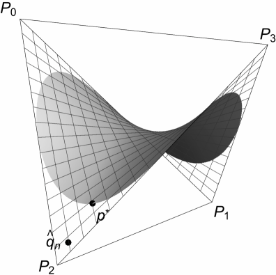
Figure 2: Geometry of two-dimensional quantum state tomography. The set ${\mathcal{B}}$ of physically valid states (deformed grayish disk) is a subset of the two-dimensional manifold ${\mathcal{P}}({\Omega})^{\otimes 2}$ of independent distributions (ruled surface) embedded in the three-dimensional probability simplex ${\mathcal{P}}({\Omega}^{2})$ (convex hull of $\{P_{0},P_{1},P_{2},P_{3}\}$). The maximum likelihood estimator $p^{*}$ is the point in ${\mathcal{B}}$ that is “closest” from the empirical distribution $\hat{q}_{n}$ as measured by the Kullback-Leibler divergence.

In order to get a better understanding of the above-mentioned difficulty, let us consider the case when $k=2$: this situation may be interpreted as the quantum state tomography restricted to the ${\xi}_{1}{\xi}_{2}$-plane. Fig. 2 depicts the relationship between ${\mathcal{P}}({\Omega}^{2})$ and ${\mathcal{P}}({\Omega})^{\otimes 2}$, as well as the subset ${\mathcal{B}}$ that corresponds to the quantum state space ${\mathcal{S}}({\mathbb{C}}^{2})$. The statistical manifold ${\mathcal{P}}({\Omega}^{2})$ is a 3-dimensional simplex represented by the convex hull of four points $P_{0}$, $P_{1}$, $P_{2}$, and $P_{3}$, each corresponding to the ${\delta}$-measure on the events $(+1,+1)$, $(+1,-1)$, $(-1,+1)$, and $(-1,-1)$, respectively. The ruled surface embedded in the simplex corresponds to the submanifold ${\mathcal{P}}({\Omega})^{\otimes 2}$ of independent distributions, and the deformed grayish disk lying on the ruled surface represents the subset ${\mathcal{B}}$ of physically valid states satisfying $({\xi}_{1})^{2}+({\xi}_{2})^{2}\leq 1$. Now suppose that the empirical distribution $\hat{q}_{n}\in{\mathcal{P}}({\Omega})^{\otimes 2}$ has fallen outside ${\mathcal{B}}$. The MLE $p^{*}$ is then given by the point on ${\mathcal{B}}$ that is “closest” from $\hat{q}_{n}$ as measured by the Kullback-Leibler divergence. Since the ruled surface ${\mathcal{P}}({\Omega})^{\otimes 2}$ is embedded in the simplex ${\mathcal{P}}({\Omega}^{2})$ as a “curved” surface, the $\nabla^{(m)}$-geodesic (straight line) connecting $\hat{q}_{n}$ and $p^{*}$ in ${\mathcal{P}}({\Omega}^{2})$ does not stay within ${\mathcal{P}}({\Omega})^{\otimes 2}$. Recall that there is a one-to-one correspondence between the set ${\mathcal{P}}({\Omega})^{\otimes 2}$ of independent distributions and the Stokes parameter space $(-1,1)^{2}$. Thus, the $\nabla^{(m)}$-geodesic connecting $\hat{q}_{n}$ and $p^{*}$ in ${\mathcal{P}}({\Omega}^{2})$ has no direct counterpart in the Stokes parameter space.

This difficulty can be surmounted by introducing a dualistic structure $(\overline{g},\overline{\nabla}^{(e)},\overline{\nabla}^{(m)})$ on the submanifold ${\mathcal{P}}({\Omega})^{\otimes k}$ as the restriction of the dualistic structure $(g,\nabla^{(e)},\nabla^{(m)})$ of the ambient statistical manifold ${\mathcal{P}}({\Omega}^{k})$ onto $P({\Omega})^{\otimes k}$. Since ${\mathcal{P}}({\Omega})^{\otimes k}$ is a $\nabla^{(e)}$-autoparallel submanifold of ${\mathcal{P}}({\Omega}^{k})$, ${\mathcal{P}}({\Omega})^{\otimes k}$ is automatically dually flat with respect to the induced structure $(\overline{g},\overline{\nabla}^{(e)},\overline{\nabla}^{(m)})$, and the parameters $\overline{\theta}$ and $\overline{\eta}$ defined by (7) and (9) form mutually dual $\overline{\nabla}^{(e)}$- and $\overline{\nabla}^{(m)}$-affine coordinate systems of ${\mathcal{P}}({\Omega})^{\otimes k}$. Let us denote the canonical $\overline{\nabla}^{(m)}$-divergence on ${\mathcal{P}}({\Omega})^{\otimes k}$ by $\overline{D}(p\|q)$. Note that the canonical $\nabla^{(m)}$-divergence on the ambient manifold ${\mathcal{P}}({\Omega}^{k})$ is nothing but the Kullback-Leibler divergence $D(p\|q)$. The key observation is the following

Lemma 3.

For any $p,q\in{\mathcal{P}}({\Omega})^{\otimes k}$, we have

$$\overline{D}(p\|q)=D(p\|q).$$

Proof.

The assertion has been proved under a more general setting in FujiwaraAmari:1995 ; however, we shall give an alternative proof for the sake of later discussion. Let $\overline{\theta}=({\theta}^{1},\dots,{\theta}^{k})$ and $\overline{\eta}=({\eta}_{1},\dots,{\eta}_{k})$ be mutually dual affine coordinate systems of ${\mathcal{P}}({\Omega})^{\otimes k}$ defined by (7) and (9), respectively. By extending these coordinate systems, we construct mutually dual $\nabla^{(e)}$- and $\nabla^{(m)}$-affine coordinate systems

$${\theta}=({\theta}^{1},\dots,{\theta}^{k};\,{\theta}^{k+1},\dots,{\theta}^{d})$$ (12)

and

$${\eta}=({\eta}_{1},\dots,{\eta}_{k};\,{\eta}_{k+1},\dots,{\eta}_{d})$$ (13)

of ${\mathcal{P}}({\Omega}^{k})$, with $d:=2^{k}-1$, such that the $\nabla^{(e)}$-autoparallel submanifold ${\mathcal{P}}({\Omega})^{\otimes k}$ corresponds to the points satisfying

$$({\theta}^{k+1},\dots,{\theta}^{d})=(0,\dots,0).$$ (14)

Furthermore, let $\psi({\theta})$ and $\varphi({\eta})$ be the dual potentials for the dual affine coordinate systems ${\theta}$ and ${\eta}$ of ${\mathcal{P}}({\Omega}^{k})$ satisfying

$$\psi({\theta})+\varphi({\eta})-{\theta}\cdot{\eta}=0,$$ (15)

where $\cdot$ denotes the standard inner product, and

$$\psi(\overline{\theta};\,0,\dots,0)=\overline{\psi}(\overline{\theta}),$$ (16)

where $\overline{\psi}(\overline{\theta})$ is the potential function on ${\mathcal{P}}({\Omega})^{\otimes k}$ defined by (8). Note that the dual potential function $\overline{\varphi}(\overline{\eta})$ on ${\mathcal{P}}({\Omega})^{\otimes k}$ is defined by

$$\overline{\varphi}(\overline{\eta}):=\overline{\theta}\cdot\overline{\eta}-\overline{\psi}(\overline{\theta}).$$ (17)

Now, since the Kullback-Leibler divergence $D(p\|q)$ is the $\nabla^{(m)}\,(=\nabla^{(e)*})$-divergence, we have

$$D(p\|q) = \psi({\theta}(q))+\varphi({\eta}(p))-{\theta}(q)\cdot{\eta}(p)$$

$$= \psi({\theta}(q))+\{{\theta}(p)\cdot{\eta}(p)-\psi({\theta}(p))\}-{\theta}(q)\cdot{\eta}(p)$$

$$= \psi({\theta}(q))-\psi({\theta}(p))+\{{\theta}(p)-{\theta}(q)\}\cdot{\eta}(p)$$

where ${\theta}(q)$, for instance, stands for the ${\theta}$-coordinate of the point $q\in{\mathcal{P}}({\Omega}^{k})$, and the identity (15) was used in the second equality. Furthermore, since both $p$ and $q$ belong to the submanifold ${\mathcal{P}}({\Omega})^{\otimes k}$, we have

$$D(p\|q) = \overline{\psi}(\overline{\theta}(q))-\overline{\psi}(\overline{\theta}(p))+(\overline{\theta}(p)-\overline{\theta}(q);\,0,\dots,0)\cdot{\eta}(p)$$

$$= \overline{\psi}(\overline{\theta}(q))-\overline{\psi}(\overline{\theta}(p))+\{\overline{\theta}(p)-\overline{\theta}(q)\}\cdot\overline{\eta}(p)$$

$$= \overline{\psi}(\overline{\theta}(q))-\{\overline{\theta}(p)\cdot\overline{\eta}(p)-\overline{\varphi}(\overline{\eta}(p))\}+\{\overline{\theta}(p)-\overline{\theta}(q)\}\cdot\overline{\eta}(p)$$

$$= \overline{\psi}(\overline{\theta}(q))+\overline{\varphi}(\overline{\eta}(p))-\overline{\theta}(q)\cdot\overline{\eta}(p)$$

$$= \overline{D}(p\|q).$$

Here, the first equality is due to (14) and (16), and the third due to (17). This proves the claim. ∎

It follows from Lemma 3 that the MLE (11) can be rewritten as

$$p^{*}=\mathop{\rm arg~{}min}\limits_{p\in{\mathcal{B}}}\;\overline{D}(\hat{q}_{3N}\|p).$$ (18)

This relation allows us to interpret the MLE $p^{*}$ in terms of the intrinsic geometry of the manifold ${\mathcal{P}}({\Omega})^{\otimes 3}$, without reference to the ambient manifold ${\mathcal{P}}({\Omega}^{3})$. To be specific, the MLE $p^{*}$ is the $\overline{\nabla}^{(m)}$-projection from $\hat{q}_{3N}$ to ${\mathcal{B}}$ in ${\mathcal{P}}({\Omega})^{\otimes 3}$, and the $\overline{\nabla}^{(m)}$-geodesic connecting $\hat{q}_{3N}$ and $p^{*}$ stays (of course!) within ${\mathcal{P}}({\Omega})^{\otimes 3}$.

II.3 Relation between ${\mathcal{P}}({\Omega})^{\otimes k}$ and $(-1,1)^{k}$

In the previous subsection, we interpreted the projection $\hat{q}_{3N}\mapsto p^{*}$ using an intrinsic geometry of ${\mathcal{P}}({\Omega})^{\otimes 3}$. In this subsection, we further interpret the process of finding the MLE using an intrinsic geometry of the Stokes parameter space $(-1,1)^{3}$.

Firstly, we recall that the coordinate system $\overline{\eta}=({\eta}_{i})$ of ${\mathcal{P}}({\Omega})^{\otimes k}$ and the coordinate system ${\xi}=({\xi}_{i})$ of $(-1,1)^{k}$ are related by (9), i.e.,

$${\eta}_{i}=\frac{1+{\xi}_{i}}{2}.$$

This correspondence establishes a diffeomorphism $f:(-1,1)^{k}\to{\mathcal{P}}({\Omega})^{\otimes k}$. Secondly, we introduce a Riemannian metric $\tilde{g}$ on $(-1,1)^{k}$ by

$$\tilde{g}_{p}(X,Y):=\overline{g}_{f(p)}(f_{*}X,f_{*}Y),\qquad\left(p\in(-1,1)^{k}\right)$$

where $\overline{g}$ is the Fisher metric on ${\mathcal{P}}({\Omega})^{\otimes k}$, and $f_{*}$ is the differential map of $f$. Thirdly, we introduce an affine connection $\tilde{\nabla}^{(m)}$ on $(-1,1)^{k}$ such that the coordinate system ${\xi}=({\xi}_{i})$ becomes $\tilde{\nabla}^{(m)}$-affine. This is nothing but the Euclidean connection induced from the natural affine structure of the ambient space ${\mathbb{R}}^{k}$. Finally, we introduce another affine connection $\tilde{\nabla}^{(e)}$ on $(-1,1)^{k}$ such that it satisfies the duality

$$X\tilde{g}(Y,Z)=\tilde{g}(\tilde{\nabla}^{(e)}_{X}Y,Z)+\tilde{g}(Y,\tilde{\nabla}^{(m)}_{X}Z).$$

In this way, we can regard the space $(-1,1)^{k}$ as a dually flat statistical manifold endowed with the dualistic structure $(\tilde{g},\tilde{\nabla}^{(e)},\tilde{\nabla}^{(m)})$.

Let us calculate the metric $\tilde{g}$ explicitly. From the relation (6), we have

$$\frac{\partial}{\partial{\xi}_{i}}\log p_{\xi}({\omega})=\frac{\partial}{\partial{\xi}_{i}}\log p_{{\xi}_{i}}({\omega}_{i})=\left\{\begin{array}[]{ll}\displaystyle\frac{1}{1+{\xi}_{i}},&({\omega}_{i}=+1)\\ \\ \displaystyle\frac{-1}{1-{\xi}_{i}},&({\omega}_{i}=-1)\end{array}\right..$$

Consequently,

$$\tilde{g}_{p_{\xi}}\left(\frac{\partial}{\partial{\xi}_{i}},\frac{\partial}{\partial{\xi}_{i}}\right) = \sum_{{\omega}\in{\Omega}^{k}}p_{\xi}({\omega})\left(\frac{\partial}{\partial{\xi}_{i}}\log p_{\xi}({\omega})\right)^{2}$$

$$= \frac{1+{\xi}_{i}}{2}\left(\frac{1}{1+{\xi}_{i}}\right)^{2}+\frac{1-{\xi}_{i}}{2}\left(\frac{-1}{1-{\xi}_{i}}\right)^{2}$$

$$= \frac{1}{1-({\xi}_{i})^{2}},$$

and for $i\neq j$,

$$\tilde{g}_{p_{\xi}}\left(\frac{\partial}{\partial{\xi}_{i}},\frac{\partial}{\partial{\xi}_{j}}\right) = \sum_{{\omega}\in{\Omega}^{k}}p_{\xi}({\omega})\left(\frac{\partial}{\partial{\xi}_{i}}\log p_{\xi}({\omega})\right)\left(\frac{\partial}{\partial{\xi}_{j}}\log p_{\xi}({\omega})\right)$$

$$= \left[\sum_{{\omega}_{i}\in{\Omega}}p_{{\xi}_{i}}({\omega}_{i})\left(\frac{\partial}{\partial{\xi}_{i}}\log p_{{\xi}_{i}}({\omega}_{i})\right)\right]\left[\sum_{{\omega}_{j}\in{\Omega}}p_{{\xi}_{j}}({\omega}_{j})\left(\frac{\partial}{\partial{\xi}_{j}}\log p_{{\xi}_{j}}({\omega}_{j})\right)\right]$$

$$= \left[\sum_{{\omega}_{i}\in{\Omega}}\left(\frac{\partial}{\partial{\xi}_{i}}p_{{\xi}_{i}}({\omega}_{i})\right)\right]\left[\sum_{{\omega}_{j}\in{\Omega}}\left(\frac{\partial}{\partial{\xi}_{j}}p_{{\xi}_{j}}({\omega}_{j})\right)\right]$$

$$= 0.$$

In summary,

$$\tilde{g}_{p_{\xi}}\left(\frac{\partial}{\partial{\xi}_{i}},\frac{\partial}{\partial{\xi}_{j}}\right)=\frac{{\delta}_{ij}}{1-({\xi}_{i})^{2}}.$$ (19)

When $k=3$, this is identical to (2).

Now let us proceed to investigating the relationship between $(-1,1)^{k}$ and ${\mathcal{P}}({\Omega})^{\otimes k}$. We say two statistical manifolds $(\tilde{M},\tilde{g},\tilde{\nabla},\tilde{\nabla}^{*})$ and $(\overline{M},\overline{g},\overline{\nabla},\overline{\nabla}^{*})$ are statistically isomorphic, or simply isostatistic, if there is a diffeomorphism $f:\tilde{M}\to\overline{M}$ such that

$$\tilde{g}_{p}(X,Y)=\overline{g}_{f(p)}(f_{*}X,f_{*}Y),\quad f_{*}(\tilde{\nabla}_{X}Y)_{p}=(\overline{\nabla}_{f_{*}X}f_{*}Y)_{f(p)},\quad f_{*}(\tilde{\nabla}^{*}_{X}Y)_{p}=(\overline{\nabla}^{*}_{f_{*}X}f_{*}Y)_{f(p)}$$

holds for all $p\in\tilde{M}$ and vector fields $X,Y$ on $\tilde{M}$.

Lemma 4.

The manifolds $((-1,1)^{k},\tilde{g},\tilde{\nabla}^{(e)},\tilde{\nabla}^{(m)})$ and $({\mathcal{P}}({\Omega})^{\otimes k},\overline{g},\overline{\nabla}^{(e)},\overline{\nabla}^{(m)})$ are isostatistic.

Proof.

Let $f:(-1,1)^{k}\to{\mathcal{P}}({\Omega})^{\otimes k}$ be the diffeomorphism defined above. Then

$$\tilde{g}_{p}(X,Y)=\overline{g}_{f(p)}(f_{*}X,f_{*}Y)$$

is obvious from the definition. Since ${\xi}$ is a $\tilde{\nabla}^{(m)}$-affine coordinate system of $(-1,1)^{k}$ and ${\eta}$ is a $\overline{\nabla}^{(m)}$-affine coordinate system of ${\mathcal{P}}({\Omega})^{\otimes k}$,

$$f_{*}(\tilde{\nabla}^{(m)}_{\partial^{i}}\partial^{j})_{p}=0=(\overline{\nabla}^{(m)}_{f_{*}\partial^{i}}f_{*}\partial^{j})_{f(p)}$$

for all $i,j\in\{1,\dots,k\}$, where $\partial^{i}:=\partial/\partial{\xi}_{i}$. Finally, since $f$ is a diffeomorphism,

$$\tilde{g}_{p}(\tilde{\nabla}^{(e)}_{X}Y,Z) = X_{p}\,\tilde{g}(Y,Z)-\tilde{g}_{p}(Y,\tilde{\nabla}^{(m)}_{X}Z)$$

$$= (f_{*}X)_{f(p)}\overline{g}(f_{*}Y,f_{*}Z)-\overline{g}_{f(p)}(f_{*}Y,\overline{\nabla}^{(m)}_{f_{*}X}f_{*}Z)$$

$$= \overline{g}_{f(p)}(\overline{\nabla}^{(e)}_{f_{*}X}f_{*}Y,f_{*}Z),$$

which leads us to

$$f_{*}(\tilde{\nabla}^{(e)}_{X}Y)_{p}=(\overline{\nabla}^{(e)}_{f_{*}X}f_{*}Y)_{f(p)}.$$

This proves the assertion. ∎

Returning to the quantum state tomography, Lemma 4 implies that the Stokes parameter space $(-1,1)^{3}$ endowed with the dualistic structure $(\tilde{g},\tilde{\nabla}^{(e)},\tilde{\nabla}^{(m)})$ can be identified with the statistical manifold ${\mathcal{P}}({\Omega})^{\otimes 3}$ of product distributions. Combining this fact with the results in the previous subsection, we have the following

Corollary 5.

The MLE ${\xi}^{*}$ that satisfies $p^{*}=p_{{\xi}^{*}}$ is the $\tilde{\nabla}^{(m)}$-projection from the temporal estimate $\hat{\xi}$ to the Bloch ball $B$ in the Stokes parameter space $(-1,1)^{3}$.

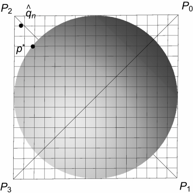
Figure 3: Geometry of two-dimensional quantum state tomography as seen from the top of Fig. 2. This space is isostatistic to the Stokes parameter space $(-1,1)^{2}$, and the grayish disk corresponds to (a slice of) the Bloch ball representing the quantum state space ${\mathcal{S}}({\mathbb{C}}^{2})$. In the space ${\mathcal{P}}({\Omega}^{2})$ of probability distributions, the MLE $p^{*}$ was the point in ${\mathcal{B}}$ that is “closest” from the empirical distribution $\hat{q}_{n}$ as measured by the Kullback-Leibler divergence. Likewise, in the Stokes parameter space, the MLE ${\xi}^{*}$ that satisfies $p^{*}=p_{{\xi}^{*}}$ is the $\tilde{\nabla}^{(m)}$-projection from the temporal estimate $\hat{\xi}$ to the Bloch ball $B$.

Incidentally, it should be noted that the isostatistic correspondence between $(-1,1)^{k}$ and ${\mathcal{P}}({\Omega})^{\otimes k}$ can be visualized by “looking at ${\mathcal{P}}({\Omega})^{\otimes k}$ from the top.” For instance, when $k=2$, the space ${\mathcal{P}}({\Omega})^{\otimes 2}$ was the ruled surface depicted in Fig. 2. If we look at the space from the top (see Fig. 3), we can find (a two-dimensional slice of) the Bloch ball embedded in the Stokes parameter space. This is because the diffeomorphism $f:(-1,1)^{k}\to{\mathcal{P}}({\Omega})^{\otimes k}$ is given by the affine transformation (9). Recall that, in the proof of Lemma 3, we introduced a $\nabla^{(m)}$-affine coordinate system ${\eta}=({\eta}_{1},\dots,{\eta}_{k};\,{\eta}_{k+1},\dots,{\eta}_{d})$ of ${\mathcal{P}}({\Omega}^{k})$, the first $k$ components of which gave a $\overline{\nabla}^{(m)}$-affine coordinate system of ${\mathcal{P}}({\Omega})^{\otimes k}$. If we look at the space ${\mathcal{P}}({\Omega}^{k})$ from a certain angle in such a way that the remaining $(d-k)$-components $({\eta}_{k+1},\dots,{\eta}_{d})$ are “squashed,” then we can visualize the shape of ${\mathcal{P}}({\Omega})^{\otimes k}$, which is affinely isomorphic to $(-1,1)^{k}$. This is the underlying mechanism behind Fig. 3.

II.4 Computation of MLE

Let $\hat{\xi}$ be the temporal estimate defined by (1), i.e.,

$$\hat{\xi}=(\hat{\xi}_{1},\hat{\xi}_{2},\hat{\xi}_{3}):=\left(\frac{n_{1}^{+}-n_{1}^{-}}{N},\;\frac{n_{2}^{+}-n_{2}^{-}}{N},\;\frac{n_{3}^{+}-n_{3}^{-}}{N}\right).$$

By a slight abuse of terminology, we shall call $\hat{\xi}$ the empirical distribution on the Stokes parameter space. Suppose that the empirical distribution $\hat{\xi}$ has fallen outside the Bloch ball $B$. Let ${\xi}^{*}=({\xi}_{1}^{*},{\xi}^{*}_{2},{\xi}^{*}_{3})$ be a point on the Bloch sphere $S$ in the Stokes parameter space. If ${\xi}^{*}$ is the MLE, then we see from Corollary 5 that the $\tilde{\nabla}^{(m)}$-geodesic (i.e., the straight line) connecting ${\xi}^{*}$ and $\hat{\xi}$ must be orthogonal to the Bloch sphere $S$ at ${\xi}^{*}$ with respect to the induced Riemannian metric $\tilde{g}$. Stated otherwise, the tangent vector $V$ of that geodesic at ${\xi}^{*}$, which is explicitly given by

$$V:=\sum_{i=1}^{3}(\hat{\xi}_{i}-{\xi}^{*}_{i})\left(\frac{\partial}{\partial{\xi}_{i}}\right)_{{\xi}^{*}},$$ (20)

satisfies the orthogonality

$$\tilde{g}_{{\xi}^{*}}(V,X)=0$$ (21)

for all tangent vectors $X\in T_{{\xi}^{*}}S$ of the Bloch sphere $S$ at ${\xi}^{*}$. The MLE ${\xi}^{*}$ can be obtained as a solution of the equation (21).

Here we propose a method of computing the MLE ${\xi}^{*}$. In Euclidean geometry, the position vector $\overrightarrow{{\xi}}=({\xi}_{1},{\xi}_{2},{\xi}_{3})$ of a point ${\xi}$ on the unit sphere $S$ is normal to $S$, in that they satisfy

$$\sum_{i=1}^{3}{\xi}_{i}X_{i}=0$$ (22)

for all tangent vectors $\overrightarrow{X}=(X_{1},X_{2},X_{3})\in T_{\xi}S$ of $S$. Using the relation (22), we can find a tangent vector $\overrightarrow{n}$ at ${\xi}\in S$ that is normal to $S$ with respect to the metric $\tilde{g}$. Let

$$\overrightarrow{n}=\sum_{i=1}^{3}a_{i}\left(\frac{\partial}{\partial{\xi}_{i}}\right)_{{\xi}}$$

and let us represent a tangent vector $\overrightarrow{X}\in T_{\xi}S$ of $S$ as

$$\overrightarrow{X}=\sum_{i=1}^{3}X_{i}\left(\frac{\partial}{\partial{\xi}_{i}}\right)_{{\xi}}.$$

The orthogonality with respect to $\tilde{g}$ is then written as

$$\tilde{g}_{\xi}(\overrightarrow{n},\overrightarrow{X}) = \sum_{i,j=1}^{3}a_{i}X_{j}\,\tilde{g}_{\xi}\left(\frac{\partial}{\partial{\xi}_{i}},\frac{\partial}{\partial{\xi}_{j}}\right)$$

$$= \sum_{i,j=1}^{3}a_{i}X_{j}\,\frac{{\delta}_{ij}}{1-({\xi}_{i})^{2}}$$

$$= \sum_{i=1}^{3}\frac{a_{i}}{1-({\xi}_{i})^{2}}\,X_{i}$$

$$= 0.$$

In the second equality, we used the explicit formula (19) for the Riemannian metric $\tilde{g}$. Comparing this relation with (22), we see that the choice

$$a_{i}:={\xi}_{i}\left(1-({\xi}_{i})^{2}\right)$$

gives a desired tangent vector $\overrightarrow{n}$ that is normal to $S$ at ${\xi}$ with respect to $\tilde{g}$.

The condition (21) for the MLE ${\xi}^{*}$ is now restated that the tangent vector (20) of the $\tilde{\nabla}^{(m)}$-geodesic should be parallel to the normal vector $\overrightarrow{n}$ at ${\xi}^{*}$, so that there is a positive real number ${\lambda}$ such that $\overrightarrow{n}={\lambda}V$, or equivalently,

$${\xi}^{*}_{i}\left(1-({\xi}^{*}_{i})^{2}\right)={\lambda}(\hat{\xi}_{i}-{\xi}^{*}_{i}),\qquad(i\in\{1,2,3\}).$$

The MLE ${\xi}^{*}$ is obtained by the unique solution of these equations together with the normalizing condition

$$\sum_{i=1}^{3}({\xi}^{*}_{i})^{2}=1,$$

and the positivity condition ${\lambda}>0$. The proof of Theorem 1 is now complete.

III Proof of Theorem 2

Generalizing Theorem 1 to Theorem 2 is, in a sense, straightforward: we need only change the metric $\tilde{g}$ on $(-1,1)^{3}$ from (2) to (3) in the proof of Lemma 4, based on the fact that the Fisher information of i.i.d. extensions of a statistical model increases linearly in the degree of extensions. However, we here give an alternative proof, in order to reveal a different aspect of the quantum state tomography.

Let us consider the following experiment: One of the three observables ${\sigma}_{1},{\sigma}_{2}$, and ${\sigma}_{3}$ is chosen at random with probability $s_{1},s_{2}$, and $(1-s_{1}-s_{2})$, respectively, and measure the chosen observable to yield an outcome either $+1$ or $-1$. We could estimate the unknown state ${\rho}\in{\mathcal{S}}({\mathbb{C}}^{2})$ by repeating this randomized experiment. In particular, if $s_{1}=s_{2}=\frac{1}{3}$, this experiment is asymptotically equivalent to the standard quantum state tomography because of the law of large numbers. We shall call such an experiment a randomized tomography Yamagata:2011 .

The sample space ${\Omega}$ for a randomized tomography is

$${\Omega}=\{({\sigma}_{1},+1),({\sigma}_{1},-1),({\sigma}_{2},+1),({\sigma}_{2},-1),({\sigma}_{3},+1),({\sigma}_{3},-1)\}.$$

If the unknown state is specified by the Stokes parameters ${\xi}=({\xi}_{1},{\xi}_{2},{\xi}_{3})$, then the corresponding probability distribution on ${\Omega}$ is given by the probability vector

$$p_{(s,{\xi})}:=\left(s_{1}\frac{1+{\xi}_{1}}{2},s_{1}\frac{1-{\xi}_{1}}{2},s_{2}\frac{1+{\xi}_{2}}{2},s_{2}\frac{1-{\xi}_{1}}{2},(1-s_{1}-s_{2})\frac{1+{\xi}_{3}}{2},(1-s_{1}-s_{2})\frac{1-{\xi}_{3}}{2}\right),$$

where $s:=(s_{1},s_{2})$ with the domain

$$D:=\{(s_{1},s_{2})\;|\;s_{1}>0,\;s_{2}>0,\;1-s_{1}-s_{2}>0\}.$$

Note that the family

$$\{p_{(s,{\xi})}\;|\;s\in D,\,{\xi}\in(-1,1)^{3}\}$$

is identical to the five-dimensional probability simplex ${\mathcal{P}}({\Omega})$, and the parameters $(s,{\xi})$ form a coordinate system of ${\mathcal{P}}({\Omega})$. Since we are interested in estimating only the Stokes parameters ${\xi}=({\xi}_{1},{\xi}_{2},{\xi}_{3})$, the remaining parameters $s=(s_{1},s_{2})$ are regarded as nuisance parameters LehmanCasella ; AmariLN in the terminology of statistics. In what follows, ${\mathcal{P}}({\Omega})$ is regarded as a statistical manifold endowed with the dualistic structure $(g,\nabla^{(e)},\nabla^{(m)})$, where $g$ is the Fisher metric, and $\nabla^{(e)}$ and $\nabla^{(m)}$ are the exponential and mixture connections.

Let us consider the following submanifolds of ${\mathcal{P}}({\Omega})$:

$$M(s):=\{p_{(s,{\xi})}\;|\;{\xi}\in(-1,1)^{3}\}$$

for each $s\in D$, and

$$E({\xi}):=\{p_{(s,{\xi})}\;|\;s\in D\}$$

for each ${\xi}\in(-1,1)^{3}$. Since $M(s)$ and $E({\xi})$ are convex subsets of ${\mathcal{P}}({\Omega})$, they are $\nabla^{(m)}$-autoparallel. The following Lemma is the key to the estimation of ${\xi}$ under the nuisance parameters $s$.

Lemma 6.

For each ${\xi}\in(-1,1)^{3}$, the submanifold $E({\xi})$ is $\nabla^{(e)}$-autoparallel. Furthermore, for each $s\in D$ and ${\xi}\in(-1,1)^{3}$, the submanifolds $M(s)$ and $E({\xi})$ are mutually orthogonal with respect to the Fisher metric $g$.

Proof.

Let us change the coordinate system $(s,{\xi})=(s_{1},s_{2},{\xi}_{1},{\xi}_{2},{\xi}_{3})$ into

$${\eta}:=({\eta}_{1},\,{\eta}_{2},\,{\eta}_{3},\,{\eta}_{4},\,{\eta}_{5}):=(s_{1},\,s_{2},\,s_{1}{\xi}_{1},\,s_{2}{\xi}_{2},\,(1-s_{1}-s_{2}){\xi}_{3}).$$

With this coordinate transformation, the probability vector $p_{(s,{\xi})}$ is rewritten as

$$p_{\eta}:=\left(\frac{{\eta}_{1}+{\eta}_{3}}{2},\frac{{\eta}_{1}-{\eta}_{3}}{2},\frac{{\eta}_{2}+{\eta}_{4}}{2},\frac{{\eta}_{2}-{\eta}_{4}}{2},\frac{1-{\eta}_{1}-{\eta}_{2}+{\eta}_{5}}{2},\frac{1-{\eta}_{1}-{\eta}_{2}-{\eta}_{5}}{2}\right).$$

We see from this expression that the coordinate system ${\eta}:=({\eta}_{i})_{1\leq i\leq 5}$ is $\nabla^{(m)}$-affine. The potential function for ${\eta}$ is given by the negative entropy

$$\varphi({\eta}):=\sum_{{\omega}\in{\Omega}}p_{\eta}({\omega})\log p_{\eta}({\omega}),$$

and the dual $\nabla^{(e)}$-affine coordinate system ${\theta}=({\theta}^{i})_{1\leq i\leq 5}$ is given by

$${\theta}^{i}:=\frac{\partial\varphi}{\partial{\eta}_{i}}.$$

By direct computation, we have

$${\theta}^{1}=\frac{1}{2}\log\frac{({\eta}_{1}+{\eta}_{3})({\eta}_{1}-{\eta}_{3})}{(1-{\eta}_{1}-{\eta}_{2}+{\eta}_{5})(1-{\eta}_{1}-{\eta}_{2}-{\eta}_{5})}=\frac{1}{2}\log\left[\left(\frac{s_{1}}{1-s_{1}-s_{2}}\right)^{2}\frac{1-({\xi}_{1})^{2}}{1-({\xi}_{3})^{2}}\right],$$

$${\theta}^{2}=\frac{1}{2}\log\frac{({\eta}_{2}+{\eta}_{4})({\eta}_{2}-{\eta}_{4})}{(1-{\eta}_{1}-{\eta}_{2}+{\eta}_{5})(1-{\eta}_{1}-{\eta}_{2}-{\eta}_{5})}=\frac{1}{2}\log\left[\left(\frac{s_{2}}{1-s_{1}-s_{2}}\right)^{2}\frac{1-({\xi}_{2})^{2}}{1-({\xi}_{3})^{2}}\right],$$

$${\theta}^{3}=\frac{1}{2}\log\frac{{\eta}_{1}+{\eta}_{3}}{{\eta}_{1}-{\eta}_{3}}=\frac{1}{2}\log\frac{1+{\xi}_{1}}{1-{\xi}_{1}},$$

$${\theta}^{4}=\frac{1}{2}\log\frac{{\eta}_{2}+{\eta}_{4}}{{\eta}_{2}-{\eta}_{4}}=\frac{1}{2}\log\frac{1+{\xi}_{2}}{1-{\xi}_{2}},$$

$${\theta}^{5}=\frac{1}{2}\log\frac{1-{\eta}_{1}-{\eta}_{2}+{\eta}_{5}}{1-{\eta}_{1}-{\eta}_{2}-{\eta}_{5}}=\frac{1}{2}\log\frac{1+{\xi}_{3}}{1-{\xi}_{3}}.$$

Thus, fixing ${\xi}$ is equivalent to fixing the three coordinates $({\theta}^{3},{\theta}^{4},{\theta}^{5})$, and the submanifold $E({\xi})$ is generated by changing the remaining two parameters $({\theta}^{1},{\theta}^{2})$. This implies that $E({\xi})$ is $\nabla^{(e)}$-autoparallel, proving the first part of the claim.

To prove the second part, let us introduce a mixed coordinate system AmariNagaoka

$$({\eta}_{1},{\eta}_{2};\,{\theta}^{3},{\theta}^{4},{\theta}^{5})$$

of ${\mathcal{S}}({\Omega})$. Since $({\eta}_{1},{\eta}_{2})=(s_{1},s_{2})$, the submanifold $M(s)$ is rewritten as

$$M(s)=\{p_{(s,{\xi})}\;|\;\mbox{$({\eta}_{1},{\eta}_{2})$ are fixed and $({\theta}^{3},{\theta}^{4},{\theta}^{5})$ are arbitrary}\}.$$

On the other hand, as was seen in the above, the submanifold $E({\xi})$ is rewritten as

$$E({\xi})=\{p_{(s,{\xi})}\;|\;\mbox{$({\theta}^{3},{\theta}^{4},{\theta}^{5})$ are fixed and $({\eta}_{1},{\eta}_{2})$ are arbitrary}\}.$$

Thus the general orthogonality relation

$$g\left(\frac{\partial}{\partial{\theta}^{i}},\frac{\partial}{\partial{\eta}_{j}}\right)={\delta}_{i}^{j}$$

proves that $M(s)$ and $E({\xi})$ are orthogonal to each other. ∎

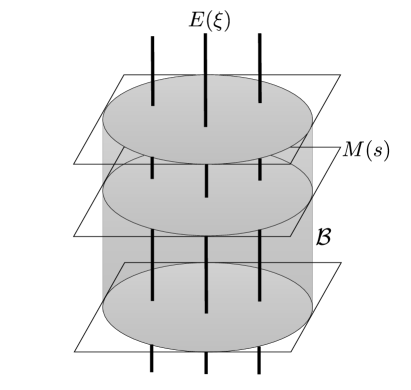
Figure 4: Mutually orthogonal dualistic foliation of ${\mathcal{P}}({\Omega})$ based on $M(s)$ and $E({\xi})$. Each section $M(s)$ is affinely isomorphic to the Stokes parameter space $(-1,1)^{3}$. The grayish cylindrical area indicates the subset ${\mathcal{B}}=\{p_{(s,{\xi})}|s\in D,\,{\xi}\in B\}$ of ${\mathcal{P}}({\Omega})$ that corresponds to the Bloch ball $B$. In particular, for each $s\in D$, the intersection $M(s)\cap{\mathcal{B}}$ is affinely isomorphic to the Bloch ball $B$.

Lemma 6 implies that the manifold ${\mathcal{P}}({\Omega})$ is decomposed into a mutually orthogonal dualistic foliation based on the submanifolds $M(s)$ and $E({\xi})$, as illustrated in Fig. 4.

Let us get down to the problem of estimating the unknown Stokes parameters ${\xi}$ using the randomized tomography. Suppose that, among $N$ independent experiments of randomized tomography, the $i$th Pauli matrix ${\sigma}_{i}$ was measured $N_{i}$ times and obtained outcomes $+1$ and $-1$, each $n_{i}^{+}$ and $n_{i}^{-}$ times. Then a temporal estimate $(\hat{s},\hat{\xi})$ for the parameters $(s,{\xi})$ are

$$\hat{s}=\left(\frac{N_{1}}{N},\frac{N_{2}}{N}\right)$$

and

$$\hat{\xi}=\left(\frac{n_{1}^{+}-n_{1}^{-}}{N_{1}},\frac{n_{2}^{+}-n_{2}^{-}}{N_{2}},\frac{n_{3}^{+}-n_{3}^{-}}{N_{3}}\right).$$

If $\hat{\xi}$ has fallen outside the Bloch ball $B$, we may find a corrected estimate by the maximum likelihood method. First of all, the empirical distribution $\hat{q}_{N}\in{\mathcal{S}}({\Omega})$ is given by

$$\hat{q}_{N}:=p_{(\hat{s},\hat{\xi})}.$$

On the other hand, the Bloch ball $B$ in the Stokes parameter space $(-1,1)^{3}$ corresponds to the subset

$${\mathcal{B}}:=\{p_{(s,{\xi})}\;|\;s\in D,\;{\xi}\in B\}$$

of ${\mathcal{P}}({\Omega})$, (cf., Fig. 4). The MLE $p^{*}$ in ${\mathcal{P}}({\Omega})$ is then given by

$$p^{*}=\mathop{\rm arg~{}min}\limits_{p\in{\mathcal{B}}}D(\hat{q}_{N}\|p).$$ (23)

This is the $\nabla^{(m)}$-projection from the empirical distribution $\hat{q}_{N}$ to ${\mathcal{B}}$. A crucial observation is the following

Lemma 7.

The minimum in (23) is achieved on $M(\hat{s})\cap{\mathcal{B}}$.

Proof.

Let us take a point $p_{(s,{\xi})}\in{\mathcal{B}}$ arbitrarily. It then follows from the mutually orthogonal dualistic foliation of ${\mathcal{P}}({\Omega})$ established in Lemma 6 that

$$D(\hat{q}_{N}\|p_{(s,{\xi})}) = D(p_{(\hat{s},\hat{\xi})}\|p_{(s,{\xi})})$$

$$= D(p_{(\hat{s},\hat{\xi})}\|p_{(\hat{s},{\xi})})+D(p_{(\hat{s},{\xi})}\|p_{(s,{\xi})})$$

$$\geq D(p_{(\hat{s},\hat{\xi})}\|p_{(\hat{s},{\xi})}).$$

In the second equality, the generalized Pythagorean theorem was used. Consequently,

$$\min_{{\xi}\in B}D(p_{(\hat{s},\hat{\xi})}\|p_{(s,{\xi})})\geq\min_{{\xi}\in B}D(p_{(\hat{s},\hat{\xi})}\|p_{(\hat{s},{\xi})})$$

for all $s\in D$, and the lower bound is achieved if and only if $s=\hat{s}$. ∎

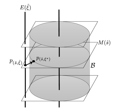
Figure 5: The maximum likelihood method in the framework of randomized tomography. Given a temporal estimate $(\hat{s},\hat{\xi})$ with $\hat{\xi}\notin B$, we can restrict ourselves to the slice $M(\hat{s})$ as the search space for the MLE $p^{*}$, and $p^{*}=p_{(\hat{s},{\xi}^{*})}$ is the $\nabla^{(m)}$-projection from the empirical distribution $p_{(\hat{s},\hat{\xi})}$ to ${\mathcal{B}}$ on the slice $M(\hat{s})$.

The geometrical implication of Lemma 7 is illustrated in Fig. 5. The MLE $p^{*}=p_{(\hat{s},{\xi}^{*})}$ is the $\nabla^{(m)}$-projection from the empirical distribution $p_{(\hat{s},\hat{\xi})}$ to ${\mathcal{B}}$ on the slice $M(\hat{s})$.

Now we are ready to prove Theorem 2. Suppose we are given a temporal estimate $(\hat{s},\hat{\xi})$ with $\hat{\xi}\notin B$. Due to Lemma 7, we can restrict ourselves to the slice $M(\hat{s})$ as the search space for the MLE $p^{*}$. Since the slice $M(\hat{s})$ is affinely isomorphic to the Stokes parameter space $(-1,1)^{3}$, we can introduce a dualistic structure $(\tilde{g},\tilde{\nabla}^{(e)},\tilde{\nabla}^{(m)})$ on $(-1,1)^{3}$ in the following way. Firstly, in a quite similar way to the derivation of (19), it is shown that the components of the Fisher metric $g$ on the section $M(\hat{s})$ with respect to the coordinate system ${\xi}=({\xi}_{1},{\xi}_{2},{\xi}_{3})$ are given by

$$g_{(\hat{s},{\xi})}\left(\frac{\partial}{\partial{\xi}_{i}},\frac{\partial}{\partial{\xi}_{j}}\right)=\frac{\hat{s}_{i}\,{\delta}_{ij}}{1-({\xi}_{i})^{2}},$$

where $\hat{s}_{3}:=1-\hat{s}_{1}-\hat{s}_{2}$. We identify this metric with $\tilde{g}$, i.e.,

$$\tilde{g}_{{\xi}}\left(\frac{\partial}{\partial{\xi}_{i}},\frac{\partial}{\partial{\xi}_{j}}\right):=\frac{\hat{s}_{i}\,{\delta}_{ij}}{1-({\xi}_{i})^{2}}.$$

Secondly, the mixture connection $\tilde{\nabla}^{(m)}$ is defined so that the coordinate system ${\xi}=({\xi}_{1},{\xi}_{2},{\xi}_{3})$ of $(-1,1)^{3}$ becomes $\tilde{\nabla}^{(m)}$-affine. Finally, the dual connection $\tilde{\nabla}^{(e)}$ is defined by the duality

$$\tilde{g}(\tilde{\nabla}^{(e)}_{X}Y,Z):=X\tilde{g}(Y,Z)-\tilde{g}(Y,\tilde{\nabla}^{(e)}_{X}Z).$$

It is shown, in a quite similar way to the proof of Lemma 4, that the statistical manifold $((-1,1)^{3},\tilde{g},\tilde{\nabla}^{(e)},\tilde{\nabla}^{(m)})$ is isostatistic to the manifold $M(s)$ with a dualistic structure defined by the restriction of $(g,\nabla^{(e)},\nabla^{(m)})$ to $M(s)$. Thus, the MLE ${\xi}^{*}$ in the Stokes parameter space is given by the $\tilde{\nabla}^{(m)}$-projection from $\hat{\xi}$ to the Bloch sphere $S$ with respect to the metric $\tilde{g}$. This proves the first part of Theorem 2. The remainder of Theorem 2 is proved in the same way as the corresponding part of Theorem 1.

   

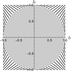
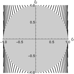
Figure 6: The trajectories of $\tilde{\nabla}^{(m)}$-projections on the ${\xi}_{1}{\xi}_{2}$-plane that give the MLE $p^{*}$ when $N_{1}:N_{2}=1:1$ (left), and $N_{1}:N_{2}=5:1$ (right). The change of ${\xi}_{1}$-coordinate relative to the change of ${\xi}_{2}$-coordinate along each trajectory is less noticeable in the right panel than in the left panel. This is because a tomography with $N_{1}/N_{2}=5$ provides us with more information about ${\xi}_{1}$, relative to ${\xi}_{2}$, as compared to that with $N_{1}/N_{2}=1$.

Fig. 6 demonstrates how the $\tilde{\nabla}^{(m)}$-projection is realized on the ${\xi}_{1}{\xi}_{2}$-plane of the Stokes parameter space: the left and right panels correspond to the cases when $N_{1}:N_{2}=1:1$ and $N_{1}:N_{2}=5:1$, respectively. The change of ${\xi}_{1}$-coordinate relative to the change of ${\xi}_{2}$-coordinate along each trajectory is less noticeable in the right panel than in the left panel. This is because a tomography with $N_{1}/N_{2}=5$ provides us with more information about ${\xi}_{1}$-coordinate, relative to ${\xi}_{2}$-coordinate, as compared to that with $N_{1}/N_{2}=1$.

IV Numerical demonstration

In this section, we devise a method of computing the MLE based on Theorem 2. Suppose we are given a temporal estimate

$$\hat{\xi}=(\hat{\xi}_{1},\hat{\xi}_{2},\hat{\xi}_{3}):=\left(\frac{n_{1}^{+}-n_{1}^{-}}{N_{1}},\;\frac{n_{2}^{+}-n_{2}^{-}}{N_{2}},\;\frac{n_{3}^{+}-n_{3}^{-}}{N_{3}}\right).$$

If $\|\hat{\xi}\|\leq 1$, then $\hat{\xi}$ already gives a valid estimate (in fact the MLE) for ${\xi}$. Otherwise, the estimate is corrected using the method stated in Theorem 2: the corrected estimate ${\xi}^{*}=({\xi}^{*}_{1},{\xi}^{*}_{2},{\xi}^{*}_{3})$ is the unique solution of the simultaneous equations

$${\xi}^{*}_{i}\left(1-({\xi}^{*}_{i})^{2}\right)={\lambda}\hat{s}_{i}\,(\hat{\xi}_{i}-{\xi}^{*}_{i}),\qquad(i\in\{1,2,3\})$$ (24)

and

$$({\xi}^{*}_{1})^{2}+({\xi}^{*}_{2})^{2}+({\xi}^{*}_{3})^{2}=1,$$ (25)

with ${\lambda}>0$.

Let us consider, for each $a\in(-1,1)$, the following cubic equation in $x$:

$$x(1-x^{2})={\mu}(a-x).$$

This equation has a unique solution

$$x=({\rm sgn}\,a)\frac{2\sqrt{{\mu}+1}}{\sqrt{3}}\cos\left[\frac{1}{3}\left(\pi+\arctan\sqrt{\frac{4({\mu}+1)^{3}}{27{\mu}^{2}a^{2}}-1}\right)\right]$$ (26)

in the interval $-1<x<1$. Let us denote the right-hand side of (26) as $x({\mu},a)$. Then the solution of each equation in (24) is given by ${\xi}^{*}_{i}=x({\lambda}\hat{s}_{i},\hat{\xi}_{i})$, and the norm condition (25) is reduced to

$$x({\lambda}\hat{s}_{1},\hat{\xi}_{1})^{2}+x({\lambda}\hat{s}_{2},\hat{\xi}_{2})^{2}+x({\lambda}\hat{s}_{3},\hat{\xi}_{3})^{2}=1.$$ (27)

This is an equation for a single variable ${\lambda}$. Let ${\lambda}^{*}$ be the unique positive solution of (27). Then the MLE is given by

$${\xi}^{*}_{i}=x({\lambda}^{*}\hat{s}_{i},\hat{\xi}_{i}),\qquad(i\in\{1,2,3\}).$$

In practice, the solution ${\lambda}^{*}$ cannot be obtained explicitly: thus, we must invoke numerical evaluation. For the sake of demonstration, we computed the MLE 1000 times on MATHEMATICA software version 10.4, using (i) FindRoot function to solve (27), and (ii) FindMaximun function to find the maximizer (4) directly, under the condition that $N_{1}=N_{2}=N_{3}$, starting from randomly generated initial points $(\hat{\xi}_{1},\hat{\xi}_{2},\hat{\xi}_{3})$ that fall outside the Bloch ball. The average computation time was 2.20313 [msec] for (i), and 21.6406 [msec] for (ii). As far as this demonstration is concerned, our method works very efficiently.

We note that the present method has been successfully applied to an experimental study using photonic qubits OkamotoOYFT:2016 .

V Conclusions

In the present paper, a statistically feasible method of data post-processing for the quantum state tomography was studied from an information geometrical point of view. Suppose that, among $N$ independent experiment, the $i$th Pauli matrix ${\sigma}_{i}$ was measured $N_{i}$ times and obtained outcomes $+1$ and $-1$, each $n^{+}_{i}$ and $n^{-}_{i}$ times. Then the space $(-1,1)^{3}$ of the Stokes parameter ${\xi}=({\xi}_{1},{\xi}_{2},{\xi}_{3})$ should be regarded as a Riemannian manifold endowed with a metric

$$g_{\xi}\left(\frac{\partial}{\partial{\xi}_{i}},\frac{\partial}{\partial{\xi}_{j}}\right)=\frac{\hat{s}_{i}\,{\delta}_{ij}}{1-({\xi}_{i})^{2}},$$

where $\hat{s}_{i}:=N_{i}/N$. Furthermore, if the temporal estimate

$$\hat{\xi}=\left(\frac{n^{+}_{1}-n^{-}_{1}}{N_{1}},\frac{n^{+}_{2}-n^{-}_{2}}{N_{2}},\frac{n^{+}_{3}-n^{-}_{3}}{N_{3}}\right)$$

for the parameter ${\xi}$ has fallen outside the Bloch ball, then the maximum likelihood estimate (MLE) is the orthogonal projection from $\hat{\xi}$ onto the Bloch sphere with respect to the metric $g$ defined above. An efficient algorithm for finding the MLE was also proposed.

Appendix: Information geometry: an overview

In this appendix, we give a brief summary of information geometry. Suppose we are given a Riemannian manifold $(M,g)$, where $M$ is an $n$-dimensional differentiable manifold and $g$ is a metric. A pair of affine connections, $\nabla$ and $\nabla^{*}$, on $(M,g)$ are said to be mutually dual with respect to $g$ if they satisfy

$$Xg(Y,Z)=g(\nabla_{X}Y,Z)+g(Y,\nabla_{X}^{*}Z)$$ (28)

for vector fields $X,Y$, and $Z$ on $M$. A triad $(g,\nabla,\nabla^{*})$ satisfying the duality (28) is called a dualistic structure on $M$. If Riemannian curvatures and torsions of $\nabla$ and $\nabla^{*}$ all vanish, then $M$ is said to be dually flat.

For a dually flat manifold $(M,g,\nabla,\nabla^{*})$, we can construct a pair of affine coordinate systems in the following way. Since $M$ is $\nabla$-flat, there is a $\nabla$-affine coordinate system ${\theta}=({\theta}^{i})_{1\leq i\leq n}$. Likewise, since $M$ is $\nabla^{*}$-flat, there is a $\nabla^{*}$-affine coordinate system ${\eta}=({\eta}_{i})_{1\leq i\leq n}$. Furthermore, we can choose ${\theta}$ and ${\eta}$ in such a way that they satisfy the orthogonality:

$$g\left(\frac{\partial}{\partial\theta^{i}},\frac{\partial}{\partial\eta_{j}}\right)=\delta_{i}^{j}.$$

Such a pair of $\nabla$- and $\nabla^{*}$-affine coordinate systems $\{{\theta},{\eta}\}$ is said to be mutually dual with respect to the dualistic structure $(g,\nabla,\nabla^{*})$.

By using dual affine coordinate systems $\{{\theta},{\eta}\}$, we can construct a pair of canonical divergences on a dually flat manifold $(M,g,\nabla,\nabla^{*})$ as follows. We first find a pair of potential functions $\psi({\theta})$ and $\varphi({\eta})$ on $M$ that satisfy

$${\theta}^{i}=\partial^{i}\varphi({\eta}),\qquad{\eta}_{i}=\partial_{i}\psi({\theta}),\qquad\psi({\theta})+\varphi({\eta})-\sum_{i}{\theta}^{i}{\eta}_{i}=0,$$

where $\partial^{i}:=\partial/\partial\eta_{i}$ and $\partial_{i}:=\partial/\partial{\theta}^{i}$. By using these potentials, we define the $\nabla$-divergence $D^{\nabla}$ from $p\in M$ to $q\in M$ as

$$D^{\nabla}(p\|q):=\psi({\theta}(p))+\varphi({\eta}(q))-\sum_{i}{\theta}^{i}(p){\eta}_{i}(q),$$

where ${\theta}(p)=({\theta}^{i}(p))_{1\leq i\leq n}$ and ${\eta}(q)=({\eta}^{i}(q))_{1\leq i\leq n}$ are the ${\theta}$-coordinate of $p$ and ${\eta}$-coordinate of $q$, respectively. The other divergence $D^{\nabla^{*}}$, called the $\nabla^{*}$-divergence, is defined by changing the role of $\nabla$ and $\nabla^{*}$, to obtain

$$D^{\nabla^{*}}(p\|q):=D^{\nabla}(q\|p).$$

It is shown that $D^{\nabla}(p\|q)\geq 0$ for all $p,q\in M$, and $D^{\nabla}(p\|q)=0$ if and only if $p=q$.

Incidentally, we note that the components of the metric $g$ with respect to the coordinate systems ${\theta}$ and $\eta$ are given, respectively, by

$$g_{ij}:=g\left(\frac{\partial}{\partial{\theta}^{i}},\frac{\partial}{\partial{\theta}^{j}}\right)=\partial_{i}\partial_{j}\psi({\theta}),$$

and

$$g^{ij}:=g\left(\frac{\partial}{\partial{\eta}_{i}},\frac{\partial}{\partial{\eta}_{j}}\right)=\partial^{i}\partial^{j}\varphi({\eta}).$$

The notations $g_{ij}$ and $g^{ij}$ fulfill the convention in tensor analysis, in that the inverse of the matrix $[g_{ij}]_{1\leq i,j\leq n}$ is actually identical to $[g^{ij}]_{1\leq i,j\leq n}$.

Now, let $M$ be a generic differentiable manifold endowed with an affine connection $\nabla$. A submanifold $S$ of $M$ is called $\nabla$-autoparallel if $(\nabla_{X}Y)_{p}\in T_{p}S$ for all vector fields $X$ and $Y$ on $S$, and all $p\in S$. In particular, a one-dimensional $\nabla$-autoparallel submanifold is called a $\nabla$-geodesic.

Returning to a dually flat manifold $(M,g,\nabla,\nabla^{*})$, the $\nabla$-geodesic connecting two points $p$ and $q$ on $M$ is represented in terms of the $\nabla$-affine coordinate system $\theta$ as

$$\left\{\left.\theta(p)+t(\theta(q)-\theta(p))\right|0\leq t\leq 1\right\}.$$

Similarly, the $\nabla^{*}$-geodesic connecting $p,q\in M$ is represented in terms of the $\nabla^{*}$-affine coordinate system ${\eta}$ as

$$\left\{\left.\eta(p)+t(\eta(q)-\eta(p))\right|0\leq t\leq 1\right\}.$$

For three points $p,q$, and $r$ in $M$, we have

$$D^{\nabla}(p\|q)+D^{\nabla}(q\|r)-D^{\nabla}(p\|r)=\sum_{i}({\theta}^{i}(p)-{\theta}^{i}(q))({\eta}_{i}(r)-{\eta}_{i}(q)).$$

It follows from this identity that, if $\nabla$-geodesic connecting $p,q$ and $\nabla^{*}$-geodesic connecting $q,r$ are orthogonal at $q$ with respect to the metric $g$, then the following generalized Pythagorean theorem holds (cf., Fig. 7).

$$D^{\nabla}(p\|q)+D^{\nabla}(q\|r)=D^{\nabla}(p\|r).$$ (29)

Figure 7: If $\nabla$-geodesic connecting $p,q$ and $\nabla^{*}$-geodesic connecting $q,r$ are orthogonal at $q$ with respect to $g$, the generalized Pythagorean theorem $D^{\nabla}(p\|q)+D^{\nabla}(q\|r)=D^{\nabla}(p\|r)$ holds.

Given a (closed) submanifold $S$ of $M$ and a point $p\in M\backslash S$, let $q^{*}\in S$ be the point on $S$ that is “closest” from $p$ as measured by the $\nabla$-divergence $D^{\nabla}$, i.e.,

$$q^{*}:=\mathop{\rm arg~{}min}\limits_{r\in{\mathcal{S}}}D^{\nabla}(p\|r).$$

Then, due to the generalized Pythagorean theorem (29), the point $q^{*}$ is the $\nabla$-projection from $p$ to $S$ or its boundary.

A typical example of a dually flat manifold appears in statistics. The totality ${\mathcal{P}}({\Omega})$ of probability distributions on a finite sample space ${\Omega}$ is a $(|{\Omega}|-1)$-dimensional dually flat manifold with respect to the dualistic structure $(g,\nabla^{(e)},\nabla^{(m)})$, where $g$ is the Fisher metric:

$$g_{p}(X,Y):=\sum_{{\omega}\in{\Omega}}p({\omega})\left(X\log p({\omega})\right)\left(Y\log p({\omega})\right),$$

$\nabla^{(e)}$ is the exponential connection:

$$g_{p}(\nabla^{(e)}_{X}Y,Z):=\sum_{{\omega}\in{\Omega}}\left(XY\log p({\omega})\right)\left(Zp({\omega})\right),$$

and $\nabla^{(m)}$ is the mixture connection:

$$g_{p}(\nabla^{(m)}_{X}Y,Z):=\sum_{{\omega}\in{\Omega}}\left(XYp({\omega})\right)\left(Z\log p({\omega})\right).$$

Observe that each point $p\in{\mathcal{P}}({\Omega})$ is represented in the form

$$p({\omega})=p_{\eta}({\omega}):=\sum_{i=1}^{|{\Omega}|-1}{\eta}_{i}{\delta}_{i}({\omega})+\left(1-\sum_{i=1}^{|{\Omega}|-1}{\eta}_{i}\right){\delta}_{n}({\omega}),\qquad({\omega}\in{\Omega}),$$

where ${\delta}_{i}({\omega})$ is the ${\delta}$-measure concentrated on the $i$th outcome ${\omega}_{i}$. Thus, the parameters ${\eta}=({\eta}^{i})_{1\leq i\leq|{\Omega}|-1}$ form a $\nabla^{(m)}$-affine coordinate system. The dual $\nabla^{(e)}$-affine coordinate system ${\theta}=({\theta}^{i})_{1\leq i\leq|{\Omega}|-1}$ is given by

$${\theta}^{i}=\log\frac{p(i)}{p(n)}.$$

The potential functions $\psi({\theta})$ and $\varphi({\eta})$ are

$$\psi({\theta})=\log\left(1+\sum_{i=1}^{|{\Omega}|-1}e^{{\theta}^{i}}\right).$$

and

$$\varphi({\eta})=\sum_{i=1}^{|{\Omega}|-1}{\eta}_{i}\log{\eta}_{i}+\left(1-\sum_{i=1}^{|{\Omega}|-1}{\eta}_{i}\right)\log\left(1-\sum_{i=1}^{|{\Omega}|-1}{\eta}_{i}\right).$$

Note that $\varphi({\eta})$ is the negative entropy of $p_{\eta}$. By using these potential functions, a pair of divergence functions are defined. In particular, the $\nabla^{(m)}$-divergence $D^{\nabla^{(m)}}(p\|q)$ turns out to be identical to the Kullback-Leibler divergence

$$D(p\|q)=\sum_{{\omega}\in{\Omega}}p({\omega})\log\frac{p({\omega})}{q({\omega})}.$$

A family $\{p_{\overline{\theta}}({\omega})\}_{\overline{\theta}}$ of probability distributions parametrized by $\overline{\theta}=({\theta}^{1},\dots,{\theta}^{k})$ is called a $k$-dimensional exponential family if it takes the form

$$p_{\overline{\theta}}({\omega})=\exp\left[C({\omega})+\sum_{i=1}^{k}{\theta}^{i}F_{i}({\omega})-\psi(\overline{\theta})\right],$$

and a family $\{p_{\overline{\eta}}({\omega})\}_{\overline{\eta}}$ of probability distributions parametrized by $\overline{\eta}=({\eta}_{1},\dots,{\eta}_{k})$ is called a $k$-dimensional mixture family if it takes the form

$$p_{\overline{\eta}}({\omega})=\sum_{i=1}^{k}{\eta}_{i}\,p_{i}({\omega})+\left(1-\sum_{i=1}^{k}{\eta}_{i}\right)p_{0}({\omega}).$$

It is shown that a submanifold $S$ of ${\mathcal{P}}({\Omega})$ is $\nabla^{(e)}$-autoparallel if and only if it is an exponential family, and that $S$ is $\nabla^{(m)}$-autoparallel if and only if it is a mixture family. For more information, consult AmariNagaoka ; AmariLN ; MurrayRice .

References

- (1) E. L. Lehmann and G. Casella, Theory of Point Estimation, 2nd ed., (Springer, NY, 1998).
- (2) C.W. Helstrom, Quantum Detection and Estimation Theory (Academic Press, New York, 1976).
- (3) A.S. Holevo, Probabilistic and Statistical Aspects of Quantum Theory (North-Holland, Amsterdam, 1982).
- (4) Z. Hradil, “Quantum-state estimation,” Phys. Rev. A, 55, R1561 (1997).
- (5) K. Banaszek, G. M. D’Ariano, M. G. A. Paris, and M. F. Sacchi, “Maximum-likelihood estimation of the density matrix,” Phys. Rev. A, 61, 010304 (1999).
- (6) Z. Hradil, J. Summhammer, G. Badurek, and H. Rauch, “Reconstruction of the spin state,” Phys. Rev. A, 62, 014101 (2000).
- (7) D. F. V. James, P. G. Kwiat, W. J. Munro, and A. G. White, “Measurement of qubits,” Phys. Rev. A, 64, 052312 (2001).
- (8) M. D. de Burgh, N. K. Langford, A. C. Doherty, and A. Gilchrist, “Choice of measurement sets in qubit tomography,” Phys. Rev. A, 78, 052122 (2008).
- (9) R. Blune-Kohout, “Optimal, reliable estimation of quantum states,” New J. Phys., 12, 043034 (2010).
- (10) S.-I. Amari and H. Nagaoka, Methods of Information Geometry, Translations of Mathematical Monographs 191 (AMS and Oxford, RI, 2000).
- (11) S.-I. Amari, Differential-Geometrical Methods in Statistics, Lecture Notes in Statistics 28 (Springer, Berlin, 1985).
- (12) M. K. Murray and J. W. Rice, Differential Geometry and Statistics (Chapman & Hall, London, 1993).
- (13) In the present paper, we use the term “maximum likelihood estimate” for both the parameter and the corresponding probability distribution .
- (14) A. Fujiwara and S.-I. Amari, “Gradient systems in view of information geometry,” Physica D, 80, 317-327 (1995).
- (15) K. Yamagata, “Efficiency of quantum state tomography for qubits,” Int. J. Quant. Inform., 9, 1167 (2011).
- (16) R. Okamoto, S. Oyama, K. Yamagata, A. Fujiwara, and S. Takeuchi, “Experimental demonstration of adaptive quantum state estimation for single photonic qubits,” submitted.