A massive momentum-subtraction scheme

Abstract:

We introduce a new massive renormalization scheme, denoted mSMOM, as a modification of the existing RI/SMOM schem. We use SMOM for defining renormalized fermion bilinears in QCD at non-vanishing fermion mass. This scheme has properties similar to those of the SMOM scheme, such as the use of non-exceptional symmetric momenta, while in contrast to SMOM, it defines the renormalized fields away from the chiral limit. Here we discuss some of the properties of mSMOM, and present non-perturbative arguments for deriving some renormalization constants. The results of a 1-loop calculation in dimensional regularization are briefly summarised to illustrate some properties of the scheme.

1 Introduction

Lattice QCD simulations allow the determination of physical quantities, such as meson masses and decay constants as well as operator matrix elements, non-pertubatively. Matrix elements measured on the lattice are bare quantities and have to be renormalized before the continuum limit is taken. The renormalization scale $\mu$, is often chosen such that

$$am\ll a\mu\ll\pi$$ (1)

where $m$ is the mass of the quark and $a$ is the lattice spacing corresponding to cut-off $\pi/a$.
Heavy quarks such as charm are currently simulated in order to investigate their non-perturbative dynamics. The mass of the quarks in these simulations are often the same order as the lattice cut-off. This can make it difficult to find a clear separation between the fermion mass, the renormalization scale $\mu$, and the lattice cut-off. Therefore, it would be interesting to introduce a mass dependent renormalization scheme, with the renormalization conditions being imposed at a finite renormalized mass $m\to\bar{m}$, while having the renormalized WIs to hold implying scale independence of the conserved currents.

2 Massive Renormalization Conditions

Following Ref. [2] we will consider continuum Minkowski space, with symmetric non-exceptional momenta

$$p_{2}^{2}=p_{3}^{2}=q^{2}=-\mu^{2},$$ (2)

where $p_{2}$ and $p_{3}$ are incoming and outgoing off-shell momenta of the vertex, $q^{\mu}=p_{2}^{\mu}-p_{3}^{\mu}$ is the momentum out of the vertex and $\mu^{2}>0$ is the renormalization scale.

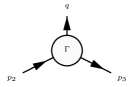
Figure 1: Kinematics used for the correlators of fermion bilinears.

Vertex functions are defined as:

$$G^{a}_{\Gamma}(p_{3},p_{2})=\langle O^{a}_{\Gamma}(q)\bar{\psi}(p_{3})\psi(p_{2})\rangle\,,$$ (3)

i.e. as the correlator of two fermions together with the fermion bilinear operator $O^{a}_{\Gamma}=\bar{\psi}\Gamma\tau^{a}\psi$, which is a flavor non-singlet with $\tau^{a}$ denoting a generic generator of rotations in flavor space. $\Gamma$ spans all the elements of the basis of the Clifford algebra, which we denote as $\Gamma=\mathrm{S},\mathrm{P},\mathrm{V},\mathrm{A},\mathrm{T}$. We consider a fermion doublet which is degenerate in mass, $m_{1}=m_{2}=m$, and take $\tau^{a}=\frac{\sigma^{+}}{2}=\frac{1}{2}(\sigma^{1}+i\sigma^{2})$ giving $O_{\Gamma}=\overline{\psi}_{1}\Gamma{\psi_{2}}$. The amputated vertex function is

$$\Lambda^{a}_{\Gamma}(p_{2},p_{3})=S(p_{3})^{-1}G^{a}_{\Gamma}(p_{3},p_{2})S(p_{2})^{-1}\,,$$ (4)

where $S(p)$ is the fermion propagator:

$$S(p)=\frac{i}{\not{\hbox{\kern-2.0pt$p$}}-m-\Sigma(p)+i\epsilon}\,.$$ (5)

Note that for each leg being amputated, the fermion propagator with the corresponding flavor needs to be used.

Let us consider chiral symmetry transformations with a regulator that does not break the symmetry, like e.g. dimensional regularization. The infinitesimal vector and axial non-singlet SU(2) transformations change $\bar{\psi}$ and $\psi$ in the path integral, yielding the bare vector and axial WIs. Written in terms of $\Lambda^{a}_{\mathrm{V}}$ and $\Lambda^{a}_{\mathrm{A}}$ they are

$$q\cdot\Lambda^{a}_{\mathrm{V}} =iS(p_{2})^{-1}-iS(p_{3})^{-1}\,,$$ (6)

$$q\cdot\Lambda^{a}_{\mathrm{A}} =2mi\Lambda^{a}_{\mathrm{P}}-\gamma_{5}iS(p_{2})^{-1}-iS(p_{3})^{-1}\gamma_{5}\,.$$ (7)

The renormalized quantities are defined as follows:

$$\psi_{R}=Z_{q}^{1/2}\psi\,,\quad m_{qR}=Z_{m_{q}}m_{q}\,,\quad O_{\Gamma,R}=Z_{\Gamma}O_{\Gamma}\,,$$ (8)

yielding the renormalized propagator and amputated vertex functions

$$S_{R}(p)=Z_{q}S(p)\,,\quad\Lambda_{\Gamma,R}(p_{2},p_{3})=\frac{Z_{\Gamma}}{Z_{q}}\Lambda_{\Gamma}(p_{2},p_{3})\,,$$ (9)

where $q=l,H$ for light and heavy quarks respectively. Note that for each leg being amputated, the fermion propagator with the corresponding flavor needs to be used. In the rest of this section, we will denote $m_{l}$ by $m$ and ${m_{H}}$ by $M$ and suppress the flavor index $a$ to keep the notation simple.

The mSMOM renormalization condition are defined away from the chiral limit, at some reference mass $\bar{m}$ which can be chosen freely:

$$\lim_{M_{R}\to\overline{m}} \left.\frac{1}{12p^{2}}\mbox{Tr}\left[iS_{R}(p)^{-1}\not{\hbox{\kern-2.0pt$p$}}\right]\right|_{p^{2}=-\mu^{2}}=1\,,$$ (10)

$$\lim_{M_{R}\to\overline{m}} \frac{1}{12M_{R}}\left\{\left.\mbox{Tr}\left[-iS_{R}(p)^{-1}\right]\right|_{p^{2}=-\mu^{2}}-\frac{1}{2}\left.\mbox{Tr}\left[\left(q\cdot\Lambda_{\mathrm{A},R}\right)\gamma_{5}\right]\right|_{\mathrm{sym}}\right\}=1\,,$$ (11)

$$\lim_{M_{R}\to\overline{m}} \frac{1}{12q^{2}}\mbox{Tr}\left.\left[\left(q\cdot\Lambda_{\mathrm{V},R}\right)\not{\hbox{\kern-2.0pt$q$}}\right]\right|_{\mathrm{sym}}=1\,,$$ (12)

$$\lim_{M_{R}\to\overline{m}} \frac{1}{12q^{2}}\mbox{Tr}\left.\left[\left(q\cdot\Lambda_{\mathrm{A},R}-2M_{R}i\Lambda_{\mathrm{P},R}\right)\gamma_{5}\not{\hbox{\kern-2.0pt$q$}}\right]\right|_{\mathrm{sym}}=1\,,$$ (13)

$$\lim_{M_{R}\to\overline{m}} \frac{1}{12i}\mbox{Tr}\left.\left[\Lambda_{\mathrm{P},R}\gamma_{5}\right]\right|_{\mathrm{sym}}=1\,,$$ (14)

$$\lim_{M_{R}\to\overline{m}} \Bigg{\{}\frac{1}{12}\text{Tr}\left[\Lambda_{S,R}\right]-\frac{1}{6q^{2}}\text{Tr}\left[2iM_{R}\Lambda_{P,R}\gamma_{5}\not{q}\right]\Bigg{\}}\Bigg{|}_{\text{sym}}=1\,.$$ (15)

As compared to the SMOM scheme [2], only the renormalization conditions for the axial and the scalar vertex functions are modified, with the modifications being proportional to the mass, and vanishing at tree-level. Therefore, in the chiral limit $\bar{m}\to 0$, these conditions reduce to SMOM exactly. Similar to SMOM, the conditions for mSMOM are spelled out in such a way to preserve the renormalized WIs and give $Z_{V}=Z_{A}=1$. The non-perturbative derivation follows similar steps to those taken in [2]. For $Z_{V}$, using the relation between renormalized and bare vertex functions, and Eq. (12), we obtain

$$\lim_{M_{R}\to\overline{m}}\frac{1}{12q^{2}} \mbox{Tr}\left.\left[\left(q\cdot\Lambda_{\mathrm{V}}\right)\not{\hbox{\kern-2.0pt$q$}}\right]\right|_{\mathrm{sym}}=\lim_{M_{R}\to\overline{m}}\frac{Z_{q}}{Z_{\mathrm{V}}}\frac{1}{12q^{2}}\mbox{Tr}\left.\left[\left(q\cdot\Lambda_{\mathrm{V},R}\right)\not{\hbox{\kern-2.0pt$q$}}\right]\right|_{\mathrm{sym}}$$ (16)

$$=\frac{Z_{q}}{Z_{\mathrm{V}}}\,.$$ (17)

Using the vector Ward identity, Eq. (6), the LHS of the expression above can be written as

$$\lim_{M_{R}\to\overline{m}}\frac{1}{12q^{2}} \mbox{Tr}\left.\left[\left(iS(p_{2})^{-1}-iS(p_{3})^{-1}\right)\not{\hbox{\kern-2.0pt$q$}}\right]\right|_{\mathrm{sym}}=\frac{1}{12q^{2}}\mbox{Tr}\left.\left[iS(q)^{-1}\not{\hbox{\kern-2.0pt$q$}}\right]\right|_{\mathrm{sym}}$$ (18)

$$=Z_{q}\lim_{M_{R}\to\overline{m}}\frac{1}{12q^{2}}\mbox{Tr}\left.\left[iS_{R}(q)^{-1}\not{\hbox{\kern-2.0pt$q$}}\right]\right|_{q^{2}=-\mu^{2}}=Z_{q}\,.$$ (19)

Comparing Eqs. (17) and (19) yields $Z_{\mathrm{V}}=1$.

Because of the modified renormalization condition for the renormalization of the axial vertex function, the computation of $Z_{\mathrm{A}}$ and $Z_{M}Z_{\mathrm{P}}$ are coupled in the mSMOM scheme. The axial Ward identity, Eq. (7), can be rewritten in terms of renormalized quantities:

$$\frac{1}{Z_{\mathrm{A}}}q\cdot\Lambda_{\mathrm{A},R} -\frac{1}{Z_{M}Z_{\mathrm{P}}}2M_{R}i\Lambda_{\mathrm{P},R}=-\left\{\gamma_{5}iS_{R}(p_{2})^{-1}+iS_{R}(p_{3})^{-1}\gamma_{5}\right\}\,.$$ (20)

Two independent equations can be obtained by multipling Eq. (20) by $\gamma^{5}\not{\hbox{\kern-2.0pt$q$}}$ and $\gamma_{5}$ respectively, taking the trace, and evaluating correlators at the symmetric point. In the first case we obtain

$$(Z_{\mathrm{A}}-1)=\left(1-\frac{Z_{\mathrm{A}}}{Z_{M}Z_{\mathrm{P}}}\right)C_{mP}\,,$$ (21)

where

$$C_{m\mathrm{P}}=\lim_{M_{R}\to\overline{m}}\frac{1}{12q^{2}}\mbox{Tr}\left.\left[2iM_{R}\Lambda_{\mathrm{P},R}\gamma_{5}\not{\hbox{\kern-2.0pt$q$}}\right]\right|_{\mathrm{sym}}\,.$$ (22)

The second equation instead yields

$$(Z_{\mathrm{A}}-1)C_{qA}=-2Z_{\mathrm{A}}\left(1-\frac{1}{Z_{M}Z_{\mathrm{P}}}\right)\,,$$ (23)

where we have introduced one more constant

$$Z_{\mathrm{P}}C_{q\mathrm{A}}=\lim_{M_{R}\to\overline{m}}\frac{1}{12M_{R}}\mbox{Tr}\left.\left[q\cdot\Lambda_{\mathrm{A},R}\gamma_{5}\right]\right|_{\mathrm{sym}}\,.$$ (24)

It is easy to verify that $Z_{\mathrm{A}}=1$, $Z_{M}Z_{\mathrm{P}}=1$ is the unique solution of the system. It can be readily observed that given these condition Eq. (20) gives the correct renormalized axial WI. In particular $Z_{V}$ and $Z_{A}$ are independent of the renormalization scale $\mu$.

3 Perturbative computation

We have checked all the above properties of the mSMOM scheme by performing an explicit one-loop computation in perturbation theory using dimensional regularization, keeping explicitly the dependence on the bare mass $m$. We start from the 1-loop expression

$$\Lambda^{(1)}_{\Gamma}(p_{2},p_{3})=-ig^{2}C_{2}(F)\int_{k}\frac{\gamma_{\alpha}\left[\not{\hbox{\kern-2.0pt$p$}}_{3}-\not{\hbox{\kern-2.0pt$k$}}+m\right]\Gamma\left[\not{\hbox{\kern-2.0pt$p$}}_{2}-\not{\hbox{\kern-2.0pt$k$}}+m\right]\gamma^{\alpha}}{k^{2}\left[\left(p_{3}-k\right)^{2}-m^{2}\right]\left[\left(p_{2}-k\right)^{2}-m^{2}\right]}\,,$$ (25)

and rewrite the numerator in terms of scalar coefficients [9, 10] multiplying some form factors, depending on which vertex is being considered. The scalar coefficients are functions of $m^{2}/\mu^{2}$. Computing the vertex for all $\Gamma=S,P,V,A$ and the quark propagator at one loop, we check that the results satisfy the bare WIs and reproduce the results in Ref.[2] as $m\to 0$. We then use the renormalization conditions Eq. 10-15, and obtain $Z_{\mathrm{V}}=Z_{\mathrm{A}}=1$, $Z_{\mathrm{P}}=Z_{\mathrm{S}}$, $Z_{m}Z_{\mathrm{P}}=1$.

The details of this calculation goes beyond the scope of these proceedings, and will be reported in details in a forthcoming publication.

4 Mass non-degenerate scheme

We will now consider the renormalization scheme for the case of non-singlet, mass non-degenerate vertex functions with the mass matrix taking the form

$$\mathcal{M}=\begin{pmatrix}M&0\\ 0&m\end{pmatrix},$$ (26)

where $M$ and $m$ are masses of the heavy and the light quarks respectively. In what follows we will be interested in fermion bilinears of the form $O^{+}=\overline{H}\Gamma l$ by choosing the flavor rotation matrix to be $\tau^{a}=\tau^{+}=\frac{\sigma^{+}}{2}=\frac{1}{2}(\sigma^{1}+i\sigma^{2})$. For clarity, we will leave the flavor index $``+"$ explicit in the WIs, but will suppress it for the rest of the section to keep the notation simple. The curly letters ($\mathcal{V},\mathcal{A},\mathcal{P},\mathcal{S}$) denote the heavy-light bilinears. The vector and axial Ward identities are as follows:

$$q\cdot\Lambda^{+}_{\mathcal{V}}=(M-m)\Lambda^{+}_{\mathcal{S}}+iS_{H}(p_{2})^{-1}-iS_{l}(p_{3})^{-1}\,,$$ (27)

$$q\cdot\Lambda^{+}_{\mathcal{A}}=(M+m)i\Lambda^{+}_{\mathcal{P}}-\gamma_{5}iS_{H}(p_{2})^{-1}-iS_{l}(p_{3})^{-1}\gamma_{5}\,.$$ (28)

4.1 Modified renormalization conditions

The mSMOM scheme for the heavy-light mixed case is defined by imposing the following set of conditions at some reference mass $\overline{m}$:

$$\lim_{\begin{subarray}{c}m_{R}\to 0\\ M_{R}\to\overline{m}\end{subarray}} \frac{1}{12q^{2}}\mbox{Tr}\left.\left[\left(q\cdot\Lambda_{\mathcal{V},R}-(M_{R}-m_{R})\Lambda_{\mathcal{S},R}\right)\not{\hbox{\kern-2.0pt$q$}}\right]\right|_{\mathrm{sym}}=\lim_{\begin{subarray}{c}m_{R}\to 0\\ M_{R}\to\overline{m}\end{subarray}}\frac{1}{12q^{2}}\mbox{Tr}\left[\left(i\zeta^{-1}S_{H,R}(p_{2})^{-1}-i\zeta S_{l,R}(p_{3})^{-1}\right)\not{\hbox{\kern-2.0pt$q$}}\right]\,,$$ (29)

$$\lim_{\begin{subarray}{c}m_{R}\to 0\\ M_{R}\to\overline{m}\end{subarray}} \frac{1}{12q^{2}}\mbox{Tr}\left.\left[\left(q\cdot\Lambda_{\mathcal{A},R}-(M_{R}+m_{R})i\Lambda_{\mathcal{P},R}\right)\gamma_{5}\not{\hbox{\kern-2.0pt$q$}}\right]\right|_{\mathrm{sym}}=\lim_{\begin{subarray}{c}m_{R}\to 0\\ M_{R}\to\overline{m}\end{subarray}}\frac{1}{12q^{2}}\mbox{Tr}\left[\left(-i\gamma^{5}\zeta^{-1}S_{H,R}(p_{2})^{-1}-i\zeta S_{l,R}(p_{3})^{-1}\gamma^{5}\right)\gamma_{5}\not{\hbox{\kern-2.0pt$q$}}\right]\,,$$ (30)

$$\lim_{\begin{subarray}{c}m_{R}\to 0\\ M_{R}\to\overline{m}\end{subarray}} \frac{1}{12i}\mbox{Tr}\left.\left[\Lambda_{\mathcal{P},R}\gamma_{5}\right]\right|_{\mathrm{sym}}=\lim_{\begin{subarray}{c}m_{R}\to 0\\ M_{R}\to\overline{m}\end{subarray}}\Bigg{\{}\frac{1}{12(M_{R}+m_{R})}\left\{\left.\mbox{Tr}\left[-i\zeta^{-1}S_{H,R}(p)^{-1}\right]\right|_{p^{2}=-\mu^{2}}-\frac{1}{2}\left.\mbox{Tr}\left[\left(q\cdot\Lambda_{\mathcal{A},R}\right)\gamma_{5}\right]\right|_{\mathrm{sym}}\right\}+$$

$$\ \ \ \ \ \ \ \ \ \ \ \ \ \ \ \ \ \ \ \ \ \ \ \ \ \ \ \ \ \ \ \ \ \ \ \ \ \ \ \ \frac{1}{12(M_{R}+m_{R})}\left\{\left.\mbox{Tr}\left[-i\zeta S_{l,R}(p)^{-1}\right]\right|_{p^{2}=-\mu^{2}}-\frac{1}{2}\left.\mbox{Tr}\left[\left(q\cdot\Lambda_{\mathcal{A},R}\right)\gamma_{5}\right]\right|_{\mathrm{sym}}\right\}\Bigg{\}}\,.$$ (31)

where $\zeta$ denotes the ratio of the light to the heavy field renormalizations, i.e. $\zeta=\frac{\sqrt{Z_{l}}}{\sqrt{Z_{H}}}$. In the degenerate mass limit $\zeta\to 1$ and the mixed mSMOM prescription reduces to the mSMOM and SMOM ones. The curly subscripts denote heavy-light mixed vertices. The renormalization conditions for $Z_{l},\ Z_{H}$ and $Z_{m}$ remain unaltered as they are independently determined from the corresponding degenerate, massive and massless schemes of the previous sections. As usual the renormalization conditions are satisfied by the tree level values of the field correlators.

4.2 Renormalization constants

The renormalization constants in this scheme are obtained once again from the WIs. We multiply the vector WI Eq. 27 by $\not{\hbox{\kern-2.0pt$q$}}$, take the trace and write the bare quantities in terms of the renormalized ones. Using Eq. 29 we obtain the solution $Z_{\mathcal{V}}=1$ and

$$Z_{\mathcal{S}}=\frac{\frac{M_{R}}{Z_{M}}-\frac{m_{R}}{Z_{m}}}{M_{R}-m_{R}}\,.$$ (32)

For the axial current we follow a similar procedure, starting from the bare mixed axial WI Eq. 28. Multiplying by $\gamma^{5}\not{\hbox{\kern-2.0pt$q$}}$ and $\gamma_{5}$ respectively and taking the trace gives two independent equations. In the first case we use Eq. 30 which gives $Z_{\mathcal{A}}=1$ and

$$Z_{\mathcal{P}}=\frac{\frac{M_{R}}{Z_{M}Z_{\mathcal{P}}}+\frac{m_{R}}{Z_{m}Z_{\mathcal{P}}}}{M_{R}+m_{R}}\,,$$ (33)

as a solution. Note that in the degenerate mass limit, we recover $Z_{m}Z_{\mathrm{P}}=1$. In the second case, we take the trace with $\gamma^{5}$ and make use of Eq. 4.1, to obtain the solutions $Z_{\mathcal{A}}=1$ and $Z_{\mathcal{P}}$ as in Eq. 33. One can easily check that this solution is unique.

5 Lattice regularization

If we use lattice as a regulator, the axial WI takes the form

$$\nabla^{*}_{\mu}\langle A^{a}_{\mu}(x)\psi(y)\bar{\psi}(z)\rangle=2m \langle P^{a}(x)\psi(y)\bar{\psi}(z)\rangle+\mathrm{contact\ terms}$$

$$+\langle X^{a}(x)\psi(y)\bar{\psi}(z)\rangle\,.$$ (34)

where $X^{a}(x)$ is the explicit chiral symmetry breaking term due to the lattice regulator. Since translational invariance of the action is recovered in the naive $a\to 0$ limit, the contribution from the explicit breaking by the regulator is given by by higher-dimensional operators $X^{a}(x)=aO^{a}_{5}(x)$, where the suffix 5 indicates the fact that these operators have classical dimension greater or equal to 5. In order to discuss the continuum limit of Eq. 5, each term needs to be renormalized. In particular the higher dimensional operator $O^{a}_{5}(x)$ mixes with the lower dimensional ones appearing in Eq. 5:

$$O^{a}_{5R}(x)=Z_{5}\left[O^{a}_{5}(x)+\frac{\overline{m}}{a}P^{a}(x)+\frac{Z_{\mathrm{A}}-1}{a}\nabla^{*}_{\mu}A^{a}_{\mu}(x)\right]\,.$$ (35)

According to Ref. [3] the power divergences due to this mixing do not contribute to the anomalous dimensions, i.e. they do not depend on the renormalization scale $\mu$ to all orders of perturbation theory,

$$A^{a}_{R,\mu}=Z_{\mathrm{A}}\left(g,am\right)A^{a}_{\mu}\,,$$ (36)

and the renormalized current satisfies the Ward identities up to terms of order $a$. It is important to notice that the dependence of $Z_{A}$ on the mass is a lattice artefact.

6 Conclusion

We have developed a massive renormalization scheme, mSMOM, for non-singlet fermion bilinear operators in QCD with non-exceptional momenta away from the chiral limit. The renormalization conditions are imposed at some value $\bar{m}$ of the renormalized mass. In the limit where $\bar{m}\to 0$, our scheme reduces to the familiar SMOM scheme [2].

We have shown that the renormalized WIs for the case of both degenerate and non-degenerate masses are satisfied non-perturbatively, giving $Z_{V}=1$ and $Z_{A}=1$ for conserved currents. In order to gain a better understanding of the properties of the mSMOM scheme we have performed an explicit one-loop computation in perturbations theory using dimensional regularization. Often on the lattice, we obtain local currents that have to be renormalized. In this case the renormalization constants can be obtained by taking ratios of vertex functions with an appropriate projector and using both SMOM and mSMOM conditions to extract $Z_{V}^{\text{local}}$ and $Z_{A}^{\text{local}}$. The details of this procedure are deferred to a forthcoming publication.

- [1] G. Martinelli, C. Pittori, C. T. Sachrajda, M. Testa and A. Vladikas, Nucl. Phys. B 445 (1995) 81 doi:10.1016/0550-3213(95)00126-D [hep-lat/9411010].
- [2] C. Sturm et al., Phys. Rev . D 80 (2009) 014501 doi:10.1103/PhysRevD.80.014501 [hep-ph/0901.2599].
- [3] M. Testa, JHEP 9804 (1998) 002 doi:10.1088/1126-6708/1998/04/002 [hep-th/9803147].
- [4] T. Blum et al., Phys. Rev. D 66 (2002) 014504 doi:10.1103/PhysRevD.66.014504 [hep-lat/0102005].
- [5] A. Vladikas, Modern perspectives in lattice QCD, Les Houches International School (2009), [hep-lat/1103.1323].
- [6] W. E. Caswell, A. D. Kennedy, Phys. Rev . D 25 (1982) 392, doi:10.1103/PhysRevD.25.392,
- [7] S. Weinberg, Phys. Rev . D 8 (1973) 3497-3509, doi:10.1103/PhysRevD.8.3497,
- [8] V. A. Smirnov, Feynman integral calculus (2006).
- [9] F. Chavez, C. Duhr, JHEP 11 (2012), doi: 10.1007/JHEP11(2012)114, [hep-ph/1209.2722].
- [10] A. V. Smirnov, Fire5 Mathematica Package, Algorithm FIRE – Feynman Integral REduction, JHEP 10 (2008), doi: 10.1088/1126-6708/2008/10/107, [hep-ph/0807.3243].