UFIFT-QG-16-05

Determining Cosmology for a Nonlocal Realization of MOND

M. Kim¹, M. H. Rahat², M. Sayeb³, L. Tan⁴, R. P. Woodard⁵ and B. Xu⁶

Department of Physics, University of Florida,
Gainesville, FL 32611, UNITED STATES

ABSTRACT

We numerically determine the cosmological branch of the free function in a nonlocal metric-based modification of gravity which provides a relativistic generalization of Milgrom’s Modified Newtonian Dynamics. We are able to reproduce the $\Lambda$CDM expansion history over virtually all of cosmic history, including the era of radiation domination during Big Bang Nucleosynthesis, the era of matter domination during Recombination, and most of the era of vacuum energy domination. The very late period of $0\leq z\mathrel{\raise 1.29167pt\hbox{$<$\kern-7.5pt\lower 4.30554pt\hbox{$\sim$}}}0.0880$, during which the model deviates from the $\Lambda$CDM expansion history, is interesting because it causes the current value of the Hubble parameter to be about 4.5% larger than it would be for the $\Lambda$CDM model. This may resolve the tension between inferences of $H_{0}$ which are based on data from large redshift and inferences based on Hubble plots.

PACS numbers: 04.50.Kd, 95.35.+d, 98.62.-g

¹ pq8556@ufl.edu ⁴ billy@ufl.edu
² mrahat@ufl.edu ⁵ woodard@phys.ufl.edu
³ sayebms1@ufl.edu ⁶ binxu@ufl.edu

1 Introduction

There have been impressive confirmations of general relativity in the solar system and from binary pulsars [1]. Most recently the existence of gravitational radiation has been established [2]. However, general relativity does not do such a good job at explaining certain observed regularities of rotationally supported galaxies:

• The Baryonic Tully-Fisher Relation ($v^{4}_{\infty}=a_{0}GM$) between the asymptotic rotational speed $v_{\infty}$ and the total mass $M$ in baryons, where $a_{0}\approx 1.2\times 10^{-10}~{}{\rm m/s}^{2}$ [3];

• Milgrom’s Law that non-baryonic dark matter is required when the gravitational acceleration from baryonic matter falls below $a_{0}$ [4];

• Freeman’s Law ($\Sigma<\frac{a_{0}}{G}$) for the surface density $\Sigma$ [5]; and

• Sancisi’s Law that features in the rotation curve are correlated with features in the surface brightness [6].

Analogous regularities have been observed for pressure-supported galaxies [7]. These laws may signal undiscovered features in the way general relativity combines baryons with much more massive pools of dark matter to form cosmic structures. However, it is disconcerting that increasingly sensitive experiments have so far failed to detect all this dark matter [8, 9, 10].

In the absence of laboratory detection of dark matter it is worth while examining the possibility that gravity is modified instead. Milgrom has proposed a particularly promising modification for what would be the static, weak field limit of such a theory [11, 12, 13]. There is no question that Milgrom’s MOdified Newtonian Dynamics (MOND) explains the various observed regularities of galactic structure [14, 15]. The challenge is to extend MOND to a fully relativistic theory that can be used to study the same range of phenomena as general relativity. Two approaches have been followed:

• Models in which other fields carry the MOND force [16, 17]; and

• Models in which an algebraic function of a nonlocal invariant of the metric is added to the Lagrangian — $R\longrightarrow R+\frac{a_{0}^{2}}{c^{4}}f_{y}(Z[g])$ — [18].

The purpose of this paper is to specify $f_{y}(Z)$ for the latter approach.

The modified gravity equations have been derived for a general metric $g_{\mu\nu}$ and a general function $f_{y}(Z)$ [19, 20]. A crucially important point is that whereas the nonlocal invariant $Z[g]$ is positive for gravitationally bound systems, it is typically negative for cosmological systems in which time dependence is more significant than spatial dependence. Explaining the regularities of galaxies fixes the algebraic function for positive arguments [18],

$$f_{y}(Z)=\frac{1}{2}Z-\frac{1}{6}Z^{\frac{3}{2}}+O(Z^{2})\;.$$ (1)

Preserving solar system tests (and those at strong fields) requires that the function fall off for large, positive $Z$. For example, the following simple form would suffice [18],

$$Z>0\qquad\Longrightarrow\qquad f_{y}(Z)=\frac{1}{2}Z\exp\Bigl{[}-\frac{1}{3}\sqrt{Z}\,\Bigr{]}\;.$$ (2)

But how the function depends on negative $Z$ must be regarded as a free parameter at this stage.

The purpose of this paper is to show that the function $f_{y}(Z)$ can be chosen so as to reproduce the $\Lambda$CDM expansion history — which is itself just a model, with free parameters — over almost the full range of cosmic evolution. It turns out that the nonlocal invariant $Z$ fails to be monotonic at very late times, which means that our nonlocal realization of MOND inevitably deviates from $\Lambda$CDM cosmology. However, this deviation is serendipitous because it makes the current value of the Hubble parameter about 4.5% larger, which has the potential to explain why high redishift determinations of $H_{0}$ give a smaller value than low redshift determinations.

In section 2 we review the model, defining the nonlocal invariant $Z[g]$ and specializing the field equations to a general, spatially flat cosmology. Section 3 assumes the $\Lambda$CDM expansion history and uses this to derive the form of $f_{y}(Z)$ must take for large negative $Z$ and for small negative $Z$. Section 4 presents a numerical solution of the full problem, which includes the failure of $Z$ to be monotonic at very late times and the resulting deviation from $\Lambda$CDM cosmology. What all this means is discussed in section 5.

2 The Model

The purpose of this section is to briefly review the nonlocal metric realization of MOND [18, 19]. We begin by defining the full invariant $Z[g](x)$, then give the general field equations. The section closes by specializing $Z[g](x)$ and the field equations to the homogeneous and isotropic geometry of cosmology.

The gravitational Lagrangian takes the form,

$$\mathcal{L}=\frac{c^{4}}{16\pi G}\Biggl{\{}R+\frac{a^{2}_{0}}{c^{4}}f_{y}\Bigl{(}Z[g]\Bigr{)}\Biggr{\}}\sqrt{-g}\;.$$ (3)

The dimensionless nonlocal invariant $Z[g]$,

$$Z[g]\equiv\frac{4c^{4}}{a_{0}^{2}}\,g^{\mu\nu}\Bigl{[}\partial_{\mu}\frac{1}{\kern 1.0pt\vbox{\hrule height=1.2pt\hbox{\vrule width=1.2pt\hskip 3.0pt\vbox{\vskip 6.0pt}\hskip 3.0pt\vrule width=0.6pt}\hrule height=0.6pt}\kern 1.0pt}R_{\alpha\beta}u^{\alpha}u^{\beta}\Bigr{]}\Bigl{[}\partial_{\nu}\frac{1}{\kern 1.0pt\vbox{\hrule height=1.2pt\hbox{\vrule width=1.2pt\hskip 3.0pt\vbox{\vskip 6.0pt}\hskip 3.0pt\vrule width=0.6pt}\hrule height=0.6pt}\kern 1.0pt}R_{\rho\sigma}u^{\rho}u^{\sigma}\Bigr{]}\;,$$ (4)

is constructed using three geometrical quantities:

1. The inverse scalar d’Alembertian,

   $$\kern 1.0pt\vbox{\hrule height=1.2pt\hbox{\vrule width=1.2pt\hskip 3.0pt\vbox{\vskip 6.0pt}\hskip 3.0pt\vrule width=0.6pt}\hrule height=0.6pt}\kern 1.0pt\equiv\frac{1}{\sqrt{-g}}\,\partial_{\mu}\Bigl{(}\sqrt{-g}\,g^{\mu\nu}\partial_{\nu}\Bigr{)}\;,$$ (5)

   where the inverse is defined using retarded boundary conditions.

2. A normalized timelike 4-velocity $u^{\mu}[g](x)$,

   $$\chi[g](x)\equiv-\frac{1}{\kern 1.0pt\vbox{\hrule height=1.2pt\hbox{\vrule width=1.2pt\hskip 3.0pt\vbox{\vskip 6.0pt}\hskip 3.0pt\vrule width=0.6pt}\hrule height=0.6pt}\kern 1.0pt}\,1\qquad\Longrightarrow\qquad u^{\mu}[g]\equiv\frac{-g^{\mu\nu}\partial_{\nu}\chi[g]}{\sqrt{-g^{\alpha\beta}\partial_{\alpha}\chi[g]\partial_{\beta}\chi[g]}}\;.$$ (6)

3. The Ricci tensor $R_{\mu\nu}$.

At this point a digression is in order to comment on the probable genesis of nonlocality. We believe that fundamental theory is local, but the nonlocal Lagrangian (3) represents the gravitational vacuum polarization of the vast ensemble of infrared gravitons created by primordial inflation. These gravitons were not present at the beginning of inflation, and their wave lengths do not extend to arbitrarily small scales. This in no way changes the purely phenomenological status of the nonlocal model (3), but it does explain two of the model’s features which would otherwise seem absurd [20]:

• That there is an initial time at which to specify the initial conditions of the inverse d’Alembertian; and

• That MOND corrections affect large scales but not small scales.

The simplest way to present the general field equations is by introducing nondynamical, auxiliary scalars after the method of Nojiri and Odintsov [22]. Localizing the Lagrangian (3) requires four such scalars [19],

$$\mathcal{L}=\frac{c^{4}}{16\pi G}\Biggl{\{}R+\frac{a_{0}^{2}}{c^{4}}f_{y}\Bigl{(}\frac{g^{\mu\nu}\partial_{\mu}\phi\partial_{\nu}\phi}{c^{-4}a_{0}^{2}}\Bigr{)}$$ (7)

$$\hskip 56.9055pt-\Bigl{[}\partial_{\mu}\xi\partial_{\nu}\phi g^{\mu\nu}\!+\!2\xi R_{\mu\nu}u^{\mu}u^{\nu}\Bigr{]}-\Bigl{[}\partial_{\mu}\psi\partial_{\nu}\chi g^{\mu\nu}\!-\!\psi\Bigr{]}\Biggr{\}}\sqrt{-g}\;,\qquad$$

where $D_{\mu}$ denotes the covariant derivative operator and $u^{\mu}[g]$ is defined in terms of the scalar $\chi$ according to the right hand side of (6). The auxiliary scalars must not be considered as independent degrees of freedom because two of them would be ghosts [23, 24]. The four scalars are rather nonlocal functionals of the metric defined by solving their equations of motion with retarded boundary conditions ,

$$\phi[g]=\frac{2}{\kern 1.0pt\vbox{\hrule height=1.2pt\hbox{\vrule width=1.2pt\hskip 3.0pt\vbox{\vskip 6.0pt}\hskip 3.0pt\vrule width=0.6pt}\hrule height=0.6pt}\kern 1.0pt}R_{\alpha\beta}u^{\alpha}u^{\beta} \!\!,\!\! \chi[g]=-\frac{1}{\kern 1.0pt\vbox{\hrule height=1.2pt\hbox{\vrule width=1.2pt\hskip 3.0pt\vbox{\vskip 6.0pt}\hskip 3.0pt\vrule width=0.6pt}\hrule height=0.6pt}\kern 1.0pt}1\;,$$ (8)

$$\xi[g]=\frac{2}{\kern 1.0pt\vbox{\hrule height=1.2pt\hbox{\vrule width=1.2pt\hskip 3.0pt\vbox{\vskip 6.0pt}\hskip 3.0pt\vrule width=0.6pt}\hrule height=0.6pt}\kern 1.0pt}D^{\mu}\Biggl{[}\partial_{\mu}\phi f^{\prime}_{y}\Bigl{(}\frac{g^{\rho\sigma}\partial_{\rho}\phi\partial_{\sigma}\phi}{c^{-4}a_{0}^{2}}\Bigr{)}\Biggr{]} \!\!,\!\! \psi[g]=\frac{4}{\kern 1.0pt\vbox{\hrule height=1.2pt\hbox{\vrule width=1.2pt\hskip 3.0pt\vbox{\vskip 6.0pt}\hskip 3.0pt\vrule width=0.6pt}\hrule height=0.6pt}\kern 1.0pt}D_{\mu}\Biggl{[}\frac{\xi(g^{\mu\rho}\!+\!u^{\mu}u^{\rho})u^{\sigma}R_{\rho\sigma}}{\sqrt{-g^{\alpha\beta}\partial_{\alpha}\chi\partial_{\beta}\chi}}\Biggr{]}.\quad$$ (9)

The modified gravitational field equations are [19],

$$R_{\mu\nu}+\frac{1}{2}g_{\mu\nu}\Bigl{[}-R-\frac{a_{0}^{2}}{c^{4}}f_{y}+g^{\rho\sigma}\Bigl{(}\partial_{\rho}\xi\partial_{\sigma}\phi\!+\!\partial_{\rho}\psi\partial_{\sigma}\chi\Bigr{)}+2\xi u^{\rho}u^{\sigma}R_{\rho\sigma}-\psi\Bigr{]}$$ (10)

$$+\partial_{\mu}\phi\partial_{\nu}\phi f_{y}^{\prime}-\partial_{(\mu}\xi\partial_{\nu)}\phi-\partial_{(\mu}\psi\partial_{\nu)}\chi-2\xi\Bigl{[}2u_{(\mu}u^{\alpha}R_{\nu)\alpha}\!+\!u_{\mu}u_{\nu}u^{\alpha}u^{\beta}R_{\alpha\beta}\Bigr{]}$$

$$\hskip 8.5359pt-\Bigl{[}\kern 1.0pt\vbox{\hrule height=1.2pt\hbox{\vrule width=1.2pt\hskip 3.0pt\vbox{\vskip 6.0pt}\hskip 3.0pt\vrule width=0.6pt}\hrule height=0.6pt}\kern 1.0pt(\xi u_{\mu}u_{\nu})+g_{\mu\nu}D_{\alpha}D_{\beta}(\xi u^{\alpha}u^{\beta})-2D_{\alpha}D_{(\mu}(\xi u_{\nu)}u^{\alpha})\Bigr{]}=\frac{8\pi G}{c^{4}}\,T_{\mu\nu}\;.\qquad$$

It remains to specialize relations (8-10) to the homogeneous, isotropic and spatially flat geometry relevant to cosmology,

$$g_{\mu\nu}dx^{\mu}dx^{\nu}=-c^{2}dt^{2}+a^{2}(t)d\vec{x}\cdot d\vec{x}\quad\Longrightarrow\quad H(t)\equiv\frac{\dot{a}}{a}\quad,\quad\epsilon(t)\equiv-\frac{\dot{H}}{H^{2}}\;.$$ (11)

In this geometry the auxiliary scalars become [19],

$$\phi(t) = -6\!\!\int_{t_{i}}^{t}\!\!\frac{dt^{\prime}}{a^{3}(t^{\prime})}\!\!\int_{t_{i}}^{t^{\prime}}\!\!dt^{\prime\prime}a^{3}(t^{\prime\prime})H^{2}(t^{\prime\prime})\Bigl{[}\epsilon(t^{\prime\prime})\!-\!1\Bigr{]}\;\Longrightarrow\;Z(t)=-\frac{\dot{\phi}^{2}(t)}{c^{-2}a_{0}^{2}}\;,\qquad$$ (12)

$$\chi(t) = \!\!\int_{t_{i}}^{t}\!\!\frac{dt^{\prime}}{a^{3}(t^{\prime})}\!\!\int_{t_{i}}^{t^{\prime}}\!\!dt^{\prime\prime}a^{3}(t^{\prime\prime})\qquad\Longrightarrow\qquad u^{\mu}(t)=\delta^{\mu}_{0}\;,\qquad$$ (13)

$$\xi(t) = 2\!\!\int_{t_{i}}^{t}\!\!dt^{\prime}\dot{\phi}(t^{\prime})f_{y}^{\prime}\Bigl{(}Z(t^{\prime})\Bigr{)}\qquad,\qquad\psi(t)=0\;,$$ (14)

where $t_{i}$ is the initial time. The gravitational field equations are [19],

$$3H^{2}\!+\!\frac{a_{0}^{2}}{2c^{2}}f_{y}(Z)\!+\!3H\dot{\xi}\!+\!6H^{2}\xi = \frac{8\pi G}{c^{2}}\,\rho\;,$$ (15)

$$-2\dot{H}\!-\!3H^{2}\!-\!\frac{a_{0}^{2}}{2c^{2}}\,f_{y}(Z)\!-\!\ddot{\xi}\!-\!\Bigl{(}\frac{\dot{\phi}}{2}\!+\!4H\Bigr{)}\dot{\xi}\!-\!\Bigl{(}4\dot{H}\!+\!6H^{2}\Bigr{)}\xi = \frac{8\pi G}{c^{2}}\,p\;,\qquad$$ (16)

where $\rho(t)$ is the energy density and $p(t)$ is the pressure.

3 Asymptotic Analysis

The aim of this paper is to choose the function $f_{y}(Z)$ so that equation (15) reproduces the $\Lambda$CDM expansion history without including dark matter in the energy density $\rho(t)$. The purpose of this particular section is to accomplish that task analytically for large negative $Z$ and for small negative $Z$. We begin by defining the $\Lambda$CDM model, with the usual choice of redshift $z$ as the time parameter. We then present exact equations for the nonlocal invariant $Z$ and the algebraic function $f_{y}(Z)$. Solving these exact equations for large and small negative $Z$ completes the asymptotic analysis of the section.

3.1 The $\Lambda$CDM Model

Cosmologists employ the cosmological redshift $z$ as the time variable,

$$1+z\equiv\frac{a_{0}}{a(t)}\qquad\Longrightarrow\qquad\frac{dz}{1\!+\!z}=-Hdt\;,$$ (17)

where $a_{0}\equiv a(t_{0})$ is the value of the scale factor at the current time $t_{0}$. In the interest of simplicity we will abuse the notation slightly by referring to standard quantities $H(z)$, $\epsilon(z)$ and $Z(z)$ as functions of redshift.

The $\Lambda$CDM model is defined by assuming the Hubble parameter is,

$$H(z)\equiv H_{0}\sqrt{\Omega_{\rm rad}(1\!+\!z)^{4}+\Omega_{\rm mat}(1\!+\!z)^{3}+\Omega_{\Lambda}}\equiv H_{0}\!\times\!\widetilde{H}(z)\;,$$ (18)

where the parameters $\Omega_{\rm r}$, $\Omega_{\rm m}$ and $\Omega_{\Lambda}$ are [25],

$$\Omega_{\rm r}=0.0000916\quad,\quad\Omega_{\rm m}=0.309\quad,\quad\Omega_{\Lambda}=0.691\;.$$ (19)

The first slow roll parameter of the $\Lambda$CDM model is,

$$\epsilon(z)\equiv\frac{2\Omega_{\rm r}(1\!+\!z)^{4}+\frac{3}{2}\Omega_{\rm m}(1\!+\!z)^{3}}{\Omega_{\rm r}(1\!+\!z)^{4}+\Omega_{\rm m}(1\!+\!z)^{3}+\Omega_{\Lambda}}\;.$$ (20)

Without dark matter the energy density of equation (15) is,

$$\frac{8\pi G}{c^{2}}\,\rho=3H_{0}^{2}\Bigl{[}\Omega_{\rm r}(1\!+\!z)^{4}+\Omega_{\rm b}(1\!+\!z)^{3}+\Omega_{\Lambda}\Bigr{]}\;.$$ (21)

The baryonic fraction of the critical density is [25],

$$\Omega_{\rm b}=0.0486\;.$$ (22)

The missing mass is [25],

$$\frac{8\pi G}{c^{2}}\,\rho-3H^{2}=-3H_{0}^{2}\!\times\!\Omega_{\rm c}(1\!+\!z)^{3}\qquad,\qquad\Omega_{\rm c}=0.259\;.$$ (23)

3.2 Exact Relations for $Z(z)$ and $f_{y}(Z)$.

MOND corrections depend on the dimensionless ratio of $c$ and $H_{0}$ to $a_{0}$,

$$\alpha\equiv\frac{6cH_{0}}{a_{0}}\simeq 33\;.$$ (24)

Because the initial redshift is effectively infinite the function $Z(z)$ is,

$$\sqrt{-Z(z)}=\alpha(1\!+\!z)^{3}\!\!\int_{z}^{\infty}\!\!\frac{dz^{\prime}}{(1\!+\!z^{\prime})^{4}}\,\frac{\Omega_{\rm r}(1\!+\!z^{\prime})^{4}+\frac{1}{2}\Omega_{\rm m}(1\!+\!z^{\prime})^{3}-\Omega_{\Lambda}}{\sqrt{\Omega_{\rm r}(1\!+\!z^{\prime})^{4}+\Omega_{\rm m}(1\!+\!z^{\prime})^{3}+\Omega_{\Lambda}}}\;.$$ (25)

The right hand side of expression (25) is obviously positive and monotonically increasing for large $z$. For small $z$ the $-\Omega_{\Lambda}$ term in the numerator of the integrand changes the sign of the integrand, and we will presently see that this causes the integral to vanish at $z_{*}\simeq 0.0880$. Because $f_{y}$ is a function of $Z$, rather than $z$, we cannot enforce the $\Lambda$CDM expansion history for the small region $0<z<z_{*}$, so we concentrate on the region $z_{*}<z<\infty$ over which the transformation from $z$ to $Z(z)$ is one-to-one. In this region the modified Friedman equation (15) can be written,

$$\frac{f_{y}(Z)}{2\alpha^{2}\widetilde{H}^{2}}-\frac{\sqrt{-Z}\,f^{\prime}_{y}(Z)}{\alpha\widetilde{H}}+\int_{Z}^{\infty}\frac{f^{\prime}_{y}(Z^{\prime})dZ^{\prime}}{(1\!+\!z^{\prime})\frac{d\sqrt{-Z^{\prime}}}{dz^{\prime}}\times\!\alpha\widetilde{H}}=-\frac{\Omega_{c}}{12}\frac{(1\!+\!z)^{3}}{\widetilde{H}^{2}}\;.$$ (26)

3.3 Results for large negative $Z$

The integration in expression (25) can be reduced to elliptic integrals but the result is not especially useful. However, large negative $Z$ corresponds to large $z$, in which case one can neglect $\Omega_{\Lambda}$ to obtain a useful expression,

$$\sqrt{-Z} \simeq \alpha(1\!+\!z)^{3}\!\!\int_{z}^{\infty}\!\!\frac{dz^{\prime}}{(1\!+\!z^{\prime})^{4}}\,\frac{\Omega_{\rm r}(1\!+\!z^{\prime})^{4}+\frac{1}{2}\Omega_{\rm m}(1\!+\!z^{\prime})^{3}}{\sqrt{\Omega_{\rm r}(1\!+\!z^{\prime})^{4}+\Omega_{\rm m}(1\!+\!z)^{3}}}\;,$$ (27)

$$= \frac{\alpha\sqrt{\Omega_{\rm r}}\,(1\!+\!z)^{3}}{1\!+\!z_{\rm eq}}\Biggl{\{}\frac{1}{3}\Bigl{[}1\!+\!\frac{1\!+\!z_{\rm eq}}{1\!+\!z}\Bigr{]}^{\frac{3}{2}}+\Bigl{[}1+\frac{1\!+\!z_{\rm eq}}{1\!+\!z}\Bigr{]}^{\frac{1}{2}}-\frac{4}{3}\Biggr{\}},$$ (28)

$$= \alpha\sqrt{\Omega_{\rm r}}\,(1\!+\!z)^{2}\Biggl{\{}1+\sum_{n=2}^{\infty}\frac{(n\!-\!1)(2n\!-\!3)!!}{(n\!+\!1)!}\Bigl{[}-\frac{1}{2}\frac{1\!+\!z_{\rm eq}}{1\!+\!z}\Bigr{]}^{n}\Biggr{\}},\qquad$$ (29)

where $z_{\rm eq}\equiv\frac{\Omega_{\rm m}}{\Omega_{\rm r}}\simeq 3370$ is the redshift of matter-radiation equality.

Although the series (29) converges there is no point to proceeding higher than $n=3$ because the $n=4$ term has the same strength as the neglected $\Omega_{\Lambda}$ contributions. The various expansions look simpler in terms of the quantities,

$$\beta\equiv\sqrt{\alpha}\,(1\!+\!z_{\rm eq})\qquad,\qquad\zeta\equiv-\frac{Z}{\Omega_{\rm r}}\qquad\Longrightarrow\qquad\frac{d}{dZ}=-\frac{1}{\Omega_{\rm r}}\frac{d}{d\zeta}\;.$$ (30)

From (29) we find,

$$\widetilde{H} = \frac{\sqrt{\Omega_{\rm r}}}{\alpha}\,\zeta^{\frac{1}{2}}\Biggl{\{}1+\frac{1}{2}\frac{\beta}{\zeta^{\frac{1}{4}}}-\frac{1}{6}\frac{\beta^{2}}{\zeta^{\frac{1}{2}}}+\frac{3}{32}\frac{\beta^{3}}{\zeta^{\frac{3}{4}}}+O\Bigl{(}\frac{\beta^{4}}{\zeta}\Bigr{)}\Biggr{\}},$$ (31)

$$(1\!+\!z)\frac{d\sqrt{-Z}}{dz} = 2\sqrt{\Omega_{\rm r}}\,\zeta^{\frac{1}{2}}\Biggl{\{}1-\frac{1}{24}\frac{\beta^{2}}{\zeta^{\frac{1}{2}}}+\frac{3}{64}\frac{\beta^{3}}{\zeta^{\frac{3}{4}}}+O\Bigl{(}\frac{\beta^{4}}{\zeta}\Bigr{)}\Biggr{\}},$$ (32)

$$\frac{(1\!+\!z)^{3}}{\widetilde{H}^{2}} = \frac{\sqrt{\alpha}}{\Omega_{\rm r}}\,\zeta^{-\frac{1}{4}}\Biggl{\{}1-\frac{\beta}{\zeta^{\frac{1}{4}}}+\frac{49}{48}\frac{\beta^{2}}{\zeta^{\frac{1}{2}}}-\frac{203}{192}\frac{\beta^{3}}{\zeta^{\frac{3}{4}}}+O\Bigl{(}\frac{\beta^{4}}{\zeta}\Bigr{)}\Biggr{\}}.$$ (33)

Substituting these relations in (26) implies,

$$f_{y}(Z)=-\frac{\sqrt{\alpha}\,\Omega_{\rm c}}{33}\,\zeta^{\frac{3}{4}}\Biggl{\{}1-\frac{\beta}{\zeta^{\frac{1}{4}}}+\frac{155}{176}\frac{\beta^{2}}{\zeta^{\frac{1}{2}}}-\frac{625}{768}\frac{\beta^{3}}{\zeta^{\frac{3}{4}}}+O\Bigl{(}\frac{\beta^{4}}{\zeta}\Bigr{)}\Biggr{\}}.$$ (34)

Of course relation (26) is an inhomogeneous, first order integro-differential equation so its solution is ambiguous up to the addition of a homogeneous solution. For large $Z$ this solution takes the form of a constant times,

$$f_{\rm h}(Z)=\zeta^{\frac{1}{2}-\frac{\sqrt{3}}{2}}\Biggl{\{}\!1-\frac{2}{5}\Bigl{(}1\!+\!\sqrt{3}\Bigr{)}\frac{\beta}{\zeta^{\frac{1}{4}}}\!+\Bigl{[}\frac{67}{90}\!-\!\frac{7}{24}\Bigl{(}1\!-\!\sqrt{3}\Bigr{)}\Bigr{]}\frac{\beta^{2}}{\zeta^{\frac{1}{2}}}\!+O\Bigl{(}\frac{\beta^{3}}{\zeta^{\frac{3}{4}}}\Bigr{)}\!\Biggr{\}}.$$ (35)

The coefficient of $f_{\rm h}(Z)$ is not fixed by the asymptotic expansion (34) so we can use it to impose the condition that $f_{y}(Z)$ vanishes at $Z=0$.

3.4 Results for small negative $Z$

As $z$ is reduced it eventually becomes invalid to ignore $\Omega_{\Lambda}$. A reasonable measure of this point is when the energy density in radiation becomes equal to the vacuum energy density,

$$\Omega_{\rm r}(1\!+\!z_{\rm tr})^{4}=\Omega_{\Lambda}\qquad\Longrightarrow\qquad z_{\rm tr}=\Bigl{(}\frac{\Omega_{\Lambda}}{\Omega_{\rm r}}\Bigr{)}^{\frac{1}{4}}-1\simeq 8.32\;.$$ (36)

At this point the energy density in matter is still greatly predominant,

$$\Omega_{\rm r}(1\!+\!z_{\rm tr})^{4}=\Omega_{\Lambda}=0.691\ll\Omega_{\rm m}(1\!+\!z_{\rm tr})^{3}\simeq 250\;.$$ (37)

For $z<z_{\rm tr}$ we therefore make only a small error by writing,

$$\sqrt{-Z}\simeq\alpha(1\!+\!z)^{3}\Biggl{\{}\int_{z_{\rm tr}}^{\infty}\!\!\frac{dz^{\prime}}{(1\!+\!z^{\prime})^{2}}\frac{\Omega_{\rm r}\!+\!\frac{\Omega_{\rm m}}{2(1\!+\!z^{\prime})}}{\sqrt{\Omega_{\rm r}\!+\!\frac{\Omega_{\rm m}}{1\!+\!z^{\prime}}}}+\int_{z}^{z_{\rm tr}}\!\!\frac{dz^{\prime}}{(1\!+\!z^{\prime})^{\frac{5}{2}}}\frac{\frac{1}{2}\Omega_{\rm m}\!-\!\frac{\Omega_{\Lambda}}{(1\!+\!z^{\prime})^{3}}}{\sqrt{\Omega_{\rm m}\!+\!\frac{\Omega_{\Lambda}}{(1\!+\!z^{\prime})^{3}}}}\Biggr{\}}.$$ (38)

The two integrals of (38) can be expressed in terms of,

$$Y\equiv\sqrt{\frac{1\!+\!z_{\rm tr}}{1\!+\!z_{\rm eq}}}\simeq 0.0526\;,\;1+z_{\Lambda}\equiv\Bigl{(}\frac{\Omega_{\Lambda}}{\Omega_{\rm m}}\Bigr{)}^{\frac{1}{3}}\simeq 1.31\;,\;y(z)\equiv\Bigl{(}\frac{1\!+\!z_{\Lambda}}{1\!+\!z}\Bigr{)}^{\frac{3}{2}}\;.$$ (39)

The result for (38) is,

$$\sqrt{-Z}\simeq\frac{\alpha\sqrt{\Omega_{\Lambda}}}{3y^{2}}\Biggl{\{}(2Y\!+\!5Y^{3})\sqrt{1\!+\!Y^{2}}-4Y^{4}$$ (41)

$$\hskip 71.13188pt-2\ln\Bigl{[}Y\!+\!\sqrt{1\!+\!Y^{2}}\,\Bigr{]}-y\sqrt{1\!+\!y^{2}}+2\ln\Bigl{[}y\!+\!\sqrt{1\!+\!y^{2}}\,\Bigr{]}\Biggr{\}},\quad$$

$$=\frac{\alpha\sqrt{\Omega_{\Lambda}}}{3y^{2}}\Biggl{\{}\!y_{*}\sqrt{1\!+\!y_{*}^{2}}\!-\!2\ln\Bigl{[}y_{*}\!\!+\!\!\sqrt{1\!+\!y_{*}^{2}}\,\Bigr{]}\!-\!y\sqrt{1\!+\!y^{2}}\!+\!2\ln\Bigl{[}y\!+\!\!\sqrt{1\!+\!y^{2}}\,\Bigr{]}\!\Biggr{\}},\quad$$

where $y_{*}\equiv y(z_{*})\simeq 1.318$ and $z_{*}\simeq 0.0880$ is the redshift at which $Z$ vanishes.

It is best to expand (41), and everything else, in powers of the parameter $\Delta y\equiv y-y_{*}<0$,

$$\sqrt{-Z}=\frac{\alpha\sqrt{\Omega_{\Lambda}}}{3y_{*}^{2}}\Biggl{\{}\Bigl{(}\frac{2y_{*}^{2}\!-\!1}{\sqrt{1\!+\!y_{*}^{2}}}\Bigr{)}(-\Delta y)-\frac{(4\!+\!y_{*}^{2}\!-\!6y_{*}^{4})}{(1\!+\!y_{*}^{2})^{\frac{3}{2}}}\frac{(-\Delta y)^{2}}{2y_{*}}+O\Bigl{(}\Delta y^{3}\Bigr{)}\Biggr{\}}.$$ (42)

Inverting relation (42) gives,

$$-\Delta y=\frac{3y_{*}^{2}\sqrt{1\!+\!y_{*}^{2}}}{2y_{*}^{2}\!-\!1}\sqrt{\frac{-Z}{\alpha^{2}\Omega_{\Lambda}}}\Biggl{\{}1+\frac{3y_{*}(4\!+\!y_{*}^{2}\!-\!6y_{*}^{4})}{2\sqrt{1\!+\!y_{*}^{2}}\,(2y_{*}^{2}\!-\!1)^{2}}\sqrt{\frac{-Z}{\alpha^{2}\Omega_{\Lambda}}}+O(Z)\Biggr{\}}.$$ (43)

From expression (43) we see that the various expansions will be simpler when expressed in terms of the variable $\mathcal{Z}$,

$$\mathcal{Z}\equiv-\frac{Z}{\alpha^{2}\Omega_{\Lambda}}\qquad\Longrightarrow\qquad\frac{d}{dZ}=-\frac{1}{\alpha^{2}\Omega_{\Lambda}}\frac{d}{d\mathcal{Z}}\;.$$ (44)

Before expanding in $\mathcal{Z}$ we will give the relevant expressions (exact up to ignoring $\Omega_{\rm r}$) in terms of $y$,

$$\widetilde{H}=\sqrt{\Omega_{\Lambda}}\sqrt{1\!+\!\frac{1}{y^{2}}}\quad \quad\frac{(1\!+\!z)^{3}}{\widetilde{H}^{2}}=\frac{1}{\Omega_{\rm m}}\,\frac{1}{1\!+\!y^{2}}\;,$$ , (45)

$$(1\!+\!z)\frac{d\sqrt{-Z}}{dz} = \alpha\sqrt{\Omega_{\Lambda}}\Biggr{[}\frac{1\!-\!\frac{1}{2y^{2}}}{\sqrt{1\!+\!\frac{1}{y^{2}}}}+3\sqrt{\mathcal{Z}}\Biggr{]}.$$ (46)

Substituting relations (45-46) into (26) implies,

$$\frac{\frac{1}{2}f_{y}}{1\!+\!\frac{1}{y^{2}}}+\frac{\sqrt{\mathcal{Z}}\,\frac{df_{y}}{d\mathcal{Z}}}{\sqrt{1\!+\!\frac{1}{y^{2}}}}+\int_{\mathcal{Z}}^{\infty}\frac{\frac{df_{y}}{d\mathcal{Z}^{\prime}}d\mathcal{Z}^{\prime}}{1\!-\!\frac{1}{2{y^{\prime}}^{2}}\!+\!3\sqrt{1\!+\!\frac{1}{{y^{\prime}}^{2}}}\sqrt{\mathcal{Z}^{\prime}}}=-\frac{\alpha^{2}\Omega_{\rm c}}{12}\frac{(1\!+\!z_{\Lambda})^{3}}{1\!+\!y^{2}}\;.$$ (47)

The integral in (47) can be expressed in terms of a constant minus a part which vanishes with $\mathcal{Z}$,

$$\int_{\mathcal{Z}}^{\infty}\!\!d\mathcal{Z}^{\prime}=\int_{0}^{\infty}\!\!d\mathcal{Z}^{\prime}-\int_{0}^{\mathcal{Z}}\!\!d\mathcal{Z}^{\prime}\equiv K-\int_{0}^{\mathcal{Z}}\!\!d\mathcal{Z}^{\prime}\;.$$ (48)

The constant $K$ is determined by the requirement that $f_{y}(Z)$ vanishes at $Z=0$. There is no simple expression for it but we determined (numerically) that its value is $K\simeq-35.2$.

Equation (47) suggests that the small $Z$ form of $f_{y}(Z)$ is,

$$f_{y}(Z)=-\frac{\alpha^{2}\Omega_{\rm c}}{12}\!\times\!(1\!+\!z_{\Lambda})^{3}\!\times\!\sqrt{\mathcal{Z}}\,\Bigl{[}A+B\sqrt{\mathcal{Z}}+O(\mathcal{Z})\Bigr{]}\;.$$ (49)

Using this in (47), with $k\equiv-\frac{12K}{\alpha^{2}\Omega_{c}(1+z_{\Lambda})^{3}}\simeq 0.670$, produces the equation,

$$\frac{[\frac{1}{2}A\sqrt{\mathcal{Z}}\!+\!\frac{1}{2}B\mathcal{Z}\!+\!\dots]}{1\!+\!\frac{1}{y^{2}}}+\frac{[\frac{1}{2}A\!+\!B\sqrt{\mathcal{Z}}\!+\!\dots]}{\sqrt{1\!+\!\frac{1}{y^{2}}}}+k-\frac{1}{1\!+\!y^{2}}$$ (50)

$$\hskip 170.71652pt=\int_{0}^{\mathcal{Z}}\!\!\frac{[\frac{A}{2\sqrt{\mathcal{Z}^{\prime}}}\!+\!B\!+\!\dots]d\mathcal{Z}^{\prime}}{1\!-\!\frac{1}{2{y^{\prime}}^{2}}\!+\!3\sqrt{1\!+\!\frac{1}{{y^{\prime}}^{2}}}\,\sqrt{\mathcal{Z}^{\prime}}}\;.\qquad$$

The coefficient $A$ is determined by the order $\mathcal{Z}^{0}$ term in (50),

$$A=\frac{2[1\!-\!(1\!+\!y_{*}^{2})k]}{y_{*}\sqrt{1\!+\!y_{*}^{2}}}\simeq-0.764\;.$$ (51)

The coefficient $B$ comes from the order $\sqrt{\mathcal{Z}}$ term in (50),

$$B=\frac{8\!-\!2(4\!+\!y_{*}^{2})k}{(2y_{*}^{2}\!-\!1)}\simeq+0.127\;.$$ (52)

4 Numerical Analysis

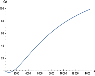
The purpose of this section is to numerically determine the function $f_{y}(Z)$ for negative $Z$, checking each step against the analytic results of the previous section. Because $Z(z)$ vanishes for $z=z_{*}\simeq 0.0880$ one cannot exactly reproduce the $\Lambda$CDM model in the range $0\leq z<z_{*}$ so we must also quantify the extent that the modified Friedman equation (15) causes the expansion history to deviate from the $\Lambda$CDM expansion history. Our technique for finding $f_{y}(Z)$ is to first determine it and $Z(z)$ numerically as functions of $z$ for $z\geq z_{*}$. We then invert the relation between $z$ and $Z$ to construct $z(Z)$, and use this to find $f_{y}$ as a function of $Z$, both numerically and by fitting to an analytic function. The section closes with a numerical evolution of the modified Friedman equation (15) in the range $0<z<z_{*}$ to determine how much the Hubble parameter deviates from that of the $\Lambda$CDM model.

4.1 Converting to $z$ and factoring out $\alpha$ and $\Omega_{\rm c}$

Figure 1: Graphs of $s(z)$ for $z_{*}<z<z_{\rm tr}$ (left) and for $z_{\rm tr}<z<4000$ (right).

We can entirely absorb the factors of $\alpha$ and $\Omega_{\rm c}$ in equations (25) and (26) by changing the independent variable to $z$ and rescaling the dependent variables as,

$$f(z)\equiv-\frac{f_{y}(Z)}{\alpha^{2}\Omega_{c}}\quad,\quad s(z)\equiv\frac{\sqrt{-Z}}{\alpha}\quad,\quad g(z)\equiv\int_{z}^{\infty}\frac{f^{\prime}(z^{\prime})dz^{\prime}}{(1\!+\!z^{\prime})s^{\prime}(z^{\prime})\widetilde{H}(z^{\prime})}\;.$$ (53)

With these definitions equations (25) and (26) become,

$$s(z)=(1\!+\!z)^{3}\!\!\int_{z}^{\infty}\!\!dz^{\prime}\,\frac{[\Omega_{\rm r}(1\!+\!z^{\prime})^{4}+\frac{1}{2}\Omega_{\rm m}(1\!+\!z^{\prime})^{3}-\Omega_{\Lambda}]}{(1\!+\!z^{\prime})^{4}\,\widetilde{H}(z^{\prime})}\;,$$ (54)

$$\frac{1}{2}f(z)+\frac{\widetilde{H}(z)f^{\prime}(z)}{2s^{\prime}(z)}+\widetilde{H}^{2}(z)g(z)=\frac{1}{12}(1\!+\!z)^{3}\;.$$ (55)

Equation (55) requires an initial condition which we take from the large $z$ limiting form of $f(z)\rightarrow\frac{1}{33}(1+z)^{3}$.

Figure 2: Graphs of $s(z)$ for $z_{*}<z<z_{\rm tr}$ (left) and for $z_{\rm tr}<z<100$ (right). The dotted line on the left shows the analytic formula (57), minus an offset of $\Delta s=\frac{1}{2}$ introduced to make the two curves distinguishable. The dotted line on the right displays the analytic formula (56), minus an offset of $\Delta s=10$ introduced to make the two curves distinguishable.

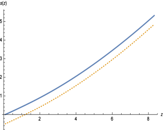
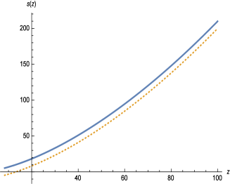
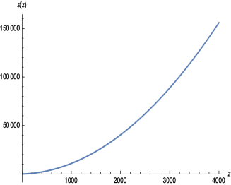
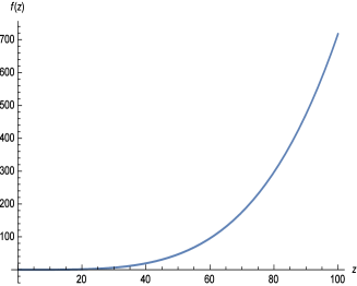
Figure 1 shows $s(z)$ over a large range of redshifts. Our previous work provided good analytic approximations for $s(z)$ — expressions (28) and (41) — depending upon whether $z$ is larger or smaller than the redshift of radiation-vacuum equality $z_{\rm tr}\equiv(\frac{\Omega_{\Lambda}}{\Omega{\rm m}})^{\frac{1}{4}}-1\simeq 8.32$,

$$z>z_{\rm tr} \!\!\!\!\Longrightarrow\!\!\!\! s(z)=\frac{\sqrt{\Omega_{\rm r}}(1\!+\!z)^{3}}{1\!+\!z_{\rm eq}}\Biggl{\{}\frac{1}{3}\Bigl{[}1+\frac{1\!+\!z_{\rm eq}}{1\!+\!z}\Bigr{]}^{\frac{3}{2}}+\Bigl{[}1+\frac{1\!+\!z_{\rm eq}}{1\!+\!z}\Bigr{]}^{\frac{1}{2}}-\frac{4}{3}\Biggr{\}},\qquad$$ (56)

$$z<z_{\rm tr} \!\!\!\!\Longrightarrow\!\!\!\! s(z)=\frac{\sqrt{\Omega_{\Lambda}}}{3y^{2}}\Biggl{\{}(2Y\!+\!5Y^{3})\sqrt{1\!+\!Y^{2}}-4Y^{4}-2\ln\Bigl{[}Y\!+\!\sqrt{1\!+\!Y^{2}}\,\Bigr{]}$$ (57)

$$\hskip 142.26378pt-y\sqrt{1\!+\!y^{2}}+2\ln\Bigl{[}y\!+\!\sqrt{1\!+\!y^{2}}\,\Bigr{]}\Biggr{\}}.\qquad$$

Here the redshift of matter-vacuum equality is $z_{\Lambda}\equiv(\frac{\Omega_{\Lambda}}{\Omega_{\rm m}})^{\frac{1}{3}}$ and we define $Y\equiv\sqrt{\frac{1+z_{\rm tr}}{1+z_{\rm eq}}}\simeq 0.0526$ and $y(z)\equiv(\frac{1+z_{\Lambda}}{1+z})^{\frac{3}{2}}$. Figure 2 shows that expressions (56-57) are in excellent agreement with the exact result (54). In fact, we had to offset the analytic formulae in order to distinguish them from the exact result! The same is not at all true for the asymptotic series expansions (29) and (42),

$${\rm Large}\,z \!\!\!\!\Longrightarrow\!\!\!\! s(z)=\sqrt{\Omega_{\rm r}}\,(1\!+\!z)^{2}\Biggl{\{}1+\frac{1}{24}x^{2}-\frac{1}{32}x^{3}+O\Bigl{(}x^{4}\Bigr{)}\Biggr{\}},$$ (58)

$${\rm Small}\,z \!\!\!\!\Longrightarrow\!\!\!\! s(z)=\frac{\sqrt{\Omega_{\Lambda}}}{3y_{*}^{2}}\Biggl{\{}-1.496\!\times\!\Delta y-1.036\!\times\!\Delta y^{2}+O\Bigl{(}\Delta y^{3}\Bigr{)}\Biggr{\}},$$ (59)

where $x(z)\equiv\frac{1+z_{\rm eq}}{1+z}$, $y_{*}\equiv y(z_{*})\simeq 1.318$ and $\Delta y\equiv y-y_{*}<0$. Figure 3 shows that the large $z$ series (58) is only valid for $z\mathrel{\raise 1.29167pt\hbox{$>$\kern-7.5pt\lower 4.30554pt\hbox{$\sim$}}}2000$, and the small $z$ series (59) is only valid for $z\mathrel{\raise 1.29167pt\hbox{$<$\kern-7.5pt\lower 4.30554pt\hbox{$\sim$}}}\frac{1}{2}$.

Figure 3: Graphs of $s(z)$ for $z_{*}<z<z_{\rm tr}$ (left) and for $1000<z<4000$ (right). The dashed line on the left shows the small $z$ series expansion (59) while the dashed line on the right shows the large $z$ series expansion (58).

Figure 4: Graphs of $f(z)$ for $z_{*}<z<1000$ (left) and for $1000<z<10000$ (right). The dashed line on the right-hand graph also shows the asymptotic series (60).

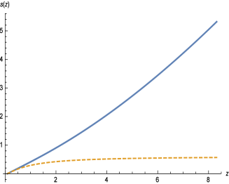
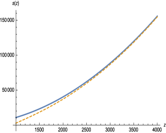
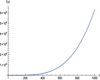
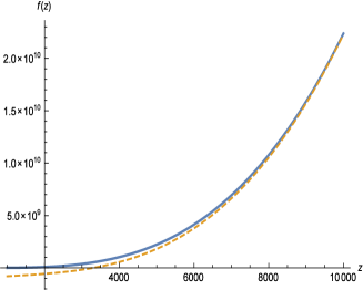
Evolving $f(z)$ with equation (55) is more challenging than numerically integrating $s(z)$ with (54). First, there is no analogue of the good analytic approximations (56-57) we were able to get for $s(z)$. Our previous work — expressions (34) and (49) — does imply asymptotic series expansions for large and small $z$,

$${\rm Large}\,z \!\!\!\!\Longrightarrow\!\!\!\! f(z)=\frac{(1\!+\!z)^{3}}{33}\Biggl{\{}1-x+\frac{83}{88}x^{2}-\frac{231}{256}x^{3}+O\Bigl{(}x^{4}\Bigr{)}\Biggr{\}},$$ (60)

$${\rm Small}\,z \!\!\!\!\Longrightarrow\!\!\!\! f(z)=\frac{(1\!+\!z_{\Lambda})^{3}}{36y_{*}^{2}}\Biggl{\{}1.143\!\times\!\Delta y-0.7373\!\times\!\Delta y^{2}+O\Bigl{(}\Delta y^{3}\Bigr{)}\Biggr{\}}.\qquad$$ (61)

However, one can see from Figures 4 and 5 that these series approximations are only accurate for $z\mathrel{\raise 1.29167pt\hbox{$>$\kern-7.5pt\lower 4.30554pt\hbox{$\sim$}}}5000$ and for $z\mathrel{\raise 1.29167pt\hbox{$<$\kern-7.5pt\lower 4.30554pt\hbox{$\sim$}}}1$, respectively.

Figure 5: Graphs of $f(z)$ for $z_{*}<z<20$ (left) and for $z_{*}<z<100$ (right). The dashed line on the left also shows the asymptotic series (61).

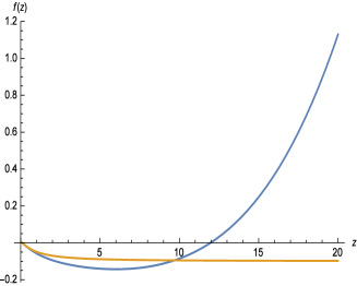
A worse problem is that numerical solution of (55) is unstable. We can evolve from large $z$ to small, starting from the excellent series approximation (60), but the result tends to diverge for small $z$. The better strategy turns out to be evolving from small $z$ to large, starting from $f(z_{*})=0$. To facilitate this procedure one must extract $g_{*}\equiv g(z_{*})$ from $g(z)$,

$$g(z)=g_{*}-\int_{z_{*}}^{z}\!\!\frac{f^{\prime}(z^{\prime})dz^{\prime}}{(1\!+\!z^{\prime})s^{\prime}(z^{\prime})\widetilde{H}(z^{\prime})}\;.$$ (62)

When this is done, evolving to arbitrarily large $z$ produces a solution which seems to reach the form (60), but then grows in magnitude like $z^{2+2\sqrt{3}}$, either in the positive or negative direction. The correct value of $g_{*}\simeq 0.1807$ is found by seeking the point at which the asymptotic form changes sign.

4.2 Solving for $f_{y}(Z)$ Numerically

Figure 6: Graphs of $f(z)$ versus $s$ for $0<s<20$ (left) and for $0<s<100$ (right). The dashed line on the left gives the asymptotic series expansion (63).

Figure 7: Graphs of $f(z)$ versus $s$ for $0<s<10^{3}$ (left) and for $10^{5}<s<10^{6}$ (right). The dashed line on the right gives the asymptotic series expansion (64).

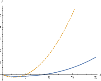
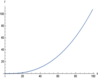
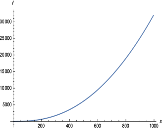
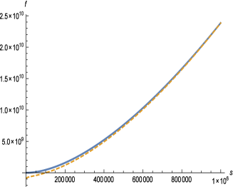
This is really just a matter of using our previous results for $s(z)$ and $f(z)$ to plot $f(z)$ as a function of $s$. Figures 6 and 7 show the results for small and large values of $s$, respectively. For the smallest ($0<s<20$) and largest ($10^{3}<s<10^{6}$) ranges we also show the comparison with the analytic asymptotic series expansion which follow from the work of section 3,

$${\rm Small}\;s \Longrightarrow f(z)=\frac{(1\!+\!z_{\Lambda})^{3}}{12}\Biggl{\{}\frac{A\,s}{\sqrt{\Omega_{\Lambda}}}+\frac{B\,s^{2}}{\Omega_{\Lambda}}+O\Bigl{(}\frac{s^{3}}{\Omega_{\Lambda}^{\frac{3}{2}}}\Bigr{)}\Biggr{\}}\qquad,$$ (63)

$${\rm Large}\;s \!\!\!\Longrightarrow\!\!\! f(z)=\frac{1}{33}\Bigl{(}\frac{s}{\sqrt{\Omega_{\rm r}}}\Bigr{)}^{\frac{3}{2}}\!\Biggl{\{}\!1\!-\!\frac{1}{\sqrt{\sigma}}\!+\!\frac{155}{176}\frac{1}{\sigma}\!-\!\frac{625}{768}\frac{1}{\sigma^{\frac{3}{2}}}\!+\!O\Bigl{(}\frac{1}{\sigma^{2}}\Bigr{)}\!\Biggr{\}},\qquad$$ (64)

where $A\simeq-0.764$ and $B\simeq+0.127$ and we define $\sigma(s)$ as,

$$\sigma(s)\equiv\frac{s}{\sqrt{\Omega_{\rm r}}(1\!+\!z_{\rm eq})^{2}}\;.$$ (65)

Points to note are that the small $s$ series (63) breaks down for $s\mathrel{\raise 1.29167pt\hbox{$>$\kern-7.5pt\lower 4.30554pt\hbox{$\sim$}}}\frac{1}{4}$, and the large $s$ series (64) breaks down for $s\mathrel{\raise 1.29167pt\hbox{$<$\kern-7.5pt\lower 4.30554pt\hbox{$\sim$}}}300,000$.

4.3 Fitting $f_{y}(Z)$ to an Analytic Form

Figure 8: Graphs of the ratios of $f(z)$ to the asymptotic series expansions (63-64) versus $s$ for the ranges $0<s<\frac{1}{4}$ (on the left) and for $10^{5}<s<10^{6}$ (on the right).

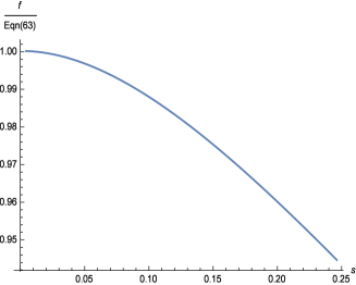
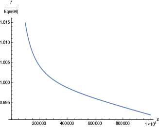
A better measure of the accuracy of the asymptotic series expansions (63-64) is gained by plotting the ratio of the numerical result for $f(z)$ divided by the expansions. Figure 8 shows this. The failure of the very large $s$ ratio to exactly approach unity is due to instability of our numerical determination of $f(z)$, as explained before. However, the deviations for $\frac{1}{4}<s<300,000$ represent the transition between the two asymptotic forms which we would like to fit to an analytic function.

Figure 9: The left hand graph shows $f(z)$ versus $s(z)$ in the region $0<s<20$. The dashed line shows the best fit quadratic in this same region. The right hand graph is a log-log plot of $f(z)$ versus $s$ in the range $10^{2}<s<10^{6}$.

Figure 10: Variation of the coefficients $\gamma(s)$ and $\delta(s)$ in equation (68). The left hand graph shows how the fitted coefficient $\gamma$ varies slowly with the midpoint of a small region used to make the fit. The right hand graph shows the same thing for the coefficient $\delta$.

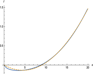
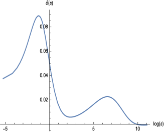
We are dealing with a smooth function whose qualitative features are shown in Figure 9:

• The small $s$ regime is well fit by $\gamma s+\delta s^{2}$, but the coefficients $\gamma$ and $\delta$ evolve slowly as shown in Figure 10; and

• The large $s$ regime is well fit by a power law which changes slowly from $s^{2}$ for moderate values of $s$ to $s^{\frac{3}{2}}$ for large values of $s$.

We can find a reasonable ansatz by making a plausible interpolation of the asymptotic series in curly brackets of expression (64), with $\sigma(s)$ from (65),

$$1-\frac{1}{\sqrt{\sigma}}+\frac{155}{176}\frac{1}{\sigma}-\frac{625}{768}\frac{1}{\sigma^{\frac{3}{2}}}+O\Bigl{(}\frac{1}{\sigma^{2}}\Bigr{)}\longrightarrow\frac{1}{1+\frac{1}{\sqrt{\sigma}}+\frac{21}{176\,\sigma}+\frac{443}{8448\,\sigma^{\frac{3}{2}}}}\;.\qquad$$ (66)

The right hand side of (66) has the same large $\sigma$ series expansion as the left hand side, but it behaves like $\frac{8448}{443}\sigma^{\frac{3}{2}}$ for small $\sigma$. Hence we might define,

$$f_{\rm lg}(s)\equiv\frac{1}{33}\Bigl{(}\frac{s}{\Omega_{\rm r}}\Bigr{)}^{\frac{3}{2}}\!\times\!\frac{1}{1+\frac{1}{\sqrt{\sigma(s)}}+\frac{21}{176\,\sigma(s)}+\frac{443}{8448\,\sigma^{\frac{3}{2}}(s)}}\;.$$ (67)

This function will recover the asymptotic large $s$ behavior, and go to zero rapidly for small $s$. Then a reasonable ansatz for the full function is,

$$f(z)=\gamma(s)\!\times\!s+\delta(s)\!\times\!s^{2}+f_{\rm lg}(s)\;,$$ (68)

The general shapes of $\gamma(s)$ and $\delta(s)$ in Figure 10 motivate our fits. For $\gamma(s)$ a single rational function suffices; $\delta(s)$ is better described by the sum of two terms, each of which falls off exponentially. Our results are,

$$\gamma(s) = \frac{(\frac{5}{29}\!+\!\frac{s}{144})(\frac{s}{1440}\!-\!1)}{1+\frac{s}{10000}+(\frac{s}{5700})^{2}+(\frac{s}{25000})^{3}}\;,$$ (69)

$$\delta(s) = \frac{\frac{1}{29}\!+\!\frac{1}{9}\sqrt{s}\!-\!\frac{1}{6}s\!+\!\frac{2}{9}s^{\frac{3}{2}}+s^{2}}{1+25s^{\frac{11}{4}}\exp[\frac{1}{12}s]}+\frac{\frac{s}{4000}\!-\!100(\frac{s}{4000})^{2}\!+\!10^{4}(\frac{s}{4000})^{3}}{1+33\!\times\!10^{4}(\frac{s}{4000})^{\frac{32}{11}}\exp[\frac{s}{4000}]}\;.$$ (70)

More complicated polynomials would of course be more accurate.

4.4 Quantifying the Disagreement for $0<z<z_{*}$

Figure 11: The left hand graph shows the evolution of $\Phi(z)\equiv\frac{\dot{\phi}}{6H_{0}}$ in the actual model. The right hand graph shows $h(z)\equiv\frac{H}{H_{0}}$ in the actual model.

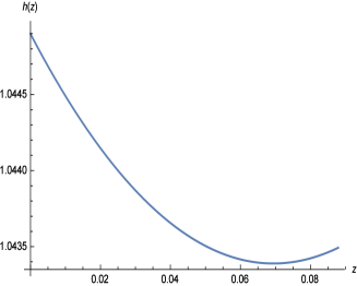
We have shown how to choose the function $f_{y}(Z)$ so as to exactly reproduce the $\Lambda$CDM expansion history for all redshifts greater than $z_{*}\simeq 0.0880$. One cannot do the same for the small range $0<z<z_{*}$ because $s(z)$ changes sign from positive to negative in this region, whereas $Z=-\alpha^{2}s^{2}$ is negative for all $z$. Hence $f_{y}(Z)$ takes values already used to fit redshifts for $z>z_{*}$. This means the very late time expansion history deviates from the $\Lambda$CDM model.

We can use the MOND cosmological equations (12), (14) and (15) to derive a system of local, first order differential equations for $\dot{\phi}$ and $H$ which can be evolved inward from $z=z_{*}$, starting with the initial conditions $\dot{\phi}_{*}=0$ and $H_{*}=H_{0}\widetilde{H}(z_{*})$. Our labor is reduced by some preliminary rescalings,

$$\dot{\phi}\equiv 6H_{0}\!\times\!\Phi(z)\qquad,\qquad H\equiv H_{0}\!\times\!h(z)\;.$$ (71)

Then equation (12) implies,

$$\Phi^{\prime}=\frac{3\Phi}{1\!+\!z}+h^{\prime}-\frac{h}{1\!+\!z}\;.$$ (72)

Dividing equation (15) by $3H_{0}^{2}$ gives,

$$h^{2}(z)+\frac{6f_{y}(Z)}{\alpha^{2}}+12h(z)\Phi(z)f^{\prime}_{y}(Z)+24h^{2}(z)\!\!\int_{z}^{\infty}\!\!dz^{\prime}\,\frac{\Phi(z^{\prime})f^{\prime}_{y}(Z^{\prime})}{(1\!+\!z^{\prime})h(z^{\prime})}$$ (73)

$$\hskip 170.71652pt=\Omega_{\rm r}(1\!+\!z)^{4}+\Omega_{\rm b}(1\!+\!z)^{3}+\Omega_{\Lambda}\;.\qquad$$

Dividing by $h^{2}(z)$ and differentiating with respect to $z$ will eliminate the integration. Before giving the result it is worthwhile making some simplifications based on the fact that the redshifts we seek to understand are very near $z=0$. First, the radiation term to the right of (73) can be dropped. Second, there is no point to using more than the first two terms of the small $s$ expansion (63) for $f_{y}(Z)$,

$$-\frac{f_{y}(Z)}{\alpha^{2}\Omega_{\rm c}} \!\!\!\!\simeq\!\!\!\! \frac{(1\!+\!z_{\Lambda})^{3}}{12}\Biggl{\{}\frac{A\sqrt{-Z}}{\alpha\sqrt{\Omega_{\Lambda}}}-\frac{BZ}{\alpha^{2}\Omega_{\Lambda}}\Biggr{\}}=\frac{(1\!+\!z_{\Lambda})^{3}}{12}\Biggl{\{}\tilde{a}\Phi+\tilde{b}\Phi^{2}\Biggr{\}},\qquad$$ (74)

$$-\frac{f^{\prime}_{y}(Z)}{\alpha^{2}\Omega_{\rm c}} \!\!\!\!\simeq\!\!\!\! \frac{(1\!+\!z_{\Lambda})^{3}}{12}\Biggl{\{}-\frac{A}{2\alpha\sqrt{-\Omega_{\Lambda}Z}}-\frac{B}{\alpha^{2}\Omega_{\Lambda}}\Biggr{\}}=\frac{(1\!+\!z_{\Lambda})^{3}}{12\alpha^{2}}\Biggl{\{}-\frac{\tilde{a}}{2\Phi}-\tilde{b}\Biggr{\}},\qquad$$ (75)

where we define $\tilde{a}\equiv\frac{A}{\sqrt{\Omega_{\Lambda}}}\simeq-0.9192$ and $\tilde{b}\equiv\frac{B}{\Omega_{\Lambda}}\simeq+0.1843$. It is also convenient to define $\tilde{c}\equiv\Omega_{\rm c}(1+z_{\Lambda})^{3}\simeq+0.5824$. With these simplifications the final evolution equation for $h(z)$ is,

$$\Biggl{\{}-\frac{\tilde{a}}{2h}-\frac{\tilde{b}\Phi}{h}+\frac{\tilde{a}\Phi}{h^{2}}+\frac{2[\Omega_{\rm b}(1\!+\!z)^{3}\!+\!\Omega_{\Lambda}]}{\tilde{c}h^{2}}\Biggr{\}}h^{\prime}+\Biggl{\{}-\frac{\tilde{a}}{2h}+\tilde{b}\Biggr{\}}\Phi^{\prime}$$ (76)

$$\hskip 199.16928pt=\frac{\tilde{a}\!+\!2\tilde{b}\Phi}{1\!+\!z}+\frac{3\Omega_{\rm b}(1\!+\!z)^{2}}{\tilde{c}h}\;.\qquad$$

Figure 11 shows the results of evolving equations (72) and (76) inward from $z=z_{*}$, starting with the initial conditions $\Phi(z_{*})=0$ and $h(z_{*})=\widetilde{H}(z_{*})\simeq 1.043$. The evolution of $\Phi(z)$ is not significantly different from the $\Lambda$CDM model, however, the evolution of $h(z)$ differs markedly. Instead of continuing to decline to the $\Lambda$CDM value of $\widetilde{H}(0)=1$, $h(z)$ turns around and increases slightly to $h(0)\simeq 1.045$. The increase is not large but halting the decrease may provide an explanation for the increasingly significant tension between inferences of $H_{0}$ based on data from large $z$ [25] (cosmic ray background anisotropies and baryon acoustic oscillations) and from small $z$ [26] (Hubble plots),

$${\rm Large}\;z \Longrightarrow H_{0}=\Bigl{(}67.74\pm 0.46\Bigr{)}~{}\frac{\rm km}{\rm s~{}Mpc}\;,$$ (77)

$${\rm Small}\;z \Longrightarrow H_{0}=\Bigl{(}73.24\pm 1.74\Bigr{)}~{}\frac{\rm km}{\rm s~{}Mpc}\;.$$ (78)

The model was defined using the large $z$ numbers [25], which moves our prediction for the current Hubble parameter closer to the small $z$ result (78),

$$1.045\times\Bigl{(}67.74\pm 0.46\Bigr{)}~{}\frac{\rm km}{\rm s~{}Mpc}=\Bigl{(}70.79\pm 0.48\Bigr{)}\frac{\rm km}{\rm s~{}Mpc}\;.$$ (79)

5 Discussion

This paper concerns a metric-based realization of MOND [18, 19] whose Lagrangian (3) involves an algebraic function $f_{y}(Z)$ of a nonlocal scalar (4). For gravitationally bound systems $Z[g]$ is typically positive and the form of $f_{y}(Z)$ is well constrained by the Tully-Fisher relation, weak lensing and solar system tests. For cosmological systems the metric’s temporal variation is typically more important than its spatial dependence, which causes $Z[g]$ to be negative. Our goal in this paper has been to determine how the function $f_{y}(Z)$ must depend upon negative $Z$ so as to reproduce the $\Lambda$CDM expansion history without dark matter.

We did not quite succeed because specializing to the $\Lambda$CDM geometry does not result in a one-to-one function $Z(z)$ for all $z>0$. For large $z$ the function $Z(z)$ is negative and its magnitude decreases as $z$ decreases. However, $Z(z)$ touches zero at $z_{*}\simeq 0.0880$ and then returns to negative values in the range $0<z<z_{*}$. Therefore, we can only choose $f_{y}(Z)$ to enforce the $\Lambda$CDM expansion history for $z>z_{*}$. In this region we determined $f_{y}(Z)$ numerically, and then showed that a simple combination of analytic functions (67-70) provides an excellent fit, with $Z\equiv-\alpha^{2}s^{2}$ and $f_{y}(Z)\equiv-\alpha^{2}\Omega_{\rm c}f(z)$. We also demonstrated that the model’s deviation from $\Lambda$CDM in the range $0<z<z_{*}$ causes the current Hubble parameter to be about 4.5% larger than for the $\Lambda$CDM model. This would reduce (from $3.2\sigma$ to only $1.4\sigma$) the tension which currently exists between inferences of $H_{0}$ which are based on data from large $z$ [25] and those based on small $z$ data [26].

Cosmology offers an interesting venue for comparing nonlocal MOND with the $\Lambda$CDM model. Both models incorporate the known densities of radiation and baryonic matter, and both models assume an absurdly small cosmological constant. In both cases the remaining component of the Friedmann equation is abstracted to cosmology from an explanation for very large and weakly gravitationally bound structures. In both cases there is no definitive derivation of this remaining component from fundamental theory although possibilities exist. One major difference is that the $\Lambda$CDM model requires only the single free parameter $\Omega_{\rm c}$ to describe the remaining component of the Friedmann equation whereas nonlocal cosmology has a free function $f_{y}(Z)$ for $Z<0$. On the other hand, the function required does not seem outlandish.

The most reasonable conclusion is probably that the cosmology of nonlocal MOND will stand or fall depending on what it predicts now that the function $f_{y}(Z)$ has been fixed. The model can be used to study things such as the response to recent disturbances of gravitationally bound systems and to perturbations around the background cosmology. The analogy is how numerically determining the distortion function [27] of a nonlocal model of dark energy [28] has facilitated detailed studies of structure formation in that model [29, 30, 31]. We do not yet know how these studies will turn out for the nonlocal realization of MOND, however, a crucially important point is that the function $f_{y}(Z)$ is NOT small for cosmology. This means that the MOND corrections have a reasonable chance to reproduce what dark matter does in general relativity.

The surprising (and wonderful) fact that MOND corrections are large for cosmology was not expected by many who attempted to guess the form a relativistic extension of MOND might take. These people made the reasonable assumption that MOND corrections to cosmology should be negligible because they are small for gravitationally bound systems, and because even those small corrections entirely disappear when the curvature reaches values far smaller than it has taken in cosmological history. This assumption fails for two reasons:

• The invariant (4) becomes large in cosmology; and

• The function $f_{y}(Z)$ is not suppressed for large negative $Z$ the way it is for large positive $Z$.

The first point is a consequence of invariance. The phenomenology of MOND dictates (4) as the simplest form for $Z[g]$ [18, 19], and just evaluating this functional for the $\Lambda$CDM cosmology happens to produce numerically large results. Of course the second point resulted from how we choose to extend the function $f_{y}(Z)$ for negative $Z$. However, it is important to realize that this decision makes sense if one conceives of MOND as derived from the vacuum polarization of inflationary gravitons [20]. Those gravitons have cosmological scales so it is entirely reasonable to expect strong effects on cosmological scales but only weak effects on smaller scales.

Acknowledgements

We are grateful for conversations and correspondence with C. Deffayet, S. Deser and G. Esposito-Farese. This work was partially supported by NSF grant PHY-1506513 and by the Institute for Fundamental Theory at the University of Florida.

References

- [1] C. M. Will, Living Rev. Rel. 9, 3 (2006) doi:10.12942/lrr-2006-3 [gr-qc/0510072].
- [2] B. P. Abbott et al. [LIGO Scientific and Virgo Collaborations], Phys. Rev. Lett. 116, no. 6, 061102 (2016) doi:10.1103/PhysRevLett.116.061102 [arXiv:1602.03837 [gr-qc]].
- [3] S. S. McGaugh, Astrophys. J. 632, 859 (2005) doi:10.1086/432968 [astro-ph/0506750].
- [4] M. Kaplinghat and M. S. Turner, Astrophys. J. 569, L19 (2002) doi:10.1086/340578 [astro-ph/0107284].
- [5] K. C. Freeman, Astrophys. J. 160, 811 (1970). doi:10.1086/150474
- [6] R. Sancisi, [IAU Symp. 220, 233 (2004)] [astro-ph/0311348].
- [7] R. H. Sanders, arXiv:0806.2585 [astro-ph].
- [8] L. J. Rosenberg, Proc. Nat. Acad. Sci. (2015). doi:10.1073/pnas.1308788112
- [9] D. S. Akerib et al. [LUX Collaboration], Phys. Rev. Lett. 116, no. 16, 161302 (2016) doi:10.1103/PhysRevLett.116.161302 [arXiv:1602.03489 [hep-ex]].
- [10] D. S. Akerib et al., arXiv:1608.07648 [astro-ph.CO].
- [11] M. Milgrom, Astrophys. J. 270, 365 (1983). doi:10.1086/161130
- [12] M. Milgrom, Astrophys. J. 270, 371 (1983). doi:10.1086/161131
- [13] M. Milgrom, Astrophys. J. 270, 384 (1983). doi:10.1086/161132
- [14] R. H. Sanders and S. S. McGaugh, Ann. Rev. Astron. Astrophys. 40, 263 (2002) doi:10.1146/annurev.astro.40.060401.093923 [astro-ph/0204521].
- [15] B. Famaey and S. McGaugh, Living Rev. Rel. 15, 10 (2012) doi:10.12942/lrr-2012-10 [arXiv:1112.3960 [astro-ph.CO]].
- [16] J. D. Bekenstein, Phys. Rev. D 70, 083509 (2004) Erratum: [Phys. Rev. D 71, 069901 (2005)] doi:10.1103/PhysRevD.70.083509, 10.1103/PhysRevD.71.069901 [astro-ph/0403694].
- [17] J. W. Moffat, JCAP 0603, 004 (2006) doi:10.1088/1475-7516/2006/03/004 [gr-qc/0506021].
- [18] C. Deffayet, G. Esposito-Farese and R. P. Woodard, Phys. Rev. D 84, 124054 (2011) doi:10.1103/PhysRevD.84.124054 [arXiv:1106.4984 [gr-qc]].
- [19] C. Deffayet, G. Esposito-Farese and R. P. Woodard, Phys. Rev. D 90, no. 6, 064038 (2014) Addendum: [Phys. Rev. D 90, no. 8, 089901 (2014)] doi:10.1103/PhysRevD.90.089901, 10.1103/PhysRevD.90.064038 [arXiv:1405.0393 [astro-ph.CO]].
- [20] R. P. Woodard, Can. J. Phys. 93, no. 2, 242 (2015) doi:10.1139/cjp-2014-0156 [arXiv:1403.6763 [astro-ph.CO]].
- [21] N. C. Tsamis and R. P. Woodard, Class. Quant. Grav. 31, 185014 (2014) doi:10.1088/0264-9381/31/18/185014 [arXiv:1405.6281 [gr-qc]].
- [22] S. Nojiri and S. D. Odintsov, Phys. Lett. B 659, 821 (2008) doi:10.1016/j.physletb.2007.12.001 [arXiv:0708.0924 [hep-th]].
- [23] S. Deser and R. P. Woodard, JCAP 1311, 036 (2013) doi:10.1088/1475-7516/2013/11/036 [arXiv:1307.6639 [astro-ph.CO]].
- [24] R. P. Woodard, Found. Phys. 44, 213 (2014) doi:10.1007/s10701-014-9780-6 [arXiv:1401.0254 [astro-ph.CO]].
- [25] P. A. R. Ade et al. [Planck Collaboration], arXiv:1502.01589 [astro-ph.CO].
- [26] A. G. Riess et al., Astrophys. J. 826, no. 1, 56 (2016) doi:10.3847/0004-637X/826/1/56 [arXiv:1604.01424 [astro-ph.CO]].
- [27] C. Deffayet and R. P. Woodard, JCAP 0908, 023 (2009) doi:10.1088/1475-7516/2009/08/023 [arXiv:0904.0961 [gr-qc]].
- [28] S. Deser and R. P. Woodard, Phys. Rev. Lett. 99, 111301 (2007) doi:10.1103/PhysRevLett.99.111301 [arXiv:0706.2151 [astro-ph]].
- [29] S. Park and S. Dodelson, Phys. Rev. D 87, no. 2, 024003 (2013) doi:10.1103/PhysRevD.87.024003 [arXiv:1209.0836 [astro-ph.CO]].
- [30] S. Dodelson and S. Park, Phys. Rev. D 90, 043535 (2014) doi:10.1103/PhysRevD.90.043535 [arXiv:1310.4329 [astro-ph.CO]].
- [31] S. Park and A. Shafieloo, arXiv:1608.02541 [astro-ph.CO].