Optimizing Content Caching to Maximize the Density of Successful Receptions in Device-to-Device Networking

Derya Malak, Mazin Al-Shalash, and Jeffrey G. Andrews Parts of the manuscript were presented at the 2014 IEEE Globecom Workshops [1] and at the 2015 IEEE ICC Workshops [2].D. Malak and J. G. Andrews are with the Wireless and Networking Communications Group (WNCG), The University of Texas at Austin, Austin, TX 78701 USA (email: deryamalak@utexas.edu; jandrews@ece.utexas.edu). M. Al-Shalash is with Huawei Technologies, Plano, TX 75075 USA (e-mail: mshalash@huawei.com).This research has been supported by Huawei. Manuscript last revised: .
Abstract

Device-to-device (π–£πŸ€π–£π–£πŸ€π–£\sf{D2D}) communication is a promising approach to optimize the utilization of air interface resources in 5G networks, since it allows decentralized opportunistic short-range communication. For π–£πŸ€π–£π–£πŸ€π–£\sf{D2D} to be useful, mobile nodes must possess content that other mobiles want. Thus, intelligent caching techniques are essential for π–£πŸ€π–£π–£πŸ€π–£\sf{D2D}. In this paper we use results from stochastic geometry to derive the probability of successful content delivery in the presence of interference and noise. We employ a general transmission strategy where multiple files are cached at the users and different files can be transmitted simultaneously throughout the network. We then formulate an optimization problem, and find the caching distribution that maximizes the density of successful receptions (DSRDSR\rm{DSR}) under a simple transmission strategy where a single file is transmitted at a time throughout the network. We model file requests by a Zipf distribution with exponent Ξ³rsubscriptπ›Ύπ‘Ÿ\gamma_{r}, which results in an optimal caching distribution that is also a Zipf distribution with exponent Ξ³csubscript𝛾𝑐\gamma_{c}, which is related to Ξ³rsubscriptπ›Ύπ‘Ÿ\gamma_{r} through a simple expression involving the path loss exponent. We solve the optimal content placement problem for more general demand profiles under Rayleigh, Ricean and Nakagami small-scale fading distributions. Our results suggest that it is required to flatten the request distribution to optimize the caching performance. We also develop strategies to optimize content caching for the more general case with multiple files, and bound the DSRDSR\rm{DSR} for that scenario.

I Introduction

Wireless networks are experiencing a well-known ever-rising demand for enhanced high rate data services, in particular wireless video, which is forecast to consume around 70% of wireless bandwidth by 2019 [3]. Non-real-time video in particular is expected to comprise half of this amount [4], and comprises large files that can be cached in the network. Meanwhile, preliminary π–£πŸ€π–£π–£πŸ€π–£\sf{D2D} techniques have been standardized by 3GPP to allow decentralized file sharing and public safety applications [5]. π–£πŸ€π–£π–£πŸ€π–£\sf{D2D} is intriguing since it allows increased spatial reuse and possibly very high rate communication without increased network infrastructure or new spectrum, but is only viable when the mobile users have content that other nearby users want. Thus, it is clear that smart content caching is essential for π–£πŸ€π–£π–£πŸ€π–£\sf{D2D}.

Caching popular content is a well known technique to reduce resource usage, and increase content access speed and availability [6]. Infrastructure-based caching can reduce delay and when done at the network edge, also reduce the impact on the backhaul network, which in many cases is the bottleneck in wireless networks [7]. However, this type of caching does not reduce the demand on spectral resources. To gain spectral reuse and increase the area spectral efficiency, the content must be cached on wireless devices themselves, which allows short-range communication which is independent of the network infrastructure. π–£πŸ€π–£π–£πŸ€π–£\sf{D2D} communication can enable proximity-based applications involving discovering and communicating with nearby devices [8]. Synchronized distributed network architectures for π–£πŸ€π–£π–£πŸ€π–£\sf{D2D} communications are designed, e.g., FlashLinQ [9] and ITLinQ [10], and caching is shown to provide increased spectral reuse in π–£πŸ€π–£π–£πŸ€π–£\sf{D2D}-enabled networks [11]. Although order optimal solutions for optimal content placement is known under certain channel conditions [12, 13, 14], it is not known how to best cache content in a π–£πŸ€π–£π–£πŸ€π–£\sf{D2D} network. Intuitively, popular content should be seeded into the users’ limited storage resources in a way that maximizes the probability that a given π–£πŸ€π–£π–£πŸ€π–£\sf{D2D} device can find a desired file within its radio range. Exploring this problem quantitively is the goal of this paper.

I-A Related Work

Different aspects of π–£πŸ€π–£π–£πŸ€π–£\sf{D2D} content distribution are studied. Scalability in ad hoc networks is considered [15], where decentralized algorithms for message forwarding are proposed by considering a Zipf product form model for message preferences. Throughput scaling laws with caching have been widely studied [16, 17, 18]. Optimal collaboration distance, Zipf distribution for content reuse, best achievable scaling for the expected number of active π–£πŸ€π–£π–£πŸ€π–£\sf{D2D} interference-free collaboration pairs for different Zipf exponents is studied [19]. With a heuristic choice (Zipf) of caching distribution for Zipf distributed requests, the optimal collaboration distance [20] and the Zipf exponent to maximize number of π–£πŸ€π–£π–£πŸ€π–£\sf{D2D} links are determined [17]. However, in general, the caching pmf is not necessarily same as the request pmf. This brings us to the one of the main objectives in this paper, which is to find the best caching pmf that achieves the best density of successful receptions (DSRDSR\rm{DSR}) in π–£πŸ€π–£π–£πŸ€π–£\sf{D2D} networks.

Under the classical protocol model of ad hoc networks [21], for a grid network model, with fixed cache size M𝑀M, as the number of users n𝑛n and the number of files mπ‘šm become large with n​M≫mmuch-greater-thanπ‘›π‘€π‘šnM\gg m, the order optimal111The order optimality in [12, 22] is in the sense of a throughput-outage tradeoff due to simple model used. caching distribution is studied and the per-node throughput is shown to behave as Ξ˜β€‹(M/m)Ξ˜π‘€π‘š\Theta(M/m) [12, 22]. The network diameter is shown to scale as n𝑛\sqrt{n} for a multi-hop scenario [13]. It is shown that local multi-hop yields per-node throughput scaling as Ξ˜β€‹(M/m)Ξ˜π‘€π‘š\Theta(\sqrt{M/m}) [14].

Spatial caching for a client requesting a large file that is stored at the caches with limited storage, is studied [23]. Using Poisson point process (𝖯𝖯𝖯𝖯𝖯𝖯\sf{PPP}) to model the user locations, optimal geographic content placement and outage in wireless networks are studied [24]. The probability that the typical user finds the content in one of its nearby base stations (𝖑𝖲𝖑𝖲\sf{BS})s is optimized using the distribution of the number of 𝖑𝖲𝖑𝖲\sf{BS}s simultaneously covering a user [25]. Performance of randomized caching in π–£πŸ€π–£π–£πŸ€π–£\sf{D2D} networks from a DSRDSR\rm{DSR} maximization perspective has not been studied, which we study in this paper.

Although the work conducted in [17, 19] focused on the optimal caching distribution to maximize the average number of connections, the system model was overly simplistic. They assumed a cellular network where each 𝖑𝖲𝖑𝖲\sf{BS} serves the users in a square cell. The cell is divided into small clusters. π–£πŸ€π–£π–£πŸ€π–£\sf{D2D} communications are allowed within each cluster. To avoid intra-cluster interference, only one transmitter-receiver pair per cluster is allowed, and it does not introduce interference for other clusters. In this paper, we aim to overcome these serious limitations using a more realistic π–£πŸ€π–£π–£πŸ€π–£\sf{D2D} network model that captures the simultaneous transmissions where there is no restriction in the number of π–£πŸ€π–£π–£πŸ€π–£\sf{D2D} pairs.

I-B Contributions

This paper develops optimal content caching strategies that aim to maximize the average density of successful receptions so as to address the demands of π–£πŸ€π–£π–£πŸ€π–£\sf{D2D} receivers. The contributions are as follows.

Physical channel modeling using 𝖯𝖯𝖯𝖯𝖯𝖯\sf{PPP}. We introduce the network model in Sect. II, in which the locations of the π–£πŸ€π–£π–£πŸ€π–£\sf{D2D} users are modeled as a homogeneous 𝖯𝖯𝖯𝖯𝖯𝖯\sf{PPP}. Different from the grid-based model in [12, 22], we consider the actual physical channel model. 𝖯𝖯𝖯𝖯𝖯𝖯\sf{PPP} modeling makes our analysis tractable because unlike the cluster-based model in [20], where only a pair of users are allowed to communicate in a square region, we require no constraint on the link distance and allow a random number of simultaneous transmissions. All analysis is for a typical mobile node which is permissible in a homogeneous 𝖯𝖯𝖯𝖯𝖯𝖯\sf{PPP} by Slivnyak’s theorem [26]. The interference due to simultaneously active transmitters, noise and the small-scale Rayleigh fading are incorporated into the analysis. Any transmission is successful as long as the Signal-to-Interference-plus-Noise Ratio (𝖲𝖨𝖭𝖱𝖲𝖨𝖭𝖱\sf{SINR}) is above a threshold.

Density of successful receptions (DSRDSR\rm{DSR}). We propose a new file caching strategy exploiting stochastic geometry and the results of [27], and we introduce the concept of the density of successful receptions (DSRDSR\rm{DSR}). Although in this paper, we do not investigate the throughput-outage tradeoff as in [12, 22], the DSRDSR\rm{DSR} is closely related to the outage probability, obtained through the scaling of the coverage, i.e., the complement of the outage probability, with the number of receivers per unit area.

Optimal caching distribution to maximize the DSRDSR\rm{DSR} for the sequential multi-file model. We study a randomized transmission model for π–£πŸ€π–£π–£πŸ€π–£\sf{D2D} users with storage size 111 in Sect. II. We propose techniques for randomized content caching based on the possible ways of prioritizing different files. In Sect. III, we start with a baseline model with single file to determine the optimal fractions of transmitters Ξ³1subscript𝛾1\gamma_{1} and receivers Ξ³2subscript𝛾2\gamma_{2} in the π–£πŸ€π–£π–£πŸ€π–£\sf{D2D} network model with 𝖯𝖯𝖯𝖯𝖯𝖯\sf{PPP} distributed user locations that maximizes the DSRDSR\rm{DSR}. In Sect. IV, we consider the more general sequential multi-file transmission scenario, where we investigate the maximum DSRDSR\rm{DSR} in terms of the optimal fractions of Ξ³1subscript𝛾1\gamma_{1} and Ξ³2subscript𝛾2\gamma_{2} derived in Sect. III, to determine the DSRDSR\rm{DSR}, and optimize the caching pmf based on the randomized model.

Small-scale fading DSRDSR\rm{DSR} results. We formulate an optimization problem in Sect. IV-A to find the best caching distribution that maximizes the DSRDSR\rm{DSR} under a simple transmission strategy where single file is transmitted at a time throughout the network, assuming user demands are modeled by a Zipf distribution with exponent Ξ³rsubscriptπ›Ύπ‘Ÿ\gamma_{r}. This scheme yields a certain fraction of users to be active at a time based on the distribution of the requests. In Sect. IV-B, we optimize the DSRDSR\rm{DSR} of users for the multi-file setup, where the small-scale fading is Rayleigh distributed. We consider several special cases corresponding to 1) small but non-zero noise, 2) arbitrary noise and 3) an approximation for arbitrary noise allowing the path loss exponent Ξ±=4𝛼4\alpha=4. For case 1), we show that the optimal caching strategy also has a Zipf distribution but with exponent Ξ³c=Ξ³rΞ±/2+1subscript𝛾𝑐subscriptπ›Ύπ‘Ÿπ›Ό21\gamma_{c}=\frac{\gamma_{r}}{\alpha/2+1} where Ξ±>2𝛼2\alpha>2. For case 2), we show that the same result holds based on an approximation of the 𝖲𝖨𝖭𝖱𝖲𝖨𝖭𝖱\sf{SINR} coverage justified numerically in Sect. IV-B. This relation implies that Ξ³csubscript𝛾𝑐\gamma_{c} is smaller than Ξ³rsubscriptπ›Ύπ‘Ÿ\gamma_{r}, i.e., the caching distribution should be more uniform compared to the request distribution, yet more popular files should be cached at a higher number of π–£πŸ€π–£π–£πŸ€π–£\sf{D2D} users. For case 3), we obtain a distribution similar to Benford’s law (detailed in Sect. IV-B) that optimizes the caching pmf. We also extend our results to the β€œgeneral request distributions”, and show that cases 1) and 2) are also valid for Ricean and Nakagami fading distributions in Sect. IV-B.

In general, the optimal DSRDSR\rm{DSR} and the optimal caching distribution might not be tractable. Therefore, assuming the request and caching probabilities are known a priori, we weight the caching pmf to provide iterative techniques to optimize the DSRDSR\rm{DSR} under different settings. We propose caching strategies that consider maximizing the DSRDSR\rm{DSR} of the least desired file and of all files as detailed in Sect. V-B.

Optimal caching distribution to maximize the DSRDSR\rm{DSR} for the simultaneous multi-file model. In Sect. VI, we extend our study to the simultaneous transmissions of different files and define popularity-based and global strategies. The popularity-based strategy is in favor of the transmission of popular files and discards unpopular files. On the other hand, the global strategy schedules all the files simultaneously, which leads to lower coverage than the sequential model does. Optimization of the DSRDSR\rm{DSR} in these cases is very intricate compared to the case of sequential modeling. Therefore, we numerically compare the proposed caching models in Sect. VI, and observe that the optimal solutions become skewed towards the most popular content in the network. Thus, we infer that under different models, the optimal caching distribution may not be a Zipf distribution as also found in [12, 13, 14].

Insights. Our results show that the optimal caching strategy exhibits less locality of the reference (abbreviated as locality) compared to the input stream of requests, i.e., the demand distribution222The performance of demand-driven caching depends on the locality exhibited by the stream of requests. The more skewed the popularity pmf, (i) the stronger the locality and the smaller the miss rate of the cache[28], and (ii) good cache replacement strategies are expected to produce an output stream of requests exhibiting less locality than the input stream of requests [29]. In [28], authors showed that (i) and (ii) hold for caches operating under random on-demand replacement algorithms.. We also analyze the special case of Ξ±=4𝛼4\alpha=4 using a tight approximation for standard Gaussian QQ\rm Q-function. Using this approach we show that the optimal caching distribution can be approximated by Benford’s law, which is a special bounded case of Zipf’s law [30]. In Sect. VII, we validate that both Zipf distribution and Benford’s law have very similar distributional characteristics, further validating the generality of the results. For the multiple file case, we extend our results by finding lower and upper bounds for the DSRDSR\rm{DSR} in Sect. V. Simulations show that the bounds are very accurate approximations for particular Ξ³rsubscriptπ›Ύπ‘Ÿ\gamma_{r} values.

II System Model

We consider a mobile network model in which π–£πŸ€π–£π–£πŸ€π–£\sf{D2D} users are spatially distributed as a homogeneous 𝖯𝖯𝖯𝖯𝖯𝖯\sf{PPP} ΦΦ\Phi of density Ξ»πœ†\lambda, where a randomly selected user can transmit or receive information.
Refer to caption
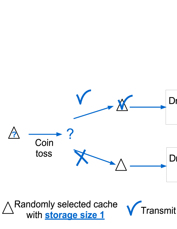
Figure 1: Randomized caching model.

In the multiple file scenario, the randomized caching model we propose is shown in Fig. 1. The model can be summarized as follows. At any time slot, only a fraction of the π–£πŸ€π–£π–£πŸ€π–£\sf{D2D} users scheduled. Any user transmits with probability Ξ³1subscript𝛾1\gamma_{1} and receives with probability Ξ³2=1βˆ’Ξ³1subscript𝛾21subscript𝛾1\gamma_{2}=1-\gamma_{1} independently of other users. Each user has a cache with storage size 111. If it is selected as a receiver at a time slot, it draws a sample from the request distribution pr​(β‹…)subscriptπ‘π‘Ÿβ‹…p_{r}(\cdot), which is assumed to be Zipf distributed. If it is selected as transmitter at a time slot, it draws a sample from the caching distribution pc​(β‹…)subscript𝑝𝑐⋅p_{c}(\cdot). The selection of request distribution and the optimization of caching distribution will be detailed in Sect. IV. At any time slot, each receiver is scheduled based on closest transmitter association.

A system model for the π–£πŸ€π–£π–£πŸ€π–£\sf{D2D} content distribution network with multiple files is illustrated in Fig. 2. For multiple file case, different from the single file case, where the π–£πŸ€π–£π–£πŸ€π–£\sf{D2D} content distribution network is like a downlink cellular network since nearest transmitter has the content, a farther transmitter is often the one with the file required by the receiver.

Refer to caption
Figure 2: System model for π–£πŸ€π–£π–£πŸ€π–£\sf{D2D} users with multiple files. Each receiver is associated to its closest transmitter that contains the requested file, where TX​(k)TXk\rm TX(k) and RX​(k)RXk\rm RX(k) denote the set of transmitters and receivers corresponding to file kπ‘˜k. For illustration purposes, different types are separated on the plot. However, transmissions of different files can occur simultaneously.

General models for the multi-cell 𝖲𝖨𝖭𝖱𝖲𝖨𝖭𝖱\sf{SINR} using stochastic geometry were developed in [27], where the downlink coverage probability was derived as:

pcov​(T,Ξ»,Ξ±)β‰œβ„™β€‹[𝖲𝖨𝖭𝖱>T]=Ο€β€‹Ξ»β€‹βˆ«0∞eβˆ’Ο€β€‹Ξ»β€‹r​β​(T,Ξ±)βˆ’ΞΌβ€‹T​σ2​rΞ±/2​dr,β‰œsubscript𝑝covTπœ†π›Όβ„™delimited-[]𝖲𝖨𝖭𝖱Tπœ‹πœ†superscriptsubscript0superscripteπœ‹πœ†r𝛽Tπ›Όπœ‡Tsuperscript𝜎2superscriptr𝛼2dr\displaystyle p_{\rm cov}({\rm T},\lambda,\alpha)\triangleq\mathbb{P}[\sf{SINR}>\rm T]=\pi\lambda\int_{0}^{\infty}{e^{-\pi\lambda r\beta({\rm T},\alpha)-\mu\rm T\sigma^{2}r^{\alpha/2}}\,\mathrm{d}r}, (1)

where β​(T,Ξ±)=2​(μ​T)2αα​𝔼​[g2α​(Γ​(βˆ’2/Ξ±,μ​T​g)βˆ’Ξ“β€‹(βˆ’2/Ξ±))]𝛽T𝛼2superscriptπœ‡T2𝛼𝛼𝔼delimited-[]superscript𝑔2𝛼Γ2π›Όπœ‡T𝑔Γ2𝛼\beta({\rm T},\alpha)=\frac{2(\mu{\rm T})^{\frac{2}{\alpha}}}{\alpha}\mathbb{E}\big{[}g^{\frac{2}{\alpha}}(\Gamma(-2/\alpha,\mu{\rm T}g)-\Gamma(-2/\alpha))\big{]}. The expectation is with respect to the interference power distribution g𝑔g, the transmit power is 1/ΞΌ1πœ‡1/\mu, and Signal-to-Noise Ratio (𝖲𝖭𝖱𝖲𝖭𝖱\sf{SNR}) is defined at a distance of r=1π‘Ÿ1r=1 and is 𝖲𝖭𝖱=1/(μ​σ2)𝖲𝖭𝖱1πœ‡superscript𝜎2{\sf{SNR}}=1/(\mu\sigma^{2}). A summary of the symbol definitions and important network parameters are given in Table I.

Definition 1.

Density of successful receptions (DSRDSR\rm{DSR}). The performance of a randomly chosen receiver is determined by its 𝖲𝖨𝖭𝖱𝖲𝖨𝖭𝖱\sf{SINR} coverage. For the homogeneous 𝖯𝖯𝖯𝖯𝖯𝖯\sf{PPP} ΦΦ\Phi with density Ξ»πœ†\lambda, let Ξ³1subscript𝛾1\gamma_{1} fraction of all users be the transmitter process Ξ¦tsubscriptΦ𝑑\Phi_{t}, and Ξ³2subscript𝛾2\gamma_{2} fraction of users be the receiver process Ξ¦rsubscriptΞ¦π‘Ÿ\Phi_{r}, where 0<Ξ³1,Ξ³2<1formulae-sequence0subscript𝛾1subscript𝛾210<\gamma_{1},\gamma_{2}<1. The coverage probability of a randomly chosen receiver is pcov​(T,λ​γ1,Ξ±)subscript𝑝covTπœ†subscript𝛾1𝛼p_{\rm cov}({\rm T},\lambda\gamma_{1},\alpha), which is the same for all receivers, and the total average number of receivers is proportional to the density λ​γ2πœ†subscript𝛾2\lambda\gamma_{2}. Hence, the DSRDSR\rm{DSR}, which denotes the mean number of successful receptions per unit area, equals

𝖣𝖲𝖱=λ​γ2​pcov​(T,λ​γ1,Ξ±)=λ​γ2​(π​λ​γ1β€‹βˆ«0∞eβˆ’Ο€β€‹Ξ»β€‹Ξ³1​r​β​(T,Ξ±)βˆ’ΞΌβ€‹T​σ2​rΞ±/2​dr),π–£π–²π–±πœ†subscript𝛾2subscript𝑝covTπœ†subscript𝛾1π›Όπœ†subscript𝛾2πœ‹πœ†subscript𝛾1superscriptsubscript0superscriptπ‘’πœ‹πœ†subscript𝛾1π‘Ÿπ›½Tπ›Όπœ‡Tsuperscript𝜎2superscriptr𝛼2differential-dπ‘Ÿ\displaystyle{\sf{DSR}}=\lambda\gamma_{2}p_{\rm cov}({\rm T},\lambda\gamma_{1},\alpha)=\lambda\gamma_{2}\Big{(}\pi\lambda\gamma_{1}\int\nolimits_{0}^{\infty}{e^{-\pi\lambda\gamma_{1}r\beta({\rm T},\alpha)-\mu\rm T\sigma^{2}r^{\alpha/2}}\,\mathrm{d}r}\Big{)}, (2)

where pcov​(T,λ​γ1,Ξ±)subscript𝑝covTπœ†subscript𝛾1𝛼p_{\rm cov}({\rm T},\lambda\gamma_{1},\alpha) is obtained by combining (1) with the thinning property of the 𝖯𝖯𝖯𝖯𝖯𝖯\sf{PPP}, i.e., Ξ¦tsubscriptΦ𝑑\Phi_{t}, which is obtained through the thinning of ΦΦ\Phi, is a homogeneous 𝖯𝖯𝖯𝖯𝖯𝖯\sf{PPP} with density λ​γ1πœ†subscript𝛾1\lambda\gamma_{1} [31, Ch. 1].

We consider the generalized file caching problem in 𝖯𝖯𝖯𝖯𝖯𝖯\sf{PPP} networks where every user randomly requests or caches some files based on the availabilities. Our goal is to maximize the DSRDSR\rm{DSR} in (2) for single file and multiple files. We discuss the details of our optimization problem in Sects. III and IV.

III DSRDSR\rm{DSR} For a Single File

We first assume that there is a single file in the network. The single file case is the baseline model for the more general multi-file model presented in Sect. IV. Sampled uniformly at random from the 𝖯𝖯𝖯𝖯𝖯𝖯\sf{PPP} ΦΦ\Phi, a fraction Ξ³1subscript𝛾1\gamma_{1} of the users form the process Ξ¦tsubscriptΦ𝑑\Phi_{t} of the users possessing the file, and a fraction Ξ³2subscript𝛾2\gamma_{2} of the users form the process Ξ¦rsubscriptΞ¦π‘Ÿ\Phi_{r} of the users who want the same file. The receivers communicate with the nearest transmitter while all other transmitters act as interferers, and each transmitter can serve multiple receivers. A receiver is in coverage when its 𝖲𝖨𝖭𝖱𝖲𝖨𝖭𝖱\sf{SINR} from its nearest transmitter is larger than some threshold TT\rm T. Given the total density of receivers is given by λ​γ2πœ†subscript𝛾2\lambda\gamma_{2}, and each receiver is successfully covered with probability pcov​(T,λ​γ1,Ξ±)subscript𝑝covTπœ†subscript𝛾1𝛼p_{\rm cov}({\rm T},\lambda\gamma_{1},\alpha), the DSRDSR\rm{DSR}, i.e., 𝖣𝖲𝖱𝖣𝖲𝖱\sf{DSR}, is given by their product. In the single file scenario, since there is only 1 file being transmitted in the network, there is no caching pmf. Our objective in this section is to determine the optimal fractions of transmitters Ξ³1subscript𝛾1\gamma_{1} and receivers Ξ³2subscript𝛾2\gamma_{2} in the 𝖯𝖯𝖯𝖯𝖯𝖯\sf{PPP} network that maximizes the DSRDSR\rm{DSR}. In Sect. IV, we consider the multiple file transmission scenario, where we use the optimal fractions of transmitters and receivers Ξ³1subscript𝛾1\gamma_{1} and Ξ³2subscript𝛾2\gamma_{2}, respectively, derived in this section, to determine the DSRDSR\rm{DSR}, and optimize the caching pmf based on the randomized model outlined in Sect. II. We formulate the following optimization problem to determine Ξ³1subscript𝛾1\gamma_{1} and Ξ³2subscript𝛾2\gamma_{2}:

π–£π–²π–±βˆ—=superscript𝖣𝖲𝖱absent\displaystyle{\sf{DSR}^{*}}= maxΞ³1>0,Ξ³2>0formulae-sequencesubscript𝛾10subscript𝛾20\displaystyle\underset{\gamma_{1}>0,\,\gamma_{2}>0}{\max} λ​γ2​pcov​(T,λ​γ1,Ξ±)πœ†subscript𝛾2subscript𝑝covTπœ†subscript𝛾1𝛼\displaystyle\lambda\gamma_{2}p_{\rm cov}({\rm T},\lambda\gamma_{1},\alpha) (3)
      s.t. Ξ³1+Ξ³2=a,0<a≀1,formulae-sequencesubscript𝛾1subscript𝛾2π‘Ž0π‘Ž1\displaystyle\gamma_{1}+\gamma_{2}=a,\quad 0<a\leq 1,

where pcov​(T,λ​γ1,Ξ±)subscript𝑝covTπœ†subscript𝛾1𝛼p_{\rm cov}({\rm T},\lambda\gamma_{1},\alpha) is the coverage probability of a typical user, and a≀1π‘Ž1a\leq 1 is the total fraction of transmitting and receiving users in a 𝖯𝖯𝖯𝖯𝖯𝖯\sf{PPP} network ΦΦ\Phi with density Ξ»πœ†\lambda.

Symbol Definition
TT\rm T; Ξ±>2𝛼2\alpha>2 𝖲𝖨𝖭𝖱𝖲𝖨𝖭𝖱\sf{SINR} threshold; Path loss exponent
Ξ³1subscript𝛾1\gamma_{1}; Ξ³2subscript𝛾2\gamma_{2} Fraction of transmitting users; fraction of receiving users
ΦΦ\Phi; Ξ¦tsubscriptΦ𝑑\Phi_{t}; Ξ¦rsubscriptΞ¦π‘Ÿ\Phi_{r} Homogeneous 𝖯𝖯𝖯𝖯𝖯𝖯\sf{PPP} of all π–£πŸ€π–£π–£πŸ€π–£\sf{D2D} users; transmitter process; receiver process
Ξ»πœ†\lambda; Ξ»tsubscriptπœ†π‘‘\lambda_{t} Intensity of ΦΦ\Phi; intensity of Ξ¦tsubscriptΦ𝑑\Phi_{t}
ΞΌβˆ’1superscriptπœ‡1\mu^{-1}; Οƒ2superscript𝜎2\sigma^{2} The constant transmit power; Noise variance
g∼exp⁑(ΞΌ)similar-toπ‘”πœ‡g\sim\exp(\mu) Interference power distribution
Ξ³rsubscriptπ›Ύπ‘Ÿ\gamma_{r}; Ξ³csubscript𝛾𝑐\gamma_{c} Zipf request parameter; Zipf caching parameter
M𝑀M; 111 Size of the file catalog; storage size of any user
pr​(β‹…)subscriptπ‘π‘Ÿβ‹…p_{r}(\cdot); pc​(β‹…)subscript𝑝𝑐⋅p_{c}(\cdot) Popularity pmf; caching pmf
pcov​(T,Ξ»,Ξ±)subscript𝑝covTπœ†π›Όp_{\rm cov}({\rm T},\lambda,\alpha) Coverage probability for the sequential transmission model
𝒫cov​(T,Ξ»,Ξ±)subscript𝒫covTπœ†π›Ό\mathcal{P}_{\rm cov}({\rm T},\lambda,\alpha) Coverage probability for the general transmission model
β​(T,Ξ±)𝛽T𝛼\beta({\rm T},\alpha) A function of interference in the exponent of pcovsubscript𝑝covp_{\rm cov}
FB​(β‹…)subscript𝐹𝐡⋅F_{B}(\cdot) The pmf of the Benford’s distribution
𝖣𝖲𝖱𝖣𝖲𝖱\sf{DSR} Density of successful receptions
𝖣𝖲𝖱𝖲;𝖣𝖲𝖱𝖯;𝖣𝖲𝖱𝖦subscript𝖣𝖲𝖱𝖲subscript𝖣𝖲𝖱𝖯subscript𝖣𝖲𝖱𝖦\sf{DSR_{S}};\sf{DSR_{P}};\sf{DSR_{G}} Sequential; popularity-based; global model 𝖣𝖲𝖱𝖣𝖲𝖱\sf{DSR}
QQ\rm Q-function The tail probability of the standard normal distribution
Ξ˜β€‹(β‹…)Ξ˜β‹…\Theta(\cdot); o​(β‹…)π‘œβ‹…o(\cdot) Big O notation; Little-o notation
TABLE I: Important network parameters.
Lemma 1.

The fraction of transmitters should be less than that of receivers, i.e., the solution of (3) satisfies the following relation: Ξ³1<a/2<Ξ³2<a≀1subscript𝛾1π‘Ž2subscript𝛾2π‘Ž1\gamma_{1}<a/2<\gamma_{2}<a\leq 1.

Proof.

See Appendix -A. ∎

Lemma 2.

The maximum DSRDSR\rm{DSR} for arbitrary noise and Ξ±=4𝛼4\alpha=4 is given by

π–£π–²π–±βˆ—=λ​(aβˆ’Ξ³1)/(1Ξ³1​[1Ξ³1βˆ’1aβˆ’Ξ³1]​2​μ​T​σ2(π​λ)2​β​(T,4)+β​(T,4)).superscriptπ–£π–²π–±πœ†π‘Žsubscript𝛾11subscript𝛾1delimited-[]1subscript𝛾11π‘Žsubscript𝛾12πœ‡π‘‡superscript𝜎2superscriptπœ‹πœ†2𝛽T4𝛽T4\displaystyle{\sf{DSR}^{*}}={\lambda(a-\gamma_{1})}\Big{/}{\Big{(}\frac{1}{\gamma_{1}}\left[\frac{1}{\gamma_{1}}-\frac{1}{a-\gamma_{1}}\right]\frac{{2\mu T\sigma^{2}}}{(\pi\lambda)^{2}\beta({\rm T},4)}+\beta({\rm T},4)\Big{)}}.
Proof.

See Appendix -B. ∎

Corollary 1.

Low 𝖲𝖭𝖱𝖲𝖭𝖱\sf{SNR} case, Ξ±=4𝛼4\alpha=4. As Οƒ2β†’βˆžβ†’superscript𝜎2\sigma^{2}\to\infty, the coverage can be approximated as pcov​(T,Ξ»,Ξ±)=ℙ​[𝖲𝖨𝖭𝖱>T]β‰ˆβ„™β€‹[𝖲𝖭𝖱>T]=Ο€β€‹Ξ»β€‹βˆ«0∞eβˆ’Ο€β€‹Ξ»β€‹rβˆ’ΞΌβ€‹T​σ2​rΞ±/2​drsubscript𝑝covTπœ†π›Όβ„™delimited-[]𝖲𝖨𝖭𝖱Tβ„™delimited-[]𝖲𝖭𝖱Tπœ‹πœ†superscriptsubscript0superscripteπœ‹πœ†rπœ‡Tsuperscript𝜎2superscriptr𝛼2drp_{\rm cov}({\rm T},\lambda,\alpha)=\mathbb{P}[\sf{SINR}>\rm T]\approx\mathbb{P}[\sf{SNR}>\rm T]=\pi\lambda\int_{0}^{\infty}{e^{-\pi\lambda r-\mu\rm T\sigma^{2}r^{\alpha/2}}\,\mathrm{d}r}. Hence, the maximum DSRDSR\rm{DSR} is given as

π–£π–²π–±βˆ—=λ​(aβˆ’Ξ³1)/(1Ξ³1​[1Ξ³1βˆ’1aβˆ’Ξ³1]​2​μ​T​σ2(π​λ)2+1),superscriptπ–£π–²π–±πœ†π‘Žsubscript𝛾11subscript𝛾1delimited-[]1subscript𝛾11π‘Žsubscript𝛾12πœ‡π‘‡superscript𝜎2superscriptπœ‹πœ†21\displaystyle{\sf{DSR}^{*}}={\lambda(a-\gamma_{1})}\Big{/}{\Big{(}\frac{1}{\gamma_{1}}\left[\frac{1}{\gamma_{1}}-\frac{1}{a-\gamma_{1}}\right]\frac{{2\mu T\sigma^{2}}}{(\pi\lambda)^{2}}+1\Big{)}}, (4)

where optimal Ξ³1subscript𝛾1\gamma_{1} satisfies aβˆ’3​a​γ1+3​γ12Ξ³13​(aβˆ’Ξ³1)=(π​λ)24​μ​T​σ2π‘Ž3π‘Žsubscript𝛾13superscriptsubscript𝛾12superscriptsubscript𝛾13π‘Žsubscript𝛾1superscriptπœ‹πœ†24πœ‡π‘‡superscript𝜎2\frac{a-3a\gamma_{1}+3\gamma_{1}^{2}}{\gamma_{1}^{3}(a-\gamma_{1})}=\frac{(\pi\lambda)^{2}}{{4\mu T\sigma^{2}}}.

Corollary 2.

No noise (degenerative) case. For no noise, pcov​(T,Ξ»,Ξ±)=β​(T,Ξ±)βˆ’1subscript𝑝covTπœ†π›Όπ›½superscriptT𝛼1p_{\rm cov}({\rm T},\lambda,\alpha)=\beta({\rm T},\alpha)^{-1}. Maximum DSRDSR\rm{DSR} for single file for 0<a≀10π‘Ž10<a\leq 1, Rayleigh fading, no noise, and Ξ±>2𝛼2\alpha>2 is π–£π–²π–±βˆ—=maxΞ³1>0​λ​(aβˆ’Ξ³1)​1β​(T,Ξ±)=λ​(aβˆ’Ξ³1βˆ—)β​(T,Ξ±)superscript𝖣𝖲𝖱subscript𝛾10πœ†π‘Žsubscript𝛾11𝛽Tπ›Όπœ†π‘Žsuperscriptsubscript𝛾1𝛽T𝛼{\sf{DSR}^{*}}=\underset{\gamma_{1}>0}{\max}\,\,\lambda(a-\gamma_{1})\frac{1}{\beta({\rm T},\alpha)}=\frac{\lambda(a-\gamma_{1}^{*})}{\beta({\rm T},\alpha)}, obtained for the optimal value of Ξ³1subscript𝛾1\gamma_{1}, i.e., Ξ³1βˆ—=Ξ΅>0superscriptsubscript𝛾1πœ€0\gamma_{1}^{*}=\varepsilon>0 so that there is one transmitter333In the no noise case the single file result is trivial. In multiple file case, there will be interference due to the simultaneous transmissions of multiple files, which will be discussed in Sect. IV..

Next, we consider the low noise approximation of the success probability that is more easily computable than the constant noise power expression and more accurate than the no noise approximation for Οƒ2=0superscript𝜎20\sigma^{2}=0. Using the expansion exp⁑(βˆ’x)=1βˆ’x+o​(x)π‘₯1π‘₯π‘œπ‘₯\exp(-x)=1-x+o(x) for Οƒ2β‰ 0superscript𝜎20\sigma^{2}\neq 0 as xβ†’0β†’π‘₯0x\to 0, the term pcov​(T,Ξ»,Ξ±)subscript𝑝covTπœ†π›Όp_{\rm cov}({\rm T},\lambda,\alpha) for small but non-zero noise case can be calculated after an integration by parts of (1) as follows

pcov​(T,Ξ»,Ξ±)=1β​(T,Ξ±)βˆ’ΞΌβ€‹T​σ2​(λ​π)βˆ’Ξ±2β​(T,Ξ±)Ξ±2+1​Γ​(1+Ξ±2)+o​(Οƒ2).subscript𝑝covTπœ†π›Ό1𝛽Tπ›Όπœ‡Tsuperscript𝜎2superscriptπœ†πœ‹π›Ό2𝛽superscriptT𝛼𝛼21Ξ“1𝛼2π‘œsuperscript𝜎2\displaystyle p_{\rm cov}({\rm T},\lambda,\alpha)=\frac{1}{\beta({\rm T},\alpha)}-\frac{\mu\rm T\sigma^{2}\left(\lambda\pi\right)^{-\frac{\alpha}{2}}}{\beta({\rm T},\alpha)^{\frac{\alpha}{2}+1}}\Gamma\left(1+\frac{\alpha}{2}\right)+o\left(\sigma^{2}\right).
Lemma 3.

The maximum DSRDSR\rm{DSR} for a single file for a=1π‘Ž1a=1, Rayleigh fading, small noise is equal to

π–£π–²π–±βˆ—=λ​αβ​(T,Ξ±)​[1Ξ±βˆ’(Ξ³1βˆ—βˆ’1)Ξ±+Ξ³1βˆ—β€‹(2βˆ’Ξ±)​o​(Οƒ2)].superscriptπ–£π–²π–±πœ†π›Όπ›½T𝛼delimited-[]1𝛼superscriptsubscript𝛾11𝛼superscriptsubscript𝛾12π›Όπ‘œsuperscript𝜎2\displaystyle{\sf{DSR}^{*}}=\frac{\lambda\alpha}{\beta({\rm T},\alpha)}\left[\frac{1}{\alpha}-\frac{(\gamma_{1}^{*}-1)}{\alpha+\gamma_{1}^{*}(2-\alpha)}o(\sigma^{2})\right].
Proof.

See Appendix -C. ∎

For Ξ±=4𝛼4\alpha=4, there is a closed form expression for β​(T,4)𝛽T4\beta({\rm T},4) as follows: β​(T,4)=1+T​arctan⁑(T)𝛽T41TT\beta({\rm T},4)=1+\sqrt{\rm T}\arctan(\sqrt{\rm T}), which we use for the derivation of Lemma 4.

Lemma 4.

The maximum DSRDSR\rm{DSR} for small but non-zero noise and Ξ±=4𝛼4\alpha=4 is

π–£π–²π–±βˆ—=2​λ​(aβˆ’Ξ³1)(1+T​arctan⁑(T))​[1βˆ’ΞΌβ€‹T​σ2​aμ​T​σ2​(2​aβˆ’Ξ³1)+o​(Οƒ2)]+o​(Οƒ2).superscript𝖣𝖲𝖱2πœ†π‘Žsubscript𝛾11TTdelimited-[]1πœ‡Tsuperscript𝜎2π‘Žπœ‡Tsuperscript𝜎22π‘Žsubscript𝛾1π‘œsuperscript𝜎2π‘œsuperscript𝜎2\displaystyle{\sf{DSR}^{*}}=\frac{2\lambda(a-\gamma_{1})}{(1+\sqrt{\rm T}\arctan(\sqrt{\rm T}))}\left[1-\frac{\mu{\rm T}\sigma^{2}a}{\mu{\rm T}\sigma^{2}(2a-\gamma_{1})+o(\sigma^{2})}\right]+o(\sigma^{2}). (5)
Proof.

See Appendix -D. ∎

Refer to caption

(a)

Refer to caption

(b)

Refer to caption

(c)

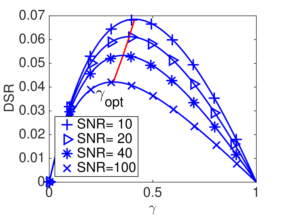
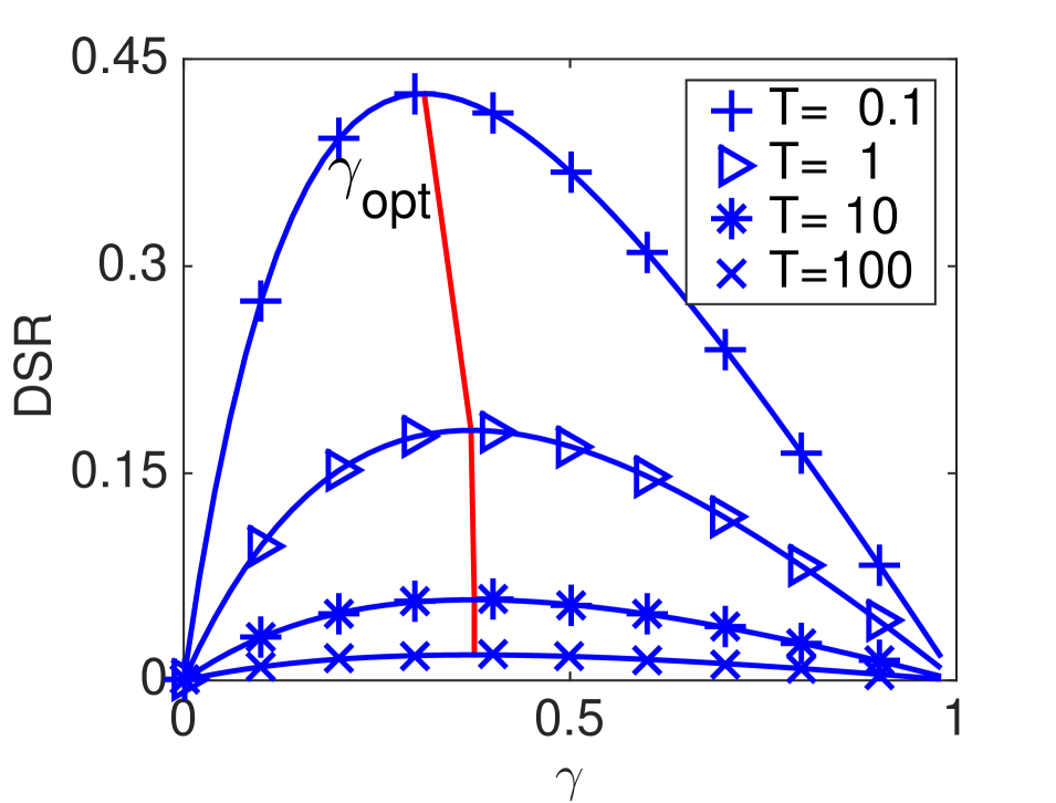
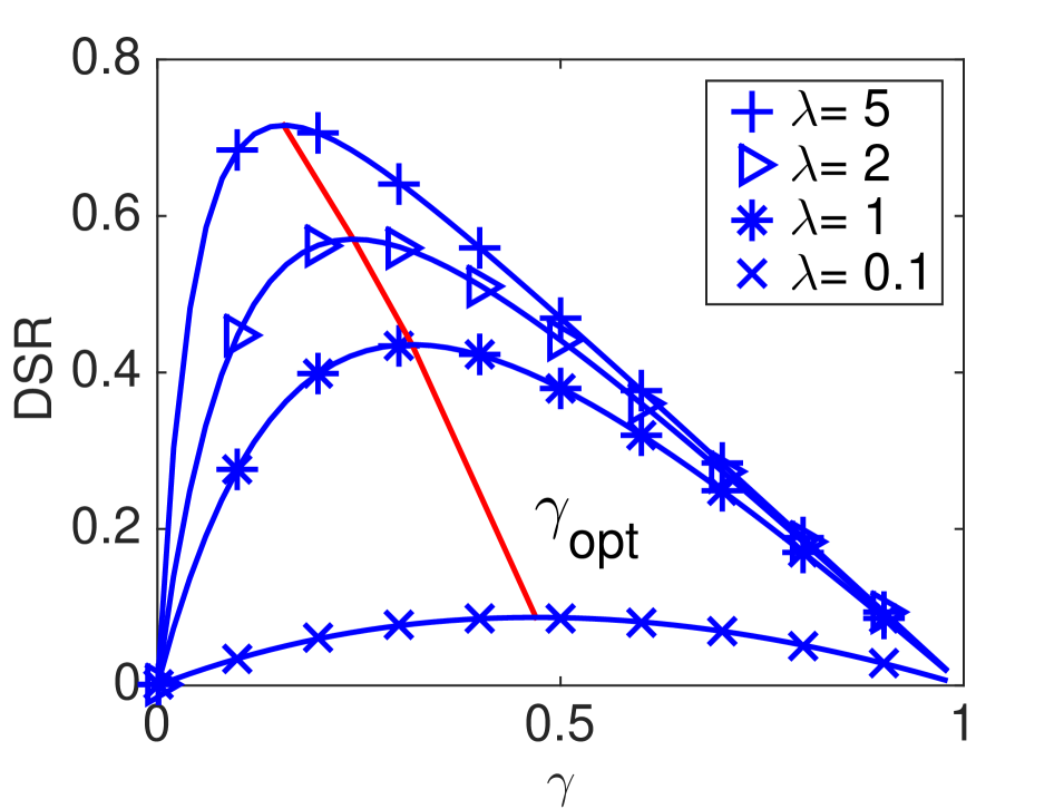
Figure 3: DSRDSR\rm{DSR} for single file versus γ𝛾\gamma with respect to 𝖲𝖭𝖱𝖲𝖭𝖱\sf{SNR}, TT\rm T and Ξ»πœ†\lambda. (a) DSRDSR\rm{DSR}, T=𝖲𝖭𝖱/𝟀T𝖲𝖭𝖱2\rm T=\sf{SNR}/2, Ξ»πœ†\lambda=0.1, where the dashed curves correspond to the respective Monte Carlo simulations, (b) DSRDSR\rm{DSR}, 𝖲𝖭𝖱=πŸ€πŸ’π–²π–­π–±20\sf{SNR}=20, Ξ»πœ†\lambda=0.1, and (c) DSRDSR\rm{DSR}, 𝖲𝖭𝖱=.1𝖲𝖭𝖱.1\sf{SNR}=.1, T=.05T.05\rm T=.05.

Discussion. In Fig. 3 (a), we illustrate the relation between π–£π–²π–±βˆ—superscript𝖣𝖲𝖱{\sf{DSR}^{*}} and 𝖲𝖭𝖱𝖲𝖭𝖱\sf{SNR} for T=𝖲𝖭𝖱/𝟀T𝖲𝖭𝖱2\rm T=\sf{SNR}/2, Ξ»πœ†\lambda=0.1. To simplify the notation, we assume that Ξ³1+Ξ³2=1subscript𝛾1subscript𝛾21\gamma_{1}+\gamma_{2}=1 and let Ξ³=Ξ³1𝛾subscript𝛾1\gamma=\gamma_{1} and Ξ³1βˆ—=Ξ³optsuperscriptsubscript𝛾1subscript𝛾opt\gamma_{1}^{*}=\gamma_{\mathrm{opt}}. As 𝖲𝖭𝖱𝖲𝖭𝖱\sf{SNR} increases for T=𝖲𝖭𝖱/𝟀T𝖲𝖭𝖱2\rm T=\sf{SNR}/2, the DSRDSR\rm{DSR} decreases and Ξ³optsubscript𝛾opt\gamma_{\mathrm{opt}} decreases. Note that the solid lines denote the simulation results for the 𝖯𝖯𝖯𝖯𝖯𝖯\sf{PPP} model. In Fig. 3 (b), the variation of π–£π–²π–±βˆ—superscript𝖣𝖲𝖱{\sf{DSR}^{*}} with respect to TT\rm T for 𝖲𝖭𝖱=πŸ£πŸ’π–²π–­π–±10\sf{SNR}=10, Ξ»πœ†\lambda=0.1 is shown. The coverage pcov​(T,λ​γ1,Ξ±)subscript𝑝covTπœ†subscript𝛾1𝛼p_{\rm cov}({\rm T},\lambda\gamma_{1},\alpha) is monotonically decreasing in TT\rm T and a concave increasing function of Ξ³1subscript𝛾1\gamma_{1}. For increasing TT\rm T, the value of DSRDSR\rm{DSR} becomes very small, and to maximize the DSRDSR\rm{DSR}, a higher fraction of the users should be transmitters (i.e., higher Ξ³1subscript𝛾1\gamma_{1}) to compensate the outage. For low T𝑇T, to maximize the DSRDSR\rm{DSR}, the fraction of the receivers Ξ³2subscript𝛾2\gamma_{2} should be higher. Therefore, as TT\rm T decreases, the DSRDSR\rm{DSR} increases and becomes right-skewed, but Ξ³optsubscript𝛾opt\gamma_{\mathrm{opt}} decreases only slightly, which is negligible444This follows from the separability assumption of pcov​(T,λ​γ1,Ξ±)subscript𝑝covTπœ†subscript𝛾1𝛼p_{\rm cov}({\rm T},\lambda\gamma_{1},\alpha) in λ​γ1πœ†subscript𝛾1\lambda\gamma_{1} and T𝑇T, thus insensitivity of the DSRDSR\rm{DSR} maximization problem to the value of T𝑇T, which is further detailed in Assumption 1 of Sect. IV-B, and verified in Appendix -F.. Thus, we conclude that Ξ³optsubscript𝛾opt\gamma_{\mathrm{opt}} is largely invariant to TT\rm T and mainly determined by 𝖲𝖭𝖱𝖲𝖭𝖱\sf{SNR}. In Fig. 3 (c), we show the variation of π–£π–²π–±βˆ—superscript𝖣𝖲𝖱{\sf{DSR}^{*}} with Ξ»πœ†\lambda. The DSRDSR\rm{DSR} increases with Ξ»πœ†\lambda. On the other hand, Ξ³optsubscript𝛾opt\gamma_{\mathrm{opt}} decreases as the density of users increases and transmissions from increased number of users cause high interference.

Although the single file case is trivial in the sense that it boils down to the optimization of the fractions of the transmitters and receivers that maximizes the DSRDSR\rm{DSR}, it is the baseline model for the multiple file case where the main objective is to determine the optimal caching distribution over the set of files. We discuss the multiple file setup next.

IV Optimizing the DSRDSR\rm{DSR} of the Sequential Serving Model with Multiple Files

We determine the optimal caching distribution for the transmitters to maximize the DSRDSR\rm{DSR} for the sequential serving-based strategy, in which one type of file is transmitted at a time. Later, in Sect. VI, we study the general case, where the transmissions of different files can take place simultaneously.

File Popularity Distribution. To model the file popularity in a general 𝖯𝖯𝖯𝖯𝖯𝖯\sf{PPP} network, we use Zipf distribution for prsubscriptπ‘π‘Ÿp_{r}, which is commonly used in the literature [19]. Then, the popularity of file i𝑖i is given by pr​(i)=1iΞ³r/βˆ‘j=1M1jΞ³rsubscriptπ‘π‘Ÿπ‘–1superscript𝑖subscriptπ›Ύπ‘Ÿsuperscriptsubscript𝑗1𝑀1superscript𝑗subscriptπ›Ύπ‘Ÿp_{r}(i)={\frac{1}{i^{\gamma_{r}}}}\Big{/}{\sum\limits_{j=1}^{M}{\frac{1}{j^{\gamma_{r}}}}}, for i=1,…,M𝑖1…𝑀i=1,\ldots,M, where Ξ³rsubscriptπ›Ύπ‘Ÿ\gamma_{r} is the Zipf exponent and there are M𝑀M files in total. The demand distribution pr∼similar-tosubscriptπ‘π‘Ÿabsentp_{r}\simZipf(Ξ³r)subscriptπ›Ύπ‘Ÿ(\gamma_{r}) is the same for all receivers of the 𝖯𝖯𝖯𝖯𝖯𝖯\sf{PPP} model.

IV-A Sequential Serving-based Model

In this model, only the set of transmitters having a specific file transmits simultaneously. Hence, this is the special case where only one file is transmitted at a time network-wide. This is illustrated in Fig. 1 in Sect. II. If a user is selected as a receiver at a time slot, it draws a sample from the request distribution pr​(β‹…)subscriptπ‘π‘Ÿβ‹…p_{r}(\cdot), which is known. If any user is randomly selected as the transmitter at a time slot with probability Ξ³1subscript𝛾1\gamma_{1}, it draws a sample from the caching distribution pc​(β‹…)subscript𝑝𝑐⋅p_{c}(\cdot), which is not known yet. At any time slot, each receiver is scheduled based on closest transmitter association. According to this model, since file i𝑖i is available at each transmitter with pc​(i)subscript𝑝𝑐𝑖p_{c}(i), using the thinning property of the 𝖯𝖯𝖯𝖯𝖯𝖯\sf{PPP} [31, Ch. 1], the probability of coverage for file i𝑖i is

pcov​(T,Ξ»t​pc​(i),Ξ±)=π​λt​pc​(i)β€‹βˆ«0∞eβˆ’Ο€β€‹Ξ»t​pc​(i)​r​β​(T,Ξ±)βˆ’ΞΌβ€‹T​σ2​rΞ±/2​dr,subscript𝑝covTsubscriptπœ†π‘‘subscriptπ‘π‘π‘–π›Όπœ‹subscriptπœ†π‘‘subscript𝑝𝑐𝑖superscriptsubscript0superscriptπ‘’πœ‹subscriptπœ†π‘‘subscriptπ‘π‘π‘–π‘Ÿπ›½Tπ›Όπœ‡Tsuperscript𝜎2superscriptr𝛼2differential-dπ‘Ÿ\displaystyle p_{\rm cov}({\rm T},\lambda_{t}p_{c}(i),\alpha)=\pi\lambda_{t}p_{c}(i)\int\nolimits_{0}^{\infty}{e^{-\pi\lambda_{t}p_{c}(i)r\beta({\rm T},\alpha)-\mu\rm T\sigma^{2}r^{\alpha/2}}\,\mathrm{d}r}, (6)

where Ξ»t=λ​γ1subscriptπœ†π‘‘πœ†subscript𝛾1\lambda_{t}=\lambda\gamma_{1} is the total density of the transmitting users.

Given that the requests are modeled by the Zipf distribution, our objective is to maximize the DSRDSR\rm{DSR} of users for the sequential serving-based model, denoted by 𝖣𝖲𝖱𝖲subscript𝖣𝖲𝖱𝖲\sf{DSR_{S}} for a 𝖯𝖯𝖯𝖯𝖯𝖯\sf{PPP} model with density Ξ»πœ†\lambda:

maxpcsubscript𝑝𝑐\displaystyle\underset{p_{c}}{\max} 𝖣𝖲𝖱𝖲subscript𝖣𝖲𝖱𝖲\displaystyle\sf{DSR_{S}} (7)
s.t. βˆ‘i=1Mpc​(i)=1;pr​(i)=1iΞ³r/βˆ‘j=1M1jΞ³r,i=1,…,M,formulae-sequencesuperscriptsubscript𝑖1𝑀subscript𝑝𝑐𝑖1formulae-sequencesubscriptπ‘π‘Ÿπ‘–1superscript𝑖subscriptπ›Ύπ‘Ÿsuperscriptsubscript𝑗1𝑀1superscript𝑗subscriptπ›Ύπ‘Ÿπ‘–1…𝑀\displaystyle\sum\limits_{i=1}^{M}p_{c}(i)=1;\quad p_{r}(i)={\frac{1}{i^{\gamma_{r}}}}\Big{/}{\sum\limits_{j=1}^{M}{\frac{1}{j^{\gamma_{r}}}}},\quad i=1,\ldots,M,

where 𝖣𝖲𝖱𝖲=λ​γ2β€‹βˆ‘i=1Mpr​(i)​pcov​(T,λ​γ1​pc​(i),Ξ±)subscriptπ–£π–²π–±π–²πœ†subscript𝛾2superscriptsubscript𝑖1𝑀subscriptπ‘π‘Ÿπ‘–subscript𝑝covTπœ†subscript𝛾1subscript𝑝𝑐𝑖𝛼{\sf{DSR_{S}}}=\lambda\gamma_{2}\sum\limits_{i=1}^{M}{p_{r}(i)p_{\rm cov}({\rm T},\lambda\gamma_{1}p_{c}(i),\alpha)}, the first constraint is the total probability law for the caching distribution, and the second constraint is the demand distribution modeled as Zipf with exponent Ξ³rsubscriptπ›Ύπ‘Ÿ\gamma_{r}, and Ξ³2=1βˆ’Ξ³1subscript𝛾21subscript𝛾1\gamma_{2}=1-\gamma_{1}, and M𝑀M is the number of files.

Note that pcov​(T,λ​γ1​pc​(i),Ξ±)subscript𝑝covTπœ†subscript𝛾1subscript𝑝𝑐𝑖𝛼p_{\rm cov}({\rm T},\lambda\gamma_{1}p_{c}(i),\alpha) in (7) is obtained for a sequential transmission or scheduling model and it is same as the formulation given in (1) which follows from Theorem 1 of [27]. This model can be generalized to different scheduling schemes. For example, in Sect. VI, we introduce a more general model where multiple files are simultaneously transmitted, and obtain a coverage expression 𝒫cov​(T,β‹…,Ξ±)subscript𝒫covT⋅𝛼\mathcal{P}_{\rm cov}({\rm T},\cdot,\alpha) that is different from pcov​(T,β‹…,Ξ±)subscript𝑝covT⋅𝛼p_{\rm cov}({\rm T},\cdot,\alpha) in (7), which is detailed in Theorem 2 of Sect. VI.

Similar to the optimal fractions of the transmitter and receiver processes calculated in Sect. III for the single file case, optimal values of Ξ³1subscript𝛾1\gamma_{1} and Ξ³2=1βˆ’Ξ³1subscript𝛾21subscript𝛾1\gamma_{2}=1-\gamma_{1} for multi-file case can be found by taking the derivative of (7) with respect to Ξ³1subscript𝛾1\gamma_{1}, which yields the following expression:

βˆ‘i=1Mλ​pr​(i)​pc​(i)​{∫0∞[1Ξ³1βˆ’11βˆ’Ξ³1βˆ’Ο€β€‹Ξ»β€‹pc​(i)​β​(T,Ξ±)​r]​eβˆ’Ο€β€‹Ξ»β€‹Ξ³1​pc​(i)​r​β​(T,Ξ±)βˆ’ΞΌβ€‹T​σ2​rΞ±2​dr}=0,superscriptsubscript𝑖1π‘€πœ†subscriptπ‘π‘Ÿπ‘–subscript𝑝𝑐𝑖superscriptsubscript0delimited-[]1subscript𝛾111subscript𝛾1πœ‹πœ†subscript𝑝𝑐𝑖𝛽Tπ›Όπ‘Ÿsuperscriptπ‘’πœ‹πœ†subscript𝛾1subscriptπ‘π‘π‘–π‘Ÿπ›½Tπ›Όπœ‡Tsuperscript𝜎2superscriptπ‘Ÿπ›Ό2differential-dπ‘Ÿ0\displaystyle\sum\limits_{i=1}^{M}\lambda p_{r}(i)p_{c}(i)\Big{\{}\int_{0}^{\infty}{\Big{[}\frac{1}{\gamma_{1}}-\frac{1}{1-\gamma_{1}}-\pi\lambda p_{c}(i)\beta({\rm T},\alpha)r\Big{]}e^{-\pi\lambda\gamma_{1}p_{c}(i)r\beta({\rm T},\alpha)-\mu{\rm T}\sigma^{2}r^{\frac{\alpha}{2}}}\,\mathrm{d}r}\Big{\}}=0, (8)

where optimal value of Ξ³1subscript𝛾1\gamma_{1} and the pmf pc​(β‹…)subscript𝑝𝑐⋅p_{c}(\cdot) are coupled. Therefore, we first solve (7) by optimizing the pmf pc​(β‹…)subscript𝑝𝑐⋅p_{c}(\cdot) and then, determine the Ξ³1subscript𝛾1\gamma_{1} value that satisfies (8).

We now investigate different special network scenarios where significant simplification is possible.

IV-B Rayleigh Fading DSRDSR\rm{DSR} Results

We optimize the DSRDSR\rm{DSR} of users for the multi-file setup, where interference fading power follows an exponential distribution with g∼exp⁑(ΞΌ)similar-toπ‘”πœ‡g\sim\exp(\mu). We consider several special cases corresponding to 1) small but non-zero noise, 2) arbitrary noise and 3) an approximation for arbitrary noise allowing the path loss exponent Ξ±=4𝛼4\alpha=4. We find the optimal caching distribution corresponding to each scenario.

Lemma 5.

Small but non-zero noise, Ξ±>2𝛼2\alpha>2. The optimal caching distribution is pc​(i)=1iΞ³c/βˆ‘j=1M1jΞ³c,i=1,…,Mformulae-sequencesubscript𝑝𝑐𝑖1superscript𝑖subscript𝛾𝑐superscriptsubscript𝑗1𝑀1superscript𝑗subscript𝛾𝑐𝑖1…𝑀p_{c}(i)={\frac{1}{i^{\gamma_{c}}}}\Big{/}{\sum\limits_{j=1}^{M}{\frac{1}{j^{\gamma_{c}}}}},\,i=1,\ldots,M, which is also Zipf distributed, where Ξ³c=Ξ³rΞ±/2+1subscript𝛾𝑐subscriptπ›Ύπ‘Ÿπ›Ό21\gamma_{c}=\frac{\gamma_{r}}{\alpha/2+1} is the Zipf exponent for the caching pmf.

Proof.

See Appendix -E. ∎

Assuming Ξ±>2𝛼2\alpha>2, the caching pmf exponent satisfies Ξ³c<Ξ³r2subscript𝛾𝑐subscriptπ›Ύπ‘Ÿ2\gamma_{c}<\frac{\gamma_{r}}{2}, which implies that the optimal caching pmf that maximizes the DSRDSR\rm{DSR} has a more uniform distribution exhibiting less locality of reference compared to the request distribution that is more skewed towards the most popular files.

Assumption 1.

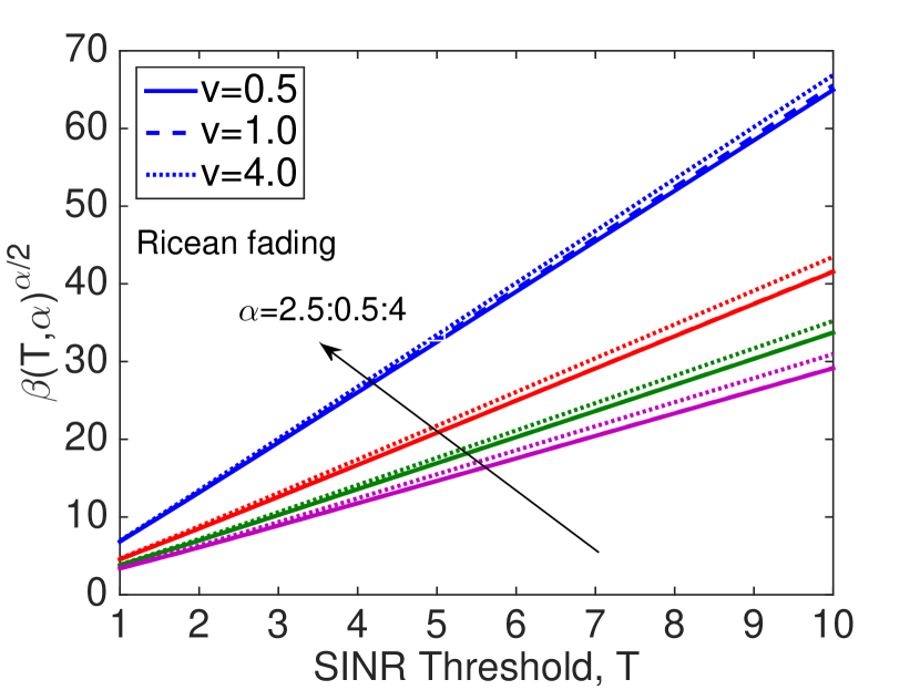
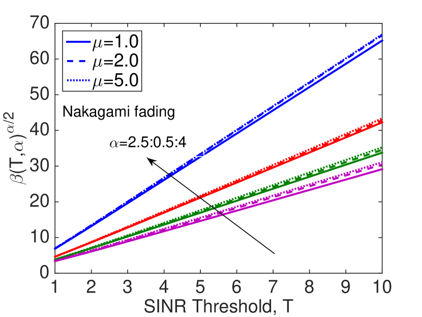
Separability of coverage distribution. For Rayleigh, Ricean and Nakagami small-scale fading distributions, the function β​(T,Ξ±)Ξ±/2𝛽superscriptT𝛼𝛼2\beta({\rm T},\alpha)^{\alpha/2} can be approximated as a linear function of TT\rm T as shown in Fig. 4. This relation555Although the expression β​(T,Ξ±)Ξ±/2/T𝛽superscriptT𝛼𝛼2T\beta({\rm T},\alpha)^{\alpha/2}/\rm T is not analytically tractable, we can approximate β​(T,Ξ±)Ξ±/2𝛽superscriptT𝛼𝛼2\beta({\rm T},\alpha)^{\alpha/2} as a linear function of TT\rm T because the lower incomplete Gamma function has light-tailed characteristics. Since the channel power distribution -which is exponential due to Rayleigh fading- is also light tailed, we can expect to observe such a linear approximation in our numerical results. greatly simplifies the analysis of the optimization problem given in (7).

Lemma 6.

Arbitrary Noise, Ξ±>2𝛼2\alpha>2. For arbitrary noise, from Assumption 1, the optimal caching distribution pc​(β‹…)subscript𝑝𝑐⋅p_{c}(\cdot) can be approximated as a Zipf distribution given by

pc​(i)β‰ˆ1iΞ³c/βˆ‘j=1M1jΞ³c,i=1,…,M,formulae-sequencesubscript𝑝𝑐𝑖1superscript𝑖subscript𝛾𝑐superscriptsubscript𝑗1𝑀1superscript𝑗subscript𝛾𝑐𝑖1…𝑀\displaystyle p_{c}(i)\approx{\frac{1}{i^{\gamma_{c}}}}\Big{/}{\sum\limits_{j=1}^{M}{\frac{1}{j^{\gamma_{c}}}}},\quad i=1,\ldots,M, (9)

where Ξ³c=Ξ³rΞ±/2+1<Ξ³r2subscript𝛾𝑐subscriptπ›Ύπ‘Ÿπ›Ό21subscriptπ›Ύπ‘Ÿ2\gamma_{c}=\frac{\gamma_{r}}{\alpha/2+1}<\frac{\gamma_{r}}{2} is the Zipf exponent for the caching pmf assuming Ξ±>2𝛼2\alpha>2.

Proof.

See Appendix -F. ∎

Interestingly, this result is the same as Rayleigh fading with small but non-zero noise model developed in Sect. IV-B, which follows from the monotonic transformation [32] caused by increasing the noise power Οƒ2superscript𝜎2\sigma^{2} in (6). According to the pmf given in (9), the optimal caching strategy exhibits less locality of reference than the input stream of requests. Therefore, it is a good caching strategy, which will be further verified in Sect. VII. Lemma 6 suggests that files with higher popularity should be cached less frequently than the demand for this file, and unpopular files should be cached more frequently than the demand for the file. However, high popularity files should be still cached at more locations compared to the low popularity files. The path loss evens out the file popularities and the caching distribution should be more uniform compared to the request distribution. The sequential transmission model shows that for a Zipf request distribution with exponent Ξ³rsubscriptπ›Ύπ‘Ÿ\gamma_{r}, which is skewed towards the most popular files, the optimal caching pmf should be also Zipf distributed with the relation Ξ³c<Ξ³r2subscript𝛾𝑐subscriptπ›Ύπ‘Ÿ2\gamma_{c}<\frac{\gamma_{r}}{2} for Ξ±>2𝛼2\alpha>2, implying that the caching pmf is more uniform than the request pmf.

The next result generalizes Lemma 6 to any request distribution pr​(β‹…)subscriptπ‘π‘Ÿβ‹…p_{r}(\cdot) rather than the Zipf distribution, and is derived solving (29) in Appendix -F using the separability of coverage from Assumption 1.

Theorem 1.

For arbitrary noise, if the small-scale fading is Rayleigh, Nakagami or Ricean distributed, from Assumption 1, for a general request pmf, pr​(β‹…)subscriptπ‘π‘Ÿβ‹…p_{r}(\cdot), the optimal caching pmf is approximated as

pc​(i)β‰ˆpr​(i)1(Ξ±/2+1)/βˆ‘j=1Mpr​(j)1(Ξ±/2+1),i=1,…,M.formulae-sequencesubscript𝑝𝑐𝑖subscriptπ‘π‘Ÿsuperscript𝑖1𝛼21superscriptsubscript𝑗1𝑀subscriptπ‘π‘Ÿsuperscript𝑗1𝛼21𝑖1…𝑀\displaystyle p_{c}(i)\approx{p_{r}(i)^{\frac{1}{(\alpha/2+1)}}}\Big{/}{\sum\limits_{j=1}^{M}{p_{r}(j)^{\frac{1}{(\alpha/2+1)}}}},\quad i=1,\ldots,M. (10)

From (10), it is required to flatten the request pmf to optimize the caching performance. Examples include the case of uniform demands, where the optimal caching distribution should be also uniform, and Geometric(p𝑝p) request distribution, for which the caching distribution satisfies Geometric(qπ‘žq), where q=1βˆ’(1βˆ’p)1(Ξ±/2+1)π‘ž1superscript1𝑝1𝛼21q=1-(1-p)^{\frac{1}{(\alpha/2+1)}}. In the case of Zipf demands, we can derive the same result as in Lemma 6.
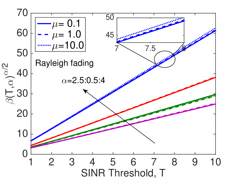
Refer to caption

(a) Rayleigh fading, param. ΞΌπœ‡\mu.

Refer to caption

(b) Ricean fading, distance param. v𝑣v.

Refer to caption

(c) Nakagami fading, shape param. ΞΌπœ‡\mu.

Figure 4: The linear relation between β​(T,Ξ±)Ξ±/2𝛽superscriptT𝛼𝛼2\beta({\rm T},\alpha)^{\alpha/2} and TT\rm T.
Lemma 7.

An Approximation for Arbitrary Noise with Ξ±=4𝛼4\alpha=4. For a total number of files M𝑀M and arbitrary noise with Ξ±=4𝛼4\alpha=4, the optimal caching pmf is

pc​(i)=ai+b​log⁑(i+1i),i=1,…,M,formulae-sequencesubscript𝑝𝑐𝑖subscriptπ‘Žπ‘–π‘π‘–1𝑖𝑖1…𝑀\displaystyle p_{c}(i)=a_{i}+b\log\Big{(}\frac{i+1}{i}\Big{)},\,\,i=1,\ldots,M, (11)

where b=μ​T​σ2​γrπ​λt​β​(T,4)π‘πœ‡Tsuperscript𝜎2subscriptπ›Ύπ‘Ÿπœ‹subscriptπœ†π‘‘π›½T4b=\frac{\sqrt{\mu\rm T\sigma^{2}}\gamma_{r}}{\pi\lambda_{t}\beta({\rm T},4)}, ai=1M+bMβ€‹βˆ‘j=1Mlog⁑(ji+1)subscriptπ‘Žπ‘–1𝑀𝑏𝑀superscriptsubscript𝑗1𝑀𝑗𝑖1a_{i}=\frac{1}{M}+\frac{b}{M}\sum\limits_{j=1}^{M}{\log\left(\frac{j}{i+1}\right)}, and the pmf is valid only if b≀[M​log⁑(M)βˆ’log⁑(M!)]βˆ’1𝑏superscriptdelimited-[]𝑀𝑀𝑀1b\leq[M\log(M)-\log(M!)]^{-1}.

Proof.

See Appendix -G. ∎

The distribution pc​(β‹…)subscript𝑝𝑐⋅p_{c}(\cdot) in (11) of Lemma 7 is a variety of Benford’s law [30], which is a special bounded case of Zipf’s law. Benford’s law refers to the frequency distribution of digits in many real-life sources of data and is characterized by the pmf FB​(i)=log10⁑(i+1i),i∈{1,…,9}formulae-sequencesubscript𝐹𝐡𝑖subscript10𝑖1𝑖𝑖1…9F_{B}(i)=\log_{10}\left(\frac{i+1}{i}\right),\,\,i\in\{1,\ldots,9\}. In distributed caching problems, the number of files, M𝑀M, is generally much greater than 9. Therefore, we generalize the law as FB​(i)=logM+1⁑(i+1i)subscript𝐹𝐡𝑖subscript𝑀1𝑖1𝑖F_{B}(i)=\log_{M+1}\left(\frac{i+1}{i}\right), i∈{1,…,M}𝑖1…𝑀i\in\{1,\ldots,M\}. The result in (11) has a very similar form as the Benford law with shift parameter aisubscriptπ‘Žπ‘–a_{i} for file i𝑖i and a scaling parameter b𝑏b, as determined in Lemma 7.

V A Lower and Upper Bound on the DSRDSR\rm{DSR} and Different Caching Strategies

The analysis of the DSRDSR\rm{DSR} becomes intractable for the multiple file case when the caching pdf does not have a simple form. Therefore, we derive a lower and upper bound to characterize the DSRDSR\rm{DSR} for the sequential serving model and provide two different caching strategies to maximize 𝖣𝖲𝖱𝖲subscript𝖣𝖲𝖱𝖲\sf{DSR_{S}}.

V-A Bounds on 𝖣𝖲𝖱𝖲subscript𝖣𝖲𝖱𝖲\sf{DSR_{S}}

We provide a lower and upper bound for 𝖣𝖲𝖱𝖲subscript𝖣𝖲𝖱𝖲\sf{DSR_{S}}, the DSRDSR\rm{DSR} of the sequential serving-based transmission model with multiple files. We discussed the optimal file caching problem for multiple file scenarios in [1]. Here, we compare our solution to the several bounds and other caching strategies.

V-A1 Upper Bound (UB)

Using the concavity of pcov​(T,Ξ»t​pc​(i),Ξ±)subscript𝑝covTsubscriptπœ†π‘‘subscript𝑝𝑐𝑖𝛼p_{\rm cov}({\rm T},\lambda_{t}p_{c}(i),\alpha) in pc​(i)subscript𝑝𝑐𝑖p_{c}(i), a UB is found as

βˆ‘i=1Mpr​(i)​pcov​(T,Ξ»t​pc​(i),Ξ±)​(a)<​pcov​(T,Ξ»tβ€‹βˆ‘i=1Mpr​(i)​pc​(i),Ξ±)​(b)≀​pcov​(T,Ξ»t​pr​(1),Ξ±),superscriptsubscript𝑖1𝑀subscriptπ‘π‘Ÿπ‘–subscript𝑝covTsubscriptπœ†π‘‘subscriptπ‘π‘π‘–π›Όπ‘Žsubscript𝑝covTsubscriptπœ†π‘‘superscriptsubscript𝑖1𝑀subscriptπ‘π‘Ÿπ‘–subscript𝑝𝑐𝑖𝛼𝑏subscript𝑝covTsubscriptπœ†π‘‘subscriptπ‘π‘Ÿ1𝛼\displaystyle\sum\nolimits_{i=1}^{M}{p_{r}(i)p_{\rm cov}({\rm T},\lambda_{t}p_{c}(i),\alpha)}\,\begin{subarray}{c}(a)\\ <\end{subarray}\,p_{\rm cov}\Big{(}{\rm T},\lambda_{t}\sum\nolimits_{i=1}^{M}{p_{r}(i)p_{c}(i)},\alpha\Big{)}\,\begin{subarray}{c}(b)\\ \leq\end{subarray}\,p_{\rm cov}({\rm T},\lambda_{t}p_{r}(1),\alpha), (12)

where (aπ‘Ža) follows from Jensen’s inequality, and (b𝑏b) follows from the assumption pr​(1)>pr​(i)subscriptπ‘π‘Ÿ1subscriptπ‘π‘Ÿπ‘–p_{r}(1)>p_{r}(i) for 1<i≀M1𝑖𝑀1<i\leq M that yields βˆ‘i=1Mpr​(i)​pc​(i)<pr​(1)β€‹βˆ‘i=1Mpc​(i)=pr​(1)superscriptsubscript𝑖1𝑀subscriptπ‘π‘Ÿπ‘–subscript𝑝𝑐𝑖subscriptπ‘π‘Ÿ1superscriptsubscript𝑖1𝑀subscript𝑝𝑐𝑖subscriptπ‘π‘Ÿ1\sum\nolimits_{i=1}^{M}{p_{r}(i)p_{c}(i)}<p_{r}(1)\sum\nolimits_{i=1}^{M}{p_{c}(i)}=p_{r}(1), where pr​(1)=(βˆ‘j=1Mjβˆ’Ξ³r)βˆ’1subscriptπ‘π‘Ÿ1superscriptsuperscriptsubscript𝑗1𝑀superscript𝑗subscriptπ›Ύπ‘Ÿ1p_{r}(1)=\Big{(}\sum\nolimits_{j=1}^{M}{j^{-\gamma_{r}}}\Big{)}^{-1}.

V-A2 Lower Bound (LB)

Using the fact that given pr​(β‹…)subscriptπ‘π‘Ÿβ‹…p_{r}(\cdot) is Zipf distributed, the optimal pc​(β‹…)subscript𝑝𝑐⋅p_{c}(\cdot) also has Zipf distribution as proven in Lemma 6 as a solution of the 𝖣𝖲𝖱𝖲subscript𝖣𝖲𝖱𝖲\sf{DSR_{S}} maximization problem in (7). As a result, any distribution that is not skewed towards the most popular files will yield a suboptimal 𝖣𝖲𝖱𝖲subscript𝖣𝖲𝖱𝖲\sf{DSR_{S}}. Hence a uniform caching distribution performs worse than the Zipf law, and a LB is found as

βˆ‘i=1Mpr​(i)​pcov​(T,Ξ»t​pc​(i),Ξ±)>βˆ‘i=1Mpr​(i)​pcov​(T,Ξ»tM,Ξ±)=pcov​(T,Ξ»tM,Ξ±).superscriptsubscript𝑖1𝑀subscriptπ‘π‘Ÿπ‘–subscript𝑝covTsubscriptπœ†π‘‘subscript𝑝𝑐𝑖𝛼superscriptsubscript𝑖1𝑀subscriptπ‘π‘Ÿπ‘–subscript𝑝covTsubscriptπœ†π‘‘π‘€π›Όsubscript𝑝covTsubscriptπœ†π‘‘π‘€π›Ό\displaystyle\sum\nolimits_{i=1}^{M}{p_{r}(i)p_{\rm cov}({\rm T},\lambda_{t}p_{c}(i),\alpha)}>\sum\nolimits_{i=1}^{M}{p_{r}(i)p_{\rm cov}\Big{(}{\rm T},\frac{\lambda_{t}}{M},\alpha\Big{)}}=p_{\rm cov}\Big{(}{\rm T},\frac{\lambda_{t}}{M},\alpha\Big{)}. (13)

V-B Caching Strategies for the Sequential Serving Model with Multiple Files

We propose two optimization formulations to maximize 𝖣𝖲𝖱𝖲subscript𝖣𝖲𝖱𝖲\sf{DSR_{S}} in the presence of multiple files, where the request and caching probabilities are known a priori because in general the optimal 𝖣𝖲𝖱𝖲subscript𝖣𝖲𝖱𝖲\sf{DSR_{S}} and the optimal caching distribution is not tractable. The first strategy, where we maximize the DSRDSR\rm{DSR} for the least popular file, favors the least desired file, i.e., the file with the lowest popularity, to prevent from fading away in the network. Therefore, we introduce the variables 0≀ρi≀10subscriptπœŒπ‘–10\leq\rho_{i}\leq 1 for files i∈{1,β‹―,M}𝑖1⋯𝑀i\in\{1,\cdots,M\} to weight the caching pmf pc​(β‹…)subscript𝑝𝑐⋅p_{c}(\cdot). The second strategy aims to maximize the DSRDSR\rm{DSR} of all files by optimizing the fraction ρisubscriptπœŒπ‘–\rho_{i}’s of the users for each file type. We assume the caching distribution is given. Then, we provide iterative techniques to solve the problems presented in this section.

V-B1 Maximum DSRDSR\rm{DSR} of the Least Desired File

Our motivation behind maximizing the DSRDSR\rm{DSR} of the least desired file is to prevent the files with low popularity from fading away in the network.

Lemma 8.

The caching probability of each file is weighted by ρi<1subscriptπœŒπ‘–1\rho_{i}<1 so that the total fraction of transmissions for all files, denoted by ΞΎπœ‰\xi satisfies ΞΎ=βˆ‘i=1Mρi​pc​(i)≀1πœ‰superscriptsubscript𝑖1𝑀subscriptπœŒπ‘–subscript𝑝𝑐𝑖1\xi=\sum\nolimits_{i=1}^{M}{\rho_{i}p_{c}(i)}\leq 1. Given Ξ·=maxi,ρi=1​pr​(i)​pc​(i)=pr​(j)​pc​(j)πœ‚π‘–subscriptπœŒπ‘–1subscriptπ‘π‘Ÿπ‘–subscript𝑝𝑐𝑖subscriptπ‘π‘Ÿπ‘—subscript𝑝𝑐𝑗\eta=\underset{i,\,\,\rho_{i}=1}{\max}\,\,{p_{r}(i)p_{c}(i)}=p_{r}(j)p_{c}(j) for some j𝑗j, the optimal solution is given by ρi=1{iβ‰₯j}+Ξ·pr​(i)​pc​(i)​1{1≀i<j}subscriptπœŒπ‘–subscript1π‘–π‘—πœ‚subscriptπ‘π‘Ÿπ‘–subscript𝑝𝑐𝑖subscript11𝑖𝑗\rho_{i}=1_{\{i\geq j\}}+\frac{\eta}{p_{r}(i)p_{c}(i)}1_{\{1\leq i<j\}}.

Proof.

See Appendix -H. ∎

V-B2 Maximum DSRDSR\rm{DSR} of All Files

We maximize the DSRDSR\rm{DSR} for all files without any prioritization.

Lemma 9.

The optimal solution to maximize the DSRDSR\rm{DSR} for all files is given by ρi=1subscriptπœŒπ‘–1\rho_{i}=1 for all i𝑖i.

Proof.

See Appendix -I. ∎

As well as maximizing the DSRDSR\rm{DSR} for the sequential model, one might wish to select a file with a particular request probability, and use π–£πŸ€π–£π–£πŸ€π–£\sf{D2D} to distribute this file and all files with higher probability or simultaneously cache all files using π–£πŸ€π–£π–£πŸ€π–£\sf{D2D} as detailed in Sect. VI. In the next section, we describe the simultaneous transmission of multiple files, and derive expressions for 𝖲𝖨𝖭𝖱𝖲𝖨𝖭𝖱\sf{SINR} distribution and DSRDSR\rm{DSR}.

VI Simultaneous Transmissions of Different Files with Arbitrary Noise

We consider the multiple file case, where a typical receiver requires a specific set of files, and the set of its transmitter candidates are the ones that contain any of the requested files. Each receiver gets the file from the closest transmitter candidate. The rest of the active transmitters that do not have the files requested are the interferers. We provide a detailed analysis for the 𝖲𝖨𝖭𝖱𝖲𝖨𝖭𝖱\sf{SINR} coverage next.

Assume that each receiver has a state, determined by the set of files it requests. For a receiver in state j𝑗j, the set of requested files is fr​(j)subscriptπ‘“π‘Ÿπ‘—f_{r}(j). Let the tagged receiver be y∈Φr𝑦subscriptΞ¦π‘Ÿy\in\Phi_{r} and in state j𝑗j, and Ξ¦t​(j)subscriptΦ𝑑𝑗\Phi_{t}(j) be the set of transmitters that a receiver in state j𝑗j can get data from. Hence, the set of transmitter candidates for user in state j𝑗j is the superposition given by Ξ¦t​(j)=βˆ‘i∈fr​(j)Ξ¦t,isubscriptΦ𝑑𝑗subscript𝑖subscriptπ‘“π‘Ÿπ‘—subscriptΦ𝑑𝑖\Phi_{t}(j)=\sum_{i\in f_{r}(j)}\Phi_{t,i}, where Ξ¦t,isubscriptΦ𝑑𝑖\Phi_{t,i} is the set of transmitters containing file i𝑖i. Let Ξ»jsubscriptπœ†π‘—\lambda_{j} be the density of Ξ¦t​(j)subscriptΦ𝑑𝑗\Phi_{t}(j), where Ξ»j=Ξ»t​pj=λ​γ1​pjsubscriptπœ†π‘—subscriptπœ†π‘‘subscriptπ‘π‘—πœ†subscript𝛾1subscript𝑝𝑗\lambda_{j}=\lambda_{t}p_{j}=\lambda\gamma_{1}p_{j}. The rest of the transmitters, i.e., βˆ‘iβˆ‰fr​(j)Ξ¦t,isubscript𝑖subscriptπ‘“π‘Ÿπ‘—subscriptΦ𝑑𝑖\sum_{i\notin f_{r}(j)}\Phi_{t,i}, is an independent process with density Ξ»tβˆ’Ξ»j=Ξ»t​(1βˆ’pj)=λ​γ1​(1βˆ’pj)subscriptπœ†π‘‘subscriptπœ†π‘—subscriptπœ†π‘‘1subscriptπ‘π‘—πœ†subscript𝛾11subscript𝑝𝑗\lambda_{t}-\lambda_{j}=\lambda_{t}(1-p_{j})=\lambda\gamma_{1}(1-p_{j}).

The sum pj=βˆ‘i∈fr​(j)pc​(i)subscript𝑝𝑗subscript𝑖subscriptπ‘“π‘Ÿπ‘—subscript𝑝𝑐𝑖p_{j}=\sum\nolimits_{i\in f_{r}(j)}p_{c}(i) gives the probability that the user has at least one of the files requested by any receiver in state j𝑗j. Hence, the density of the transmitter candidates Ξ»jsubscriptπœ†π‘—\lambda_{j} for a receiver in state j𝑗j are given by the product of λ​γ1πœ†subscript𝛾1\lambda\gamma_{1} and βˆ‘i∈fr​(j)pc​(i)subscript𝑖subscriptπ‘“π‘Ÿπ‘—subscript𝑝𝑐𝑖\sum\nolimits_{i\in f_{r}(j)}p_{c}(i), i.e., Ξ»j=Ξ»t​pj=λ​γ1β€‹βˆ‘i∈fr​(j)pc​(i)subscriptπœ†π‘—subscriptπœ†π‘‘subscriptπ‘π‘—πœ†subscript𝛾1subscript𝑖subscriptπ‘“π‘Ÿπ‘—subscript𝑝𝑐𝑖\lambda_{j}=\lambda_{t}p_{j}=\lambda\gamma_{1}\sum\nolimits_{i\in f_{r}(j)}p_{c}(i). Hence, using the nearest neighbor distribution of the typical receiver in state j𝑗j, the distance to its nearest transmitter is distributed as 𝖱𝖺𝗒𝗅𝖾𝗂𝗀𝗁​(Οƒj)∼rΟƒj2​exp⁑(βˆ’r22​σj2)similar-to𝖱𝖺𝗒𝗅𝖾𝗂𝗀𝗁subscriptπœŽπ‘—π‘ŸsuperscriptsubscriptπœŽπ‘—2superscriptπ‘Ÿ22superscriptsubscriptπœŽπ‘—2{\sf Rayleigh}(\sigma_{j})\sim\frac{r}{\sigma_{j}^{2}}\exp\Big{(}{-\frac{r^{2}}{2\sigma_{j}^{2}}}\Big{)}, for Οƒj=1/2​π​λjsubscriptπœŽπ‘—12πœ‹subscriptπœ†π‘—\sigma_{j}=1/\sqrt{2\pi\lambda_{j}} and rβ‰₯0π‘Ÿ0r\geq 0.

We assume that all users experience Rayleigh fading with mean 111, and constant transmit power of 1/ΞΌ1πœ‡1/\mu. Assuming user y𝑦y is at o, in state j𝑗j and is a receiver, and x is the tagged transmitter denoted by bosubscriptπ‘π‘œb_{o}, and the distance between them is rπ‘Ÿr, then the 𝖲𝖨𝖭𝖱𝖲𝖨𝖭𝖱\sf{SINR} at user y𝑦y is 𝖲𝖨𝖭𝖱j=h​rβˆ’Ξ±Οƒ2+Ir​(j)subscriptπ–²π–¨π–­π–±π‘—β„Žsuperscriptπ‘Ÿπ›Όsuperscript𝜎2subscriptπΌπ‘Ÿπ‘—{\sf{SINR}}_{j}=\frac{hr^{-\alpha}}{\sigma^{2}+I_{r(j)}}, where hβ„Žh is the channel gain parameter between xπ‘₯x and y𝑦y, Οƒ2superscript𝜎2\sigma^{2} is the white Gaussian noise, and Ir​(j)subscriptπΌπ‘Ÿπ‘—I_{r(j)} is the total interference at node y𝑦y in state j𝑗j, and given by the following expression: Ir​(j)=βˆ‘z∈Φt\bogz​rzβˆ’Ξ±=βˆ‘z∈Φt​(j)\bogz​rzβˆ’Ξ±+βˆ‘z∈Φt\Ξ¦t​(j)gz​rzβˆ’Ξ±subscriptπΌπ‘Ÿπ‘—subscript𝑧\subscriptΦ𝑑subscriptπ‘π‘œsubscript𝑔𝑧superscriptsubscriptπ‘Ÿπ‘§π›Όsubscript𝑧\subscriptΦ𝑑𝑗subscriptπ‘π‘œsubscript𝑔𝑧superscriptsubscriptπ‘Ÿπ‘§π›Όsubscript𝑧\subscriptΦ𝑑subscriptΦ𝑑𝑗subscript𝑔𝑧superscriptsubscriptπ‘Ÿπ‘§π›ΌI_{r(j)}=\sum\nolimits_{z\in\Phi_{t}\backslash b_{o}}{g_{z}r_{z}^{-\alpha}}=\sum\nolimits_{z\in\Phi_{t}(j)\backslash b_{o}}{g_{z}r_{z}^{-\alpha}}+\sum\nolimits_{z\in\Phi_{t}\backslash\Phi_{t}(j)}{g_{z}r_{z}^{-\alpha}}, where gzsubscript𝑔𝑧g_{z} is the channel gain from the interferer z𝑧z and the receiver y𝑦y, rzsubscriptπ‘Ÿπ‘§r_{z} is the interferer z𝑧z to receiver distance, on 𝖱𝖧𝖲𝖱𝖧𝖲\sf RHS, the first term is the interference due to the set of transmitters that has the files requested by the receiver, and the second term is the interference due to the rest of the transmitters that do not have any of the desired files by the receiver. The total interference depends on the transmission scheme. Compared to the nearest user association [27], it is hard to characterize the interference in dynamic caching models with different association techniques.

Theorem 2.

The probability of coverage of a typical user conditioned on being at state j𝑗j is given by666The definition of 𝒫cov​(T,Ξ»j,Ξ±)subscript𝒫covTsubscriptπœ†π‘—π›Ό\mathcal{P}_{\rm cov}({\rm T},\lambda_{j},\alpha) here is different from the definition of the classical downlink coverage probability pcov​(T,Ξ»,Ξ±)subscript𝑝covTπœ†π›Όp_{\rm cov}({\rm T},\lambda,\alpha) given in (1) due to the possibility of simultaneous transmissions of different file types.

𝒫cov​(T,Ξ»j,Ξ±)=π​λjβ€‹βˆ«0∞eβˆ’Ο€β€‹Ξ»j​v​(1βˆ’Ο2​(T,Ξ±))βˆ’Ο€β€‹Ξ»t​v​(ρ1​(T,Ξ±)+ρ2​(T,Ξ±))βˆ’T​σ2​vΞ±/2​dv,subscript𝒫covTsubscriptπœ†π‘—π›Όπœ‹subscriptπœ†π‘—superscriptsubscript0superscriptπ‘’πœ‹subscriptπœ†π‘—π‘£1subscript𝜌2Tπ›Όπœ‹subscriptπœ†π‘‘π‘£subscript𝜌1T𝛼subscript𝜌2T𝛼Tsuperscript𝜎2superscript𝑣𝛼2differential-d𝑣\displaystyle{\mathcal{P}_{\rm cov}({\rm T},\lambda_{j},\alpha)}=\pi\lambda_{j}\int\nolimits_{0}^{\infty}{e^{-\pi\lambda_{j}v(1-\rho_{2}({\rm T},\alpha))-\pi\lambda_{t}v(\rho_{1}({\rm T},\alpha)+\rho_{2}({\rm T},\alpha))-{\rm T}\sigma^{2}v^{\alpha/2}}\,\mathrm{d}v}, (14)

where ρ1​(T,Ξ±)=T2/Ξ±β€‹βˆ«Tβˆ’2/α∞11+uΞ±/2​dusubscript𝜌1T𝛼superscriptT2𝛼superscriptsubscriptsuperscriptT2𝛼11superscriptu𝛼2du\rho_{1}(\rm T,\alpha)={\rm T}^{2/\alpha}\int\nolimits_{{\rm T}^{-2/\alpha}}^{\infty}{\frac{1}{1+u^{\alpha/2}}\,\mathrm{d}u} and ρ2​(T,Ξ±)=T2/Ξ±β€‹βˆ«0Tβˆ’2/Ξ±11+uΞ±/2​dusubscript𝜌2T𝛼superscriptT2𝛼superscriptsubscript0superscriptT2𝛼11superscriptu𝛼2du\rho_{2}(\rm T,\alpha)={\rm T}^{2/\alpha}\int\nolimits_{0}^{{\rm T}^{-2/\alpha}}{\frac{1}{1+u^{\alpha/2}}\,\mathrm{d}u}.

Proof.

See Appendix -J. ∎

We now consider the special case of the path loss exponent Ξ±=4𝛼4\alpha=4, which is more tractable.

Corollary 3.

Letting H​(T,Ξ»t,pj)=(pjTβˆ’pj​tanβˆ’1⁑(1T)+Ο€2)​π​λt2​σ2𝐻Tsubscriptπœ†π‘‘subscript𝑝𝑗subscript𝑝𝑗Tsubscript𝑝𝑗superscript11Tπœ‹2πœ‹subscriptπœ†π‘‘2superscript𝜎2H({\rm T},\lambda_{t},p_{j})=\Big{(}\frac{p_{j}}{\sqrt{\rm T}}-p_{j}\tan^{-1}\left(\frac{1}{\sqrt{\rm T}}\right)+\frac{\pi}{2}\Big{)}\frac{\pi\lambda_{t}}{\sqrt{2\sigma^{2}}}, the probability of coverage of a typical user conditioned on being at state j𝑗j for the special case of Ξ±=4𝛼4\alpha=4 and ΞΌ=1πœ‡1\mu=1 is given by

𝒫cov​(T,Ξ»j,4)=π​λt​pj​πT​σ2​eH​(T,Ξ»t,pj)22​Q​(H​(T,Ξ»t,pj)).subscript𝒫covTsubscriptπœ†π‘—4πœ‹subscriptπœ†π‘‘subscriptπ‘π‘—πœ‹Tsuperscript𝜎2superscript𝑒𝐻superscriptTsubscriptπœ†π‘‘subscript𝑝𝑗22Q𝐻Tsubscriptπœ†π‘‘subscript𝑝𝑗\displaystyle{\mathcal{P}_{\rm cov}({\rm T},\lambda_{j},4)}=\pi\lambda_{t}p_{j}\sqrt{\frac{\pi}{\rm T\sigma^{2}}}e^{\frac{H({\rm T},\lambda_{t},p_{j})^{2}}{2}}{\rm Q}\big{(}H({\rm T},\lambda_{t},p_{j})\big{)}. (15)
Proof.

See Appendix -K. ∎

Since the term T​tanβˆ’1⁑(1T)Tsuperscript11T\sqrt{\rm T}\tan^{-1}\big{(}\frac{1}{\sqrt{\rm T}}\big{)} is increasing in TT\rm T and converges to 111 in the limit as TT\rm T goes to infinity, H​(T,Ξ»t,β‹…)𝐻Tsubscriptπœ†π‘‘β‹…H({\rm T},\lambda_{t},\cdot) is increasing in pjsubscript𝑝𝑗p_{j}, and positive. Furthermore, 𝒫cov​(T,Ξ»j,Ξ±)subscript𝒫covTsubscriptπœ†π‘—π›Ό\mathcal{P}_{\rm cov}({\rm T},\lambda_{j},\alpha) is monotonically increasing in pjsubscript𝑝𝑗p_{j}. This observation is essential in the characterization of the DSRDSR\rm{DSR} under different user criteria.

We consider two different strategies for the simultaneous transmission of multiple files, namely popularity-based and global models, which differ mainly in the set of files cached at the transmitters.

VI-A Popularity-based DSRDSR\rm{DSR}

In this approach, a set of files corresponding to the most popular ones in the network is cached simultaneously at all transmitters. We define 𝖣𝖲𝖱𝖯subscript𝖣𝖲𝖱𝖯\sf{DSR_{P}}, which stands for the DSRDSR\rm{DSR} of the popularity-based approach, and is calculated over the set of most popular files as

𝖣𝖲𝖱𝖯=λ​γ2β€‹βˆ‘kβˆˆπ’¦pr​(k)​𝒫cov​(T,ΞΎl,Ξ±),subscriptπ–£π–²π–±π–―πœ†subscript𝛾2subscriptπ‘˜π’¦subscriptπ‘π‘Ÿπ‘˜subscript𝒫covTsubscriptπœ‰π‘™π›Ό\displaystyle{\sf{DSR_{P}}}=\lambda\gamma_{2}\sum\nolimits_{k\in\mathcal{K}}p_{r}(k)\mathcal{P}_{\rm cov}({\rm T},\xi_{l},\alpha), (16)

where 𝒦𝒦\mathcal{K} is the set of the K𝐾K most popular files, and ΞΎl=λ​γ1β€‹βˆ‘iβˆˆβ„’pc​(i)subscriptπœ‰π‘™πœ†subscript𝛾1subscript𝑖ℒsubscript𝑝𝑐𝑖\xi_{l}=\lambda\gamma_{1}\sum\nolimits_{i\in\mathcal{L}}p_{c}(i), where β„’β„’\mathcal{L} is a set corresponding to the most popular K𝐾K files cached at the transmitters among the set of available files in the caches.

Consider the special case of (16), where only the most popular file in the network is cached at all the transmitters if available, i.e., |𝒦|=1𝒦1|\mathcal{K}|=1, which modifies (16) as 𝖣𝖲𝖱𝖯=λ​γ2​pr​(k)​𝒫cov​(T,λ​γ1​pc​(k),Ξ±)=(a)λ​γ2​pr​(k)​pcov​(T,λ​γ1​pc​(k),Ξ±)subscriptπ–£π–²π–±π–―πœ†subscript𝛾2subscriptπ‘π‘Ÿπ‘˜subscript𝒫covTπœ†subscript𝛾1subscriptπ‘π‘π‘˜π›Όsuperscriptπ‘Žπœ†subscript𝛾2subscriptπ‘π‘Ÿπ‘˜subscript𝑝covTπœ†subscript𝛾1subscriptπ‘π‘π‘˜π›Ό{\sf{DSR_{P}}}=\lambda\gamma_{2}p_{r}(k)\mathcal{P}_{\rm cov}({\rm T},\lambda\gamma_{1}p_{c}(k),\alpha)\stackrel{{\scriptstyle(a)}}{{=}}\lambda\gamma_{2}p_{r}(k)p_{\rm cov}({\rm T},\lambda\gamma_{1}p_{c}(k),\alpha), where (a)π‘Ž(a) follows from the fact that for |𝒦|=1𝒦1|\mathcal{K}|=1, the coverage probability becomes same as the sequential serving-based model in Sect. IV, and the most popular file index kπ‘˜k can be found from the demand distribution and is given by k=arg​maxi∈{1,…,M}​pr​(i)π‘˜π‘–1…𝑀argmaxsubscriptπ‘π‘Ÿπ‘–k=\underset{i\in\{1,\ldots,M\}}{\operatorname*{arg\,max}}\hskip 5.69046ptp_{r}(i), and hence the corresponding density of the transmitters is λ​γ1​pc​(k)πœ†subscript𝛾1subscriptπ‘π‘π‘˜\lambda\gamma_{1}p_{c}(k), where pr​(k)β‰₯pr​(l)subscriptπ‘π‘Ÿπ‘˜subscriptπ‘π‘Ÿπ‘™p_{r}(k)\geq p_{r}(l) for all l=1,…,M𝑙1…𝑀l=1,\ldots,M.

VI-B Global DSRDSR\rm{DSR}

Global DSRDSR\rm{DSR} is defined as the average performance of all users in the network, which is determined by the spatial characteristics of file distributions and the coverage of a typical user. The DSRDSR\rm{DSR} function in our model is state dependent since the coverage probability of a user is determined according to the files requested by the user. The expected global DSRDSR\rm{DSR} is given as follows:

𝖣𝖲𝖱𝖦=λ​γ2β€‹βˆ‘i=1Mpr​(i)​𝒫cov​(T,Ξ³1​λ​pc​(i),Ξ±).subscriptπ–£π–²π–±π–¦πœ†subscript𝛾2superscriptsubscript𝑖1𝑀subscriptπ‘π‘Ÿπ‘–subscript𝒫covTsubscript𝛾1πœ†subscript𝑝𝑐𝑖𝛼\displaystyle{\sf{DSR_{G}}}=\lambda\gamma_{2}\sum\nolimits_{i=1}^{M}{p_{r}(i)\mathcal{P}_{\rm cov}({\rm T},\gamma_{1}\lambda p_{c}(i),\alpha)}. (17)

A Discussion on the Various Transmission Models. Popularity-based transmission and global model in this section do not depend on the cache states. Instead, they both depend on the global file popularity distributions, and have similar characteristics as given in (16) and (17). It is intuitive to observe that the optimal caching distributions in both models follow similar trends as the request distribution. Sequential serving-based model in Sect. IV-A boils down to the scenario characterized in [27] where only a subset of transmitters and their candidate receivers are active simultaneously. Hence, this model mitigates interference and provides higher coverage than the other models. However, since the DSRDSR\rm{DSR} is a weighted function of the file transmit pmf pc​(β‹…)subscript𝑝𝑐⋅p_{c}(\cdot), the DSRDSR\rm{DSR} of the model is reduced.

Refer to caption
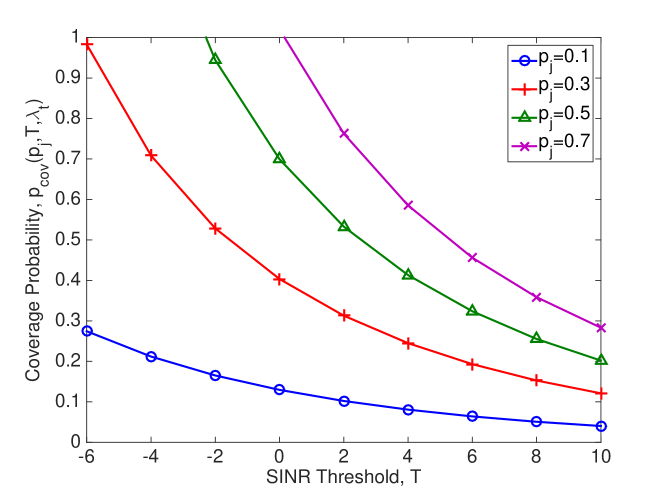
Figure 5: Analytical model for the 𝖲𝖨𝖭𝖱𝖲𝖨𝖭𝖱\sf{SINR} coverage probability for different transmitter densities where Ξ»=1πœ†1\lambda=1 and Ξ³1=0.4subscript𝛾10.4\gamma_{1}=0.4.
Refer to caption
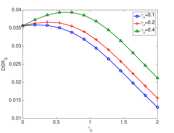
Figure 6: Average DSRDSR\rm{DSR} for the sequential model, 𝖣𝖲𝖱𝖲subscript𝖣𝖲𝖱𝖲\sf{DSR_{S}} versus Ξ³csubscript𝛾𝑐\gamma_{c} for Zipf request and Zipf caching distributions.
Refer to caption
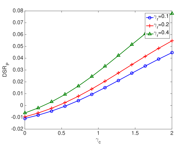
Figure 7: Average DSRDSR\rm{DSR} for the popularity-based model, 𝖣𝖲𝖱𝖯subscript𝖣𝖲𝖱𝖯\sf{DSR_{P}} versus Ξ³csubscript𝛾𝑐\gamma_{c} for Zipf request and Zipf caching distributions.
Refer to caption
Figure 8: Average DSRDSR\rm{DSR} for the global model, 𝖣𝖲𝖱𝖦subscript𝖣𝖲𝖱𝖦\sf{DSR_{G}} versus Ξ³csubscript𝛾𝑐\gamma_{c} for Zipf request and Zipf caching distributions.

Now, we present some numerical results on the general transmission models discussed and present results related to the popularity-based DSRDSR\rm{DSR}, global DSRDSR\rm{DSR} and sequential DSRDSR\rm{DSR}.

State dependent coverage probability. We illustrate the 𝖲𝖨𝖭𝖱𝖲𝖨𝖭𝖱\sf{SINR} coverage probability for varying pjsubscript𝑝𝑗p_{j} for a fixed fraction of transmitters (Ξ³1=0.4subscript𝛾10.4\gamma_{1}=0.4) in Fig. 6. The coverage probability is state dependent777The receiver’s state refers to the collection of files it requests. and for the receiver in state j𝑗j, the density of transmitters is given by Ξ»j=λ​pjsubscriptπœ†π‘—πœ†subscript𝑝𝑗\lambda_{j}=\lambda p_{j} where pj=Ξ³1β€‹βˆ‘i∈fr​(j)pc​(i)subscript𝑝𝑗subscript𝛾1subscript𝑖subscriptπ‘“π‘Ÿπ‘—subscript𝑝𝑐𝑖p_{j}=\gamma_{1}\sum\limits_{i\in f_{r}(j)}p_{c}(i). If the requested files are available in the set of transmitters, then the receiver has higher coverage. Therefore, for higher fraction of transmitters Ξ³1subscript𝛾1\gamma_{1}, the coverage probability is higher.

Caching performance of the proposed transmission models. The optimal caching strategies that maximize the caching problems of Sect. VI given in (16) and (17) are not necessarily Zipf distributed. However, without the Zipf distribution assumption, the optimization formulations become intractable since pcov​(T,Ξ»j,Ξ±)subscript𝑝covTsubscriptπœ†π‘—π›Όp_{\rm cov}({\rm T},\lambda_{j},\alpha) in (14) is nonlinear in the density of the users. Therefore, for simulation purposes, we find the optimal Zipf caching exponents that maximize the proposed functions.

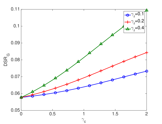
DSRDSR\rm{DSR} comparison. We investigate the variation of the sequential model 𝖣𝖲𝖱𝖲subscript𝖣𝖲𝖱𝖲\sf{DSR_{S}} with respect to the caching parameter Ξ³csubscript𝛾𝑐\gamma_{c}. From Fig. 6, we observe that Ξ³csubscript𝛾𝑐\gamma_{c} increases with the request distribution parameter Ξ³rsubscriptπ›Ύπ‘Ÿ\gamma_{r}, assuming both distributions are Zipf. In Figs. 8 and 8, we illustrate the variation of the popularity-based model 𝖣𝖲𝖱𝖯subscript𝖣𝖲𝖱𝖯\sf{DSR_{P}} and the global model 𝖣𝖲𝖱𝖦subscript𝖣𝖲𝖱𝖦\sf{DSR_{G}} with Ξ³csubscript𝛾𝑐\gamma_{c}. In both figures, it is clearly seen that as the requests become more skewed (higher Ξ³rsubscriptπ›Ύπ‘Ÿ\gamma_{r}), the DSRDSR\rm{DSR} increases. It also increases with Ξ³csubscript𝛾𝑐\gamma_{c}, which implies that the optimal caching distribution should also be skewed towards the highly popular files.

VII Numerical Results and Discussion

We evaluate the optimal caching distributions that maximize the DSRDSR\rm{DSR}. The simulation results are based on Sects. IV and V. We consider a general 𝖯𝖯𝖯𝖯𝖯𝖯\sf{PPP} network model with Rayleigh fading distribution with ΞΌ=1πœ‡1\mu=1 and Ξ±=4𝛼4\alpha=4 for small and general noise solutions. The requests are modeled by Zipf​(Ξ³r)Zipfsubscriptπ›Ύπ‘Ÿ\textrm{Zipf}(\gamma_{r}).

Refer to caption
Figure 9: For a Zipf​(Ξ³r)Zipfsubscriptπ›Ύπ‘Ÿ\textrm{Zipf}(\gamma_{r}) popularity distribution, Benford law and approximate Zipf​(Ξ³c)Zipfsubscript𝛾𝑐\textrm{Zipf}(\gamma_{c}) caching pmf for various M𝑀M.
Refer to caption
Figure 10: For a Zipf​(Ξ³r)Zipfsubscriptπ›Ύπ‘Ÿ\textrm{Zipf}(\gamma_{r}) popularity distribution, Benford law and optimal Zipf​(Ξ³c)Zipfsubscript𝛾𝑐\textrm{Zipf}(\gamma_{c}) pmf for different M𝑀M (𝖲𝖭𝖱=πŸ₯πŸ’π–²π–­π–±30\sf{SNR}=30 dB).

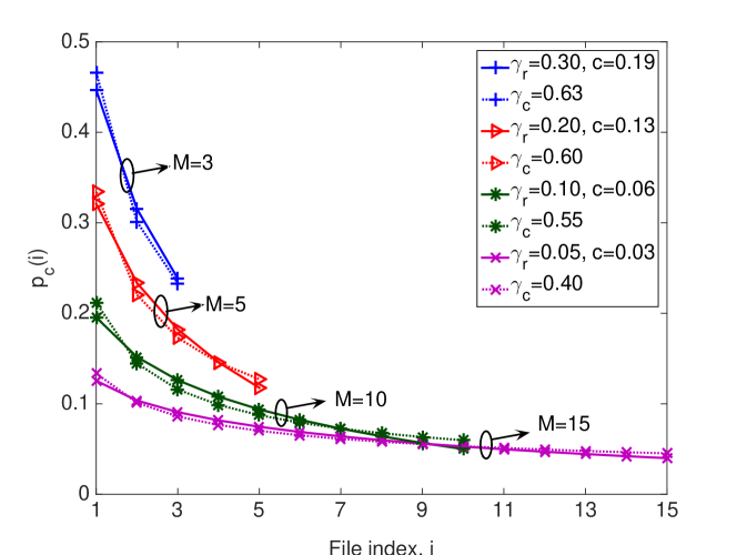
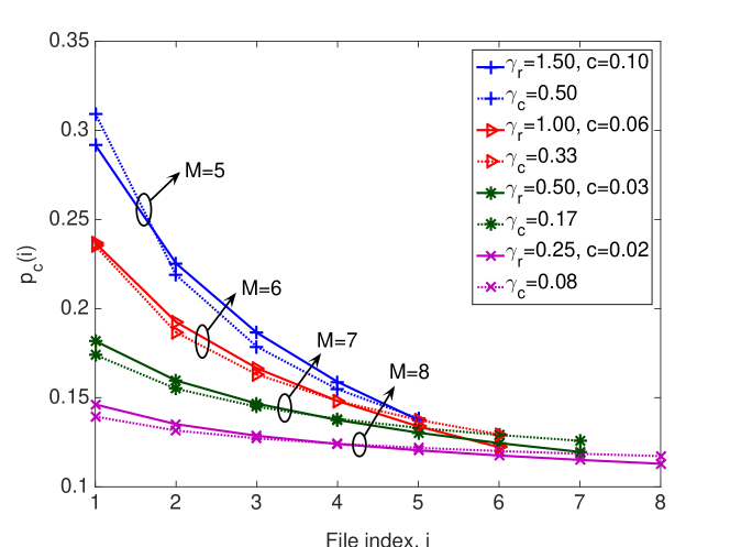
Benford versus Zipf distributions. In Figs. 10 and 10, we illustrate the trend of optimal Zipf caching distribution and the Benford law developed in Sect. IV for different numbers of total files. As seen from Fig. 10, these two distributions have similar characteristics. However, as Ξ³rsubscriptπ›Ύπ‘Ÿ\gamma_{r} increases, the range of M𝑀M for which Benford caching distribution in (11) and Zipf laws are comparable becomes narrower. For Ξ³r>0.3subscriptπ›Ύπ‘Ÿ0.3\gamma_{r}>0.3, it is not practical to approximate the Benford law with a Zipf distribution. In fact, as described in Sect. IV, as the noise level decreases, i.e., b=μ​T​σ2​γr/(π​λt​β​(T,4))π‘πœ‡Tsuperscript𝜎2subscriptπ›Ύπ‘Ÿπœ‹subscriptπœ†π‘‘π›½T4b={\sqrt{\mu\rm T\sigma^{2}}\gamma_{r}}/{(\pi\lambda_{t}\beta({\rm T},4))} drops, the optimal caching strategy converges to Zipf distribution. As seen in Fig. 10, for small noise, i.e., for high 𝖲𝖭𝖱𝖲𝖭𝖱\sf{SNR}, these laws behave similarly for relatively high Ξ³rsubscriptπ›Ύπ‘Ÿ\gamma_{r} values compared to the general noise case.

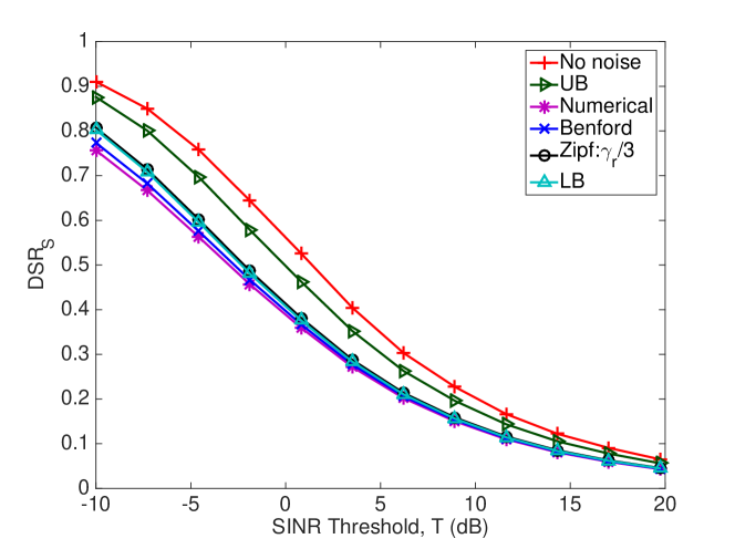
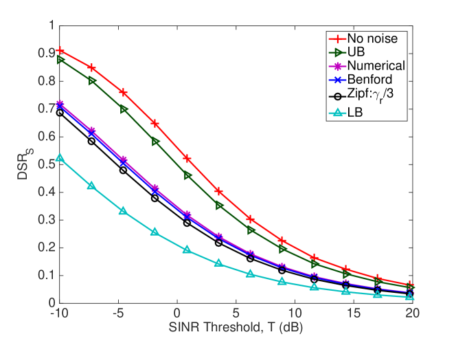
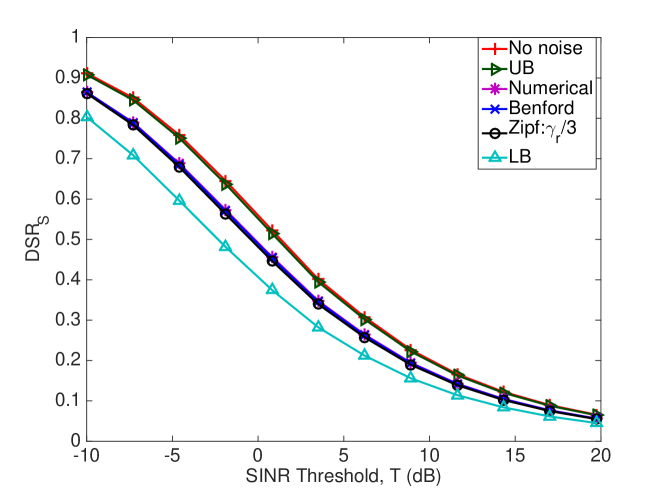
We now compare the DSRDSR\rm{DSR} of the sequential serving model for various Ξ³rsubscriptπ›Ύπ‘Ÿ\gamma_{r} based on the optimal solutions that are also Zipf distributed, as derived in Sect. IV, and the lower and upper bounds obtained in Sect. V. The numerical solutions are obtained by calculating the DSRDSR\rm{DSR} of various (random) caching distributions and picking the best one that achieves the highest DSRDSR\rm{DSR}.

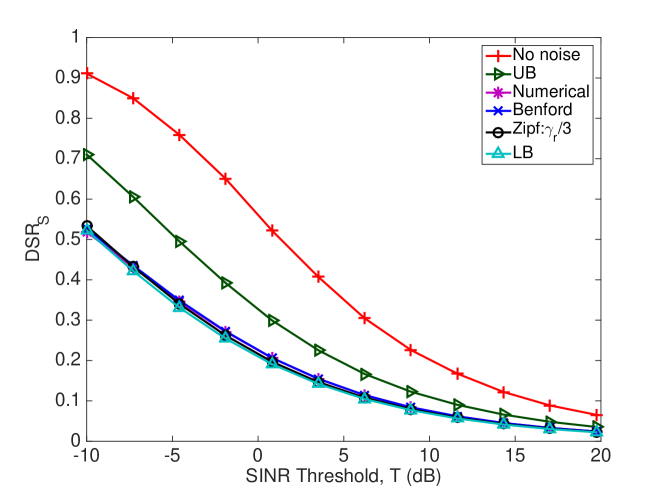
Zipf caching with Ξ³c=Ξ³r(Ξ±/2+1)subscript𝛾𝑐subscriptπ›Ύπ‘Ÿπ›Ό21\gamma_{c}=\frac{\gamma_{r}}{(\alpha/2+1)} is a good approximation to maximize the DSRDSR\rm{DSR}. In Fig. 12, we compare the performances of different caching strategies for a Zipf request distribution with parameter Ξ³r=0.5subscriptπ›Ύπ‘Ÿ0.5\gamma_{r}=0.5 and 𝖲𝖭𝖱=πŸ£π–²π–­π–±1\sf{SNR}=1. The Zipf caching distribution with parameter Ξ³r/3subscriptπ›Ύπ‘Ÿ3\gamma_{r}/3 is very close to the optimal solution evaluated numerically that is also very close to the simple lower bound derived in (13). Furthermore, Benford distribution has very similar characteristics as the optimal caching distribution solution. There is a huge gap between the UB and the no noise in terms of the DSRDSR\rm{DSR}, and the DSRDSR\rm{DSR} for the no noise case is the highest among all for all 𝖲𝖭𝖱𝖲𝖭𝖱\sf{SNR} or TT\rm T values.

Refer to caption
Figure 11: Bounds and approximations to the optimal 𝖣𝖲𝖱𝖲subscript𝖣𝖲𝖱𝖲\sf{DSR_{S}} for M=10𝑀10M=10, 𝖲𝖭𝖱=𝟣,Ξ»=𝟣formulae-sequence𝖲𝖭𝖱1πœ†1\sf{SNR}=1,\lambda=1, Zipf request pmf with Ξ³r=0.5subscriptπ›Ύπ‘Ÿ0.5\gamma_{r}=0.5.
Refer to caption
Figure 12: ​Bounds and approximations to the ​optimal ​𝖣𝖲𝖱𝖲subscript𝖣𝖲𝖱𝖲\sf{DSR_{S}} for M=10𝑀10M=10, 𝖲𝖭𝖱=𝟣𝟒,Ξ»=𝟣formulae-sequence𝖲𝖭𝖱10πœ†1\sf{SNR}=10,\lambda=1, Zipf request pmf with Ξ³r=0.5subscriptπ›Ύπ‘Ÿ0.5\gamma_{r}=0.5.
Refer to caption
Figure 13: Bounds and approximations to the optimal 𝖣𝖲𝖱𝖲subscript𝖣𝖲𝖱𝖲\sf{DSR_{S}} for M=10𝑀10M=10, 𝖲𝖭𝖱=𝟣,Ξ»=𝟣formulae-sequence𝖲𝖭𝖱1πœ†1\sf{SNR}=1,\lambda=1, Zipf request pmf with Ξ³r=2subscriptπ›Ύπ‘Ÿ2\gamma_{r}=2.
Refer to caption
Figure 14: Bounds and approximations to the ​optimal 𝖣𝖲𝖱𝖲subscript𝖣𝖲𝖱𝖲\sf{DSR_{S}} for M=10𝑀10M=10, 𝖲𝖭𝖱=𝟣𝟒,Ξ»=𝟣formulae-sequence𝖲𝖭𝖱10πœ†1\sf{SNR}=10,\lambda=1, Zipf request pmf with Ξ³r=2subscriptπ›Ύπ‘Ÿ2\gamma_{r}=2.

LB and UB get closer together as the 𝖲𝖭𝖱𝖲𝖭𝖱\sf{SNR} increases. In Fig. 12, we compare the performance of the caching distributions for a Zipf request pmf with parameter Ξ³r=0.5subscriptπ›Ύπ‘Ÿ0.5\gamma_{r}=0.5 and 𝖲𝖭𝖱=πŸ£πŸ’π–²π–­π–±10\sf{SNR}=10. At high 𝖲𝖭𝖱𝖲𝖭𝖱\sf{SNR}, the UB and LB are closer. Still, the numerical solution and the Zipf caching pmf with parameter Ξ³r/3subscriptπ›Ύπ‘Ÿ3\gamma_{r}/3 give similar densities of successful communication, which is very close to the lower bound because for that choice of Ξ³rsubscriptπ›Ύπ‘Ÿ\gamma_{r}, the request distribution converges to a uniform distribution. Benford caching distribution does not perform as well as the Zipf caching distribution, and is even worse than the LB. In Fig. 14, where Ξ³r=2subscriptπ›Ύπ‘Ÿ2\gamma_{r}=2 and 𝖲𝖭𝖱=πŸ£π–²π–­π–±1\sf{SNR}=1, the Zipf caching pmf with parameter Ξ³r/3subscriptπ›Ύπ‘Ÿ3\gamma_{r}/3 does not have the same performance as the optimal solution evaluated numerically. Benford distribution has also similar performance as the Zipf caching pmf. In Fig. 14, we also show that Zipf caching pmf and Benford distributions have similar performance as the numerical solution for Ξ³r=2subscriptπ›Ύπ‘Ÿ2\gamma_{r}=2 and 𝖲𝖭𝖱=πŸ£πŸ’π–²π–­π–±10\sf{SNR}=10.

Transmit Diversity. In the sequential serving model, where only one file is transmitted at a time network-wide, as discussed in Sect. IV, using a transmitter diversity scheme will improve the DSRDSR\rm{DSR}. For the second scenario presented in Sect. VI, in which different files are transmitted simultaneously, a similar diversity scheme can be applied instead of treating the other transmitters as interferers. Diversity combining techniques include the maximal-ratio combining (e.g., of the kπ‘˜k closest transmitters [25]), where the received signals are weighted with respect to their 𝖲𝖨𝖭𝖱𝖲𝖨𝖭𝖱\sf{SINR} and then summed, equal-gain combining, where all the received signals are summed coherently, i.e., the shot-noise model [31, Ch. 2], and the selection combining, which is based on the strongest π–£πŸ€π–£π–£πŸ€π–£\sf{D2D} user association, in which the received signal power (e.g., from the kπ‘˜k strongest users [25]) is considered.

Although diversity can decrease the outage probability, how to achieve this in practice is a critical issue. Diversity would seem to require synchronization of all transmitting devices at the physical layer unless higher layer coding is used, which might not be very practical for content distribution. Assuming full synchronization provides an upper bound on what could be achieved. Due to space constraints, we leave such analysis to future work.

VIII Conclusions

Content distribution using direct π–£πŸ€π–£π–£πŸ€π–£\sf{D2D} communications is a promising approach for optimizing the utilization of air-interface resources in 5G network. This work is the first attempt to derive closed form expressions for the optimal content caching distribution and the optimal caching strategies providing maximum DSRDSR\rm{DSR} in terms of the optimal fractions of transmitters and receivers in a π–£πŸ€π–£π–£πŸ€π–£\sf{D2D} network by using a homogeneous 𝖯𝖯𝖯𝖯𝖯𝖯\sf{PPP} model with realistic noise, interference and Rayleigh fading. We derive the 𝖲𝖨𝖭𝖱𝖲𝖨𝖭𝖱\sf{SINR} coverage for different transmission strategies in π–£πŸ€π–£π–£πŸ€π–£\sf{D2D} networks with some idealized modeling aspects, i.e., simultaneous scheduling of the users containing the same type of files and Zipf distributed content caching assumption for the general multi-file transmissions. Our results for the sequential transmission model show that the optimal caching pmf can also be modeled using the Zipf law and its exponent Ξ³csubscript𝛾𝑐\gamma_{c} is related to Ξ³rsubscriptπ›Ύπ‘Ÿ\gamma_{r} through a simple expression involving the path loss exponent: Ξ³c=Ξ³r(Ξ±/2+1)subscript𝛾𝑐subscriptπ›Ύπ‘Ÿπ›Ό21\gamma_{c}=\frac{\gamma_{r}}{(\alpha/2+1)}. The optimal content placement for more general demand profiles under Rayleigh, Ricean and Nakagami fading distributions suggests to flatten the request distribution to optimize the caching performance.

The limitations of the model can be overcome by investigating the optimal caching distributions that maximize the DSRDSR\rm{DSR} for the more general transmission settings incorporating the transmit diversity, and developing intelligent scheduling techniques, which are left as future work. The dynamic settings capturing the changes in the file popularities over time and the interference caused by simultaneous transmissions should also be considered. Future issues include the minimization of backhaul transmissions and 𝖑𝖲𝖑𝖲\sf{BS} overhead to optimize resource utilization through π–£πŸ€π–£π–£πŸ€π–£\sf{D2D} collaboration. Future work could also include the design of distributed caching strategies to maximize the hit probability for users by using an 𝖲𝖨𝖭𝖱𝖲𝖨𝖭𝖱\sf{SINR} coverage model or a distance-based coverage process given the limited range of π–£πŸ€π–£π–£πŸ€π–£\sf{D2D}.

-A Proof of Lemma 1

The problem in (3) is equivalent to π–£π–²π–±βˆ—=maxΞ³1<a≀1λ​(aβˆ’Ξ³11βˆ’Ξ³1)​𝖣𝖲𝖱T​(Ξ³1)superscript𝖣𝖲𝖱subscript𝛾1π‘Ž1πœ†π‘Žsubscript𝛾11subscript𝛾1subscript𝖣𝖲𝖱Tsubscript𝛾1{\sf{DSR}^{*}}=\underset{\gamma_{1}<a\leq 1}{\max}\quad\lambda\left(\frac{a-\gamma_{1}}{1-\gamma_{1}}\right){\sf{DSR}_{\rm T}}(\gamma_{1}), where 𝖣𝖲𝖱T​(Ξ³1)=Ξ³2​pcov​(T,λ​γ1,Ξ±)subscript𝖣𝖲𝖱Tsubscript𝛾1subscript𝛾2subscript𝑝covTπœ†subscript𝛾1𝛼{\sf{DSR}_{\rm T}}(\gamma_{1})=\gamma_{2}p_{\rm cov}({\rm T},\lambda\gamma_{1},\alpha) is the DSRDSR\rm{DSR} for a=1π‘Ž1a=1, and 𝖣𝖲𝖱T​(Ξ³1)subscript𝖣𝖲𝖱Tsubscript𝛾1{\sf{DSR}_{\rm T}}(\gamma_{1}) can be rewritten as 𝖣𝖲𝖱T​(Ξ³1)=(1βˆ’Ξ³1)​π​λ​γ1β€‹βˆ«0∞eβˆ’Ο€β€‹Ξ»β€‹Ξ³1​r​β​(T,Ξ±)βˆ’ΞΌβ€‹T​σ2​rΞ±2​drsubscript𝖣𝖲𝖱Tsubscript𝛾11subscript𝛾1πœ‹πœ†subscript𝛾1superscriptsubscript0superscriptπ‘’πœ‹πœ†subscript𝛾1π‘Ÿπ›½Tπ›Όπœ‡Tsuperscript𝜎2superscriptr𝛼2differential-dπ‘Ÿ{\sf{DSR}_{\rm T}}(\gamma_{1})=(1-\gamma_{1})\pi\lambda\gamma_{1}\int_{0}^{\infty}{e^{-\pi\lambda\gamma_{1}r\beta({\rm T},\alpha)-\mu\rm T\sigma^{2}r^{\frac{\alpha}{2}}}\,\mathrm{d}r}. Taking the derivative with respect to Ξ³1subscript𝛾1\gamma_{1}, we obtain

βˆ‚π–£π–²π–±T​(Ξ³1)βˆ‚Ξ³1+(aβˆ’1)(1βˆ’Ξ³1)​(aβˆ’Ξ³1)​𝖣𝖲𝖱T​(Ξ³1)=0.subscript𝖣𝖲𝖱Tsubscript𝛾1subscript𝛾1π‘Ž11subscript𝛾1π‘Žsubscript𝛾1subscript𝖣𝖲𝖱Tsubscript𝛾10\displaystyle\frac{\partial{\sf{DSR}_{\rm T}}(\gamma_{1})}{\partial\gamma_{1}}+\frac{(a-1)}{(1-\gamma_{1})(a-\gamma_{1})}{\sf{DSR}_{\rm T}}(\gamma_{1})=0. (18)

Using (1), the solution of (18) yields the following expression: 0<[1Ξ³1βˆ’1aβˆ’Ξ³1]π​λ​β​(T,Ξ±)=∫0∞eβˆ’Ο€β€‹Ξ»β€‹Ξ³1​r​β​(T,Ξ±)βˆ’ΞΌβ€‹T​σ2​rΞ±2​r​dr∫0∞eβˆ’Ο€β€‹Ξ»β€‹Ξ³1​r​β​(T,Ξ±)βˆ’ΞΌβ€‹T​σ2​rΞ±2​dr0delimited-[]1subscript𝛾11π‘Žsubscript𝛾1πœ‹πœ†π›½T𝛼superscriptsubscript0superscriptπ‘’πœ‹πœ†subscript𝛾1π‘Ÿπ›½Tπ›Όπœ‡Tsuperscript𝜎2superscriptr𝛼2π‘Ÿdifferential-dπ‘Ÿsuperscriptsubscript0superscriptπ‘’πœ‹πœ†subscript𝛾1π‘Ÿπ›½Tπ›Όπœ‡Tsuperscript𝜎2superscriptr𝛼2differential-dπ‘Ÿ0<\frac{\left[\frac{1}{\gamma_{1}}-\frac{1}{a-\gamma_{1}}\right]}{\pi\lambda\beta({\rm T},\alpha)}=\frac{\int_{0}^{\infty}{e^{-\pi\lambda\gamma_{1}r\beta({\rm T},\alpha)-\mu\rm T\sigma^{2}r^{\frac{\alpha}{2}}}r\,\mathrm{d}r}}{\int_{0}^{\infty}{e^{-\pi\lambda\gamma_{1}r\beta({\rm T},\alpha)-\mu\rm T\sigma^{2}r^{\frac{\alpha}{2}}}\,\mathrm{d}r}}. Thus, the positivity condition yields aβˆ’Ξ³1>Ξ³1π‘Žsubscript𝛾1subscript𝛾1a-\gamma_{1}>\gamma_{1}, implying Ξ³1<a/2subscript𝛾1π‘Ž2\gamma_{1}<a/2 and Ξ³2>a/2subscript𝛾2π‘Ž2\gamma_{2}>a/2.

-B Proof of Lemma 2

We use the relation ∫0∞eβˆ’(xβˆ’b)2​x​dx=12​eβˆ’b2+π​b​Q​(βˆ’2​b)superscriptsubscript0superscript𝑒superscriptπ‘₯𝑏2π‘₯differential-dπ‘₯12superscript𝑒superscript𝑏2πœ‹π‘Q2𝑏\int_{0}^{\infty}{\,e^{-(x-b)^{2}}x\mathrm{d}x}=\frac{1}{2}e^{-b^{2}}+\sqrt{\pi}b{\rm Q}(-\sqrt{2}b), which follows from a change of variables u=xβˆ’b𝑒π‘₯𝑏u=x-b and separating into two integrals, where Q​(x)=12β€‹Ο€β€‹βˆ«x∞eβˆ’y2/2​dyQπ‘₯12πœ‹superscriptsubscriptπ‘₯superscript𝑒superscript𝑦22differential-d𝑦{\rm Q}(x)=\frac{1}{\sqrt{2\pi}}\int_{x}^{\infty}{\,e^{-y^{2}/2}\mathrm{d}y} is the standard Gaussian tail probability. Using this relation, pcov​(T,λ​γ1,4)subscript𝑝covTπœ†subscript𝛾14p_{\rm cov}({\rm T},\lambda\gamma_{1},4) is given as

pcov​(T,λ​γ1,4)=π​λ​γ1β€‹βˆ«0∞eβˆ’Ο€β€‹Ξ»β€‹Ξ³1​r​β​(T,4)βˆ’ΞΌβ€‹T​σ2​r2​dr=Ο€32​λ​γ1μ​T​σ2​e(λ​γ1​π​β​(T,4))24​μ​T​σ2​Q​(λ​γ1​π​β​(T,4)2​μ​T​σ2).subscript𝑝covTπœ†subscript𝛾14πœ‹πœ†subscript𝛾1superscriptsubscript0superscriptπ‘’πœ‹πœ†subscript𝛾1π‘Ÿπ›½T4πœ‡Tsuperscript𝜎2superscriptr2differential-dπ‘Ÿsuperscriptπœ‹32πœ†subscript𝛾1πœ‡Tsuperscript𝜎2superscript𝑒superscriptπœ†subscript𝛾1πœ‹π›½T424πœ‡Tsuperscript𝜎2Qπœ†subscript𝛾1πœ‹π›½T42πœ‡Tsuperscript𝜎2\displaystyle p_{\rm cov}({\rm T},\lambda\gamma_{1},4)=\pi\lambda\gamma_{1}\int_{0}^{\infty}{e^{-\pi\lambda\gamma_{1}r\beta({\rm T},4)-\mu\rm T\sigma^{2}r^{2}}\,\mathrm{d}r}=\frac{\pi^{\frac{3}{2}}\lambda\gamma_{1}}{\sqrt{\mu\rm T\sigma^{2}}}e^{\frac{(\lambda\gamma_{1}\pi\beta({\rm T},4))^{2}}{4\mu\rm T\sigma^{2}}}{\rm Q}\Big{(}\frac{\lambda\gamma_{1}\pi\beta({\rm T},4)}{\sqrt{2\mu\rm T\sigma^{2}}}\Big{)}. (19)

The solution of (18) in Appendix -A for Ξ±=4𝛼4\alpha=4 yields the following expression:

[1Ξ³1βˆ’1aβˆ’Ξ³1]π​λ​β​(T,4)=eμ​T​σ2​u02β€‹βˆ«0∞eβˆ’ΞΌβ€‹T​σ2​(r+u0)2​r​dreμ​T​σ2​u02β€‹βˆ«0∞eβˆ’ΞΌβ€‹T​σ2​(r+u0)2​dr=(a)∫u0∞eβˆ’ΞΌβ€‹T​σ2​u2​u​duβˆ’u0β€‹βˆ«u0∞eβˆ’ΞΌβ€‹T​σ2​u2​du∫u0∞eβˆ’ΞΌβ€‹T​σ2​u2​dudelimited-[]1subscript𝛾11π‘Žsubscript𝛾1πœ‹πœ†π›½T4superscriptπ‘’πœ‡π‘‡superscript𝜎2superscriptsubscript𝑒02superscriptsubscript0superscriptπ‘’πœ‡Tsuperscript𝜎2superscriptrsubscriptu02π‘Ÿdifferential-dπ‘Ÿsuperscriptπ‘’πœ‡π‘‡superscript𝜎2superscriptsubscript𝑒02superscriptsubscript0superscriptπ‘’πœ‡Tsuperscript𝜎2superscriptrsubscriptu02differential-dπ‘Ÿsuperscriptπ‘Žsuperscriptsubscriptsubscript𝑒0superscriptπ‘’πœ‡Tsuperscript𝜎2superscriptu2𝑒differential-d𝑒subscript𝑒0superscriptsubscriptsubscript𝑒0superscriptπ‘’πœ‡Tsuperscript𝜎2superscriptu2differential-d𝑒superscriptsubscriptsubscript𝑒0superscriptπ‘’πœ‡Tsuperscript𝜎2superscriptu2differential-d𝑒\displaystyle\frac{\left[\frac{1}{\gamma_{1}}-\frac{1}{a-\gamma_{1}}\right]}{\pi\lambda\beta({\rm T},4)}=\frac{e^{\mu T\sigma^{2}u_{0}^{2}}\int_{0}^{\infty}{e^{-\mu\rm T\sigma^{2}\left(r+u_{0}\right)^{2}}r\,\mathrm{d}r}}{e^{\mu T\sigma^{2}u_{0}^{2}}\int_{0}^{\infty}{e^{-\mu\rm T\sigma^{2}\left(r+u_{0}\right)^{2}}\,\mathrm{d}r}}\,\stackrel{{\scriptstyle(a)}}{{=}}\,\frac{\int_{u_{0}}^{\infty}{e^{-\mu\rm T\sigma^{2}u^{2}}u\,\mathrm{d}u}-u_{0}\int_{u_{0}}^{\infty}{e^{-\mu\rm T\sigma^{2}u^{2}}\,\mathrm{d}u}}{\int_{u_{0}}^{\infty}{e^{-\mu\rm T\sigma^{2}u^{2}}\,\mathrm{d}u}}
=(b)12​μ​T​σ2β€‹βˆ«ΞΌβ€‹T​σ2​u02∞eβˆ’v1​dv1βˆ’Ο€β€‹Ξ»β€‹Ξ³1​β​(T,4)2​(μ​T​σ2)1.5β€‹βˆ«ΞΌβ€‹T​σ2​u0∞eβˆ’v22​dv21μ​T​σ2β€‹βˆ«ΞΌβ€‹T​σ2​u0∞eβˆ’v22​dv2=(c)π​λ​γ12​μ​T​σ2​[pcov​(T,λ​γ1,4)βˆ’1βˆ’Ξ²β€‹(T,4)],superscript𝑏absent12πœ‡Tsuperscript𝜎2superscriptsubscriptπœ‡Tsuperscript𝜎2superscriptsubscriptu02superscript𝑒subscript𝑣1differential-dsubscript𝑣1πœ‹πœ†subscript𝛾1𝛽T42superscriptπœ‡Tsuperscript𝜎21.5superscriptsubscriptπœ‡Tsuperscript𝜎2subscript𝑒0superscript𝑒superscriptsubscript𝑣22differential-dsubscript𝑣21πœ‡Tsuperscript𝜎2superscriptsubscriptπœ‡Tsuperscript𝜎2subscript𝑒0superscript𝑒superscriptsubscript𝑣22differential-dsubscript𝑣2superscriptπ‘πœ‹πœ†subscript𝛾12πœ‡Tsuperscript𝜎2delimited-[]subscript𝑝covsuperscriptTπœ†subscript𝛾141𝛽T4\displaystyle\stackrel{{\scriptstyle(b)}}{{=}}\frac{\frac{1}{2\mu\rm T\sigma^{2}}\int_{\mu\rm T\sigma^{2}u_{0}^{2}}^{\infty}{e^{-v_{1}}\,\mathrm{d}v_{1}}-\frac{\pi\lambda\gamma_{1}\beta({\rm T},4)}{2(\mu\rm T\sigma^{2})^{1.5}}\int_{\sqrt{\mu\rm T\sigma^{2}}u_{0}}^{\infty}{e^{-v_{2}^{2}}\,\mathrm{d}v_{2}}}{\frac{1}{\sqrt{\mu\rm T\sigma^{2}}}\int_{\sqrt{\mu\rm T\sigma^{2}}u_{0}}^{\infty}{e^{-v_{2}^{2}}\,\mathrm{d}v_{2}}}\stackrel{{\scriptstyle(c)}}{{=}}\,\frac{\pi\lambda\gamma_{1}}{2\mu\rm T\sigma^{2}}\left[p_{\rm cov}({\rm T},\lambda\gamma_{1},4)^{-1}-\beta({\rm T},4)\right], (20)

where u0=π​λ​γ1​β​(T,4)2​μ​T​σ2subscript𝑒0πœ‹πœ†subscript𝛾1𝛽T42πœ‡Tsuperscript𝜎2u_{0}=\frac{\pi\lambda\gamma_{1}\beta({\rm T},4)}{2\mu\rm T\sigma^{2}}, (a)π‘Ž(a) follows from employing a change of variables u=r+π​λ​γ1​β​(T,4)2​μ​T​σ2π‘’π‘Ÿπœ‹πœ†subscript𝛾1𝛽T42πœ‡Tsuperscript𝜎2u=r+\frac{\pi\lambda\gamma_{1}\beta({\rm T},4)}{2\mu\rm T\sigma^{2}}, (b)𝑏(b) also follows from employing change of variables v1=μ​T​σ2​u2subscript𝑣1πœ‡Tsuperscript𝜎2superscriptu2v_{1}=\mu\rm T\sigma^{2}u^{2} and v2=μ​T​σ2​usubscript𝑣2πœ‡Tsuperscript𝜎2𝑒v_{2}=\sqrt{\mu\rm T\sigma^{2}}u, and (c)𝑐(c) follows from employing the definition of standard Gaussian tail probability, and employing the definition of the coverage probability for Rayleigh fading, noise and Ξ±=4𝛼4\alpha=4 [27].

The relation in (-B) can be rearranged to obtain the following equality:

1Ξ³1​[1Ξ³1βˆ’1aβˆ’Ξ³1]=(π​λ)2​β​(T,4)22​μ​T​σ2​[β​(T,4)βˆ’1pcov​(T,λ​γ1,4)βˆ’1]​(a)>​ 0,1subscript𝛾1delimited-[]1subscript𝛾11π‘Žsubscript𝛾1superscriptπœ‹πœ†2𝛽superscriptT422πœ‡Tsuperscript𝜎2delimited-[]𝛽superscriptT41subscript𝑝covTπœ†subscript𝛾141π‘Žβ€‰0\displaystyle\frac{1}{\gamma_{1}}\left[\frac{1}{\gamma_{1}}-\frac{1}{a-\gamma_{1}}\right]=\frac{(\pi\lambda)^{2}\beta({\rm T},4)^{2}}{{2\mu\rm T\sigma^{2}}}\left[\frac{\beta({\rm T},4)^{-1}}{p_{\rm cov}({\rm T},\lambda\gamma_{1},4)}-1\right]\begin{subarray}{c}(a)\\ >\end{subarray}\,0, (21)

where (aπ‘Ža) follows from the fact that pcov​(T,λ​γ1,4)≀β​(T,4)βˆ’1subscript𝑝covTπœ†subscript𝛾14𝛽superscriptT41p_{\rm cov}({\rm T},\lambda\gamma_{1},4)\leq\beta({\rm T},4)^{-1}, where β​(T,4)βˆ’1𝛽superscriptT41\beta({\rm T},4)^{-1} is the no noise coverage. Given that Ξ³1subscript𝛾1\gamma_{1} is optimal, i.e., it satisfies (21), the maximum of the DSRDSR\rm{DSR} pcov​(T,λ​γ1,4)subscript𝑝covTπœ†subscript𝛾14p_{\rm cov}({\rm T},\lambda\gamma_{1},4) is

pcov​(T,λ​γ1,4)=(1Ξ³1​[1Ξ³1βˆ’1aβˆ’Ξ³1]​2​μ​T​σ2(π​λ)2​β​(T,4)+β​(T,4))βˆ’1,subscript𝑝covTπœ†subscript𝛾14superscript1subscript𝛾1delimited-[]1subscript𝛾11π‘Žsubscript𝛾12πœ‡Tsuperscript𝜎2superscriptπœ‹πœ†2𝛽T4𝛽T41\displaystyle p_{\rm cov}({\rm T},\lambda\gamma_{1},4)=\left(\frac{1}{\gamma_{1}}\Big{[}\frac{1}{\gamma_{1}}-\frac{1}{a-\gamma_{1}}\Big{]}\frac{{2\mu\rm T\sigma^{2}}}{(\pi\lambda)^{2}\beta({\rm T},4)}+\beta({\rm T},4)\right)^{-1}, (22)

using which π–£π–²π–±βˆ—superscript𝖣𝖲𝖱{\sf{DSR}^{*}} can be obtained. Combining (22) with (19), the optimal value of Ξ³1subscript𝛾1\gamma_{1} is found.

-C Proof of Lemma 3

The problem is equivalent to the formulation π–£π–²π–±βˆ—=maxΞ³1​λ​(1βˆ’Ξ³1)​[1β​(T,Ξ±)βˆ’ΞΌβ€‹T​σ2​(λ​γ1​π)βˆ’Ξ±2β​(T,Ξ±)Ξ±2+1​Γ​(1+Ξ±2)+o​(Οƒ2)]superscript𝖣𝖲𝖱subscript𝛾1πœ†1subscript𝛾1delimited-[]1𝛽Tπ›Όπœ‡Tsuperscript𝜎2superscriptπœ†subscript𝛾1πœ‹π›Ό2𝛽superscriptT𝛼𝛼21Ξ“1𝛼2π‘œsuperscript𝜎2{\sf{DSR}^{*}}=\underset{\gamma_{1}}{\max}\,\lambda(1-\gamma_{1})\big{[}\frac{1}{\beta({\rm T},\alpha)}-\frac{\mu{\rm T}\sigma^{2}\left(\lambda\gamma_{1}\pi\right)^{-\frac{\alpha}{2}}}{{\beta({\rm T},\alpha)}^{\frac{\alpha}{2}+1}}\Gamma\left(1+\frac{\alpha}{2}\right)+o\left(\sigma^{2}\right)\big{]}, which is concave in Ξ³1subscript𝛾1\gamma_{1}. Hence, taking its derivative with respect to Ξ³1subscript𝛾1\gamma_{1}, we obtain 1β​(T,Ξ±)+o​(Οƒ2)=μ​T​σ2​(λ​π)βˆ’Ξ±2β​(T,Ξ±)2Ξ±+1​Γ​(1+Ξ±2)​[Ξ±2​γ1βˆ’1+(1βˆ’Ξ±2)]​γ1βˆ’Ξ±21𝛽Tπ›Όπ‘œsuperscript𝜎2πœ‡Tsuperscript𝜎2superscriptπœ†πœ‹π›Ό2𝛽superscriptT𝛼2𝛼1Ξ“1𝛼2delimited-[]𝛼2superscriptsubscript𝛾111𝛼2superscriptsubscript𝛾1𝛼2\frac{1}{\beta({\rm T},\alpha)}+o\left(\sigma^{2}\right)=\frac{\mu\rm T\sigma^{2}(\lambda\pi)^{-\frac{\alpha}{2}}}{{\beta({\rm T},\alpha)}^{\frac{2}{\alpha}+1}}\Gamma\left(1+\frac{\alpha}{2}\right)\left[\frac{\alpha}{2}\gamma_{1}^{-1}+\left(1-\frac{\alpha}{2}\right)\right]\gamma_{1}^{-\frac{\alpha}{2}}. The solution Ξ³1βˆ—superscriptsubscript𝛾1\gamma_{1}^{*} satisfies the polynomial equation [2​β​(T,Ξ±)2Ξ±2βˆ’Ξ±β€‹(λ​π)Ξ±2μ​T​σ2​Γ​(1+Ξ±2)]​(Ξ³1βˆ—)Ξ±2+1​o​(Οƒ2)βˆ’Ξ³1βˆ—=Ξ±2βˆ’Ξ±delimited-[]2𝛽superscriptT𝛼2𝛼2𝛼superscriptπœ†πœ‹π›Ό2πœ‡Tsuperscript𝜎2Ξ“1𝛼2superscriptsuperscriptsubscript𝛾1𝛼21π‘œsuperscript𝜎2superscriptsubscript𝛾1𝛼2𝛼\big{[}\frac{2{\beta({\rm T},\alpha)}^{\frac{2}{\alpha}}}{2-\alpha}\frac{\left(\lambda\pi\right)^{\frac{\alpha}{2}}}{\mu\rm T\sigma^{2}\Gamma\left(1+\frac{\alpha}{2}\right)}\big{]}\left(\gamma_{1}^{*}\right)^{\frac{\alpha}{2}+1}o(\sigma^{2})-\gamma_{1}^{*}=\frac{\alpha}{2-\alpha}, using which π–£π–²π–±βˆ—superscript𝖣𝖲𝖱{\sf{DSR}^{*}} is found.

-D Proof of Lemma 4

Using (18), and letting Ξ±=4𝛼4\alpha=4, we have

[1Ξ³1βˆ’1aβˆ’Ξ³1]π​λ​β​(T,4)delimited-[]1subscript𝛾11π‘Žsubscript𝛾1πœ‹πœ†π›½T4\displaystyle\frac{\left[\frac{1}{\gamma_{1}}-\frac{1}{a-\gamma_{1}}\right]}{\pi\lambda\beta({\rm T},4)} =\displaystyle= ∫0∞eβˆ’Ο€β€‹Ξ»β€‹Ξ³1​r​β​(T,4)βˆ’ΞΌβ€‹T​σ2​r2​r​dr∫0∞eβˆ’Ο€β€‹Ξ»β€‹Ξ³1​r​β​(T,4)βˆ’ΞΌβ€‹T​σ2​r2​dr=(a)∫0∞eβˆ’Ο€β€‹Ξ»β€‹Ξ³1​r​β​(T,4)​(1βˆ’ΞΌβ€‹T​σ2​r2+o​(Οƒ2))​r​dr∫0∞eβˆ’Ο€β€‹Ξ»β€‹Ξ³1​r​β​(T,4)​(1βˆ’ΞΌβ€‹T​σ2​r2+o​(Οƒ2))​dr,superscriptπ‘Žsuperscriptsubscript0superscriptπ‘’πœ‹πœ†subscript𝛾1π‘Ÿπ›½T4πœ‡Tsuperscript𝜎2superscriptr2π‘Ÿdifferential-dπ‘Ÿsuperscriptsubscript0superscriptπ‘’πœ‹πœ†subscript𝛾1π‘Ÿπ›½T4πœ‡Tsuperscript𝜎2superscriptr2differential-dπ‘Ÿsuperscriptsubscript0superscriptπ‘’πœ‹πœ†subscript𝛾1π‘Ÿπ›½T41πœ‡Tsuperscript𝜎2superscriptr2osuperscript𝜎2rdrsuperscriptsubscript0superscriptπ‘’πœ‹πœ†subscript𝛾1π‘Ÿπ›½T41πœ‡Tsuperscript𝜎2superscriptr2osuperscript𝜎2dr\displaystyle\frac{\int_{0}^{\infty}{e^{-\pi\lambda\gamma_{1}r\beta({\rm T},4)-\mu\rm T\sigma^{2}r^{2}}r\,\mathrm{d}r}}{\int_{0}^{\infty}{e^{-\pi\lambda\gamma_{1}r\beta({\rm T},4)-\mu\rm T\sigma^{2}r^{2}}\,\mathrm{d}r}}\stackrel{{\scriptstyle(a)}}{{=}}\frac{\int_{0}^{\infty}{e^{-\pi\lambda\gamma_{1}r\beta({\rm T},4)}(1-\mu\rm T\sigma^{2}r^{2}+o(\sigma^{2}))r\,\mathrm{d}r}}{\int_{0}^{\infty}{e^{-\pi\lambda\gamma_{1}r\beta({\rm T},4)}(1-\mu\rm T\sigma^{2}r^{2}+o(\sigma^{2}))\,\mathrm{d}r}}, (23)
=\displaystyle= (π​λ​γ1​β​(T,4))2βˆ’6​(μ​T​σ2)+o​(Οƒ2)(π​λ​γ1​β​(T,4))3βˆ’2​(μ​T​σ2)​(π​λ​γ1​β​(T,4))+o​(Οƒ2),superscriptπœ‹πœ†subscript𝛾1𝛽T426πœ‡Tsuperscript𝜎2osuperscript𝜎2superscriptπœ‹πœ†subscript𝛾1𝛽T432πœ‡Tsuperscript𝜎2πœ‹πœ†subscript𝛾1𝛽T4osuperscript𝜎2\displaystyle\frac{(\pi\lambda\gamma_{1}\beta({\rm T},4))^{2}-6(\mu\rm T\sigma^{2})+o(\sigma^{2})}{{(\pi\lambda\gamma_{1}\beta({\rm T},4))}^{3}-2(\mu\rm T\sigma^{2})(\pi\lambda\gamma_{1}\beta({\rm T},4))+o(\sigma^{2})},

where (a)π‘Ž(a) follows from exp⁑(βˆ’x)=1βˆ’x+o​(x)π‘₯1π‘₯π‘œπ‘₯\exp(-x)=1-x+o(x) for xβ†’0β†’π‘₯0x\rightarrow 0. Then, using (23), we obtain

2​aΞ³1=(π​λ​β​(T,4))3​γ12+(μ​T​σ2)​(π​λ​β​(T,4))​2+o​(Οƒ2)(μ​T​σ2)​(π​λ​β​(T,4))​2+o​(Οƒ2)=(π​λ​γ1​β​(T,4))2+2​μ​T​σ2+o​(Οƒ2)2​μ​T​σ2+o​(Οƒ2).2π‘Žsubscript𝛾1superscriptπœ‹πœ†π›½T43superscriptsubscript𝛾12πœ‡Tsuperscript𝜎2πœ‹πœ†π›½T42osuperscript𝜎2πœ‡Tsuperscript𝜎2πœ‹πœ†π›½T42osuperscript𝜎2superscriptπœ‹πœ†subscript𝛾1𝛽T422πœ‡Tsuperscript𝜎2osuperscript𝜎22πœ‡Tsuperscript𝜎2osuperscript𝜎2\displaystyle\frac{2a}{\gamma_{1}}=\frac{(\pi\lambda\beta({\rm T},4))^{3}\gamma_{1}^{2}+(\mu\rm T\sigma^{2})(\pi\lambda\beta({\rm T},4))2+o(\sigma^{2})}{(\mu\rm T\sigma^{2})(\pi\lambda\beta({\rm T},4))2+o(\sigma^{2})}=\frac{(\pi\lambda\gamma_{1}\beta({\rm T},4))^{2}+2\mu\rm T\sigma^{2}+o(\sigma^{2})}{2\mu\rm T\sigma^{2}+o(\sigma^{2})}. (24)

Given that Ξ³1subscript𝛾1\gamma_{1} is optimal, i.e., it satisfies (24), pcov​(T,λ​γ1,4)subscript𝑝covTπœ†subscript𝛾14p_{\rm cov}({\rm T},\lambda\gamma_{1},4) is given by

pcov​(T,λ​γ1,4)=1β​(T,4)βˆ’2​μ​T​σ2​(λ​γ1​π)βˆ’2β​(T,4)3+o​(Οƒ2)=2β​(T,4)​[μ​T​σ2​(aβˆ’Ξ³1)+o​(Οƒ2)μ​T​σ2​(2​aβˆ’Ξ³1)+o​(Οƒ2)]+o​(Οƒ2),subscript𝑝covTπœ†subscript𝛾141𝛽T42πœ‡Tsuperscript𝜎2superscriptπœ†subscript𝛾1πœ‹2𝛽superscriptT43π‘œsuperscript𝜎22𝛽T4delimited-[]πœ‡Tsuperscript𝜎2asubscript𝛾1osuperscript𝜎2πœ‡Tsuperscript𝜎22asubscript𝛾1osuperscript𝜎2π‘œsuperscript𝜎2\displaystyle p_{\rm cov}({\rm T},\lambda\gamma_{1},4)=\frac{1}{\beta({\rm T},4)}-\frac{2\mu\rm T\sigma^{2}\left(\lambda\gamma_{1}\pi\right)^{-2}}{\beta({\rm T},4)^{3}}+o\left(\sigma^{2}\right)=\frac{2}{\beta({\rm T},4)}\left[\frac{\mu\rm T\sigma^{2}(a-\gamma_{1})+o(\sigma^{2})}{\mu\rm T\sigma^{2}(2a-\gamma_{1})+o(\sigma^{2})}\right]+o(\sigma^{2}),

using which the final result can be obtained. As Οƒ2β†’0β†’superscript𝜎20\sigma^{2}\to 0, limΟƒ2β†’0pcov​(T,λ​γ1,4)=2β​(T,4)​[aβˆ’Ξ³12​aβˆ’Ξ³1]β†’superscript𝜎20subscript𝑝covTπœ†subscript𝛾142𝛽T4delimited-[]π‘Žsubscript𝛾12π‘Žsubscript𝛾1\underset{\sigma^{2}\to 0}{\lim}\quad p_{\rm cov}({\rm T},\lambda\gamma_{1},4)=\frac{2}{\beta({\rm T},4)}\left[\frac{a-\gamma_{1}}{2a-\gamma_{1}}\right].

-E Proof of Lemma 5

For small but non-zero noise case, and given that βˆ‘i=1Mpc​(i)=1superscriptsubscript𝑖1𝑀subscript𝑝𝑐𝑖1\sum\nolimits_{i=1}^{M}p_{c}(i)=1, (7) can be rewritten as

maxpcsubscript𝑝𝑐\displaystyle\underset{p_{c}}{\max} λ​[1β​(T,Ξ±)+o​(Οƒ2)]βˆ’Ξ“β€‹(1+Ξ±2)​[μ​T​σ2​(λ​π)βˆ’Ξ±/2β​(T,Ξ±)Ξ±/2+1]β€‹βˆ‘i=1Mλ​pr​(i)​pc​(i)βˆ’Ξ±/2,πœ†delimited-[]1𝛽Tπ›Όπ‘œsuperscript𝜎2Ξ“1𝛼2delimited-[]πœ‡Tsuperscript𝜎2superscriptπœ†πœ‹π›Ό2𝛽superscriptT𝛼𝛼21superscriptsubscript𝑖1π‘€πœ†subscriptπ‘π‘Ÿπ‘–subscript𝑝𝑐superscript𝑖𝛼2\displaystyle\lambda\Big{[}\frac{1}{\beta({\rm T},\alpha)}+o\left(\sigma^{2}\right)\Big{]}-\Gamma\left(1+\frac{\alpha}{2}\right)\Big{[}\frac{\mu\rm T\sigma^{2}\left(\lambda\pi\right)^{-\alpha/2}}{\beta({\rm T},\alpha)^{\alpha/2+1}}\Big{]}\sum\limits_{i=1}^{M}{\lambda p_{r}(i)p_{c}(i)^{-\alpha/2}},

equivalent to minimizing βˆ‘i=1Mpr​(i)​pc​(i)βˆ’Ξ±2=(βˆ‘j=1M1jΞ³r)βˆ’1β€‹βˆ‘i=1Mpc​(i)βˆ’Ξ±2iΞ³rsuperscriptsubscript𝑖1𝑀subscriptπ‘π‘Ÿπ‘–subscript𝑝𝑐superscript𝑖𝛼2superscriptsuperscriptsubscript𝑗1𝑀1superscript𝑗subscriptπ›Ύπ‘Ÿ1superscriptsubscript𝑖1𝑀subscript𝑝𝑐superscript𝑖𝛼2superscript𝑖subscriptπ›Ύπ‘Ÿ\sum\nolimits_{i=1}^{M}{p_{r}(i)p_{c}(i)^{-\frac{\alpha}{2}}}=\big{(}\sum\nolimits_{j=1}^{M}{\frac{1}{j^{\gamma_{r}}}}\big{)}^{-1}\sum\nolimits_{i=1}^{M}{\frac{p_{c}(i)^{-\frac{\alpha}{2}}}{i^{\gamma_{r}}}} subject to βˆ‘i=1Mpc​(i)=1superscriptsubscript𝑖1𝑀subscript𝑝𝑐𝑖1\sum\nolimits_{i=1}^{M}p_{c}(i)=1.

Using the Lagrange multiplier method [33], we define, Λ​(𝐩𝐜,Ξ·)=βˆ‘i=1M1iΞ³r​pc​(i)βˆ’Ξ±/2+η​(βˆ‘i=1Mpc​(i)βˆ’1)Ξ›subscriptπ©πœπœ‚superscriptsubscript𝑖1𝑀1superscript𝑖subscriptπ›Ύπ‘Ÿsubscript𝑝𝑐superscript𝑖𝛼2πœ‚superscriptsubscript𝑖1𝑀subscript𝑝𝑐𝑖1\Lambda({\bf p_{c}},\eta)=\sum\limits_{i=1}^{M}{\frac{1}{i^{\gamma_{r}}}p_{c}(i)^{-\alpha/2}}+\eta\Big{(}\sum\limits_{i=1}^{M}{p_{c}(i)}-1\Big{)}, where 𝐩𝐜=[pc​(1)​…​pc​(M)]subscript𝐩𝐜delimited-[]subscript𝑝𝑐1…subscript𝑝𝑐𝑀{\bf p_{c}}=[p_{c}(1)\ldots p_{c}(M)], and Ξ·πœ‚\eta is the Lagrange multiplier. To maximize Λ​(𝐩𝐜,Ξ·)Ξ›subscriptπ©πœπœ‚\Lambda({\bf p_{c}},\eta), we take its partial derivatives with respect to 𝐩𝐜subscript𝐩𝐜{\bf p_{c}}. The partial derivative βˆ‚Ξ›β€‹(𝐩𝐜,Ξ·)βˆ‚Ξ·Ξ›subscriptπ©πœπœ‚πœ‚\frac{\partial\Lambda({\bf p_{c}},\eta)}{\partial\eta} reduces to the constraint equation.

Partial derivative of Λ​(𝐩𝐜,Ξ·)Ξ›subscriptπ©πœπœ‚\Lambda({\bf p_{c}},\eta) with respect to pc​(i)subscript𝑝𝑐𝑖p_{c}(i) gives (βˆ’Ξ±/2)​1iΞ³r​pc​(i)βˆ’Ξ±/2βˆ’1+Ξ·=0,i=1,…,Mformulae-sequence𝛼21superscript𝑖subscriptπ›Ύπ‘Ÿsubscript𝑝𝑐superscript𝑖𝛼21πœ‚0𝑖1…𝑀(-\alpha/2)\frac{1}{i^{\gamma_{r}}}p_{c}(i)^{-\alpha/2-1}+\eta=0,\quad i=1,\ldots,M. Hence, for any iβ‰ j𝑖𝑗i\neq j pair of file indices, we require (βˆ’Ξ±2)​1iΞ³r​pc​(i)βˆ’Ξ±2βˆ’1=(βˆ’Ξ±2)​1jΞ³r​pc​(j)βˆ’Ξ±2βˆ’1𝛼21superscript𝑖subscriptπ›Ύπ‘Ÿsubscript𝑝𝑐superscript𝑖𝛼21𝛼21superscript𝑗subscriptπ›Ύπ‘Ÿsubscript𝑝𝑐superscript𝑗𝛼21\big{(}-\frac{\alpha}{2}\big{)}\frac{1}{i^{\gamma_{r}}}p_{c}(i)^{-\frac{\alpha}{2}-1}=\big{(}-\frac{\alpha}{2}\big{)}\frac{1}{j^{\gamma_{r}}}p_{c}(j)^{-\frac{\alpha}{2}-1}, implying that pc​(j)/pc​(i)=(i/j)Ξ³rΞ±/2+1subscript𝑝𝑐𝑗subscript𝑝𝑐𝑖superscript𝑖𝑗subscriptπ›Ύπ‘Ÿπ›Ό21{p_{c}(j)}/{p_{c}(i)}=(i/j)^{\frac{\gamma_{r}}{\alpha/2+1}}. Then, pc​(i)subscript𝑝𝑐𝑖p_{c}(i) also has Zipf distribution with exponent Ξ³c=Ξ³rΞ±/2+1subscript𝛾𝑐subscriptπ›Ύπ‘Ÿπ›Ό21\gamma_{c}=\frac{\gamma_{r}}{\alpha/2+1}.

-F Proof of Lemma 6

We investigate the general solution of (7). Using the Lagrange multiplier method [33], we define Λ​(𝐩𝐜,Ξ·)=βˆ‘i=1MΞ»t​pr​(i)​pcov​(T,Ξ»t​pc​(i),Ξ±)+η​(βˆ‘i=1Mpc​(i)βˆ’1)Ξ›subscriptπ©πœπœ‚superscriptsubscript𝑖1𝑀subscriptπœ†π‘‘subscriptπ‘π‘Ÿπ‘–subscript𝑝covTsubscriptπœ†π‘‘subscriptπ‘π‘π‘–π›Όπœ‚superscriptsubscript𝑖1𝑀subscript𝑝𝑐𝑖1\Lambda({\bf p_{c}},\eta)=\sum\nolimits_{i=1}^{M}{\lambda_{t}p_{r}(i)p_{\rm cov}({\rm T},\lambda_{t}p_{c}(i),\alpha)}+\eta\Big{(}\sum\nolimits_{i=1}^{M}p_{c}(i)-1\Big{)}. The partial derivatives of Λ​(𝐩𝐜,Ξ·)Ξ›subscriptπ©πœπœ‚\Lambda({\bf p_{c}},\eta) with respect to pc​(i)subscript𝑝𝑐𝑖p_{c}(i) for i=1,…,M𝑖1…𝑀i=1,\ldots,M give M equations.

βˆ‚Ξ›β€‹(𝐩𝐜,Ξ·)βˆ‚pc​(i)Ξ›subscriptπ©πœπœ‚subscript𝑝𝑐𝑖\displaystyle\frac{\partial\Lambda({\bf p_{c}},\eta)}{\partial p_{c}(i)} =\displaystyle= Ξ»tpr(i)βˆ‚pcov​(T,Ξ»t​pc​(i),Ξ±)βˆ‚pc​(i)+Ξ·=Ξ»tpr(i)[πλt∫0∞eβˆ’Ο€β€‹Ξ»t​pc​(i)​r​β​(T,Ξ±)βˆ’ΞΌβ€‹T​σ2​rΞ±/2dr\displaystyle\lambda_{t}p_{r}(i)\frac{\partial p_{\rm cov}({\rm T},\lambda_{t}p_{c}(i),\alpha)}{\partial p_{c}(i)}+\eta=\lambda_{t}p_{r}(i)\Big{[}\pi\lambda_{t}\int\nolimits_{0}^{\infty}{e^{-\pi\lambda_{t}p_{c}(i)r\beta({\rm T},\alpha)-\mu{\rm T}\sigma^{2}r^{\alpha/2}}\,\mathrm{d}r} (25)
βˆ’\displaystyle- (πλt)2Ξ²(T,Ξ±)pc(i)∫0∞eβˆ’Ο€β€‹Ξ»t​pc​(i)​r​β​(T,Ξ±)βˆ’ΞΌβ€‹T​σ2​rΞ±/2rdr]+Ξ·.\displaystyle(\pi\lambda_{t})^{2}\beta({\rm T},\alpha)p_{c}(i)\int\nolimits_{0}^{\infty}{e^{-\pi\lambda_{t}p_{c}(i)r\beta({\rm T},\alpha)-\mu{\rm T}\sigma^{2}r^{\alpha/2}}r\,\mathrm{d}r}\Big{]}+\eta.

To maximize Λ​(𝐩𝐜,Ξ·)Ξ›subscriptπ©πœπœ‚\Lambda({\bf p_{c}},\eta), we equate the 𝖱𝖧𝖲𝖱𝖧𝖲\sf RHS of (25) to 0 and obtain

∫0∞[1βˆ’Ο€β€‹Ξ»t​β​(T,Ξ±)​pc​(i)​r]​eβˆ’Ο€β€‹Ξ»t​pc​(i)​r​β​(T,Ξ±)βˆ’ΞΌβ€‹T​σ2​rΞ±/2​dr=βˆ’Ξ·pr​(i)​π​λt2.superscriptsubscript0delimited-[]1πœ‹subscriptπœ†π‘‘π›½T𝛼subscriptπ‘π‘π‘–π‘Ÿsuperscriptπ‘’πœ‹subscriptπœ†π‘‘subscriptπ‘π‘π‘–π‘Ÿπ›½Tπ›Όπœ‡Tsuperscript𝜎2superscriptπ‘Ÿπ›Ό2differential-dπ‘Ÿπœ‚subscriptπ‘π‘Ÿπ‘–πœ‹superscriptsubscriptπœ†π‘‘2\displaystyle\int\nolimits_{0}^{\infty}{[1-\pi\lambda_{t}\beta({\rm T},\alpha)p_{c}(i)r]e^{-\pi\lambda_{t}p_{c}(i)r\beta({\rm T},\alpha)-\mu{\rm T}\sigma^{2}r^{\alpha/2}}\,\mathrm{d}r}=-\frac{\eta}{p_{r}(i)\pi\lambda_{t}^{2}}. (26)

The partial derivative of pcov​(T,Ξ»t​pc​(i),Ξ±)subscript𝑝covTsubscriptπœ†π‘‘subscript𝑝𝑐𝑖𝛼p_{\rm cov}({\rm T},\lambda_{t}p_{c}(i),\alpha) with respect to Ξ»tsubscriptπœ†π‘‘\lambda_{t} is given as

βˆ‚pcov​(T,Ξ»t​pc​(i),Ξ±)βˆ‚Ξ»t=π​pc​(i)β€‹βˆ«0∞eβˆ’Ο€β€‹Ξ»t​pc​(i)​r​β​(T,Ξ±)βˆ’ΞΌβ€‹T​σ2​rΞ±/2​drsubscript𝑝covTsubscriptπœ†π‘‘subscript𝑝𝑐𝑖𝛼subscriptπœ†π‘‘πœ‹subscript𝑝𝑐𝑖superscriptsubscript0superscriptπ‘’πœ‹subscriptπœ†π‘‘subscriptπ‘π‘π‘–π‘Ÿπ›½Tπ›Όπœ‡Tsuperscript𝜎2superscriptπ‘Ÿπ›Ό2differential-dπ‘Ÿ\displaystyle\frac{\partial{p_{\rm cov}}({\rm T},\lambda_{t}p_{c}(i),\alpha)}{\partial\lambda_{t}}=\pi p_{c}(i)\int\nolimits_{0}^{\infty}{e^{-\pi\lambda_{t}p_{c}(i)r\beta({\rm T},\alpha)-\mu{\rm T}\sigma^{2}r^{\alpha/2}}\,\mathrm{d}r} (27)
βˆ’(π​pc​(i))2​β​(T,Ξ±)​λtβ€‹βˆ«0∞eβˆ’Ο€β€‹Ξ»t​pc​(i)​r​β​(T,Ξ±)βˆ’ΞΌβ€‹T​σ2​rΞ±/2​r​dr=pc​(i)Ξ»tβ€‹βˆ‚pcov​(T,Ξ»t​pc​(i),Ξ±)βˆ‚pc​(i).superscriptπœ‹subscript𝑝𝑐𝑖2𝛽T𝛼subscriptπœ†π‘‘superscriptsubscript0superscriptπ‘’πœ‹subscriptπœ†π‘‘subscriptπ‘π‘π‘–π‘Ÿπ›½Tπ›Όπœ‡Tsuperscript𝜎2superscriptπ‘Ÿπ›Ό2π‘Ÿdifferential-dπ‘Ÿsubscript𝑝𝑐𝑖subscriptπœ†π‘‘subscript𝑝covTsubscriptπœ†π‘‘subscript𝑝𝑐𝑖𝛼subscript𝑝𝑐𝑖\displaystyle-(\pi p_{c}(i))^{2}\beta({\rm T},\alpha)\lambda_{t}\int\nolimits_{0}^{\infty}{e^{-\pi\lambda_{t}p_{c}(i)r\beta({\rm T},\alpha)-\mu{\rm T}\sigma^{2}r^{\alpha/2}}r\,\mathrm{d}r}=\frac{p_{c}(i)}{\lambda_{t}}\frac{\partial p_{\rm cov}({\rm T},\lambda_{t}p_{c}(i),\alpha)}{\partial p_{c}(i)}.

Combining the relations (26) and (27) results in βˆ‚pcov​(T,Ξ»t​pc​(i),Ξ±)βˆ‚Ξ»t=βˆ’Ξ·β€‹pc​(i)Ξ»t2​pr​(i)subscript𝑝covTsubscriptπœ†π‘‘subscript𝑝𝑐𝑖𝛼subscriptπœ†π‘‘πœ‚subscript𝑝𝑐𝑖superscriptsubscriptπœ†π‘‘2subscriptπ‘π‘Ÿπ‘–\frac{\partial p_{\rm cov}({\rm T},\lambda_{t}p_{c}(i),\alpha)}{\partial\lambda_{t}}=-\eta\frac{p_{c}(i)}{\lambda_{t}^{2}p_{r}(i)}. Using the definition of pcov​(T,Ξ»t​pc​(i),Ξ±)subscript𝑝covTsubscriptπœ†π‘‘subscript𝑝𝑐𝑖𝛼p_{\rm cov}({\rm T},\lambda_{t}p_{c}(i),\alpha), we can easily note that pcov​(T,Ξ»t​pc​(i),Ξ±)=pcov​(T​(pc​(j)/pc​(i))Ξ±/2,Ξ»t​pc​(j),Ξ±)subscript𝑝covTsubscriptπœ†π‘‘subscript𝑝𝑐𝑖𝛼subscript𝑝covTsuperscriptsubscript𝑝𝑐𝑗subscript𝑝𝑐𝑖𝛼2subscriptπœ†π‘‘subscript𝑝𝑐𝑗𝛼p_{\rm cov}({\rm T},\lambda_{t}p_{c}(i),\alpha)=p_{\rm cov}({\rm T}\left({p_{c}(j)}/{p_{c}(i)}\right)^{\alpha/2},\lambda_{t}p_{c}(j),\alpha). Taking the derivative of this expression with respect to Ξ»tsubscriptπœ†π‘‘\lambda_{t}, we have

βˆ‚pcov​(T,Ξ»t​pc​(j),Ξ±)βˆ‚Ξ»t=βˆ’Ξ·β€‹pc​(j)Ξ»t2​pr​(j)=βˆ‚pcov​(T,Ξ»t​pc​(i),Ξ±)βˆ‚Ξ»t​pr​(i)/pc​(i)pr​(j)/pc​(j).subscript𝑝covTsubscriptπœ†π‘‘subscript𝑝𝑐𝑗𝛼subscriptπœ†π‘‘πœ‚subscript𝑝𝑐𝑗superscriptsubscriptπœ†π‘‘2subscriptπ‘π‘Ÿπ‘—subscript𝑝covTsubscriptπœ†π‘‘subscript𝑝𝑐𝑖𝛼subscriptπœ†π‘‘subscriptπ‘π‘Ÿπ‘–subscript𝑝𝑐𝑖subscriptπ‘π‘Ÿπ‘—subscript𝑝𝑐𝑗\displaystyle\frac{\partial p_{\rm cov}({\rm T},\lambda_{t}p_{c}(j),\alpha)}{\partial\lambda_{t}}=-\eta\frac{p_{c}(j)}{\lambda_{t}^{2}p_{r}(j)}=\frac{\partial p_{\rm cov}({\rm T},\lambda_{t}p_{c}(i),\alpha)}{\partial\lambda_{t}}\frac{p_{r}(i)/p_{c}(i)}{p_{r}(j)/p_{c}(j)}. (28)

We can rewrite (28) using the expression for pcov​(T,Ξ»t​pc​(i),Ξ±)subscript𝑝covTsubscriptπœ†π‘‘subscript𝑝𝑐𝑖𝛼p_{\rm cov}({\rm T},\lambda_{t}p_{c}(i),\alpha) as follows

βˆ‚pcov​(T,Ξ»t​pc​(j),Ξ±)βˆ‚Ξ»t=βˆ‚pcov​(T​(pc​(j)pc​(i))Ξ±/2,Ξ»t​pc​(j),Ξ±)βˆ‚Ξ»t​pr​(i)/pc​(i)pr​(j)/pc​(j).subscript𝑝covTsubscriptπœ†π‘‘subscript𝑝𝑐𝑗𝛼subscriptπœ†π‘‘subscript𝑝covTsuperscriptsubscript𝑝𝑐𝑗subscript𝑝𝑐𝑖𝛼2subscriptπœ†π‘‘subscript𝑝𝑐𝑗𝛼subscriptπœ†π‘‘subscriptπ‘π‘Ÿπ‘–subscript𝑝𝑐𝑖subscriptπ‘π‘Ÿπ‘—subscript𝑝𝑐𝑗\displaystyle\frac{\partial p_{\rm cov}({\rm T},\lambda_{t}p_{c}(j),\alpha)}{\partial\lambda_{t}}=\frac{\partial p_{\rm cov}({\rm T}\left(\frac{p_{c}(j)}{p_{c}(i)}\right)^{\alpha/2},\lambda_{t}p_{c}(j),\alpha)}{\partial\lambda_{t}}\frac{p_{r}(i)/p_{c}(i)}{p_{r}(j)/p_{c}(j)}. (29)

Next, by employing a change of variables v=r​β​(T,Ξ±)π‘£π‘Ÿπ›½T𝛼v=r\beta({\rm T},\alpha), we can rewrite (1) in Definition 1 as

pcov​(T,Ξ»t,Ξ±)=π​λtβ​(T,Ξ±)β€‹βˆ«0∞eβˆ’Ο€β€‹Ξ»t​vβˆ’ΞΌβ€‹[Tβ​(T,Ξ±)Ξ±/2]​σ2​vΞ±/2​dv.subscript𝑝covTsubscriptπœ†π‘‘π›Όπœ‹subscriptπœ†π‘‘π›½T𝛼superscriptsubscript0superscriptπ‘’πœ‹subscriptπœ†π‘‘π‘£πœ‡delimited-[]T𝛽superscriptT𝛼𝛼2superscript𝜎2superscript𝑣𝛼2differential-d𝑣\displaystyle p_{\rm cov}({\rm T},\lambda_{t},\alpha)=\frac{\pi\lambda_{t}}{\beta({\rm T},\alpha)}\int\nolimits_{0}^{\infty}{e^{-\pi\lambda_{t}v-\mu\left[\frac{\rm T}{\beta({\rm T},\alpha)^{\alpha/2}}\right]\sigma^{2}v^{\alpha/2}}\,\mathrm{d}v}. (30)

We investigate the relation between β​(T,Ξ±)Ξ±/2𝛽superscriptT𝛼𝛼2\beta({\rm T},\alpha)^{\alpha/2} and TT\rm T in Fig. 4, for practical α𝛼\alpha and ΞΌπœ‡\mu values, and observe the linear dependence, where the slope is mainly determined by α𝛼\alpha, and changes only slightly by varying ΞΌπœ‡\mu. Based on these simulations, since β​(T,Ξ±)Ξ±/2/T𝛽superscriptT𝛼𝛼2T\beta({\rm T},\alpha)^{\alpha/2}/{\rm T} is invariant to TT\rm T and using the relation in (30), it is reasonable to write pcov​(T,Ξ»t​pc​(j),Ξ±)subscript𝑝covTsubscriptπœ†π‘‘subscript𝑝𝑐𝑗𝛼p_{\rm cov}({\rm T},\lambda_{t}p_{c}(j),\alpha) as a separable function which is the form f​(Ξ»t​pc​(j),Ξ±)​g​(T)𝑓subscriptπœ†π‘‘subscript𝑝𝑐𝑗𝛼𝑔Tf(\lambda_{t}p_{c}(j),\alpha)g({\rm T}). By taking its derivative with respect to Ξ»tsubscriptπœ†π‘‘\lambda_{t}, we can then rewrite (29) as g​(T)=g​(T​(pc​(j)pc​(i))Ξ±/2)​pc​(j)pc​(i)​(ji)Ξ³r𝑔T𝑔Tsuperscriptsubscript𝑝𝑐𝑗subscript𝑝𝑐𝑖𝛼2subscript𝑝𝑐𝑗subscript𝑝𝑐𝑖superscript𝑗𝑖subscriptπ›Ύπ‘Ÿg({\rm T})=g\Big{(}{\rm T}\Big{(}\frac{p_{c}(j)}{p_{c}(i)}\Big{)}^{\alpha/2}\Big{)}\frac{p_{c}(j)}{p_{c}(i)}\Big{(}\frac{j}{i}\Big{)}^{\gamma_{r}}. Taking the derivative of both sides with respect to TT\rm T, we obtain d​g​(T)d​T=(pc​(j)pc​(i))Ξ±/2​d​g​(T)d​T​pc​(j)pc​(i)​(ji)Ξ³r𝑑𝑔T𝑑Tsuperscriptsubscript𝑝𝑐𝑗subscript𝑝𝑐𝑖𝛼2𝑑𝑔T𝑑Tsubscript𝑝𝑐𝑗subscript𝑝𝑐𝑖superscript𝑗𝑖subscriptπ›Ύπ‘Ÿ\frac{dg({\rm T})}{d\rm T}=\Big{(}\frac{p_{c}(j)}{p_{c}(i)}\Big{)}^{\alpha/2}\frac{dg({\rm T})}{d\rm T}\frac{p_{c}(j)}{p_{c}(i)}\Big{(}\frac{j}{i}\Big{)}^{\gamma_{r}}, implying that pc​(j)/pc​(i)=(i/j)Ξ³rΞ±/2+1subscript𝑝𝑐𝑗subscript𝑝𝑐𝑖superscript𝑖𝑗subscriptπ›Ύπ‘Ÿπ›Ό21p_{c}(j)/p_{c}(i)=\left(i/j\right)^{\frac{\gamma_{r}}{\alpha/2+1}}. Then, pc​(β‹…)subscript𝑝𝑐⋅p_{c}(\cdot) is also Zipf(Ξ³csubscript𝛾𝑐\gamma_{c}) distributed with Ξ³c=Ξ³rΞ±/2+1subscript𝛾𝑐subscriptπ›Ύπ‘Ÿπ›Ό21\gamma_{c}=\frac{\gamma_{r}}{\alpha/2+1}.

-G Proof of Lemma 7

The coverage probability pcov​(T,Ξ»t​pc​(i),4)subscript𝑝covTsubscriptπœ†π‘‘subscript𝑝𝑐𝑖4p_{\rm cov}({\rm T},\lambda_{t}p_{c}(i),4) for Rayleigh fading and general noise with Ξ±=4𝛼4\alpha=4 is pcov​(T,Ξ»t​pc​(i),4)=Ο€1/2​2β​(T,4)​x​Q​(x)​exp⁑(x2/2)subscript𝑝covTsubscriptπœ†π‘‘subscript𝑝𝑐𝑖4superscriptπœ‹122𝛽T4π‘₯𝑄π‘₯superscriptπ‘₯22p_{\rm cov}({\rm T},\lambda_{t}p_{c}(i),4)=\frac{\pi^{1/2}\sqrt{2}}{\beta({\rm T},4)}xQ(x)\exp(x^{2}/2), where x=π​λt​pc​(i)​β​(T,4)2​μ​T​σ2π‘₯πœ‹subscriptπœ†π‘‘subscript𝑝𝑐𝑖𝛽T42πœ‡Tsuperscript𝜎2x=\frac{\pi\lambda_{t}p_{c}(i)\beta({\rm T},4)}{\sqrt{2\mu\rm T\sigma^{2}}}. The details of the derivation follow from [27]. We approximate pcov​(T,Ξ»t​pc​(i),4)subscript𝑝covTsubscriptπœ†π‘‘subscript𝑝𝑐𝑖4p_{\rm cov}({\rm T},\lambda_{t}p_{c}(i),4) by using the following tight approximation for QQ\rm Q-function in [34] as Q​(x)β‰ˆ(1βˆ’exp⁑(βˆ’1.4​x))​exp⁑(βˆ’x2/2)1.135​2​π​x,x>0formulae-sequenceQπ‘₯11.4π‘₯superscriptπ‘₯221.1352πœ‹π‘₯π‘₯0{\rm Q}(x)\approx\frac{(1-\exp(-1.4x))\exp(-x^{2}/2)}{1.135\sqrt{2\pi}x},\,\,x>0. Hence, pcov​(T,Ξ»t​pc​(i),4)β‰ˆ11.135​β​(T,4)​(1βˆ’exp⁑(βˆ’Ο€β€‹Ξ»t​pc​(i)​β​(T,4)μ​T​σ2))subscript𝑝covTsubscriptπœ†π‘‘subscript𝑝𝑐𝑖411.135𝛽T41πœ‹subscriptπœ†π‘‘subscript𝑝𝑐𝑖𝛽T4πœ‡Tsuperscript𝜎2p_{\rm cov}({\rm T},\lambda_{t}p_{c}(i),4)\approx\frac{1}{1.135\beta({\rm T},4)}\big{(}1-\exp\big{(}-\frac{\pi\lambda_{t}p_{c}(i)\beta({\rm T},4)}{\sqrt{\mu\rm T\sigma^{2}}}\big{)}\big{)}. Using the Lagrange multiplier method [33] to find the solution of the maximum DSRDSR\rm{DSR} problem defined in (7), for the file indices i𝑖i and j𝑗j, we obtain the relation 1iΞ³r​exp⁑(βˆ’Ο€β€‹Ξ»t​pc​(i)​β​(T,4)μ​T​σ2)=1jΞ³r​exp⁑(βˆ’Ο€β€‹Ξ»t​pc​(j)​β​(T,4)μ​T​σ2)1superscript𝑖subscriptπ›Ύπ‘Ÿπœ‹subscriptπœ†π‘‘subscript𝑝𝑐𝑖𝛽T4πœ‡Tsuperscript𝜎21superscript𝑗subscriptπ›Ύπ‘Ÿπœ‹subscriptπœ†π‘‘subscript𝑝𝑐𝑗𝛽T4πœ‡Tsuperscript𝜎2\frac{1}{i^{\gamma_{r}}}\exp{(-\frac{\pi\lambda_{t}p_{c}(i)\beta({\rm T},4)}{\sqrt{\mu\rm T\sigma^{2}}})}=\frac{1}{j^{\gamma_{r}}}\exp{(-\frac{\pi\lambda_{t}p_{c}(j)\beta({\rm T},4)}{\sqrt{\mu\rm T\sigma^{2}}})} that yields the following difference between the file caching probabilities as a function of the network parameters, Zipf exponent Ξ³rsubscriptπ›Ύπ‘Ÿ\gamma_{r} and the file indices, which is given as pc​(i)βˆ’pc​(j)=βˆ’ΞΌβ€‹T​σ2​γrπ​λt​β​(T,4)​log⁑(ij)subscript𝑝𝑐𝑖subscriptπ‘π‘π‘—πœ‡Tsuperscript𝜎2subscriptπ›Ύπ‘Ÿπœ‹subscriptπœ†π‘‘π›½T4𝑖𝑗p_{c}(i)-p_{c}(j)=-\frac{\sqrt{\mu\rm T\sigma^{2}}\gamma_{r}}{\pi\lambda_{t}\beta({\rm T},4)}\log\left(\frac{i}{j}\right). Using the relation βˆ‘i=1mpc​(i)=1superscriptsubscript𝑖1π‘šsubscript𝑝𝑐𝑖1\sum\nolimits_{i=1}^{m}{p_{c}(i)}=1, the caching distribution is found as pc​(i)=1M+μ​T​σ2​γrM​π​λt​β​(T,4)β€‹βˆ‘j=1Mlog⁑(ji)subscript𝑝𝑐𝑖1π‘€πœ‡Tsuperscript𝜎2subscriptπ›Ύπ‘Ÿπ‘€πœ‹subscriptπœ†π‘‘π›½T4superscriptsubscript𝑗1𝑀𝑗𝑖p_{c}(i)=\frac{1}{M}+\frac{\sqrt{\mu\rm T\sigma^{2}}\gamma_{r}}{M\pi\lambda_{t}\beta({\rm T},4)}\sum\nolimits_{j=1}^{M}{\log\left(\frac{j}{i}\right)}, i=1,…,M𝑖1…𝑀i=1,\ldots,M, and the final result can be obtained by rearranging the terms. The required condition for the pmf pc​(β‹…)subscript𝑝𝑐⋅p_{c}(\cdot) to be valid is pc​(i)>0subscript𝑝𝑐𝑖0p_{c}(i)>0, for i=1,…,M.𝑖1…𝑀i=1,\ldots,M. Since pc​(i)subscript𝑝𝑐𝑖p_{c}(i) is decreasing in i𝑖i, a sufficient condition is pc​(M)=1M+μ​T​σ2​γrM​π​λt​β​(T,4)β€‹βˆ‘j=1Mlog⁑(jM)β‰₯0subscript𝑝𝑐𝑀1π‘€πœ‡Tsuperscript𝜎2subscriptπ›Ύπ‘Ÿπ‘€πœ‹subscriptπœ†π‘‘π›½T4superscriptsubscript𝑗1𝑀𝑗𝑀0p_{c}(M)=\frac{1}{M}+\frac{\sqrt{\mu\rm T\sigma^{2}}\gamma_{r}}{M\pi\lambda_{t}\beta({\rm T},4)}\sum\limits_{j=1}^{M}{\log\left(\frac{j}{M}\right)}\geq 0. Thus, for a total number of files M𝑀M, we require that μ​T​σ2​γr≀π​λt​β​(T,4)​[M​log⁑(M)βˆ’log⁑(M!)]βˆ’1πœ‡Tsuperscript𝜎2subscriptπ›Ύπ‘Ÿπœ‹subscriptπœ†π‘‘π›½T4superscriptdelimited-[]𝑀𝑀𝑀1{\sqrt{\mu\rm T\sigma^{2}}\gamma_{r}}\leq{\pi\lambda_{t}\beta({\rm T},4)}[M\log(M)-\log(M!)]^{-1}.

-H Proof of Lemma 8

The optimization formulation to maximize the DSRDSR\rm{DSR} of the least popular file is given as

maxρisubscriptπœŒπ‘–\displaystyle\underset{\rho_{i}}{\max} min𝑖𝑖\displaystyle\underset{i}{\min} ΞΎβˆ’1​pr​(i)​ρi​pc​(i)​pcov​(T,Ξ»t​ξ,Ξ±),superscriptπœ‰1subscriptπ‘π‘Ÿπ‘–subscriptπœŒπ‘–subscript𝑝𝑐𝑖subscript𝑝covTsubscriptπœ†π‘‘πœ‰π›Ό\displaystyle{\xi}^{-1}p_{r}(i)\rho_{i}p_{c}(i)p_{\rm cov}({\rm T},\lambda_{t}\xi,\alpha), (31)

where ΞΎ=βˆ‘i=1Mρi​pc​(i)πœ‰superscriptsubscript𝑖1𝑀subscriptπœŒπ‘–subscript𝑝𝑐𝑖\xi=\sum\nolimits_{i=1}^{M}{\rho_{i}p_{c}(i)}, 0≀ρi≀10subscriptπœŒπ‘–10\leq\rho_{i}\leq 1. We can calculate pcov​(T,Ξ»t​ξ,Ξ±)subscript𝑝covTsubscriptπœ†π‘‘πœ‰π›Όp_{\rm cov}({\rm T},\lambda_{t}\xi,\alpha) if pr​(i)subscriptπ‘π‘Ÿπ‘–p_{r}(i), pc​(i)subscript𝑝𝑐𝑖p_{c}(i) and ΞΎπœ‰\xi are known priorily. The caching distribution can be modeled by pc​(i)∼Zipf​(Ξ³c)similar-tosubscript𝑝𝑐𝑖Zipfsubscript𝛾𝑐p_{c}(i)\sim\mathrm{Zipf}(\gamma_{c}), where Ξ³c=Ξ³r/(Ξ±/2+1)subscript𝛾𝑐subscriptπ›Ύπ‘Ÿπ›Ό21\gamma_{c}=\gamma_{r}/(\alpha/2+1) based on Lemma 6. Letting ΞΎi=ρi​pc​(i)subscriptπœ‰π‘–subscriptπœŒπ‘–subscript𝑝𝑐𝑖\xi_{i}=\rho_{i}p_{c}(i), the formulation in (31) is equivalent to the following:

max0≀ξi≀pc​(i)0subscriptπœ‰π‘–subscript𝑝𝑐𝑖\displaystyle\underset{0\leq\xi_{i}\leq p_{c}(i)}{\max} w𝑀\displaystyle w (32)
   s.t. w≀pr​(i)​ξi,i=1,…,M.formulae-sequence𝑀subscriptπ‘π‘Ÿπ‘–subscriptπœ‰π‘–π‘–1…𝑀\displaystyle w\leq p_{r}(i)\xi_{i},\quad i=1,\ldots,M.

The optimal solution of (32) is ΞΎi=pc​(i)subscriptπœ‰π‘–subscript𝑝𝑐𝑖\xi_{i}=p_{c}(i) if ΞΎ=1πœ‰1\xi=1 since ΞΎisubscriptπœ‰π‘–\xi_{i} cannot be larger than pc​(i)subscript𝑝𝑐𝑖p_{c}(i). Defining ΞΎ=βˆ‘i=1MΞΎiπœ‰superscriptsubscript𝑖1𝑀subscriptπœ‰π‘–\xi=\sum\nolimits_{i=1}^{M}{\xi_{i}}, if ΞΎ<1πœ‰1\xi<1, then, ΞΎi≀pc​(i)subscriptπœ‰π‘–subscript𝑝𝑐𝑖\xi_{i}\leq p_{c}(i). The optimal solution can be found by equating pr​(i)​ξisubscriptπ‘π‘Ÿπ‘–subscriptπœ‰π‘–p_{r}(i)\xi_{i} for all i∈{1,…,M}𝑖1…𝑀i\in\{1,\ldots,M\} so that the least desired file with pr​(m)subscriptπ‘π‘Ÿπ‘šp_{r}(m) is multiplied by the highest ΞΎmsubscriptπœ‰π‘š\xi_{m}. Then, the required condition is pr​(i)​ξi=pr​(j)​ξjsubscriptπ‘π‘Ÿπ‘–subscriptπœ‰π‘–subscriptπ‘π‘Ÿπ‘—subscriptπœ‰π‘—p_{r}(i)\xi_{i}=p_{r}(j)\xi_{j} for iβ‰ j𝑖𝑗i\neq j, which is equivalent to ρiρj=pr​(j)​pc​(j)pr​(i)​pc​(i)subscriptπœŒπ‘–subscriptπœŒπ‘—subscriptπ‘π‘Ÿπ‘—subscript𝑝𝑐𝑗subscriptπ‘π‘Ÿπ‘–subscript𝑝𝑐𝑖\frac{\rho_{i}}{\rho_{j}}=\frac{p_{r}(j)p_{c}(j)}{p_{r}(i)p_{c}(i)} for iβ‰ j𝑖𝑗i\neq j. Using the constraint of (32), we obtain ΞΎ=βˆ‘j=1Mρj​pc​(j)=ρi​pc​(i)+ρi​pc​(i)β€‹βˆ‘j=1,jβ‰ iMpr​(i)pr​(j)πœ‰superscriptsubscript𝑗1𝑀subscriptπœŒπ‘—subscript𝑝𝑐𝑗subscriptπœŒπ‘–subscript𝑝𝑐𝑖subscriptπœŒπ‘–subscript𝑝𝑐𝑖superscriptsubscriptformulae-sequence𝑗1𝑗𝑖𝑀subscriptπ‘π‘Ÿπ‘–subscriptπ‘π‘Ÿπ‘—\xi=\sum\nolimits_{j=1}^{M}{\rho_{j}p_{c}(j)}=\rho_{i}p_{c}(i)+\rho_{i}p_{c}(i)\sum\nolimits_{j=1,j\neq i}^{M}{\frac{p_{r}(i)}{p_{r}(j)}}, and solving for ρisubscriptπœŒπ‘–\rho_{i}, for all i∈{1,…,M}𝑖1…𝑀i\in\{1,\ldots,M\}, we get ρi=ΞΎpc​(i)​(1+βˆ‘j=1,jβ‰ iMpr​(i)pr​(j))βˆ’1=ΞΎ/βˆ‘j=1Mpc​(i)​pr​(i)pr​(j)subscriptπœŒπ‘–πœ‰subscript𝑝𝑐𝑖superscript1superscriptsubscriptformulae-sequence𝑗1𝑗𝑖𝑀subscriptπ‘π‘Ÿπ‘–subscriptπ‘π‘Ÿπ‘—1πœ‰superscriptsubscript𝑗1𝑀subscript𝑝𝑐𝑖subscriptπ‘π‘Ÿπ‘–subscriptπ‘π‘Ÿπ‘—\rho_{i}=\frac{\xi}{p_{c}(i)}\Big{(}1+\sum\nolimits_{j=1,j\neq i}^{M}{\frac{p_{r}(i)}{p_{r}(j)}}\Big{)}^{-1}={\xi}\Big{/}{\sum\nolimits_{j=1}^{M}{\frac{p_{c}(i)p_{r}(i)}{p_{r}(j)}}}. Hence, the optimal ρisubscriptπœŒπ‘–\rho_{i}’s for i∈{1,…,M}𝑖1…𝑀i\in\{1,\ldots,M\} should satisfy pr​(i)​pc​(i)​ρi=Ξ·subscriptπ‘π‘Ÿπ‘–subscript𝑝𝑐𝑖subscriptπœŒπ‘–πœ‚p_{r}(i)p_{c}(i)\rho_{i}=\eta, if ρi<1subscriptπœŒπ‘–1\rho_{i}<1, and pr​(i)​pc​(i)<Ξ·subscriptπ‘π‘Ÿπ‘–subscriptπ‘π‘π‘–πœ‚p_{r}(i)p_{c}(i)<\eta, if ρi=1subscriptπœŒπ‘–1\rho_{i}=1, implying that for any ρi<1subscriptπœŒπ‘–1\rho_{i}<1, Ξ·<pr​(i)​pc​(i)πœ‚subscriptπ‘π‘Ÿπ‘–subscript𝑝𝑐𝑖\eta<p_{r}(i)p_{c}(i), yielding Ξ·<mini,ρi<1​pr​(i)​pc​(i)πœ‚π‘–subscriptπœŒπ‘–1subscriptπ‘π‘Ÿπ‘–subscript𝑝𝑐𝑖\eta<\underset{i,\,\,\rho_{i}<1}{\min}\,{p_{r}(i)p_{c}(i)}, and for any ρi=1subscriptπœŒπ‘–1\rho_{i}=1, Ξ·>maxi,ρi=1​pr​(i)​pc​(i)πœ‚π‘–subscriptπœŒπ‘–1subscriptπ‘π‘Ÿπ‘–subscript𝑝𝑐𝑖\eta>\underset{i,\,\,\rho_{i}=1}{\max}\,{p_{r}(i)p_{c}(i)} for some constant Ξ·πœ‚\eta. Hence, the objective of (31) can be rewritten as

ΞΎβˆ’1​pr​(i)​ρi​pc​(i)​pcov​(T,Ξ»t​ξ,Ξ±)=pcov​(T,Ξ»t​ξ,Ξ±)βˆ‘j=1M1pr​(j)​{=ηξ​pcov​(T,Ξ»t​ξ,Ξ±),ρi<1<ηξ​pcov​(T,Ξ»t​ξ,Ξ±),ρi=1,i=1,…,M,formulae-sequencesuperscriptπœ‰1subscriptπ‘π‘Ÿπ‘–subscriptπœŒπ‘–subscript𝑝𝑐𝑖subscript𝑝covTsubscriptπœ†π‘‘πœ‰π›Όsubscript𝑝covTsubscriptπœ†π‘‘πœ‰π›Όsuperscriptsubscript𝑗1𝑀1subscriptπ‘π‘Ÿπ‘—casesformulae-sequenceabsentπœ‚πœ‰subscript𝑝covTsubscriptπœ†π‘‘πœ‰π›ΌsubscriptπœŒπ‘–1otherwiseformulae-sequenceabsentπœ‚πœ‰subscript𝑝covTsubscriptπœ†π‘‘πœ‰π›ΌsubscriptπœŒπ‘–1otherwise𝑖1…𝑀\displaystyle{\xi}^{-1}p_{r}(i)\rho_{i}p_{c}(i)p_{\rm cov}({\rm T},\lambda_{t}\xi,\alpha)=\frac{p_{\rm cov}({\rm T},\lambda_{t}\xi,\alpha)}{\sum\nolimits_{j=1}^{M}{\frac{1}{p_{r}(j)}}}\begin{cases}=\frac{\eta}{\xi}p_{\rm cov}\Big{(}{\rm T},\lambda_{t}\xi,\alpha\Big{)},\,\,\rho_{i}<1\\ <\frac{\eta}{\xi}p_{\rm cov}\Big{(}{\rm T},\lambda_{t}\xi,\alpha\Big{)},\,\,\rho_{i}=1\end{cases},\,i=1,\ldots,M, (33)

which is increasing in Ξ·πœ‚\eta. The solution of (31) can be found by letting Ξ·=maxi,ρi=1​pr​(i)​pc​(i)πœ‚π‘–subscriptπœŒπ‘–1subscriptπ‘π‘Ÿπ‘–subscript𝑝𝑐𝑖\eta=\underset{i,\,\,\rho_{i}=1}{\max}\,\,{p_{r}(i)p_{c}(i)}, implying that ρi=1subscriptπœŒπ‘–1\rho_{i}=1 for iβ‰₯j𝑖𝑗i\geq j for some j𝑗j, and for 1≀i≀jβˆ’11𝑖𝑗11\leq i\leq j-1, we have ρi=Ξ·pr​(i)​pc​(i)=pr​(j)​pc​(j)pr​(i)​pc​(i)<1subscriptπœŒπ‘–πœ‚subscriptπ‘π‘Ÿπ‘–subscript𝑝𝑐𝑖subscriptπ‘π‘Ÿπ‘—subscript𝑝𝑐𝑗subscriptπ‘π‘Ÿπ‘–subscript𝑝𝑐𝑖1\rho_{i}=\frac{\eta}{p_{r}(i)p_{c}(i)}=\frac{p_{r}(j)p_{c}(j)}{p_{r}(i)p_{c}(i)}<1.

-I Proof of Lemma 9

The formulation to maximize the DSRDSR\rm{DSR} for all files is given by

𝖣𝖲𝖱totβˆ—=superscriptsubscript𝖣𝖲𝖱totabsent\displaystyle\sf{DSR}_{\rm tot}^{*}= maxρisubscriptπœŒπ‘–\displaystyle\underset{\rho_{i}}{\max} ΞΎβˆ’1​pcov​(T,Ξ»t​ξ,Ξ±)β€‹βˆ‘i=1Mpr​(i)​ρi​pc​(i),superscriptπœ‰1subscript𝑝covTsubscriptπœ†π‘‘πœ‰π›Όsuperscriptsubscript𝑖1𝑀subscriptπ‘π‘Ÿπ‘–subscriptπœŒπ‘–subscript𝑝𝑐𝑖\displaystyle{\xi}^{-1}p_{\rm cov}({\rm T},\lambda_{t}\xi,\alpha)\sum\nolimits_{i=1}^{M}{p_{r}(i)\rho_{i}p_{c}(i)}, (34)

where ΞΎ=βˆ‘i=1Mρi​pc​(i)πœ‰superscriptsubscript𝑖1𝑀subscriptπœŒπ‘–subscript𝑝𝑐𝑖\xi=\sum\limits_{i=1}^{M}{\rho_{i}p_{c}(i)}, 0≀ρi≀10subscriptπœŒπ‘–10\leq\rho_{i}\leq 1. For ΞΎ=1πœ‰1\xi=1, as ΞΎi≀pc​(i)subscriptπœ‰π‘–subscript𝑝𝑐𝑖\xi_{i}\leq p_{c}(i) and βˆ‘i=1Mpr​(i)​ξiβ‰€βˆ‘i=1Mpr​(i)​pc​(i)superscriptsubscript𝑖1𝑀subscriptπ‘π‘Ÿπ‘–subscriptπœ‰π‘–superscriptsubscript𝑖1𝑀subscriptπ‘π‘Ÿπ‘–subscript𝑝𝑐𝑖\sum_{i=1}^{M}{p_{r}(i)\xi_{i}}\leq\sum_{i=1}^{M}{p_{r}(i)p_{c}(i)}, the optimal solution is ΞΎi=pc​(i)subscriptπœ‰π‘–subscript𝑝𝑐𝑖\xi_{i}=p_{c}(i), and ρi=1subscriptπœŒπ‘–1\rho_{i}=1 for all i𝑖i. For ΞΎ<1πœ‰1\xi<1, the solution of the maximum DSRDSR\rm{DSR} problem can be found using water-filling, where 1β‰₯ρ1β‰₯ρ2β‰₯…β‰₯ρM1subscript𝜌1subscript𝜌2…subscriptπœŒπ‘€1\geq\rho_{1}\geq\rho_{2}\geq\ldots\geq\rho_{M} as pr​(i)​pc​(i)>pr​(j)​pc​(j)subscriptπ‘π‘Ÿπ‘–subscript𝑝𝑐𝑖subscriptπ‘π‘Ÿπ‘—subscript𝑝𝑐𝑗p_{r}(i)p_{c}(i)>p_{r}(j)p_{c}(j) for i<j𝑖𝑗i<j. Using the constraint equation ΞΎ=βˆ‘i=1Mρi​pc​(i)πœ‰superscriptsubscript𝑖1𝑀subscriptπœŒπ‘–subscript𝑝𝑐𝑖\xi=\sum\nolimits_{i=1}^{M}{\rho_{i}p_{c}(i)}, we have ΞΎβˆ’Ο1​pc​(1)=βˆ‘i=2Mρi​pc​(i)πœ‰subscript𝜌1subscript𝑝𝑐1superscriptsubscript𝑖2𝑀subscriptπœŒπ‘–subscript𝑝𝑐𝑖\xi-\rho_{1}p_{c}(1)=\sum\nolimits_{i=2}^{M}{\rho_{i}p_{c}(i)}. To simplify the notation, we let ΞΎ~i=βˆ‘j=iMρj​pc​(j)subscript~πœ‰π‘–superscriptsubscript𝑗𝑖𝑀subscriptπœŒπ‘—subscript𝑝𝑐𝑗\widetilde{\xi}_{i}=\sum\nolimits_{j=i}^{M}{\rho_{j}p_{c}(j)}. We propose the following update mechanism to determine the optimal ρisubscriptπœŒπ‘–\rho_{i}’s to find the optimal solution of (34), where ρiβˆ—superscriptsubscriptπœŒπ‘–\rho_{i}^{*} and ΞΎi~~subscriptπœ‰π‘–\widetilde{\xi_{i}} are updated as

ρiβˆ—=arg⁑minρi≀ρiβˆ’1βˆ—(ΞΎi~βˆ’Οi​pr​(i))+,ΞΎ~i=ΞΎ~iβˆ’1βˆ’Οiβˆ’1βˆ—β€‹pc​(iβˆ’1),i>1,formulae-sequencesuperscriptsubscriptπœŒπ‘–subscriptπœŒπ‘–superscriptsubscriptπœŒπ‘–1superscript~subscriptπœ‰π‘–subscriptπœŒπ‘–subscriptπ‘π‘Ÿπ‘–formulae-sequencesubscript~πœ‰π‘–subscript~πœ‰π‘–1superscriptsubscriptπœŒπ‘–1subscript𝑝𝑐𝑖1𝑖1\displaystyle\rho_{i}^{*}=\underset{\rho_{i}\leq\rho_{i-1}^{*}}{\arg\min}\quad(\widetilde{\xi_{i}}-\rho_{i}p_{r}(i))^{+},\quad\widetilde{\xi}_{i}=\widetilde{\xi}_{i-1}-\rho_{i-1}^{*}p_{c}(i-1),\quad i>1,

where y+=max⁑{y,0}superscript𝑦𝑦0y^{+}=\max\{y,0\} and ρiβˆ’1βˆ—=1superscriptsubscriptπœŒπ‘–11\rho_{i-1}^{*}=1. Since ΞΎβˆ’1​pcov​(T,Ξ»t​ξ,Ξ±)superscriptπœ‰1subscript𝑝covTsubscriptπœ†π‘‘πœ‰π›Ό{\xi}^{-1}p_{\rm cov}({\rm T},\lambda_{t}\xi,\alpha) is decreasing in ΞΎπœ‰\xi, and βˆ‘i=1Mpr​(i)​ρi​pc​(i)superscriptsubscript𝑖1𝑀subscriptπ‘π‘Ÿπ‘–subscriptπœŒπ‘–subscript𝑝𝑐𝑖\sum\nolimits_{i=1}^{M}{p_{r}(i)\rho_{i}p_{c}(i)} is an increasing function of ΞΎπœ‰\xi, (34) has an optimal solution. Now, consider the following formulation:

maxρisubscriptπœŒπ‘–\displaystyle\underset{\rho_{i}}{\max} βˆ‘i=1Mpr​(i)​ρi​pc​(i)superscriptsubscript𝑖1𝑀subscriptπ‘π‘Ÿπ‘–subscriptπœŒπ‘–subscript𝑝𝑐𝑖\displaystyle\sum\nolimits_{i=1}^{M}{p_{r}(i)\rho_{i}p_{c}(i)} (35)

subject to ΞΎ=βˆ‘i=1Mρi​pc​(i)πœ‰superscriptsubscript𝑖1𝑀subscriptπœŒπ‘–subscript𝑝𝑐𝑖\xi=\sum\nolimits_{i=1}^{M}{\rho_{i}p_{c}(i)}, where 0≀ρi≀10subscriptπœŒπ‘–10\leq\rho_{i}\leq 1. Through a duality argument [35], it is trivial to show that the solution of (35) is ρi=ΞΎsubscriptπœŒπ‘–πœ‰\rho_{i}=\xi, i∈{1,…,M}𝑖1…𝑀i\in\{1,\ldots,M\}. Using which the formulation (34) is upper bounded by 𝖣𝖲𝖱totβˆ—β‰€maxξ⁑pcov​(T,Ξ»t​ξ,Ξ±)β€‹βˆ‘i=1Mpr​(i)​pc​(i)superscriptsubscript𝖣𝖲𝖱totsubscriptπœ‰subscript𝑝covTsubscriptπœ†π‘‘πœ‰π›Όsuperscriptsubscript𝑖1𝑀subscriptπ‘π‘Ÿπ‘–subscript𝑝𝑐𝑖{\sf{DSR}_{\rm tot}^{*}}\leq\max\nolimits_{\xi}\,{p_{\rm cov}({\rm T},\lambda_{t}\xi,\alpha)}\sum\nolimits_{i=1}^{M}p_{r}(i)p_{c}(i), and the upper bound is achieved for ΞΎ=1πœ‰1\xi=1.

-J Proof of Theorem 2

The probability of coverage of a typical randomly located user j𝑗j is given by

𝒫cov​(T,Ξ»j,Ξ±)=ℙ​(𝖲𝖨𝖭𝖱j>T)=∫r>0fRj​(r)​ℙ​[h>T​rα​(Οƒ2+Ir​(j))]​dr,subscript𝒫covTsubscriptπœ†π‘—π›Όβ„™subscript𝖲𝖨𝖭𝖱𝑗Tsubscriptπ‘Ÿ0subscript𝑓subscriptπ‘…π‘—π‘Ÿβ„™delimited-[]β„ŽTsuperscriptπ‘Ÿπ›Όsuperscript𝜎2subscriptπΌπ‘Ÿπ‘—differential-dπ‘Ÿ\displaystyle{\mathcal{P}_{\rm cov}}({\rm T},\lambda_{j},\alpha)=\mathbb{P}({\sf{SINR}}_{j}>{\rm T})=\int\nolimits_{r>0}{f_{R_{j}}(r)\mathbb{P}[h>{\rm T}r^{\alpha}(\sigma^{2}+I_{r(j)})]\,\mathrm{d}r}, (36)

where ℙ​[h>T​rα​(Οƒ2+Ir​(j))]=eβˆ’ΞΌβ€‹T​rα​σ2​ℒIr​(j)​(μ​T​rΞ±)=(a)eβˆ’ΞΌβ€‹T​rα​σ2​ℒIr​(j)c​(μ​T​rΞ±)​ℒIr​(j)u​(μ​T​rΞ±)β„™delimited-[]β„Žπ‘‡superscriptπ‘Ÿπ›Όsuperscript𝜎2subscriptπΌπ‘Ÿπ‘—superscriptπ‘’πœ‡π‘‡superscriptπ‘Ÿπ›Όsuperscript𝜎2subscriptβ„’subscriptπΌπ‘Ÿπ‘—πœ‡π‘‡superscriptπ‘Ÿπ›Όsuperscriptπ‘Žsuperscriptπ‘’πœ‡π‘‡superscriptπ‘Ÿπ›Όsuperscript𝜎2subscriptβ„’superscriptsubscriptπΌπ‘Ÿπ‘—π‘πœ‡π‘‡superscriptπ‘Ÿπ›Όsubscriptβ„’superscriptsubscriptπΌπ‘Ÿπ‘—π‘’πœ‡π‘‡superscriptπ‘Ÿπ›Ό\mathbb{P}[h>Tr^{\alpha}(\sigma^{2}+I_{r(j)})]=e^{-\mu Tr^{\alpha}\sigma^{2}}\mathcal{L}_{I_{r(j)}}(\mu Tr^{\alpha})\stackrel{{\scriptstyle(a)}}{{=}}e^{-\mu Tr^{\alpha}\sigma^{2}}\mathcal{L}_{I_{r(j)}^{c}}(\mu Tr^{\alpha})\mathcal{L}_{I_{r(j)}^{u}}(\mu Tr^{\alpha}), where (aπ‘Ža) follows from independence of Ir​(j)csuperscriptsubscriptπΌπ‘Ÿπ‘—π‘I_{r(j)}^{c} and Ir​(j)usuperscriptsubscriptπΌπ‘Ÿπ‘—π‘’I_{r(j)}^{u}. The Laplace transform of Ir​(j)csuperscriptsubscriptπΌπ‘Ÿπ‘—π‘I_{r(j)}^{c} is given as follows:

β„’Ir​(j)c​(s)=𝔼​[∏l∈Φt​(j)c/b0exp⁑(βˆ’s​gl​Rlβˆ’Ξ±)]=(a)eβˆ’2​π​λjβ€‹βˆ«r∞(1βˆ’π”Όβ€‹[exp⁑(βˆ’s​g​uβˆ’Ξ±)])​u​du,subscriptβ„’superscriptsubscriptπΌπ‘Ÿπ‘—π‘π‘ π”Όdelimited-[]subscriptproduct𝑙superscriptsubscriptΦ𝑑𝑗𝑐subscript𝑏0𝑠subscript𝑔𝑙superscriptsubscript𝑅𝑙𝛼superscriptπ‘Žsuperscript𝑒2πœ‹subscriptπœ†π‘—superscriptsubscriptπ‘Ÿ1𝔼delimited-[]𝑠𝑔superscript𝑒𝛼𝑒differential-d𝑒\displaystyle\mathcal{L}_{I_{r(j)}^{c}}(s)=\mathbb{E}\Big{[}\prod\nolimits_{l\in\Phi_{t(j)}^{c}/b_{0}}\exp{(-sg_{l}R_{l}^{-\alpha})}\Big{]}\stackrel{{\scriptstyle(a)}}{{=}}e^{-2\pi\lambda_{j}\int\nolimits_{r}^{\infty}{(1-\mathbb{E}[\exp{(-sgu^{-\alpha})}])u\,\mathrm{d}u}},

where (a)π‘Ž(a) follows from the iid distribution of glsubscript𝑔𝑙g_{l}, and its independence from ΦΦ\Phi, and the probability generating functional (𝖯𝖦π–₯𝖫𝖯𝖦π–₯𝖫\sf{PGFL}) of the 𝖯𝖯𝖯𝖯𝖯𝖯\sf{PPP} [26]. Similarly, the Laplace transform of Ir​(j)usuperscriptsubscriptπΌπ‘Ÿπ‘—π‘’I_{r(j)}^{u} is

β„’Ir​(j)u​(s)=𝔼​[∏l∈Φt​(j)u𝔼​[exp⁑(βˆ’s​g​Rlβˆ’Ξ±)]]=eβˆ’2​π​(Ξ»tβˆ’Ξ»j)β€‹βˆ«0∞(1βˆ’π”Όβ€‹[exp⁑(βˆ’s​g​uβˆ’Ξ±)])​u​du.subscriptβ„’superscriptsubscriptπΌπ‘Ÿπ‘—π‘’π‘ π”Όdelimited-[]subscriptproduct𝑙superscriptsubscriptΦ𝑑𝑗𝑒𝔼delimited-[]𝑠𝑔superscriptsubscript𝑅𝑙𝛼superscript𝑒2πœ‹subscriptπœ†π‘‘subscriptπœ†π‘—superscriptsubscript01𝔼delimited-[]𝑠𝑔superscript𝑒𝛼𝑒differential-d𝑒\displaystyle\mathcal{L}_{I_{r(j)}^{u}}(s)=\mathbb{E}\Big{[}\prod\nolimits_{l\in\Phi_{t(j)}^{u}}\mathbb{E}[\exp{(-sgR_{l}^{-\alpha})}]\Big{]}=e^{-2\pi(\lambda_{t}-\lambda_{j})\int\nolimits_{0}^{\infty}{(1-\mathbb{E}[\exp{(-sgu^{-\alpha})}])u\,\mathrm{d}u}}.

If the fading is Rayleigh with parameter ΞΌπœ‡\mu, then the Laplace transforms of Ir​(j)csuperscriptsubscriptπΌπ‘Ÿπ‘—π‘I_{r(j)}^{c} and Ir​(j)usuperscriptsubscriptπΌπ‘Ÿπ‘—π‘’I_{r(j)}^{u} equal

β„’Ir​(j)c​(s)=eβˆ’2​π​λjβ€‹βˆ«r∞(11+sβˆ’1​uΞ±)​u​du,β„’Ir​(j)u​(s)=eβˆ’2​π​(Ξ»tβˆ’Ξ»j)β€‹βˆ«0∞(11+sβˆ’1​uΞ±)​u​du.formulae-sequencesubscriptβ„’superscriptsubscriptπΌπ‘Ÿπ‘—π‘π‘ superscript𝑒2πœ‹subscriptπœ†π‘—superscriptsubscriptπ‘Ÿ11superscript𝑠1superscript𝑒𝛼𝑒differential-d𝑒subscriptβ„’superscriptsubscriptπΌπ‘Ÿπ‘—π‘’π‘ superscript𝑒2πœ‹subscriptπœ†π‘‘subscriptπœ†π‘—superscriptsubscript011superscript𝑠1superscript𝑒𝛼𝑒differential-d𝑒\displaystyle\mathcal{L}_{I_{r(j)}^{c}}(s)=e^{-2\pi\lambda_{j}\int\nolimits_{r}^{\infty}{\big{(}\frac{1}{1+s^{-1}u^{\alpha}}\big{)}u\,\mathrm{d}u}},\quad\mathcal{L}_{I_{r(j)}^{u}}(s)=e^{-2\pi(\lambda_{t}-\lambda_{j})\int\nolimits_{0}^{\infty}{\big{(}\frac{1}{1+s^{-1}u^{\alpha}}\big{)}u\,\mathrm{d}u}}. (37)

Thus, the probability of coverage of a typical randomly located user is

𝒫cov​(T,Ξ»j,Ξ±)=∫r>0eβˆ’Ξ»j​π​r2​eβˆ’ΞΌβ€‹T​rα​σ2​ℒIr​(j)c​(μ​T​rΞ±)​ℒIr​(j)u​(μ​T​rΞ±)​2​π​λj​r​dr,subscript𝒫covTsubscriptπœ†π‘—π›Όsubscriptπ‘Ÿ0superscript𝑒subscriptπœ†π‘—πœ‹superscriptπ‘Ÿ2superscriptπ‘’πœ‡Tsuperscriptπ‘Ÿπ›Όsuperscript𝜎2subscriptβ„’superscriptsubscriptπΌπ‘Ÿπ‘—π‘πœ‡Tsuperscriptπ‘Ÿπ›Όsubscriptβ„’superscriptsubscriptπΌπ‘Ÿπ‘—π‘’πœ‡Tsuperscriptπ‘Ÿπ›Ό2πœ‹subscriptπœ†π‘—π‘Ÿdifferential-dπ‘Ÿ\displaystyle{\mathcal{P}_{\rm cov}}({\rm T},\lambda_{j},\alpha)=\int\nolimits_{r>0}{e^{-\lambda_{j}\pi r^{2}}e^{-\mu{\rm T}r^{\alpha}\sigma^{2}}\mathcal{L}_{I_{r(j)}^{c}}(\mu{\rm T}r^{\alpha})\mathcal{L}_{I_{r(j)}^{u}}(\mu{\rm T}r^{\alpha})2\pi\lambda_{j}r\,\mathrm{d}r}, (38)

which is obtained using (36), (37), a change of variables v=sβˆ’2α​u2𝑣superscript𝑠2𝛼superscript𝑒2v=s^{-\frac{2}{\alpha}}u^{2}, and letting s=μ​T​rΞ±π‘ πœ‡π‘‡superscriptπ‘Ÿπ›Όs=\mu Tr^{\alpha}, and the final result is obtained by a change of variables v=r2𝑣superscriptπ‘Ÿ2v=r^{2} and the definitions of ρ1​(T,Ξ±)subscript𝜌1T𝛼\rho_{1}(\rm T,\alpha) and ρ2​(T,Ξ±)subscript𝜌2T𝛼\rho_{2}(\rm T,\alpha).

-K Proof of Corollary 3

For Rayleigh fading with ΞΌ=1πœ‡1\mu=1, using (36) and (38), the coverage of a typical user for Ξ±=4𝛼4\alpha=4 is

𝒫cov​(T,Ξ»j,4)=∫r>0eβˆ’Ξ»j​π​r2​eβˆ’Tr4​σ2​ℒIr​(j)c​(T​r4)​ℒIr​(j)u​(T​r4)​2​π​λj​r​dr=∫r>0eβˆ’(Ξ»j+Ο€2​λt​Tβˆ’Ξ»j​T​tanβˆ’1⁑(1T))​π​r2​eβˆ’T​r4​σ2​2​π​λj​r​dr,subscript𝒫covTsubscriptπœ†π‘—4subscriptπ‘Ÿ0superscript𝑒subscriptπœ†π‘—πœ‹superscriptπ‘Ÿ2superscript𝑒superscriptTr4superscript𝜎2subscriptβ„’superscriptsubscriptπΌπ‘Ÿπ‘—π‘Tsuperscriptπ‘Ÿ4subscriptβ„’superscriptsubscriptπΌπ‘Ÿπ‘—π‘’Tsuperscriptπ‘Ÿ42πœ‹subscriptπœ†π‘—π‘Ÿdifferential-dπ‘Ÿsubscriptπ‘Ÿ0superscript𝑒subscriptπœ†π‘—πœ‹2subscriptπœ†π‘‘Tsubscriptπœ†π‘—Tsuperscript11Tπœ‹superscriptπ‘Ÿ2superscript𝑒Tsuperscriptπ‘Ÿ4superscript𝜎22πœ‹subscriptπœ†π‘—π‘Ÿdifferential-dπ‘Ÿ\mathcal{P}_{\rm cov}({\rm T},\lambda_{j},4)=\int\nolimits_{r>0}{e^{-\lambda_{j}\pi r^{2}}e^{-\rm Tr^{4}\sigma^{2}}\mathcal{L}_{I_{r(j)}^{c}}({\rm T}r^{4})\mathcal{L}_{I_{r(j)}^{u}}({\rm T}r^{4})2\pi\lambda_{j}r\,\mathrm{d}r}\\ =\int\nolimits_{r>0}{e^{-\left(\lambda_{j}+\frac{\pi}{2}\lambda_{t}\sqrt{\rm T}-\lambda_{j}\sqrt{\rm T}\tan^{-1}\left(\frac{1}{\sqrt{\rm T}}\right)\right)\pi r^{2}}e^{-{\rm T}r^{4}\sigma^{2}}2\pi\lambda_{j}r\,\mathrm{d}r}, (39)

where the final result stems from Ξ»j=λ​γ1β€‹βˆ‘i∈fr​(j)pc​(i)=Ξ»t​pjsubscriptπœ†π‘—πœ†subscript𝛾1subscript𝑖subscriptπ‘“π‘Ÿπ‘—subscript𝑝𝑐𝑖subscriptπœ†π‘‘subscript𝑝𝑗\lambda_{j}=\lambda\gamma_{1}\sum\nolimits_{i\in f_{r}(j)}p_{c}(i)=\lambda_{t}p_{j}, and a change of variables u=r2𝑒superscriptπ‘Ÿ2u=r^{2}, and the identity ∫0∞eβˆ’a​x​eβˆ’b​x2​dx=Ο€b​exp⁑(a24​b)​Q​(a2​b)superscriptsubscript0superscriptπ‘’π‘Žπ‘₯superscript𝑒𝑏superscriptπ‘₯2differential-dπ‘₯πœ‹π‘superscriptπ‘Ž24𝑏Qπ‘Ž2𝑏\int\nolimits_{0}^{\infty}{e^{-ax}e^{-bx^{2}}\,\mathrm{d}x}=\sqrt{\frac{\pi}{b}}\exp{\left(\frac{a^{2}}{4b}\right)}{\rm Q}\left(\frac{a}{\sqrt{2b}}\right), and letting H​(T,Ξ»t,pj)=(pjTβˆ’pj​tanβˆ’1⁑(1T)+Ο€2)​π​λt2​σ2𝐻Tsubscriptπœ†π‘‘subscript𝑝𝑗subscript𝑝𝑗Tsubscript𝑝𝑗superscript11Tπœ‹2πœ‹subscriptπœ†π‘‘2superscript𝜎2H({\rm T},\lambda_{t},p_{j})=\Big{(}\frac{p_{j}}{\sqrt{\rm T}}-p_{j}\tan^{-1}\big{(}\frac{1}{\sqrt{\rm T}}\big{)}+\frac{\pi}{2}\Big{)}\frac{\pi\lambda_{t}}{\sqrt{2\sigma^{2}}}. The relation 𝒫cov​(T,Ξ»j,4)subscript𝒫covTsubscriptπœ†π‘—4\mathcal{P}_{\rm cov}({\rm T},\lambda_{j},4) depends on the receiver state j𝑗j through Ξ»j=Ξ»t​pjsubscriptπœ†π‘—subscriptπœ†π‘‘subscript𝑝𝑗\lambda_{j}=\lambda_{t}p_{j}.

References

  • [1] D. Malak and M. Al-Shalash, β€œOptimal caching for Device-to-Device content distribution in 5G networks,” in Proc., IEEE Globecom Workshops, Austin, TX, Dec. 2014.
  • [2] β€”β€”, β€œDevice-to-Device content distribution: Optimal caching strategies and performance bounds,” in Proc., IEEE ICC Workshops, London, UK, Jun. 2015.
  • [3] β€œCisco visual networking index: Global mobile data traffic forecast update, 2014-2019,” white paper, Cisco, Feb. 2015.
  • [4] H. Sarkissian, β€œThe business case for caching in 4G LTE networks,” 2012.
  • [5] X. Lin, J. G. Andrews, A. Ghosh, and R. Ratasuk, β€œAn overview of 3GPP device-to-device proximity services,” IEEE Commun. Mag., vol. 52, no. 4, pp. 40–48, Apr. 2014.
  • [6] X. Wang, M. Chen, T. Taleb, A. Ksentini, and V. C. M. Leung, β€œCache in the air: Exploiting content caching and delivery techniques for 5G systems,” IEEE Commun. Mag., pp. 131–139, Feb. 2014.
  • [7] K. Shanmugam, N. Golrezaei, A. G. Dimakis, A. F. Molisch, and G. Caire, β€œFemtoCaching: Wireless content delivery through distributed caching helpers,” IEEE Trans. Information Theory, vol. 59, no. 12, pp. 8402–8413, Dec. 2013.
  • [8] X. Lin, J. G. Andrews, and A. Ghosh, β€œSpectrum sharing for Device-to-Device communication in cellular networks,” IEEE Trans. Wireless Comm., vol. 13, no. 12, pp. 6727–6740, Dec. 2014.
  • [9] X. Wu, S. Tavildar, S. Shakkottai, T. Richardson, R. L. J. Li, and A. Jovicic, β€œFlashLinQ: A synchronous distributed scheduler for Peer-to-Peer ad hoc networks,” IEEE/ACM Trans. Netw., vol. 21, no. 4, pp. 1215–1228, 2013.
  • [10] N. Naderializadeh and A. S. Avestimehr, β€œITLinQ: A new approach for spectrum sharing in Device-to-Device communication systems,” IEEE Journ. on Sel. Areas in Comm., vol. 32, no. 6, pp. 1139–1151, 2014.
  • [11] N. Naderializadeh, D. T. Kao, and A. S. Avestimehr, β€œHow to utilize caching to improve spectral efficiency in Device-to-Device wireless networks,” in Proc., Annual Allerton Conference Allerton House, UIUC, Illinois, USA, October 1 - 3 2014.
  • [12] M. Ji, G. Caire, and A. F. Molisch, β€œThe throughput-outage tradeoff of wireless one-hop caching networks,” IEEE Trans. Inf. Theory, vol. 61, no. 12, pp. 6833–6859, 2015.
  • [13] S. Gitzenis, G. Paschos, and L. Tassiulas, β€œAsymptotic laws for joint content replication and delivery in wireless networks,” IEEE Trans. Inf. Theory, vol. 59, no. 5, pp. 2760–2776, 2013.
  • [14] S. W. Jeon, S. N. Hong, M. Ji, and G. Caire, β€œCaching in wireless multihop device-to-device networks,” in Proc., IEEE ICC, London, UK, Jun. 2015, pp. 6732–6737.
  • [15] R. L. Cruz, β€œAd-hoc networks at global scale,” in Proc., IEEE ICNC, Jan. 2013, pp. 813–817.
  • [16] M. A. Maddah-Ali and U. Niesen, β€œFundamental limits of caching,” IEEE Trans. Inf. Theory, vol. 60, no. 5, pp. 2856–2867, 2014.
  • [17] N. Golrezaei, M. Alexandros G. Dimakis, and A. F. Molisch, β€œDevice-to-Device collaboration through distributed storage,” in Proc., IEEE Globecom, Dec. 2012, pp. 2397–2402.
  • [18] M. Ji, G. Caire, and A. F. Molisch, β€œFundamental limits of caching in wireless D2D networks,” IEEE Trans. Inf. Theory, vol. 62, no. 2, pp. 849–869, Feb. 2016.
  • [19] N. Golrezaei, A. G. Dimakis, and A. F. Molisch, β€œScaling behavior for Device-to-Device communications with distributed caching,” IEEE Trans. Inf. Theory, vol. 60, no. 7, pp. 4286–4298, Jul. 2014.
  • [20] N. Golrezaei, P. Mansourifard, A. F. Molisch, and A. G. Dimakis, β€œBase-station assisted device-to-device communications for high-throughput wireless video networks,” IEEE Trans. Wireless Comm., vol. 13, no. 7, pp. 3665–3676, 2014.
  • [21] P. Gupta and P. R. Kumar, β€œThe capacity of wireless networks,” IEEE Trans. Inf. Theory, vol. 46, no. 2, pp. 388–404, Mar. 2000.
  • [22] M. Ji, G. Caire, and A. F. Molisch, β€œWireless Device-to-Device caching networks: Basic principles and system performance,” IEEE Journ. on Sel. Areas in Comm., vol. 34, no. 1, pp. 176–189, 2016.
  • [23] E. Altman, K. Avrachenkov, and J. Goseling, β€œCoding for caches in the plane,” arXiv preprint arXiv:1309.0604, 2013.
  • [24] B. Blaszczyszyn and A. Giovanidis, β€œOptimal geographic caching in cellular networks,” in Proc., IEEE ICC, London, UK, 2015.
  • [25] H. Keeler, B. Blaszczyszyn, and M. Karray, β€œSINR-based k-coverage probability in cellular networks with arbitrary shadowing,” in Proc., IEEE ISIT, Istanbul, July 2013, pp. 1167 – 1171.
  • [26] D. Stoyan, W. Kendall, and J. Mecke, Stochastic Geometry and Its Applications, 2nd ed.   John Wiley and Sons, 1996.
  • [27] J. G. Andrews, F. Baccelli, and R. K. Ganti, β€œA tractable approach to coverage and rate in cellular networks,” IEEE Trans. Comm., vol. 59, no. 11, pp. 3122–3134, Nov. 2011.
  • [28] S. Vanichpun, β€œComparing strength of locality of reference: Popularity, temporal correlations, and some folk theorems for the miss rates and outputs of caches,” Ph.D. dissertation, University of Maryland, 2005.
  • [29] A. M. Makowski and S. Vanichpun, Comparing Locality of Reference-Some Folk Theorems for the Miss Rates and the Output of Caches.   Springer US, 2005, ch. 13, pp. 333–365.
  • [30] L. Pietronero, E. Tosatti, V. Tosatti, and A. Vespignani, β€œExplaining the uneven distribution of numbers in nature: The laws of Benford and Zipf,” Physica A: Statistical Mechanics and its Applications, vol. 293, no. 1-2, pp. 297–304, Apr. 2001.
  • [31] F. Baccelli and B. BΕ‚aszczyszyn, Stochastic Geometry and Wireless Networks, Volume I β€” Theory, ser. Foundations and Trends in Networking.   NoW Publishers, 2009, vol. 3, no. 3–4.
  • [32] M. Carter, Foundations of mathematical economics.   MIT Press, 2001.
  • [33] D. P. Bertsekas, Nonlinear programming.   Cambridge, MA.: Athena Scientific, 1999.
  • [34] G. K. Karagiannidis and A. S. Lioumpas, β€œAn improved approximation for the Gaussian Q-function,” IEEE Commun. Lett., vol. 11, no. 8, pp. 644–646, 2007.
  • [35] S. Boyd and L. Vandenberghe, Convex optimization.   Cambridge university press, 2009.