Threshold for blowup for equivariant wave maps in higher dimensions

Abstract.

We consider equivariant wave maps from $\mathbb{R}^{d+1}$ to $\mathbb{S}^{d}$ in supercritical dimensions $3\leq d\leq 6$. Using mixed numerical and analytic methods, we show that the threshold of blowup is given by the codimension-one stable manifold of a self-similar solution with one instability.

1. Introduction

This paper is concerned with the wave map equation

$$\phi_{tt}-\Delta\phi+\left(|\phi_{t}|^{2}-|\nabla\phi|^{2}\right)\,\phi=0\,,$$ (1)

where $(t,x)\in\mathbb{R}\times\mathbb{R}^{d}$ and $\phi(t,x)\in\mathbb{S}^{d}\hookrightarrow\mathbb{R}^{d+1}$. We assume that $d\geq 3$ and restrict attention to equivariant maps of the form (where $r=|x|$)

$$\phi(t,x)=\left(\frac{x}{r}\,\sin{u(t,r)},\cos{u(t,r)}\right)\,.$$ (2)

For this ansatz Eq.(1) reduces to the scalar semilinear wave equation

$$u_{tt}=u_{rr}+\frac{d-1}{r}\,u_{r}-\frac{d-1}{2r^{2}}\,\sin(2u)\,.$$ (3)

The goal is to understand global dynamics for smooth initial data $(u,u_{t})|_{t=0}$. In [1] we found the explicit stable self-similar solution (8) and gave numerical and analytic evidence that for all $d\geq 3$ this solution determines the universal asymptotics of generic blowup for large initial data (for $d=3$ this was established earlier in [2] and [3]). On the other hand, it is well known that solutions starting from small initial data remain globally regular in time. The dichotomy between global regularity and blowup raises a natural question about the nature of a borderline between these two generic asymptotic behaviors. This question was first studied for $d=3$ in [2] which gave evidence that the threshold for blowup is determined by the codimension-one stable manifold of a self-similar solution with one instability (whose existence was established in [4]). In this paper we extend this analysis to dimensions $4\leq d\leq 6$. In higher dimensions the threshold dynamics is qualitatively different and will be described elsewhere.

The outline of the paper is as follows. In section 2 we provide classification of self-similar solutions of Eq.(3) and in section 3 we analyze their linear stability. Finally, in section 4 we present results of numerical computations of dynamics at the threshold for blowup.

2. Self-similar solutions

By definition, self-similar solutions are invariant under the scaling, $u(t/L,r/L)=u(t,r)$, hence they have the form

$$u(t,r)=f(y)\,,\qquad y=\frac{r}{T-t}\,,$$ (4)

where a positive constant $T$, clearly allowed by the time translation symmetry, is introduced for later convenience. Inserting this ansatz into Eq.(3) we obtain the ordinary differential equation

$$(1-y^{2})f^{\prime\prime}+\left(\frac{d-1}{y}-2y\right)f^{\prime}-\frac{d-1}{2y^{2}}\,\sin(2f)=0\,.$$ (5)

We require solutions to be smooth on closed interval $0\leq y\leq 1$, which corresponds to the solid past light cone of the point $(t=T,r=0)$. For such solutions

$$\partial_{r}f\left(\frac{r}{T-t}\right)\Big{|}_{r=0}=\frac{f^{\prime}(0)}{T-t}\rightarrow\infty\quad\mbox{as}\,\,\,t\nearrow T\,,$$ (6)

hence each self-similar solution $f(y)\in C^{\infty}[0,1]$ is an example of a singularity developing in finite time from smooth initial data.

It follows from (5) that for local smooth solutions near the origin

$$f(y)=cy+\mathcal{O}(y^{3})\,,$$ (7)

where the parameter $c$ determines the solution uniquely. It is not difficult to show that these local solutions can be extended smoothly to the whole interval $0\leq y<1$ [4] but, in general, they are not smooth at $y=1$. The classification of self-similar solutions amounts to finding all (isolated) values of $c$ for which the solution (7) is smooth at $y=1$. One such value is $c_{0}=\frac{2}{\sqrt{d-2}}$ for which the solution is known is closed form [1] (for $d=3$ this solution was known earlier [5, 6])

$$f_{0}(y)=2\arctan\left(\dfrac{y}{\sqrt{d-2}}\right)\,.$$ (8)

We conjecture that $f_{0}$ is the only self-similar solution for $d\geq 7$. To find other solutions in dimensions $3\leq d\leq 6$, let us note that if $f(y)$ is smooth at $y=1$, then [7]

$$(d-3)f^{\prime}(1) -\frac{d-1}{2}\sin(2f(1))=0,$$ (9a)

$$(d-5)f^{\prime\prime}(1) +\left(d-7-(d-1)\cos(2f(1))\right)f^{\prime}(1)=0,$$ (9b)

where (9a) follows directly from (5) and (9b) follows from multiplying (5) by $y^{2}$ and differentiating. As a consequence, smooth solutions have the following Taylor series expansions at $y=1$:

• For $d=3$ we have

  $$f(y)=\frac{\pi}{2}-f^{\prime}(1)(1-y)+....$$ (10)

  where $f^{\prime}(1)$ is the only free parameter.

• For $d=5$ there are two possibilities. Either

  $$f(y)=\frac{\pi}{2}+\frac{1}{2}f^{\prime\prime}(1)(1-y)^{2}+...$$ (11)

  or

  $$f(1)=\frac{\pi}{3}-\frac{\sqrt{3}}{2}\,(1-y)+\frac{1}{2}f^{\prime\prime}(1)(1-y)^{2}+....$$ (12)

  In both cases $f^{\prime\prime}(1)$ is the only free parameter.

• For $d=4,6$ we have

  $$f(y)=f(1)-\frac{d-1}{2(d-3)}\,\sin(2f(1))(1-y)+...$$ (13)

  where $f(1)\neq\pi/2$ is the only free parameter.

Theorem.

For each $d\in\{3,4,5,6\}$ there is an infinite sequence $(c_{n})_{n\in\mathbb{N}}$ such that the solution (7) is smooth at $y=1$ and behaves as (10) for $d=3$, as (11) for $d=5$, and as (13) for $d=4,6$. We denote the corresponding solutions by $f_{n}(y)$.

For $d=3,5$ this theorem was proven in [4] using a shooting argument. Key to this argument is the change of an independent variable which brings equation (5) into an asymptotically autonomous form that can be analyzed by dynamical system methods. For $d=4,6$ the proof requires a minor modification that we leave to the interested reader as an exercise. For $d=5$ an alternative variational proof of existence of $f_{1}(y)$ was given in [7].

The index $n$ on $f_{n}$ is the nodal index. From the construction of self-similar solutions given in [4] it follows that

$$n=\begin{cases}N(n,d)\quad&\mbox{for}\,\,d=3,4,\\ N(n,d)+1\quad&\mbox{for}\,\,d=5,6\,,\end{cases}$$ (14)

where $N(n,d)$ be the number of zeros of $f_{n}^{\prime}(y)$ on $(0,1)$.

3. Linear stability analysis

As the first step towards understanding the role of the self-similar solutions $f_{n}(\frac{r}{T-t})$ in dynamics we need to analyze their linear stability. To this end it is convenient to define a new time coordinate $s=-\ln(T-t)$ and rewrite Eq.(3) in terms of $U(s,y)=u(t,r)$

$$U_{ss}+U_{s}+2y\>U_{sy}=(1-y^{2})U_{yy}+\left(\frac{d-1}{y}-2y\right)U_{y}-\frac{d-1}{2y^{2}}\,\sin(2U)\,.$$ (15)

In these variables the problem of finite time self-similar blowup in converted into the problem of asymptotic convergence for $s\rightarrow\infty$ towards a stationary solution $f(y)$. Following the standard procedure we seek solutions of Eq.(15) in the form $U(s,y)=f_{n}(y)+e^{\lambda s}v(y)$. Dropping nonlinear terms we get the quadratic eigenvalue problem on the interval $0\leq y\leq 1$

$$(1-y^{2})v^{\prime\prime}+\left(\frac{d-1}{y}-2(\lambda+1)y\right)v^{\prime}-\lambda(\lambda+1)v-\frac{d-1}{y^{2}}\,\cos(2f_{n})\,v=0.$$ (16)

By assumption, the solution $U(s,y)$ is smooth for $s<\infty$, hence we demand that $v\in\mathcal{C}^{\infty}[0,1]$. This condition leads to the quantization of the eigenvalues. The Frobenius indices for $v(y)$ are $\{1,1-d\}$ at $y=0$ and $\{0,\frac{d-1}{2}-\lambda\}$ at $y=1$, where the first index in each pair gives the smooth solution.

The linear stability analysis of the solution $f_{0}$ in [1, 8] took advantage of the fact that in this case Eq.(16) can be expressed as the Heun equation. Unfortunately, other self-similar solutions are not known in closed form so this approach is not possible.

Let us denote the eigenvalues and eigenfunctions for $f_{n}$ by $\lambda_{k}^{(n)}$ and $v_{k}^{(n)}(y)$. We conjecture that for each $n$ the eigenvalues are real and can be ordered as follows

$$\underbrace{\dots<\lambda_{-2}^{(n)}<\lambda_{-1}^{(n)}}_{\text{$\infty$ many stable modes}}<0<\underbrace{\lambda_{0}^{(n)}=1}_{\text{gauge mode}}<\underbrace{\lambda_{1}^{(n)}<\dots<\lambda_{n}^{(n)}}_{\text{$n$ unstable modes}}\,.$$ (17)

The eigenvalue $\lambda_{0}^{(n)}$ corresponds to the gauge mode $v_{0}^{(n)}(y)=y\,f^{\prime}_{n}(y)$ generated by the shift of the blowup time $T$. In the following we corroborate (17) by analytic and numerical arguments.

It is instructive to consider a self-adjoint eigenvalue problem associated with (16). Let

$$w(y)=(1-y^{2})^{\lambda/2}\,y^{\frac{d-1}{2}}\,v(y)\,.$$ (18)

Then, Eq.(16) becomes

$$A_{n}w=\mu w,\qquad A_{n}=-(1-y^{2})^{\frac{d+1}{2}}\partial_{y}\left((1-y^{2})^{\frac{3-d}{2}}\partial_{y}\right)+V_{n}(y)\,,$$ (19)

where

$$\mu=\lambda(d-1-\lambda)$$ (20)

and

$$V_{n}(y)=\frac{d-1}{y^{2}}(1-y^{2})\left(\cos(2f_{n}(y))+\frac{(d-3)}{4}(1+y^{2})\right)\,.$$

The operator $A_{n}$ is essentially self-adjoint on the Hilbert space $X=L^{2}\left([0,1],(1-y^{2})^{-\frac{d+1}{2}}\,dy\right)$. We shall refer to the eigenvalues of $A_{n}$ as $\mu$-eigenvalues, not to be confused with the eigenvalues $\lambda$ of our problem.

The Frobenius indices for $w(y)$ are $\frac{1}{2}(1\pm d)$ at $y=0$ and $\frac{1}{4}(d-1\pm\sqrt{(d-1)^{2}-4\mu})$ at $y=1$, where the $+$ indices give solutions belonging to $X$ (for $\mu<\frac{1}{4}(d-1)$, the bottom of the continuous spectrum). For $\lambda>\frac{d-1}{2}$ we have

$$\frac{1}{4}\left(d-1+\sqrt{(d-1)^{2}-4\mu}\right)=\frac{1}{4}\left(d-1+|d-1-2\lambda|\right)=\frac{\lambda}{2}\,,$$

hence the ‘good’ Frobenius solutions for $w(y)$ correspond via (18) to the ‘good’ Frobenius solutions for $v(y)$. This implies by (20) that for each $\mu$-eigenvalue there is a corresponding eigenvalue

$$\lambda=\frac{1}{2}(d-1+\sqrt{(d-1)^{2}-4\mu}).$$ (21)

This correspondence can be used to get a lower bound on the number of positive eigenvalues. To this end, consider the function

$$w^{(n)}_{0}(y)=(1-y^{2})^{1/2}\,y^{\frac{d-1}{2}}\,v_{0}^{(n)}(y)=(1-y^{2})^{1/2}y^{\frac{d+1}{2}}f^{\prime}_{n}(y)\,.$$ (22)

This function solves Eq.(19) for $\mu=d-2$, hence by the Sturm oscillation theorem the number of $\mu$-eigenvalues below $(d-2)$ is equal to the number of zeros of $f_{n}^{\prime}(y)$ which, from (14), is $n$ (for $d=3,4$) or $n-1$ (for $d=5,6$). Using the correspondence (21) between $\mu$-eigenvalues and the eigenvalues $\lambda$, we infer that $f_{n}(y)$ has exactly $n$ (for $d=3,4$) or $n-1$ (for $d=5,6$) eigenvalues $\lambda>d-2$. In addition, for $d=5$ and $n\neq 0$ the function $v_{1}^{(n)}(y)=(1-y^{2})^{-1}yf_{n}^{\prime}(y)$, which by (18) corresponds to $w^{(n)}_{0}(y)$ for $\lambda=d-2=3$, is smooth at $y=1$ as follows from (11), hence $\lambda_{1}^{(n)}=3$ is the eigenvalue for each $n\neq 0$ in $d=5$.

The numerical computations of eigenvalues indicate that, apart from the eigenvalues $\lambda\geq d-2$ discussed above, in dimensions $d=3,4,5$ there are no additional eigenvalues with positive real part, while for $d=6$ there is exactly one additional positive real eigenvalue $\lambda_{1}^{(n)}$. Moreover, for each $f_{n}$ there are infinitely many negative real eigenvalues (note that the eigenvalues with $\operatorname{Re}(\lambda)<\frac{d-1}{2}$ a priori need not be real). It appears there are no other eigenvalues, confirming the spectrum (17). In the most relevant case here, $n=1$, the numerically computed eigenvalues are displayed in Table 1.

$d$	$\lambda_{1}^{(1)}$	$\lambda_{0}^{(1)}$	$\lambda_{-1}^{(1)}$	$\lambda_{-2}^{(1)}$	$\lambda_{-3}^{(1)}$	$\lambda_{-4}^{(1)}$
3	6.33363	1	$-0.51861$	$-1.75203$	$-2.88873$	$-3.97644$
4	3.99883	1	$-0.39021$	$-1.58542$	$-2.71468$	$-3.81626$
5	3	1	$-0.28177$	$-1.44755$	$-2.57372$	$-3.68316$
6	2.42624	1	$-0.17996$	$-1.30848$	$-2.41983$	$-3.52385$

Table 1. The six largest eigenvalues of linear modes about $f_{1}$.

An important consequence of the above considerations is the existence of a unique self-similar solution $f_{1}(y)$ with exactly one unstable mode. This solution is an expected candidate for the critical solution which leads us to:

Conjecture.

For $d\in\{3,4,5,6\}$ the threshold of blowup is given by the codimension-one stable manifold of the self-similar solution $f_{1}$.

In the next section we present the numerical corroboration of this conjucture.

4. Threshold for blowup

Before discussing evolution, we show in Figure 1 and Table 2 the numerically computed profiles and parameters of the self-similar solution $f_{1}$ in $3\leq d\leq 6$.

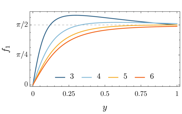
Figure 1. Profiles of $f_{1}$ in $d=3,4,5,6$.

$d$	$f_{1}^{\prime}(0)$	$f_{1}(1)$	$f_{1}^{\prime}(1)$
3	21.75741	$\pi/2$	$-0.30566$
4	10.9953	1.60634	$-0.10654$
5	7.82119	$\pi/2$	$0$
6	6.71508	1.53534	$0.059052$

Table 2. Shooting parameters of $f_{1}$ in $d=3,4,5,6$.

Numerical simulations of blowup require special methods that are able to resolve vanishing spatio-temporal scales as the solution develops a singularity. In our previous study of generic blowup for equation (3) we used a moving mesh method [1]. This method is computationally costly which is a serious drawback in the present context because the precise fine-tuning to the threshold requires many runs of the code. For this reason we propose here a different method which is based on specially designed similarity-like coordinates for which self-similar solutions are asymptotic stationary states. We believe that our method is interesting on its own and could be useful in numerical simulations of self-similar blowup for other evolution equations.

Note that standard similarity coordinates $(s,y)$ are not suitable for numerical evolution because the time of blowup is not known a priori which leads to the the gauge mode instability, as described above. To go around this difficulty we shall use a self-correcting coordinate system that adapts to the upcoming blow-up time as the solution evolves. This new coordinate system $(\tau,\rho)$ is defined as follows

$$r=e^{-\tau}\rho,\quad t=t(\tau),\quad\frac{dt}{d\tau}=e^{-\tau}h(\tau),$$ (23)

where the function $h(\tau)$, defining the relation between the numerical slow-time $\tau$ and $t$, will be chosen below (for $h=1$ the coordinates $(\tau,\rho)$ coincide with the similarity coordinates $(s,y)$). The new dependent variables $(V,P)$ are defined as follows

$$u(t,r)=V(\tau,\rho),\quad\partial_{t}u(t,r)=e^{\tau}P(\tau,\rho)\,.$$ (24)

In terms of these new variables the wave map equation takes the form

$$\partial_{\tau}V =hP-\rho\partial_{\rho}V,$$ (25a)

$$\partial_{\tau}P =h\left(\partial_{\rho\rho}V+\frac{d-1}{\rho}\partial_{\rho}V-\frac{d-1}{2\rho^{2}}\sin(2V)\right)-P-\rho\partial_{\rho}P.$$ (25b)

Differentiating (25a) with respect to $\rho$ and evaluating at $\rho=0$ we get

$$\partial_{\tau}(\partial_{\rho}V(\tau,0))+\partial_{\rho}V(\tau,0)=h(\tau)\partial_{\rho}P(\tau,0).$$ (26)

Choosing

$$h(\tau)=\left(\partial_{\rho}P(\tau,0)\right)^{-1}$$ (27)

and solving (26) we obtain

$$\partial_{\rho}V(\tau,0)=1+ce^{-\tau}.$$ (28)

Thus, regardless of whether the solution blows up or not, its gradient $\partial_{\rho}V(\tau,0)$ tends asymptotically to $1$. The gradient $\partial_{\rho}P(0,\tau)$ also remains bounded but its asymptotic value depends on an endstate of evolution. To see this, note that

$$\partial_{rt}u(t,0)=e^{2\tau}\partial_{\rho}P(\tau,0)\,,$$ (29)

which implies that in the case of dispersion we have $\partial_{\rho}P(0,\tau)\rightarrow 0$ (hence $h(\tau)\rightarrow\infty$), while in the case of blowup along the self-similar solution $f_{n}$ we have $\partial_{\rho}P(0,\tau)\rightarrow 1/f_{n}^{\prime}(0)$ (hence $h(\tau)\rightarrow f_{n}^{\prime}(0)$).

The boundedness of the gradient of any solution is a very desirable feature of our formulation since it allows us to solve the system (25), with $h$ given by (27), using standard finite difference methods on a uniform grid. More specifically, we use a fourth order centered finite difference scheme to approximate spatial derivatives in the interior of the numerical grid $0<\rho<\rho_{\textrm{max}}$. Near the origin $\rho=0$ we use symmetries of functions $V$ and $P$ to evaluate derivative stencils, while near the artificial boundary $\rho_{\textrm{max}}$ we use one-sided schemes. We evolve this semi-discrete system in time with fifth order adaptive Runge-Kutta method, known as DOPRI5 [9]. To suppress spurious high frequencies we add standard dissipation terms. As an outer boundary of the radial grid we typically take $\rho_{\text{max}}\approx 2f_{n}^{\prime}(0)$, where $f_{n}\left(\frac{r}{T-t}\right)$ is the expected self-similar endstate of evolution. This guarantees that the grid includes the past light cone of the singularity.

Remark.

Our numerical method can be viewed as a simplified moving mesh method combined with a Sundman transformation. In a moving mesh method each mesh point can move independently from other points (the motion of mesh points is governed by a prescribed mesh density function). In our case, the mesh points form a more rigid structure as reflected by a simple relation between $r$ and $\rho$. The relative scale of $r$ and $\rho$ is governed only by a single degree of freedom $h(\tau)$. The same parameter also dictates the relative scales of the time variables $t$ and $\tau$ just as a Sundman transformation would.

We illustrate our numerical results for initial data of the form

$$V(0,\rho)=\frac{A\rho}{\cosh{\rho}}=P(0,\rho)\,.$$ (30)

For large $A$ we find that $h(\tau)\rightarrow f_{0}^{\prime}(0)$ (which corresponds to generic blowup governed by the self-similar solution $f_{0}$), while for small $A$ we find that $h(\tau)\rightarrow\infty$ (which corresponds to dispersion to zero). Using bisection we fine tune the amplitude $A$ to the critical value $A_{*}$ with precision of 32 digits. For such marginally critical amplitudes we observe that for intermediate times $h(\tau)$ approaches $f_{1}^{\prime}(0)$. This is illustrated in Fig. 2 which shows the marginally sub- and supercritical evolutions in $d=6$ (the plots for $d=3,4,5$ look very similar).

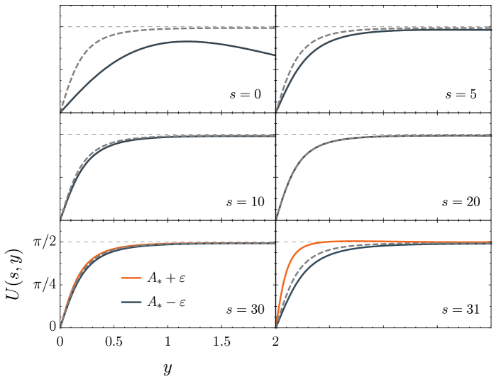
Figure 2. The evolution of a pair of initial data (30) in $d=6$ with marginally sub- (blue line) and supercritical (red line) amplitudes $A=A_{*}\pm\varepsilon$, where $\varepsilon$ is of the order $10^{-32}$. The solutions evolve together, approach the intermediate attractor $f_{1}$ (dashed line), and eventually depart from it in opposite directions.

To compare the results with the predictions of the linear perturbation analysis from section 3, we now translate the results into the similarity coordinates $(s,y)$. To this end we need to determine the blowup time $T$. This is done as follows. First, we integrate equation $\frac{dt}{d\tau}=e^{-\tau}h(\tau)$ to get $t(\tau)$. For intermediate times $t(\tau)$ develops a plateau which yields a rough estimate for $T$. Having that, we compute $e^{-s}=T-t$ and then

$$\partial_{y}U(s,0)\approx e^{\tau-s}\partial_{\rho}V(\tau,0).$$ (31)

From the linear perturbation analysis it follows that for intermediate times (when the solution is close to the threshold) the left hand side of (31) is well approximated by

$$\partial_{y}U(s,0)\approx f_{1}^{\prime}(0)+a_{1}e^{\lambda_{1}^{(1)}s}+a_{0}e^{s}+a_{-1}e^{\lambda_{-1}^{(1)}s},$$ (32)

where the coefficient $a_{1}\sim A-A_{*}$ is very small.

Since our estimate of the blowup time is not precise, this approximation involves the gauge mode instability with a nonzero coefficient $a_{0}(T)$. Fitting the formula (32) to the right hand side of (31), we get the coefficients $a_{1}$, $a_{0}$, and $a_{-1}$, which depend on the estimated value of $T$. Finally, performing bisection with respect to $T$ we determine the precise blowup time $T_{*}$ for which $a_{0}(T_{*})=0$.

The result of such a fit for the marginally critical evolution from Figure 2 is shown in Figure 3 (to plot both the sub- and supercritical solutions against the same variable $s=-\log(T-t)$, the blow-up time $T$ was chosen to be the average of $T_{*}$ for the sub- and supercritical solutions). The fit shows excellent agreement with the results of the linear perturbation analysis which makes us feel confident that our conjecture is true.

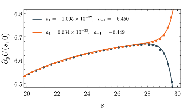
Figure 3. We plot the gradients at the origin for the marginally critical solutions shown in Figure 2. The gradients converge to $f_{1}^{\prime}(0)\approx 6.71$ with a rate given by the stable eigenvalue $\lambda_{-1}^{(1)}\approx-0.18$ and almost the same coefficients $a_{-1}$. At a later time, the gradients separate and stray away from $f_{1}^{\prime}(0)$, each growing with the rate given by the unstable eigenvalue $\lambda_{1}^{(1)}\approx 2.43$ and very small coefficients $a_{1}$ of opposite signs.

Acknowledgement. This research was supported in part by the Polish National Science Centre grant no. DEC-2012/06/A/ST2/00397. We gratefully acknowledge the support of the Alexander von Humboldt Foundation.

References

- [1] P. Bizoń, P. Biernat, Generic self-similar blowup for equivariant wave maps and Yang-Mills fields in higher dimensions, Commun. Math. Phys. 338, 1443 (2015)
- [2] P. Bizoń, T. Chmaj, and Z. Tabor, Dispersion and collapse of wave maps, Nonlinearity 13, 1411 (2000)
- [3] R. Donninger, On stable self-similar blowup for equivariant wave maps, Commun. Pure Appl. Math. 64, 1095 (2011)
- [4] P. Bizoń, Equivariant self-similar wave maps from Minkowski spacetime into 3-sphere, Commun. Math. Physics 215, 45 (2000)
- [5] J. Shatah, Weak solutions and development of singularities in the -model, Commun. Pure Appl. Math. 41, 459 (1988)
- [6] N. Turok, D. Spergel, Global texture and the microwave background, Phys. Rev. Lett. 64, 2736 (1990)
- [7] T. Cazenave, J. Shatah, A.S. Tahvildar-Zadeh, Harmonic maps of the hyperbolic space and the development of singularities in wave maps and Yang-Mills fields, Ann. Inst. Henri Poincaré 68, 315 (1998)
- [8] O. Costin, R. Donninger, I. Glogić, Mode stability of self-similar wave maps in higher dimensions, arXiv:1604.00303 [math.AP]
- [9] E. Hairer, S.P. Nørsett, G. Wanner, Solving ordinary differential equations I: Nonstiff problems, Springer-Verlag Berlin Heidelberg, 2008.