Multi-Path Feedback Recurrent Neural Networks for Scene Parsing

Abstract

In this paper, we consider the scene parsing problem and propose a novel Multi-Path Feedback recurrent neural network (MPF-RNN) for parsing scene images. MPF-RNN can enhance the capability of RNNs in modeling long-range context information at multiple levels and better distinguish pixels that are easy to confuse. Different from feedforward CNNs and RNNs with only single feedback, MPF-RNN propagates the contextual features learned at top layer through multiple weighted recurrent connections to learn bottom features. For better training MPF-RNN, we propose a new strategy that considers accumulative loss at multiple recurrent steps to improve performance of the MPF-RNN on parsing small objects. With these two novel components, MPF-RNN has achieved significant improvement over strong baselines (VGG16 and Res101) on five challenging scene parsing benchmarks, including traditional SiftFlow, Barcelona, CamVid, Stanford Background as well as the recently released large-scale ADE20K.

Introduction

Scene parsing has drawn increasing research interestdue to its wide applications in many attractive areas like autonomous vehicles, robot navigation and virtual reality. However, it remains a challenging problem since it requires solving segmentation, classification and detection simultaneously.

Recently, convolutional neural networks (CNNs) have been widely used for learning image representations and applied for scene parsing. However, CNNs can only capture high-level context information learned at top layers that have large receptive fields (RFs). The bottom layers are not exposed to valuable context information when they learn features. In addition, several recent works have demonstrated that even the top layers in a very deep model e.g. VGG16 (?) have limited RFs and receive limited context information (?) in fact. Therefore, CNNs usually encounter difficulties in distinguishing pixels that are easy to confuse locally and high-level context information is necessary. For example, in Figure 1, without the information of global context, the “field” pixels and “building” pixels are categorized incorrectly.

To address this challenge, we propose a novel multi-path feedback recurrent neural network (MPF-RNN). The overall architecture of our proposed MPF-RNN is illustrated in Figure 2. It has following two appealing characteristics. Firstly, MPF-RNN establishes recurrent connections to propagate downwards the outputs of the top layer to multiple bottom layers so as to fully exploit the context in the training process of different layers. Benefited from the enhanced context modeling capability, MPF-RNN gains a strong discriminative capability. Note that compared with previous RNN-based methods (?; ?) which use only one feedback connection from the output layer to the input layer and the layer-wise self-feedback connections, respectively, MPF-RNN is superior by using a better architecture, i.e. explicitly incorporating context information into the training process of multiple hidden layers, which learns concepts with different abstractness. Secondly, MPF-RNN effectively fuses the output features across different time steps for classification or a more concrete parsing purpose. We empirically demonstrate that such multi-step fusion greatly boosts the final performance of MPF-RNN.

To verify the effectiveness of MPF-RNN, we have conducted extensive experiments over five popular and challenging scene parsing datasets, including SiftFlow (?), Barcelona (?), CamVid (?), Stanford Background (?) and recently released large-scale ADE20K (?) and demonstrated that MPF-RNN is capable of greatly enhancing the discriminative power of per-pixel feature representations.

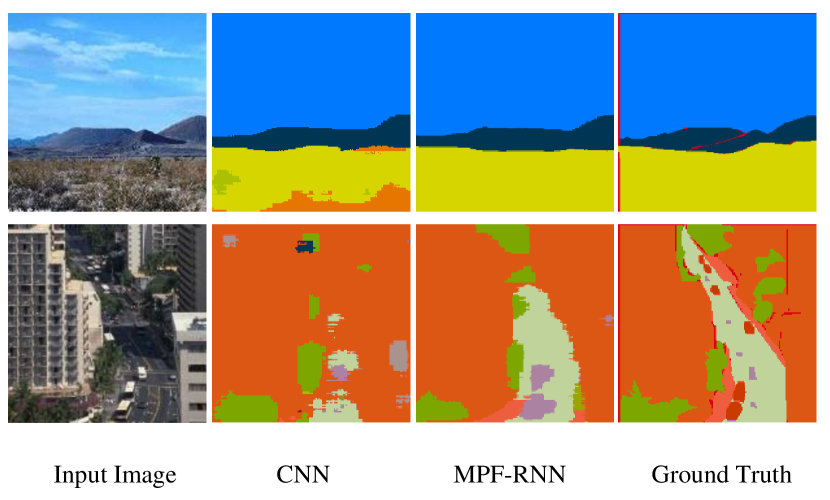
Figure 1: Illustration on importance of context information for distinguishing pixels. Without context, the field pixels in the first image are misclassified as desert. Similarly, the street pixels in the second image are misclassified as building. MPF-RNN can better model context information and thus produces more smooth and semantically meaningful parsing results. Best viewed in color.

Related Work

Image Context Modeling

One type of context modeling approaches for scene parsing is to use the probability graphical models (PGM) (e.g. CRF) to improve parsing results. In (?; ?; ?; ?; ?), CNN features are combined with a fully connected CRF to get more accurate parsing results. Compared to MPF-RNN, such methods usually suffer from intense calculation in inference due to their used time consuming mean field inference, which hinders their application in real-time scenario. Farabet et al. (?) encoded context information through surrounding contextual windows from multi-scale images. (?) proposed a recursive neural network to learn a mapping from visual features to the semantic space for pixel classification In (?), a parsing tree was used to propagate global context information. In (?), the global context feature is obtained by pooling the last layer’s output via global average pooling and then concatenated with local feature maps to learn a per-pixel classifier. Our method is different from them in both the context modeling scheme and the network architecture and achieves better performance.

Recurrent Neural Networks

RNN has been employed to model long-range context in images. For instance, (?) built one recurrent connection from the output to the input layer, and (?) introduced layer-wise self-recurrent connections. Compared with those methods, the proposed MPF-RNN models the context by allowing multiple forms of recurrent connections. In addition, MPF-RNN combines the output features at multiple time steps for pixel classification. (?) utilized a parallel multi-dimensional long short-term memory for fast volumetric segmentation. However, its performance was relatively inferior. (?; ?) were based on similar motivations that used RNNs to refine the learned features from a CNN by modeling the contextual dependencies along multiple spatial directions. In comparison, MPF-RNN incorporates the context information into the feature learning process of CNNs.

The MPF-RNN Model

Multi-Path Feedback

Throughout the paper, we use the following notations. For conciseness, we only consider one training sample. We denote a training sample as $(\mathbf{I},\mathbf{Y})$ where $\mathbf{I}$ is the raw image and $\mathbf{Y}$ is the ground truth parsing map of the image with $\mathbf{Y}_{i,j}\in\{1,\ldots,K\}$ as the ground truth category at the location $(i,j)$ in which $K$ is the number of categories. Since MPF-RNN is built upon CNNs by constructing recurrent connections from the top layer to multiple hidden layers, we therefore firstly consider a CNN composed of $L$ layers. Each layer outputs a feature map and we denote it as ${\mathbf{X}}^{\ell}$. Here ${\mathbf{X}}^{0}$ and ${\mathbf{X}}^{L}$ represent the input and final output of CNN. ${\mathbf{W}}^{\ell}$ denotes the parameter of filters or weights to be learned in the $l$-th layer. Using above notations, the outputs of an $L$-layered CNN at each layer can be written as

$$\mathbf{X}^{(\ell)}=f^{(\ell)}(\mathbf{W}^{(\ell)}\mathbf{X}^{(\ell-1)}),\ \ \ell=1,\ldots,L\,\ \ \text{and}\ \ \mathbf{X}^{(0)}\buildrel\Delta\over{=}\mathbf{I},$$ (1)

where ${\mathbf{W}}^{(\ell)}\mathbf{X}^{(\ell-1)}$ performs linear transformations on $\mathbf{X}^{(\ell-1)}$ and $f^{(\ell)}(\cdot)$ is a composite of multiple specific functions including the activation function, pooling and softmax. Here the bias term is absorbed into $\mathbf{W}^{(\ell)}$.

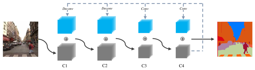
(a) MPF-RNN in recurrent format

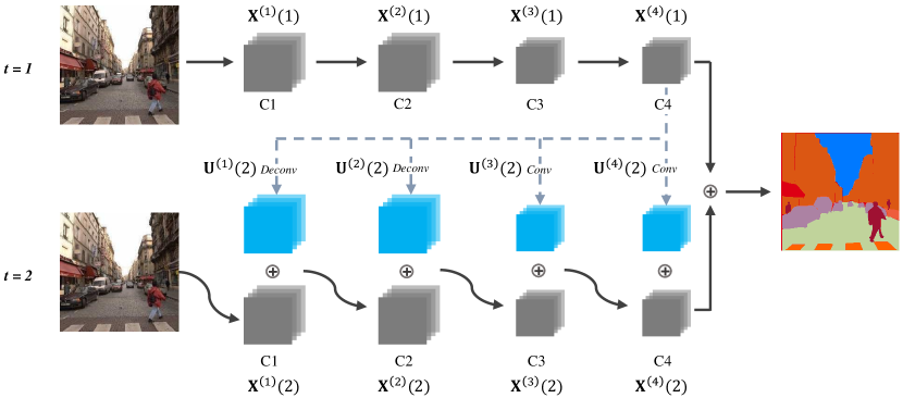
(b) Unfolded MPF-RNN

Figure 2: The framework of MPF-RNN. Top: an MPF-RNN built upon a shallow CNN of four convolution layers (i.e., C1 to C4) and shown in recurrent format. Multiple feedback connections are constructed from the top layer (C4) to hidden layers, the outputs of which are combined with the back-propagated features via an element-wise sum operation (denoted as $\oplus$). Convolution and deconvolution layers (i.e., Conv and Deconv) are used to model the feedback connections from C4 to hidden layers whose outputs have equal and larger spatial size than C4 respectively. Bottom: the corresponding unfolded MPF-RNN for two time steps. The parameters of convolution layers at different time steps are shared. To be discriminative to small objects, MPF-RNN combines output features across different time steps as the input for the pixel classifier which uses a deconvolution layer to produce the full-size labeling map. All notations in this figure are defined in Eqn. (2) and Eqn. (3).

MPF-RNN chooses $M$ layers out of $L$ layers and constructs recurrent connections from the top layer to each selected layer. Let $S=\{r_{m},m=1,\ldots,M\}$ denote the set of selected layers and let $r_{m}\in\{1,\ldots,L\}$ index the layers. By introducing the recurrent connections, each layer in $S$ takes both the output of its previous layer and the output of the top layer at the last time step as inputs. With $t$ denoting the index of time steps, Eqn. (1) can be rewritten as

$$\mathbf{X}^{(\ell)}(t)=\begin{cases}f^{(\ell)}(g^{(\ell)}(\mathbf{W}^{(\ell)}\mathbf{X}^{(\ell-1)}(t))\\ \qquad+g^{(\ell)}(\mathbf{U}^{(\ell)}(t)\mathbf{X}^{(L)}(t-1))),&\ell\in S,\\ f^{(\ell)}(\mathbf{W}^{(\ell)}\mathbf{X}^{(\ell-1)}(t)),&\text{otherwise},\end{cases}$$ (2)

where $\mathbf{X}^{(\ell)}(t)$ and $\mathbf{U}^{(\ell)}(t)$ denote the output of the $\ell$-th layer and the transformation matrix from the output of the $L$-th layer to the hidden layer $\ell\in S$ at time step $t$, respectively. Note that $\mathbf{W}^{(\ell)}$ is time-invariant, which means parameters in weight layers are shared across different time steps to reduce the model’s memory consumption. $\mathbf{U}^{(\ell)}(t)$ is time-variant so as to learn time step specific transformations for absorbing the context information from top layers. The output of top layers at different time steps conveys context information at different scales thus should have different transformations. The advantages of such a choice are verified in our experiments.

Following (?), function $g^{(\ell)}(\cdot)$ normalizes the input $\mathbf{x}$ as $g^{(\ell)}(\mathbf{x})=\gamma^{(\ell)}\mathbf{x}/||\mathbf{x}||_{2}$ where $\gamma^{(\ell)}$ is a learnable scaler and $||\mathbf{x}||_{2}$ denotes the $L_{2}$ norm of $\mathbf{x}$. As verified in (?), normalizing two feature maps output at different layers before performing combination is beneficial for convergence during training. One reason is that those two feature maps generally have different magnitude scales and they may slow down the convergence when their magnitudes are not balanced.

Now we proceed to explain the intuitions behind constructing multiple feedback connections. Since the RF of each layer in a deep neural network increases along with the depth, bottom and middle layers have relatively small RF. This limits the amount of context information that is perceptible when learning features in lower layers. Although higher layers might have larger RF and encode longer-range context, the context captured by higher layers cannot explicitly influence the states of the units in subsequent layers without top-down connections. Moreover, according to recent works (?; ?), the effective RF might be much smaller than its theoretical value. For example, in a VGG16 model, although the theoretical RF size for the top layer fc7 is equal to $224\times 224$, the effective RF size for the top layer fc7 is only about 1/4 of the theoretical RF. Due to the inadequate context information, layers in a deep model might not be able to learn context-aware features with strong discriminative power to distinguish local confusing pixels. Figure 1 shows examples of local confusion labeling by a CNN. To make layers in CNN incorporate context information, we therefore propose to propagate the output of the top layer to multiple hidden layers. Modulated with context, the deep model is context-aware when hierarchically learning concepts with different abstract levels. As a result, the model captures context dependencies to distinguish confusing local pixels. Actually, as the time step increases, the states of every unit in recurrent layers would have increasingly larger RF sizes and incorporate richer context.

We would also like to explain the reasons why we only build recurrent connections from the last layer: First, the last layer has the largest receptive field among all the layers whose output feature contains the richest contexts. Thus putting other layers in recurrent connections will introduce redundant context information and may hurt performance. Secondly, including more layers significantly increases computation cost. Only applying on the last layer gives a good trade-off between performance and efficiency.

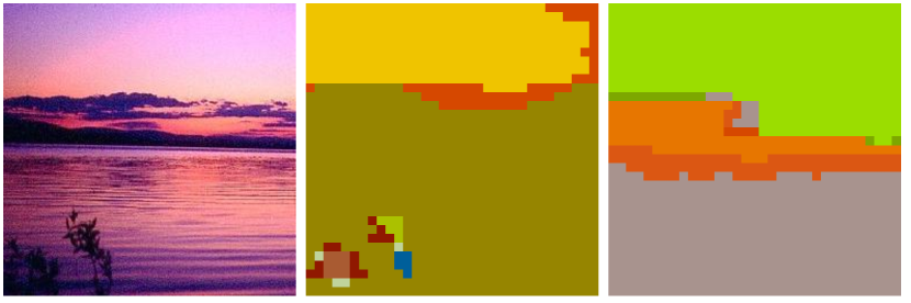
Figure 3: The features learned with a small number of time steps have stronger capability of depicting small objects compared to the features learned with a large number of time steps. Left: Input image. Middle: Output of fc7 at $t=1$. Right: Output of fc7 at $t=3$. The plant in the bottom-left coner of the left image is captured in the middle image but ignored in the right image.

Multi-Step Fusion Loss

As shown in Figure 2, MPF-RNN is trained through a back propagation through time (BPTT) method which is equivalent to unfolding the recurrent network to a deep feedforward network according to the time steps by sharing parameters of weight layers across different time steps. The conventional objective function is minimizing the weighted sum of cross-entropy losses between the output probability of the unfolded network and the binary per-pixel ground truth label.

There are two disadvantages with this objective function. First, features for small objects in an image might be inconspicuous in the higher-level feature map due to a stack of convolution and pooling operations, which hurts the parsing performance since scene images have many small objects. Secondly, since the depth of an unfolded feedforward model with many time steps is large, training bottom layers in early time steps may suffer from a vanishing gradient problem. To handle the above two disadvantages, we propose a new objective function with respect to the output feature maps from multiple time steps. Formally, the objective function we propose is given as

$$L=-\sum\limits_{(i,j)\in\mathbf{I}}{\mathbf{\omega}_{\mathbf{y}_{i,j}}\mathbf{h}_{\mathbf{y}_{i,j}}(\mathbf{w},\mathbf{O})},\mathbf{O}=\sum\limits_{t=1}^{T}{\lambda_{t}\mathbf{X}^{(L)}(t)}.$$ (3)

Here $T$ denotes the number of time steps, $\mathbf{O}$ denotes the combined feature of the top layer’s output at each time step, and $\mathbf{h}_{\mathbf{y}_{i,j}}(\mathbf{w},\mathbf{O})$ denotes the logarithmic prediction probability produced by a classifier which maps from input $\mathbf{O}$ to per-pixel category label $\mathbf{y}_{i,j}$. The specific formulation of $\mathbf{h}_{\mathbf{y}_{i,j}}(\mathbf{w},\mathbf{O})$ depends on the chosen classifier for predicting per-pixel label, such as MLP, SVM and logistic regression classifier, etc.

In our method, the classifier contains a deconvolution layer which resizes the discriminative representation $\mathbf{O}$ to be the same size as the input image for producing dense predictions, followed by a softmax loss layer to produce per-pixel categorical prediction probabilities. $\mathbf{w}$ denotes the parameters in the deconvolution layer. Note that $\mathbf{y}_{i,j}\in\{1,\ldots,L\}$ denotes the category of the pixel at location $(i,j)$. $\lambda_{t}$ balances the importance of feature maps at time step $t$ and $\mathbf{\omega}$ is the class weight vector. We further discuss them in the experiments.

The benefits of using Eqn. (3) are two-fold. On one hand, it improves MPF-RNN’s discriminability for small objects. Because the output features at later time steps have increasingly larger receptive field (RF) which receives wider-range context information, they may fail to distinguish small objects. In contrast, output features at earlier time steps have smaller RF and are more discriminative in capturing small objects. Therefore the combination of features in the last time step with those of ealier time steps helps the model identify small objects. On the other hand, for deep models with hundreds or thousands layers and large time steps, it may avoid the gradient vanishing problem in bottom layers at early time steps by giving shorter paths from them to the loss layer. Note that the multi-step fusion used in our method is different from the feature fusion method used in FCN (?). While FCN combines feature maps from hidden layers in a CNN, we combine the outputs at different time steps in an RNN model, which retains stronger context modeling capabilities.

Discussions

To better understand MPF-RNN, we compare it with several existing RNN models. Conventional RNN is trained with a sequence of inputs $\{x^{(t)}\}_{t=1:T}$ by computing the following sequences: $h^{(t)}=s(Ux^{(t)}+Wh^{(t-1)})$ and $y^{(t)}=z(Vh^{(t)})$,
where $h^{(t)}\mbox{and}\ y^{(t)}$ are the hidden layer and output layer at time step $t$, respectively, while $U\mbox{and}\ W$ are weights matrices between the input and hidden layers, and among the hidden units themselves, respectively. $V$ is the output matrix between hidden and output layers. $s(\cdot)\mbox{ and}\ z(\cdot)$ are activation functions. Compared with the conventional RNNs, MPF-RNN has multiple recurrent connections from the output layer to hidden layers (as indicated by Eqn. (2)) and moreover, MPF-RNN combines the outputs of multiple time steps as the final output (see Eqn. (3)).

Compared with those two recently proposed RNN-based models (?; ?), which have one recurrent connection from the output layer to the input layer and layer-wise self-recurrent connections, respectively, our model can be deemed as a generalization by allowing more general recurrent connections. Specifically, when $1\in S$ (recall $S$ is the index set of selected layers with which the output layer has feedback connections), there will be a recurrent connection from the output layer to the input layer in our model, as in (?); when $L\in S$, there will be self-recurrent connections, as in (?). By utilizing context information in different layers, our model has a stronger capability to learn discriminative features for each pixel. We also highlight the main difference of network architecture between MPF-RNN and RCN (?). RCN is still essentially a feed-forward network which utilizes features in higher layers to aggregate features in bottom layer for facial keypoint localization problem, while MPF-RNN is a novel RNN architecture for better modeling the long-range context information in scene parsing problem.

The way to build multiple recurrent connections from the top layer to subsequent layers is a reminiscent of fully recurrent nets (FRN) (?) which is an MLP with each non-input unit receiving connections from all the other units. Different from FRN, we employ convolution/deconvolution layers to model the recurrent connections in MPF-RNN so as to preserve the spatial dependencies of 2D images. Besides, we do not build recurrent connections from the output layer to every subsequent layer, since the neighboring layers contain redundant information and the “fully recurrent” way is prone to over-fitting in scene parsing tasks. In addition, we perform multi-step fusion to improve the final performance, while FRN only uses the output of the final layer. To the best of our knowledge, we are among the first to apply multiple convolutional recurrent connections for solving scene parsing problems.

Experiments

Experiment Settings and Implementation Details

Evaluation Metrics

Adopted by most previous works as evaluation metrics, the per-pixel accuracy (PA) and the average per-class accuracy (CA) are used. PA is defined as the percentage of all correctly classified pixels while CA is the average of all category-wise accuracies.

Baseline Models

Following (?), we use a variant of the ImageNet pre-trained VGG16 network as the baseline model and fine-tune it on four scene parsing datasets, including SiftFlow, Barcelona, CamVid and Stanford Background. Here, fully connected (FC) layers (fc6 and fc7) are replaced by convolution layers. To accelerate the dense labeling prediction, the kernel size of fc6 is reduced to $3\times 3$ and the number of channels at FC layers is reduced to 1,024. This model is referred to as “VGG16-baseline” in the following experiments. Note that the VGG16-baseline model is equivalent to the MPF-RNN model with time step equal to 1. For simplicity, in the following text, we denote conv5 as conv5_1, conv4 as conv4_1 and conv3 as conv3_1.

Multi-Path Feedback

A practical problem with using MPF-RNN is how to choose the layer set $S$, to which the recurrent connections from the top layer are constructed. There are two thumb rules. First, the layers at very bottom should not be chosen since they generally learn basic and simple patterns like edges, circles and dots, in which global context is not helpful. Secondly, it should be avoided to choose too many neighboring layers so that abundant information may be reduced in the features learned from neighboring layers. Following the above two rules, we conduct experiments with various $S$ on the validation set of SiftFlow and choose the one with best validation performance. The comparative results are shown in Table 1, from which we can see that choosing $S=\{\text{conv}4,\text{conv}5,\text{fc}6,\text{fc}7\}$ gives the best performance.

Multi-Step Fusion

There is a trade-off between the computation efficiency and model complexity when choosing the number of time steps for unfolding MPF-RNN. A deeper network can learn more complex features and give better performance. On the other hand, a large model is time consuming to train and test, which turns out to be problematic when applied to real-time scenarios, e.g. automatic driving. Table 2 compares the performance of MPF-RNN with different time steps on SiftFlow, from which we observe that among other time steps, $T=3$ achieves the best performance with fast speed. Therefore, we choose $T=3$ as the default time step for all datasets. Besides, we set $\lambda_{1}=\lambda_{2}=0.3$ and $\lambda_{3}=1$ throughout our experiments. As an alternative, we can also see $\lambda_{t}$ as learnable parameters and train them jointly with the whole model end-to-end. However, we do not explore this method in the paper.

Hyperparameters

The hyperparameters introduced by MPF-RNN, including $S,T$ and $\lambda$ are fine-tuned on the validation set of SiftFlow as introduced above and then fixed for other datasets where MPF-RNN uses VGG16 network. Our experiments verified that such values of hyperparameters are optimum in all datasets.

Loss Re-Weighting

Since in scene parsing tasks, the class distribution is extremely unbalanced, it is common to re-weight different classes during training to attend rare classes (?; ?). In our model, we adopt the reweighting strategy by (?) because of its simplicity and effectiveness. Briefly, the weight for class $\mathbf{y}_{i,j}$ is defined as $\omega_{\mathbf{y}_{i,j}}=2^{\left\lceil{\log 10(\eta/f_{\mathbf{y}_{i,j}})}\right\rceil}$ where $f_{\mathbf{y}_{i,j}}$ is the frequency of class $\mathbf{y}_{i,j}$ and $\eta$ is a dataset-dependent scalar, which is defined according to 85%/15% frequent/rare classes rule.

Fine-Tuning Strategy

Our model is fine-tuned over target datasets using the stochastic gradient descent algorithm with momentum. For models using VGG16 network, settings of hyper-parameters including learning rate, weight decay and momentum follow (?). The reported results are based on the model trained in 40 epochs. Data augmentation is used to reduce the risk of over-fitting and improve the generalization performance of deep neural network models. To make a fair comparison with other state-of-the-art methods, we only adopt the common random horizontal flipping and cropping during training.

Computational Efficiency

On a NVIDIA Titan X GPU, the training of MPF-RNN (the model in Table 3) on SiftFlow dataset finishes in about 6 hours and the testing time for an image with the resolution of 256$\times$256 is 0.06s.

Table 1: Comparative study of effects of different recurrent connections on final performance of MPF-RNN over SiftFlow dataset. The time step of MPF-RNN is fixed as 2 in all experiments in this table. The best results are shown in bold.

Recurrent connections	PA(%)	CA(%)
VGG16-baseline	84.7	51.5
{fc7}	85.4	55.1
{fc6, fc7}	85.9	55.5
{conv5, fc6, fc7}	86.2	55.8
{conv4, conv5, fc6, fc7}	86.4	56.3
{conv3, conv4, conv5, fc6, fc7}	85.9	55.7

Results

We test MPF-RNN on five challenging scene parsing benchmarks, including SiftFlow (?), Barcelona (?), CamVid (?), Stanford Background (?) and ADE20K. We report the quantitative results here and more qualitative results of MPF-RNN are given in the Supplementary Material.

SiftFlow

The SiftFlow dataset (?) consists of 2,400/200 color images with 33 semantic labels for training and testing.

Table 2: Comparative study of effects of different recurrent time steps and multi-step fusion (MSF) on final performance of MPF-RNN over SiftFlow dataset. $S=\{\text{conv}4,\text{conv}5,\text{fc}6,\text{fc}7\}$ herein.

	w/ MSF		w/o MSF
Time steps	PA(%)	CA(%)	PA(%)	CA(%)
VGG16-baseline	84.7	51.5	N.A.	N.A.
T = 2	86.4	56.3	86.0	55.5
T = 3	86.9	56.5	85.2	55.1
T = 4	86.8	55.9	84.7	54.8

Model Analysis We analyze the MPF-RNN by investigating the effects of its two important components separately, i.e. multi-path feedback and multi-step fusion. Table 1 lists the performance of MPF-RNN, as well as the baseline models when different recurrent connections are used. The number of time steps is set as 2 for all MPF-RNN models and combination weights are $\lambda_{1}=0.3$ and $\lambda_{2}=1$. Compared with the baseline model which has achieved 84.7%/51.5% PA/CA on this dataset, adding recurrent connections to multiple subsequent layers significantly improves the performance in terms of PA and CA. Only adding one recurrent connection to the layer fc7 can increase the performance to 85.4%/55.1%, which proves the benefit of global context modulating to the performance. Continuing adding recurrent connections to conv5 and conv4 consistently improves the performance. The reason for the continuous improvement is the sufficient utilization of the context information in learning context-aware features in different hidden layers. Based on above experimental results, it is verified that multi-path feedback is beneficial for boosting the performance of scene parsing systems. We also note that the performance tends to slow down its increasing (although still much higher than the baseline model) when adding too many recurrent connections ($S=\{\text{conv4, conv5, fc6, fc7}\}$). Such a phenomenon implies the overfitting due to the increased number of parameters.

Table 3: Comparison with the state-of-the-art methods on SiftFlow.

Methods	PA(%)	CA(%)
Tighe et al. (?)	79.2	39.2
Sharma et al. (?)	79.6	33.6
Singh et al. (?)	79.2	33.8
Yang et al. (?)	79.8	48.7
Liang et al. (?)	84.3	41.0
Long et al. (?)	85.2	51.7
Liu et al. (?)	86.8	52.0
Shuai et al. (?)	85.3	55.7
MPF-RNN(ours)	86.9	56.5

Table 2 shows the effects of different time steps and multi-step fusion on the performance. We conduct experiments when $T=1,2,3,4$ by setting $S=\{\text{conv4, conv5, fc6, fc7}\}$. Concluded from Table 2, the PA/CA consistently improves from $T=1$(VGG16-baseline) to $T=3$. Such improvement is attributed to the more complex discriminative features learned using larger time steps, which is proportional to the depth of the feedforward deep model after MPF-RNN is unfolded. The improvement is also consistent with observations in (?; ?; ?) that deeper and larger models have stronger feature representation capabilities compared with shallow ones. When $T=4$, the performance is worse than that when $T=3$ due to the overfitting problem.

We also conduct experiments when only the top layer’s feature in the last time step is used as the input to the classifier. Specifically, we set $\lambda_{t}=0,t=2,\cdots,T$ and $\lambda_{T}=1$ and keep the other conditions unchanged. It is observed from Table 2 that under any time steps, the PA/CA are worse than those when multi-step fusion is applied. There are two reasons for the inferior performance. Updating bottom layers parameters is insufficient since it takes many hidden layers to propagate the error message from the output layer to bottom layers. In addition, as illustrated in Figure 3, the output layer at the last time step might ignore small objects, which could otherwise be complemented by using multi-step fusion. Above experiment demonstrates the effectiveness of multi-step fusion. Note that although the conclusions made in model analysis are based on the results on SiftFlow, we have verified through experiments that they also hold on other three datasets where MPF-RNN uses VGG16 network.

Comparison with State-of-the-Art The comparison results of MPF-RNN with other state-of-the-art methods are shown in Table 3, from which we can see that MPF-RNN achieves the best performance against all the compared methods. Specifically, our method significantly outperforms Pinheiro et al. (?) and Liang et al. (?) by increasing the PA/CA by 9.2%/26.7% and 2.6%/15.5%, respectively. Note that  (?) and  (?) are all RNN-based methods. The remarkable improvement of MPF-RNN over them is attributed to MPF-RNN’s powerful context modeling strategy by constructing multiple recurrent connections in various forms. Compared with (?), MPF-RNN achieves much better CA due to its superior capability of distinguishing small objects.

ADE20K

To further verify scalability of the MPF-RNN to large-scale dataset and deeper networks, we conduct experiments using ResNet101 (?) on recently released ADE20K dataset (?) which also serves as the dataset of scene parsing challenge in ILSVRC16. Containing 20K/2K/3K fully annotated scene-centric train/val/test images with 150 classes, ADE20K has more diverse scenes and richer annotations compared to other scene parsing dataset, which make it a challenging benchmark. Following (?), all convolution layers in original ResNet101 (?) after conv3_4 are replaced with dilated convolution layers to compute dense scores at stride of 8 pixels, followed by a deconvolution layer to reach original image resolution. This model is used as a strong baseline and referred to as ResNet101-Baseline. Since the test set is not available till submission of the paper, we use the val set to test the performance of MPF-RNN. In order to fine-tune hyperparameters, we randomly extract 2K images from train set as our validation data and retrain our model using whole train set after fixing hyperparameters. Through validation, we set $S=\{\text{conv}4\textunderscore 1,\text{conv}4\textunderscore 9,\text{conv}4\textunderscore 17,\text{conv}5\textunderscore 1,\text{conv}5\textunderscore 3\}$ and the value of $T$ and $\lambda$ are the same as those in the last section. MPF-RNN and ResNet101-Baseline are trained for 20 epochs by fine-tuning ResNet101 on ADE20K with the same solver configurations of (?). Data augmentation only include random horizontal flipping and cropping. We do not use loss re-weighting in this dataset.

Table 4: Comparison results of MPF-RNN on ADE20K val set. The results of FCN, SegNet and DilatedNet are referred from the reported number in (?)

Methods	PA(%)	mIOU(%)
FCN (?)	71.32	29.39
SegNet (?)	71.0	21.64
DilatedNet (?)	73.55	32.31
Res101-Baseline	73.71	32.65
MPF-RNN (ours)	76.49	34.63

In Table 4, we compare the performance of MPF-RNN and baseline models. Following the evaluation metric in ILSVRC16 scene parsing challenge, we compare the PA and mean IOU (the mean value of intersection-over-union between the predicted and ground-truth pixels across all classes) between different models. It is observed from Table 4 that Res101-Baseline has achieved better performance compared to other models based on VGG16 due to its superior deep architecture. By using MPF-RNN, MPF-RNN significantly surpasses this strong baseline model by 2.78%/1.98 in terms of PA/mIOU, again demonstrating the capability of MPF-RNN to improve the scene parsing performance of deep networks.

Results on Other Datasets

We further evaluate MPF-RNN on Barcelona, Stanford Background and Camvid datasets. MPF-RNN achieves the best performance on these three datasets: (i) Stanford Background: $86.6\%$ (PA) and $79\%$ (CA), outperforming state-of-the-art with $3\%$ (PA) and $5\%$ (CA) absolutely; (ii) Barcelona: $78.5\%$ (PA) and $29.3\%$ (CA) higher than state-of-the-art with around $4\%$ (PA) and $5\%$ (CA) absolutely; (iii) Camvid: $92.8\%$ (PA) and $82.3\%$ (CA), outperforming state-of-the-art with $1\%$ (PA) and $4\%$ (CA) absolutely. Due to space limits, more numbers and details of experimental results on these three datasets are deferred to the supplementary material.

Conclusion

We proposed a novel Multi-Path Feedback recurrent neural network (MPF-RNN) for better solving scene parsing problems. In MPF-RNN, multiple recurrent connections are constructed from the output layer to hidden layers. To learn features discriminative for small objects, output features at each time step are combined for per-pixel prediction in MPF-RNN. Experimental results over five challenging scene-parsing datasets, including SiftFlow, ADE20K, Barcelona, Stanford Background, and CamVid clearly demonstrated the advantages of MPF-RNN for scene parsing.

Acknowledgement

Xiaojie Jin is immensely grateful to Bing Shuai at NTU and Wei Liu at UNC - Chapel Hill for valuable discussions. The work of Jiashi Feng was partially supported by National University of Singapore startup grant R-263-000-C08-133 and Ministry of Education of Singapore AcRF Tier One grant R-263-000-C21-112.

See pages 1-3 of supp

References

- [Badrinarayanan, Kendall, and Cipolla 2015] Badrinarayanan, V.; Kendall, A.; and Cipolla, R. 2015. Segnet: A deep convolutional encoder-decoder architecture for image segmentation. CoRR abs/1511.00561.
- [Brostow et al. 2008] Brostow, G. J.; Shotton, J.; Fauqueur, J.; and Cipolla, R. 2008. Segmentation and recognition using structure from motion point clouds. In ECCV.
- [Chen et al. 2015] Chen, L.-C.; Papandreou, G.; Kokkinos, I.; Murphy, K.; and Yuille, A. L. 2015. Semantic image segmentation with deep convolutional nets and fully connected crfs. In ICLR.
- [Chen et al. 2016] Chen, L.; Papandreou, G.; Kokkinos, I.; Murphy, K.; and Yuille, A. L. 2016. Deeplab: Semantic image segmentation with deep convolutional nets, atrous convolution, and fully connected crfs. CoRR abs/1606.00915.
- [Farabet et al. 2013] Farabet, C.; Couprie, C.; Najman, L.; and LeCun, Y. 2013. Learning hierarchical features for scene labeling. TPAMI 35(8):1915–1929.
- [Gould, Fulton, and Koller 2009] Gould, S.; Fulton, R.; and Koller, D. 2009. Decomposing a scene into geometric and semantically consistent regions. In ICCV.
- [He et al. 2015] He, K.; Zhang, X.; Ren, S.; and Sun, J. 2015. Deep residual learning for image recognition. arXiv preprint arXiv:1512.03385.
- [Honari et al. 2015] Honari, S.; Yosinski, J.; Vincent, P.; and Pal, C. 2015. Recombinator networks: Learning coarse-to-fine feature aggregation. arXiv preprint arXiv:1511.07356.
- [Liang, Hu, and Zhang 2015] Liang, M.; Hu, X.; and Zhang, B. 2015. Convolutional neural networks with intra-layer recurrent connections for scene labeling. In NIPS.
- [Liu, Rabinovich, and Berg 2015] Liu, W.; Rabinovich, A.; and Berg, A. C. 2015. Parsenet: Looking wider to see better. arXiv preprint arXiv:1506.04579.
- [Liu, Yuen, and Torralba 2009] Liu, C.; Yuen, J.; and Torralba, A. 2009. Nonparametric scene parsing: Label transfer via dense scene alignment. In CVPR.
- [Long, Shelhamer, and Darrell 2015] Long, J.; Shelhamer, E.; and Darrell, T. 2015. Fully convolutional networks for semantic segmentation. In CVPR.
- [Pinheiro and Collobert 2013] Pinheiro, P. H., and Collobert, R. 2013. Recurrent convolutional neural networks for scene parsing. arXiv preprint arXiv:1306.2795.
- [Roy and Todorovic 2014] Roy, A., and Todorovic, S. 2014. Scene labeling using beam search under mutex constraints. In CVPR.
- [Schwing and Urtasun 2015] Schwing, A. G., and Urtasun, R. 2015. Fully connected deep structured networks. arXiv preprint arXiv:1503.02351.
- [Sharma, Tuzel, and Liu 2014] Sharma, A.; Tuzel, O.; and Liu, M.-Y. 2014. Recursive context propagation network for semantic scene labeling. In NIPS.
- [Shuai et al. 2015] Shuai, B.; Zuo, Z.; Wang, G.; and Wang, B. 2015. Dag-recurrent neural networks for scene labeling. arXiv preprint arXiv:1509.00552.
- [Simonyan and Zisserman 2014] Simonyan, K., and Zisserman, A. 2014. Very deep convolutional networks for large-scale image recognition. arXiv preprint arXiv:1409.1556.
- [Singh and Kosecka 2013] Singh, G., and Kosecka, J. 2013. Nonparametric scene parsing with adaptive feature relevance and semantic context. In CVPR.
- [Socher et al. 2011] Socher, R.; Lin, C. C.; Manning, C.; and Ng, A. Y. 2011. Parsing natural scenes and natural language with recursive neural networks. In ICML.
- [Stollenga et al. 2015] Stollenga, M. F.; Byeon, W.; Liwicki, M.; and Schmidhuber, J. 2015. Parallel multi-dimensional lstm, with application to fast biomedical volumetric image segmentation. In NIPS, 2998–3006.
- [Szegedy et al. 2014] Szegedy, C.; Liu, W.; Jia, Y.; Sermanet, P.; Reed, S.; Anguelov, D.; Erhan, D.; Vanhoucke, V.; and Rabinovich, A. 2014. Going deeper with convolutions. arXiv preprint arXiv:1409.4842.
- [Tighe and Lazebnik 2010] Tighe, J., and Lazebnik, S. 2010. Superparsing: scalable nonparametric image parsing with superpixels. In ECCV.
- [Visin et al. 2015] Visin, F.; Kastner, K.; Courville, A. C.; Bengio, Y.; Matteucci, M.; and Cho, K. 2015. Reseg: A recurrent neural network for object segmentation. CoRR abs/1511.07053.
- [Williams and Zipser 1989] Williams, R. J., and Zipser, D. 1989. A learning algorithm for continually running fully recurrent neural networks. Neural computation 1(2):270–280.
- [Yang et al. 2014] Yang, J.; Price, B.; Cohen, S.; and Yang, M.-H. 2014. Context driven scene parsing with attention to rare classes. In CVPR.
- [Yu and Koltun 2015] Yu, F., and Koltun, V. 2015. Multi-scale context aggregation by dilated convolutions. CoRR abs/1511.07122.
- [Zhang and Chen 2012] Zhang, Y., and Chen, T. 2012. Efficient inference for fully-connected crfs with stationarity. In CVPR.
- [Zheng et al. 2015] Zheng, S.; Jayasumana, S.; Romera-Paredes, B.; Vineet, V.; Su, Z.; Du, D.; Huang, C.; and Torr, P. H. 2015. Conditional random fields as recurrent neural networks. In ICCV.
- [Zhou et al. 2014] Zhou, B.; Khosla, A.; Lapedriza, A.; Oliva, A.; and Torralba, A. 2014. Object detectors emerge in deep scene cnns. arXiv preprint arXiv:1412.6856.
- [Zhou et al. 2016] Zhou, B.; Zhao, H.; Puig, X.; Fidler, S.; Barriuso, A.; and Torralba, A. 2016. Semantic understanding of scenes through the ade20k dataset. arXiv preprint arXiv:1608.05442.