Time-dependent solutions for a stochastic model of gene expression with molecule production in the form of a compound Poisson process

Abstract

We study a stochastic model of gene expression, in which protein production has a form of random bursts whose size distribution is arbitrary, whereas protein decay is a first-order reaction. We find exact analytical expressions for the time evolution of the cumulant-generating function for the most general case when both the burst size probability distribution and the model parameters depend on time in an arbitrary (e.g. oscillatory) manner, and for arbitrary initial conditions. We show that in the case of periodic external activation and constant protein degradation rate, the response of the gene is analogous to the RC low-pass filter, where slow oscillations of the external driving have a greater effect on gene expression than the fast ones. We also demonstrate that the $n$-th cumulant of the protein number distribution depends on the $n$-th moment of the burst size distribution. We use these results to show that different measures of noise (coefficient of variation, Fano factor, fractional change of variance) may vary in time in a different manner. Therefore, any biological hypothesis of evolutionary optimization based on the nonmonotonicity of a chosen measure of noise must justify why it assumes that biological evolution quantifies noise in that particular way. Finally, we show that not only for exponentially distributed burst sizes but also for a wider class of burst size distributions (e.g. Dirac delta and gamma) the control of gene expression level by burst frequency modulation gives rise to proportional scaling of variance of the protein number distribution to its mean, whereas the control by amplitude modulation implies proportionality of protein number variance to the mean squared.

I Introduction

It has been confirmed experimentally that in living cells both mRNA Golding et al. (2005) and protein Ozbudak et al. (2002); Cai et al. (2006); Yu et al. (2006); Taniguchi et al. (2010); Choi et al. (2008) production may take form of stochastic bursts of a random size. The presence of bursts may be a result of processes involving short-lived molecules (e.g. the mRNA in case of protein production), concentration of which may be treated as a fast degree of freedom Friedman et al. (2006); Shahrezaei and Swain (2008). The number of protein molecules that can be produced from a single mRNA molecule before the latter is degraded is a random variable, and its distribution may, in the several experimentally known cases, be well approximated by geometric or exponential distribution Cai et al. (2006); Yu et al. (2006); Taniguchi et al. (2010). For that reason, in most of the existing models of bursty gene expression, the exponential (or geometric in a discrete case) bursts of protein Paulsson and Ehrenberg (2000); Friedman et al. (2006); Shahrezaei and Swain (2008); Aquino et al. (2012); Lin and Galla (2016) or mRNA Aquino et al. (2012) production are considered.

However, in the case of eukaryotic cells, certain models predict nonexponential distributions of burst sizes Schwabe et al. (2012); Elgart et al. (2011); Kuwahara et al. (2015). In particular, in the case of transcriptional bursts the molecular ratchet model predicts peaked distributions, that resemble gamma distribution Schwabe et al. (2012). Therefore, it seems desirable to study the analytically tractable models of bursty gene expression dynamics with a general, nonexponential form of burst size distributions.

Also, for the majority of stochastic models of gene expression proposed to date, even if the time-dependent solutions are considered Iyer-Biswas et al. (2009); Tabaka and Hołyst (2010); Ramos et al. (2011); Feng et al. (2012); Pendar et al. (2013); Kumar et al. (2014), it is usually assumed that model parameters are time-independent. However, taking into account the time variation of the model parameters, in particular the periodic time dependence of the rate of protein production Mugler et al. (2010) gives us an opportunity to model in a simple manner the response of a genetic circuit to oscillatory regulation and to indicate some qualitative properties of solutions for other oscillating parameters.

In this paper, we investigate a simple gene expression model, which is a natural generalization of the analytical framework proposed in Ref. Friedman et al. (2006), and which may serve as a model of both transcription and translation Aquino et al. (2012). Namely, in contrast to Ref. Friedman et al. (2006) we consider the case of an arbitrary (not necessarily exponential) burst size probability distribution and time-dependent model parameters. However, gene autoregulation is neglected. To the best of our knowledge, the time-dependent solutions of the model of Ref. Friedman et al. (2006) have not been known to date even in the absence of gene autoregulation or for the simplest case of time-independent model parameters.

We find the explicit time dependence of the cumulant-generating function for the probability distribution of molecule (protein) concentration. This general result is then applied to describe the oscillatory response of a gene to periodic modulation of the rate of protein production. In particular, we consider a gene driven by a single-frequency, sinusoidal regulation. In such a case, the time dependence of the mean molecule concentration consists of both the transient, exponentially decaying part and of the periodic part, whose amplitude depends on the driving frequency. We also point out that the division of the system’s response into periodic and transient part remains true in a more general case, when the model parameters are periodic functions of time.

We also show a simple relationship that links the $n$-th cumulant of the protein number distribution and the $n$-th moment of the burst size distribution. In particular, this relationship is proportional in the steady state. We use these results to discuss the question of possible evolutionary optimization of cellular processes with respect to noise intensity. Since it has been shown experimentally that distributions of protein numbers have universal scaling properties (variance proportional to mean or variance proportional to mean squared) Salman et al. (2012); Bar-Even et al. (2006), we use our results to gain an insight into possible origins of such scalings in the properties of the burst size distributions.

Stochastic models with bursty dynamics similar to the model considered here are known both in mathematics (so-called Takacs processes Cox and Isham (1986); Takacs et al. (1961)) and in physics (under the name of compound Poisson processes), where such models are used not only to describe stochastic dynamics of transcription or translation, but also to model such diverse phenomena as diffusion with jumps Luczka et al. (1995); Czernik et al. (1997); Łuczka et al. (1997), time dependence of soil moisture Porporato and D’Odorico (2004); Daly and Porporato (2006, 2010); Suweis et al. (2011); Mau et al. (2014), dynamics of snow avalanches Perona et al. (2012), statistics of the solar flares Wheatland (2008, 2009) and oil prices on the stock market Askari and Krichene (2008). And therefore, our results may be relevant to other fields beyond stochastic modeling of gene expression.

II Results

Let us consider a source (gene) that creates objects (protein or mRNA molecules) of a single type, denoted by X, which are subsequently degraded or diluted due to the system size expansion, e.g. cell growth and division,

DNA $$\xrightarrow{I(t)} \text{X},~{}~{}~{}~{}~{}\text{X}\xrightarrow{\gamma(t)}\emptyset.$$ (1)

We focus on the simplest situation, when the molecules interact neither with each other, nor with the source. In consequence, the probability of degradation of a single molecule does not depend on the total number of molecules in the system. This assumption leads to a linear decay process (first-order reaction), which is the simplest, but arguably the most natural choice here. Still, we assume that both the source intensity ${I(t)}$ and the decay parameter $\gamma(t)$ may vary with time in an arbitrary manner. Therefore, although we assume that the characteristics of the source are independent on the number of molecules present in the system (feedback effects are neglected), we allow the source (gene) to be externally regulated. If the number of molecules is sufficiently large, the continuous approximation is justified and the molecule concentration may be used instead of the exact copy number of molecules.

In order to obtain the stochastic description of the system, we assume that the molecule production takes the form of bursts of random size. Namely, the number of newly created molecules (or the magnitude of a concentration jump in the present continuous model), $u$, is a stochastic variable drawn from the probability distribution $\nu(u,t)$, which may be explicitly time-dependent. It is assumed here, that burst duration is short enough that even large bursts can be treated as instantaneous. The time of appearance of each burst is also a random variable.

The occurrence of stochastic bursts in a given system may be due to the presence of some processes that are much faster than production or degradation of molecules in question; such processes are not explicitly taken into account within the model. For example, translational bursts of proteins are attributed to the existence of short-lived mRNA molecules Shahrezaei and Swain (2008); Lin and Galla (2016). However, it is not our aim here to relate the functional form of the burst size probability distribution to dynamics of fast degrees of freedom. Rather, we treat bursty dynamics as a well-justified approximation leading to reasonable effective description of the system at hand.

The deterministic model describing the kinetics of reactions (1) is given by a simple rate equation (60), see Appendix A. Its stochastic counterpart is the following Langevin-like equation

$$\dot{x} = I(t)-\gamma(t)x,$$ (2)

where $x\geq 0$ is the molecule concentration and dot denotes the time derivative. $I(t)$ appearing in (2) is now a compound Poisson process, i.e.

$$I(t) = \sum_{k=1}^{N(t)}u_{k}\delta(t-t_{k}),$$ (3)

where $u_{k}$ is the size of the molecule burst (concentration jump) that takes place at $t=t_{k}$ and $N(t)$ is the number of concentration jumps in the interval $[0,t)$.

Stochastic differential equations similar to (2) have been used to model diffusion in asymmetric periodic potentials Luczka et al. (1995); Czernik et al. (1997); Łuczka et al. (1997), soil moisture dynamics and other phenomena in geophysics Perona et al. (2012); Porporato and D’Odorico (2004); Daly and Porporato (2006, 2010); Suweis et al. (2011); Mau et al. (2014), astrophysics Wheatland (2008, 2009) and economics Askari and Krichene (2008).

Instead of Eq. (2) it is more convenient to study the corresponding master equation, proposed in Ref. Friedman et al. (2006)

$$\frac{\partial p(x,t)}{\partial t} = \gamma(t)\frac{\partial}{\partial x}\left[xp(x,t)\right]$$ (4)

$$+ k(t)\int_{0}^{x}w(x-x^{\prime},t)p(x^{\prime},t)dx^{\prime}.$$

In the above equation, $p(x,t)$ is a time-dependent probability distribution of molecule concentration in the population of cells. We also have

$$w(u,t)=\nu(u,t)-\delta(u),$$ (5)

where $\nu(u,t)$ is the burst size probability distribution, $\delta(u)$ denotes Dirac delta distribution, $u=x-x^{\prime}$ is the burst size, whereas $\gamma(t)$ and $k(t)$ are time-dependent model parameters (in Ref. Friedman et al. (2006), only time independent model parameters have been considered).

Note that from Eq. (4) one can obtain equations for the time evolution of moments of $p(x,t)$, see Appendix B. However, solution of the moment equations is tedious, and it is usually much more convenient to work with the moment generating function.

In order to solve Eq. (4), we apply the Laplace transform: $p(x,t)\to\hat{p}(s,t)=\mathcal{L}\{p(x,t)\}$, $w(u,t)\to\hat{w}(s,t)=\mathcal{L}\{w(u,t)\}$, i.e., $\hat{w}(s,t)=\hat{\nu}(s,t)-1$. In result, Eq. (4) is transformed into the following first-order linear partial differential equation

$$\frac{\partial\hat{p}(s,t)}{\partial t}+\gamma(t)s\frac{\partial\hat{p}(s,t)}{\partial s}-k(t)\hat{w}(s,t)\hat{p}(s,t)=0,$$ (6)

which can be solved by the standard method of characteristics van Kampen (2007); Arfken et al. (2011). We obtain

$$\hat{p}(s,t)=\Phi(\Omega(t)s)e^{\mathcal{G}\left(\Omega(t)s,t\right)},$$ (7)

where

$$\Phi(z)=\hat{p}(z,t_{0})=\mathcal{L}\{p(x,t_{0})\}$$ (8)

is the Laplace transform of the initial probability distribution $p(x,t_{0})$;

$$\Omega(t)=\exp\left(-\int_{t_{0}}^{t}\gamma(t^{\prime})dt^{\prime}\right),$$ (9)

whereas $\mathcal{G}(z,t)$ is defined as

$$\mathcal{G}(z,t)=\int_{t_{0}}^{t}k(t^{\prime})\hat{w}\left(\frac{z}{\Omega(t^{\prime})},t^{\prime}\right)dt^{\prime}.$$ (10)

It can be easily verified that for $\hat{p}(s,t)$ (7) we have

$$\hat{p}(s,t_{0})=\Phi(s),~{}~{}~{}\hat{p}(0,t)=1.$$ (11)

If $k(t)$, $\gamma(t)$, and $\hat{w}(s,t)$ are periodic functions of time (including constant function treated as a special case of periodic function), and at least one of these three functions is not a constant function, time evolution of $p(x,t)$ has an oscillatory character. More precisely, it is shown that each cumulant of $p(x,t)$ consists of both the periodic part and the exponentially decaying transient terms, cf. Appendix C.

In most cases, $\hat{p}(s,t)$ given by (7) cannot be expressed in terms of elementary or standard special functions. Even if for some choice of $k(t)$, $\gamma(t)$, and $\hat{w}(s,t)$ functions it is feasible to obtain a closed analytical formula for $\hat{p}(s,t)$, the analytical evaluation of the inverse Laplace transform and hence the explicit analytical form of $p(x,t)$ is usually out of question (a notable exception, for which the explicit form of $p(x,t)$ can be obtained is analyzed in Section II.3).

However, making use of the relationship between $\hat{p}(s,t)$, moment generating function $M(s,t)$ and the cumulant generating function $K(s,t)$,

$$\hat{p}(s,t)=M(-s,t)=\sum_{m=0}^{\infty}\mu_{m}(t)\frac{(-s)^{m}}{m!},$$ (12)

$$\ln[\hat{p}(s,t)]=K(-s,t)=\sum_{m=1}^{\infty}\kappa_{m}(t)\frac{(-s)^{m}}{m!},$$ (13)

one may find the exact analytical form of the time evolution of moments $\mu_{r}(t)$ and cumulants $\kappa_{r}(t)$ of $p(x,t)$ van Kampen (2007); Gardiner (2009). The cumulants of $p(x,t)$ are of special interest here; from (7), (8), (9), (10), and (13) one gets

$$\kappa_{r}(t) = (-1)^{r}\left(\frac{\partial^{r}\ln[\hat{p}(s,t)]}{\partial s^{r}}\right)_{s=0}$$ (14)

$$= \left[\Omega(t)\right]^{r}\left(\kappa_{r}(0)+\int_{t_{0}}^{t}\frac{k(t^{\prime})m_{r}(t^{\prime})}{\left[\Omega(t^{\prime})\right]^{r}}dt^{\prime}\right).$$

In the above equation, $m_{r}$ denotes $r$-th moment of the burst size probability distribution $\nu(u,t)$ (5), i.e.,

$$m_{r}(t)=\int_{0}^{\infty}u^{r}\nu(u,t)du.$$ (15)

From (14) we see that the time evolution of $\kappa_{r}(t)$ depends only on its initial value, $\kappa_{r}(0)$, on the time dependence of the model parameters $k(t)$, $\gamma(t)$, and on the time evolution of $r$-th moment of $\nu(u,t)$, but it does not depend explicitly on any other cumulants of $p(x,t)$ or moments of $\nu(u,t)$. Note that by using Eqs. (13) and (14) we can reconstruct (at least in principle) the time evolution of $\hat{p}(s,t)$, provided that the time evolution of all moments $m_{r}(t)$ of $\nu(u,t)$ as well as the initial distribution $p(x,0)$ are given.

Eq. (14) can also be obtained in an alternative way, which does not require the solution of Eq. (6). Namely, dividing Eq. (6) by $\hat{p}(s,t)$ we obtain the following equation for $K(-s,t)=\ln[\hat{p}(s,t)]$ given by Eq. (13)

$$\frac{\partial K(-s,t)}{\partial t}+\gamma(t)s\frac{\partial K(-s,t)}{\partial s}-k(t)\hat{w}(s,t)=0.$$ (16)

If we compute the $r$-th derivative of Eq. (16) with respect to $s$-variable, and subsequently put $s=0$, we get the time-evolution equation for $\kappa_{r}$

$$\dot{\kappa}_{r}(t)+r\gamma(t)\kappa_{r}(t)-k(t)m_{r}(t)=0,$$ (17)

from which we immediately obtain (14).

The two most important cumulants are the mean molecule concentration $\kappa_{1}(t)=\mu_{1}(t)$ and variance $\kappa_{2}(t)$. In particular, $\kappa_{1}(t)$ is given by

$$\kappa_{1}(t)=\Omega(t)\left[\kappa_{1}(0)+\int_{t_{0}}^{t}\frac{k(t^{\prime})m_{1}(t^{\prime})}{\Omega(t^{\prime})}dt^{\prime}\right],$$ (18)

cf. Eq. (67) in Appendix B. $\kappa_{1}(t)$ and $\kappa_{2}(t)$ are of special interest also with the connection with two standard noise measures frequently used in biology: the Fano factor $F$ and the coefficient of variation $\eta$, defined as

$$F(t)=\frac{\kappa_{2}(t)}{\kappa_{1}(t)},~{}~{}~{}~{}~{}\eta(t)=\frac{\sqrt{\kappa_{2}(t)}}{\kappa_{1}(t)}.$$ (19)

II.1 Periodic gene regulation

Let us now analyze the case of a time-independent, but otherwise arbitrary burst size probability distribution $\nu(u)$, constant decay rate $\gamma$ and molecule production rate (burst frequency) $k(t)$ of the form

$$k(t)=C_{1}\sin\left(\omega_{f}t+\varphi\right)+C_{2},$$ (20)

where $0\leq C_{1}<C_{2}$. In other words, our gene is periodically driven with a single angular frequency,

$$\omega_{f}=2\pi/T,$$ (21)

where $T$ is an oscillation period; $\varphi$ is the initial phase. Making use of (14) and (20), one can easily compute time evolution of $r$-th cumulant of $p(x,t)$. Assuming for simplicity $t_{0}=0$, we get

$$\kappa_{r}(t) = \kappa_{r}(0)e^{-r\gamma t}+\frac{C_{2}m_{r}}{r\gamma}\left(1-e^{-r\gamma t}\right)$$ (22)

$$+ \frac{C_{1}m_{r}\sin(\omega_{f}t+\varphi+\beta)}{\sqrt{r^{2}\gamma^{2}+\omega^{2}_{f}}}$$

$$- \frac{C_{1}m_{r}\sin(\varphi+\beta)e^{-r\gamma t}}{\sqrt{r^{2}\gamma^{2}+\omega^{2}_{f}}},$$

where

$$\beta=\arctan\left(\frac{-\omega_{f}}{r\gamma}\right).$$ (23)

$\kappa_{r}(t)$ given by (22) contains both the transient, exponentially decaying terms and the terms which are periodic functions of time, oscillating with an angular frequency of the driving. What is important, and easily visible when $\kappa_{r}(t)$ is written in a form (22), the oscillation amplitude depends on both $\omega_{f}$ and $\gamma$,

$$A_{r}(\gamma,\omega_{f})=\frac{C_{1}}{\sqrt{r^{2}\gamma^{2}+\omega^{2}_{f}}}.$$ (24)

$A_{r}(\gamma,\omega_{f})$ (24) is a monotonically decreasing function of $\omega_{f}$, therefore in the present case no resonant behavior should be expected.

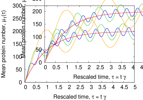
Figure 1: (Color online) Mean molecule number $\kappa_{1}(\tau)=\mu_{1}(\tau)$ as given by Eq. (22) for $r=1$, as a function of dimensionless time variable $\tau=\gamma t$, for $\kappa_{1}(0)=0$, $\varphi=0$, $\gamma=4\cdot 10^{-4}$ s, $m_{1}$ and $m_{2}$ given by (27), $a=10$, $b=20$, $C_{2}=a\gamma$, $C_{1}=C_{2}$ or $C_{1}=0$, and $T\gamma=\frac{1}{2}$ (blue), $T\gamma=1$ (green), $T\gamma=2$ (orange), and $C_{1}=0$ (time-independent $k(t)$, red curve).

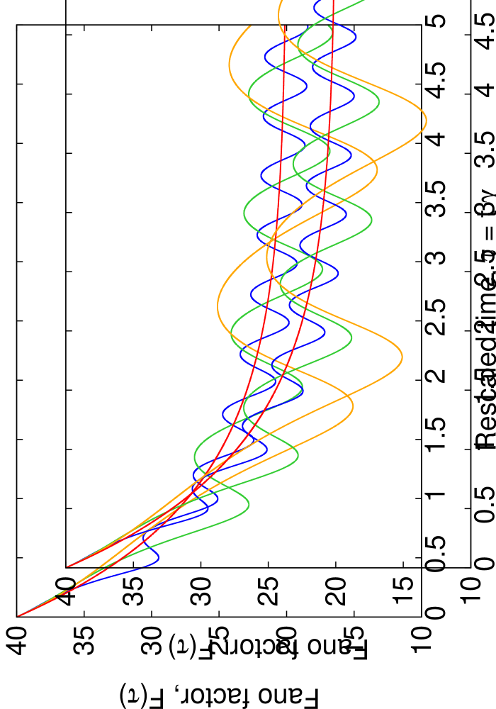
Figure 2: (Color online) Fano factor $F(\tau)=\kappa_{2}(\tau)/\kappa_{1}(\tau)$ as a function of dimensionless time variable $\tau=\gamma t$, for $\kappa_{1}(0)=\kappa_{2}(0)=0$, $\varphi=0$, $\gamma=4\cdot 10^{-4}$ s, $m_{1}$ and $m_{2}$ given by (27), $a=10$, $b=20$, $C_{2}=a\gamma$, $C_{1}=C_{2}$ or $C_{1}=0$, and $T\gamma=\frac{1}{2}$ (blue), $T\gamma=1$ (green), $T\gamma=2$ (orange), and $C_{1}=0$ (time-independent $k(t)$, red curve).

In Fig. 1 we plot the time evolution of the average protein number $\kappa_{1}(\tau)=\mu_{1}(\tau)$ as a function of dimensionless time variable $\tau=\gamma t$ and for various oscillation frequencies corresponding to $T\gamma=\frac{1}{2}$ (blue), $T\gamma=1$ (green) and $T\gamma=2$ (orange), as well as for the limiting case of nonoscillatory driving ($C_{1}=0$). We assume that $p(x,0)=\delta(x)$, therefore $\kappa_{1}(0)=\kappa_{2}(0)=0$. Also, we assume here that $\nu(u)$ is an exponential distribution (subscript $\epsilon$ stands for ’exponential’)

$$\nu_{\epsilon}(u)=\frac{1}{b}\exp\left(-\frac{u}{b}\right).$$ (25)

Moments of $\nu_{\epsilon}(u)$ (25) are given by

$$m^{(\epsilon)}_{n}=b^{n}n!.$$ (26)

In particular, we have

$$m^{(\epsilon)}_{1}=b,~{}~{}~{}~{}m^{(\epsilon)}_{2}=2b^{2}.$$ (27)

Exponentially (or geometrically) distributed sizes of translational bursts have been observed in E. coli Cai et al. (2006); Yu et al. (2006); Taniguchi et al. (2010); Choi et al. (2008). For that reason, $\nu_{\epsilon}(u)$ (25) appears to be a natural choice of the burst size distribution in the case of stochastic models of gene expression in which particle concentration is used instead of discrete particle number. Note that any other choice of $\nu(u)$ can only affect values of $m_{1}$ and $m_{2}$ in Eq. (22); this results in identical rescaling of each plot along the $y$-axis. As can be inferred from Eq. (22), the amplitude of oscillation is the largest for the largest oscillation period.

Similarly, in Fig. 2 we plot the time evolution of the Fano factor $F(\tau)$ (19), again as a function of dimensionless time variable $\tau=\gamma t$ and for the same model parameters as in Fig 1. By employing the L’Hôpital’s rule, it can be shown that for $\kappa_{1}(0)=\kappa_{2}(0)=0$ and $\nu(u)=\nu_{\epsilon}(u)$ (25) we have

$$\lim_{\tau\to 0}F(\tau)=2b,$$ (28)

which is close to value ($F(0^{+})=2b+1$) obtained in Ref. (Thattai and Van Oudenaarden, 2001) for a similar discrete model.

Most of the results of the present Section can be immediately generalized to the case of arbitrary periodic dependence of burst frequency

$$k(t)=a^{(k)}_{0}+\sum_{q=1}^{\infty}\left[a^{(k)}_{q}\cos\left(q\omega_{f}t\right)+b^{(k)}_{q}\sin\left(q\omega_{f}t\right)\right].$$ (29)

Invoking (14), for $k(t)$ given by (29) we obtain

$$\kappa_{r}(t) = \mathcal{T}_{r}(t)+\mathcal{P}_{r}(t)+\frac{a^{(k)}_{0}m_{r}}{r\gamma},$$ (30)

where

$$\mathcal{T}_{r}(t) = \left(\kappa_{r}(0)+\sum_{q=0}^{\infty}\frac{b^{(k)}_{q}q\omega_{f}-a^{(k)}_{q}r\gamma}{r^{2}\gamma^{2}+q^{2}\omega^{2}_{f}}m_{r}\right)e^{-r\gamma t},$$

and

$$\mathcal{P}_{r}(t) = \sum_{q=1}^{\infty}a^{(k)}_{q}\left(\frac{q\omega_{f}\sin(q\omega_{f}t)+r\gamma\cos(q\omega_{f}t)}{r^{2}\gamma^{2}+q^{2}\omega^{2}_{f}}\right)m_{r}$$

$$+ \sum_{q=1}^{\infty}b^{(k)}_{q}\left(\frac{r\gamma\sin(q\omega_{f}t)-q\omega_{f}\cos(q\omega_{f}t)}{r^{2}\gamma^{2}+q^{2}\omega^{2}_{f}}\right)m_{r}.$$

In Appendix C we show that the division of $\kappa_{r}(t)$ into constant, transient and periodic part as given by (30) remains valid when not only $k(t)$, but also $\gamma(t)$ or $\nu(u,t)$ are periodic functions of time.

Finally, let us note that Eq. (17) with $k(t)$ given by (20) or, in general case, by (29) has a simple mechanical interpretation. Namely, it is the equation of motion of a particle moving with velocity $v=\kappa_{r}$ in a viscous medium under the influence of both the drag force ($-r\gamma\kappa_{r}(t)$, with constant $\gamma$) and the external periodic force $m_{r}(t)k(t)$. Perhaps an even more compelling analogy is the RC low-pass filter: Fast oscillations of the external driving of gene expression Mugler et al. (2010) have less effect than slow ones.

II.2 Time-independent model parameters

Time evolution of $p(x,t)$

When the model parameters do not depend on time, i.e., $k(t)=k$, $\gamma(t)=\gamma$, and $\hat{w}(s,t)=\hat{w}(s)$, Eq. (7) may be rewritten as

$$\hat{p}(s,t)=\Phi(s\Omega(t))\exp\left[a\Psi(s)-a\Psi(s\Omega(t))\right],$$ (33)

where

$$a=\frac{k}{\gamma},$$ (34)

$$\Psi(z)=\int\frac{\hat{w}(z)}{z}dz.$$ (35)

$\Phi(z)$ is given again by Eq. (8), whereas

$$\Omega(t)=\exp(-\gamma t)$$ (36)

is a special case of (9). In the steady-state limit, from (33) we obtain

$$\lim_{t\to\infty}\hat{p}(s,t)\equiv\hat{p}(s)=\exp\left[a\left(\Psi(s)-\Psi(0)\right)\right].$$ (37)

The form of stationary distribution $p(x)$ (we distinguish stationary and nonstationary probability distribution functions by the number of arguments) depends neither on the values of $k$ and $\gamma$ parameters alone, nor on the initial condition, but only on the functional form of the burst size pdf $\nu(u)$ and value of the parameter $a$ (34).

Using (37), we may rewrite (33) as

$$\hat{p}(s,t)=\Phi(s\Omega(t))[\hat{p}(s\Omega(t))]^{-1}\hat{p}(s).$$ (38)

Invoking the following property of Laplace transform Abramowitz and Stegun (1964)

$$\mathcal{L}^{-1}\left[\hat{f}(\alpha s)\right]=\frac{1}{\alpha}f\left(\frac{x}{\alpha}\right),$$ (39)

where $\hat{f}(s)=\mathcal{L}[f(x)]$, by taking the inverse Laplace transform of (38) we can express $p(x,t)$ as the convolution of three terms

$$p(x,t)=\frac{1}{\Omega(t)}p\left(\frac{x}{\Omega(t)},0\right)\ast p(x)\ast\frac{1}{\Omega(t)}q\left(\frac{x}{\Omega(t)}\right),$$ (40)

where

$$p(x)=\mathcal{L}^{-1}\left[\hat{p}(s)\right],~{}~{}~{}~{}q(x)=\mathcal{L}^{-1}\left[1/\hat{p}(s)\right].$$ (41)

$\hat{p}(s)$ (37) and $1/\hat{p}(s)$ cannot simultaneously satisfy the necessary conditions required for the Laplace transform of an ordinary function, in particular the condition $\lim_{s\to\infty}\hat{f}(s)=0$. Clearly, the latter condition should be obeyed by $\hat{p}(s)$, hence we have $\lim_{s\to\infty}(1/\hat{p}(s))=\infty$. This implies that $q(x)$ (41) is not an ordinary function, but a distribution consisting of (apart from some ordinary function) superposition of delta distribution and its derivatives. In particular, if $1/\hat{p}(s)$ is a polynomial of degree $M$,

$$\frac{1}{\hat{p}(s)}=\sum_{k=0}^{M}q_{k}s^{k},$$ (42)

we obtain

$$q(x)=\sum_{k=0}^{M}q_{k}\delta^{(k)}(x).$$ (43)

If the explicit form of both $p(x)$ and $q(x)$ (43) is known, it may be feasible to find the explicit form of $p(x,t)$ by invoking Eq. (40) and the identity

$$(\delta^{(k)}\ast f)(x)=f^{(k)}(x).$$ (44)

Derivative on the r.h.s of Eq. (44) should be understood as a distribution derivative Schwartz and Denise (1965). Namely, if $f(x)$ has a discontinuity at $x=0$, but is at least $m$ times differentiable for $x\neq 0$, the $m$-th distribution derivative of $f(x)$ reads

$$f^{(m)}=\{f^{(m)}\}+\sigma_{0}\delta^{(m-1)}+\sigma_{1}\delta^{(m-2)}+\ldots++\sigma_{m-1}\delta,$$ (45)

where $\{f^{(m)}\}$ denotes distribution related to $f^{(m)}$ treated as an ordinary function (not defined at $x=0$), whereas $\sigma_{k}=f^{(k)}(0^{+})-f^{(k)}(0^{-})$ Schwartz and Denise (1965). In Appendix F we apply Eqs. (38)-(45) to obtain solution of Eq. (4) with the exponential probability distribution of burst sizes (25) in an alternative way than the one used in Section II.3.

Time evolution of cumulants of $p(x,t)$

If the model parameters do not depend on time, Eq. (14) takes a remarkably simple form

$$\kappa_{r}(t)=\kappa_{r}(0)e^{-r\gamma t}+a\left(1-e^{-r\gamma t}\right)\frac{m_{r}}{r},$$ (46)

where $m_{r}$ is given by Eq. (15) with $\nu(u,t)=\nu(u)$. In the $t\to\infty$ limit, from (46) we obtain

$$\kappa_{r}=\kappa_{r}(\infty)=a\frac{m_{r}}{r}.$$ (47)

which also follows from Eq. (79) of Appendix D (in this Appendix, we further elaborate on the relationship between functional form of the burst size probability distribution $\nu(u)$ and the functional form of the corresponding steady-state distribution of protein concentration, $p(x)$). Using (47), we may rewrite (46) as

$$\kappa_{r}(t)=\kappa_{r}(0)e^{-r\gamma t}+\kappa_{r}(\infty)\left(1-e^{-r\gamma t}\right).$$ (48)

The time evolution of $\kappa_{r}(t)$ as given by (46) or (48) consists of the exponentially decaying contribution coming from the initial probability distribution $p(x,0)$, as well as the contribution proportional to the stationary distribution (47); the latter is completely determined solely by the values of $a$ and $m_{r}$.

In the present case, if only the initial distribution $p(x,0)$ is known, the time evolution of cumulants may be immediately recovered from (46) if needed. This allows us to concentrate solely on the stationary limit ($t\to\infty$). Next, by making use of (13) and (46), we can obtain $\hat{p}(s,t)$ in the form of a power series in $s$ variable.

From Eqs. (46) or (48) we see that the higher the cumulant order $r$ is, the faster $\kappa_{r}(t)$ approaches its stationary value. In particular, variance approaches stationary value faster than the mean protein concentration. For $r=1$, from (47) we obtain a simple relation,

$$\kappa_{1}=\mu_{1}=m_{1}a.$$ (49)

The parameter $a$ as defined by Eq. (34) is equal to the burst frequency, $k$, multiplied by the characteristic time scale of the system, $T_{\gamma}=1/\gamma$. Therefore $a$ is proportional to the mean number of bursts (in Ref. Friedman et al. (2006) parameter $a$ itself is called the burst frequency) and (49) has a simple interpretation, i.e., the average protein concentration (number) is the average burst size times the mean number of bursts in time interval of the length $1/\gamma$.

For $r=2$, Eq. (46) can be rewritten as

$$\kappa_{2}(t)=\kappa_{2}(0)e^{-2\gamma t}+\frac{a}{2}\left(1-e^{-2\gamma t}\right)\left(\sigma^{2}(u)+b^{2}\right),$$ (50)

where $m_{1}=b$ and $\sigma^{2}_{\nu}(u)=m_{2}-b^{2}$ is the variance of $\nu(u)$. The term proportional to $\sigma_{\nu}^{2}(u)$ in Eq. (50) is related to the stochasticity of the burst size distribution. However, even for the dispersionless ($\sigma_{\nu}(u)=0$) burst size distribution,

$$\nu_{\delta}(u)=\delta\left(u-{b}\right),$$ (51)

we have an irreducible contribution to $\kappa_{2}(t)$ coming from the term proportional to $b^{2}$ in Eq. (50). For a fixed $m_{1}=b$, $\nu_{\delta}(u)$ (51) minimizes the variance of $p(x,t)$, a result which could be intuitively expected.

II.3 Example: p(x,t) corresponding to the exponential burst size distribution

In this section we find the time-dependent solution of Eq. (4) for the exponential burst size distribution (25). Apart from gene expression models, exponential distribution (25), as well as closely related two-sided exponential distribution found applications in models of other phenomena Porporato and D’Odorico (2004); Daly and Porporato (2006, 2010); Suweis et al. (2011); Mau et al. (2014). It should be also noted that in most cases only for $\nu(u)$ of the form (25) both Eq. (4) and its generalizations (e.g., jump-diffusion equations Luczka et al. (1995); Czernik et al. (1997); Łuczka et al. (1997)) are analytically tractable.

As shown in Ref. Friedman et al. (2006), for the time-independent model parameters, $\nu_{\epsilon}(u)$ (25) leads to stationary distribution $p(x)$ in the form of gamma distribution,

$$q_{\gamma}(x;a,b)\equiv\frac{x^{a-1}e^{-\frac{x}{b}}}{b^{a}\Gamma(a)}=\mathcal{L}^{-1}\left[\frac{1}{(sb+1)^{a}}\right].$$ (52)

This can be readily verified by making use of Eqs. (35) and (37).

From (26) and (46) we have

$$\kappa^{(\epsilon)}_{n}(t)=\kappa_{n}(0)e^{-n\gamma t}+a\left(1-e^{-n\gamma t}\right)b^{n}(n-1)!$$ (53)

In the $t\to\infty$ limit, we obtain $\kappa^{(\epsilon)}_{n}=ab^{n}(n-1)!$, i.e., the cumulants of gamma distribution (52). From (13) and (53) the Taylor series expansion of $\ln[\hat{p}_{\epsilon}(s)]$ can be reconstructed, we get

$$\ln[\hat{p}_{\epsilon}(s)]=a\sum_{n=1}^{\infty}\frac{(-bs)^{n}}{n}=\ln\left[\frac{1}{(sb+1)^{a}}\right],$$ (54)

hence $\hat{p}_{\epsilon}(s)=(sb+1)^{-a}$, which is indeed the inverse Laplace transform of gamma distribution (52).

Interestingly, in the present case both the explicit expression for $\hat{p}_{\epsilon}(s,t)$ and even for $p_{\epsilon}(x,t)$ can be obtained, at least for the initial distribution of the form

$$p_{\epsilon}(x,0)=\delta(x-x_{0}),$$ (55)

where $x_{0}\geq 0$ is the initial molecule concentration. The Laplace transform of (55) is $\hat{p}_{\epsilon}(s,0)=\exp(-x_{0}s)$, and hence from (33) we obtain

$$\hat{p}_{\epsilon}(s,t) = \left(\frac{se^{-\gamma t}+\frac{1}{b}}{s+\frac{1}{b}}\right)^{a}\exp(-x_{0}e^{-\gamma t}s).$$ (56)

For simplicity, we put $x_{0}=0$ (which is arguably the most natural choice in the case of gene expression models). Moreover, we confine our attention to $a=n\in\mathbb{N}$, as only in this case we were able to find compact analytical expression for the inverse Laplace transform of $\hat{p}_{\epsilon}(s,t)$ (56). Still, (56) is valid for arbitrary real $a>0$. It is also convenient to change the independent variable according to $t\to\omega=\exp(-\gamma t)$. In such a case, $\tilde{p}_{\epsilon,n}(x,\omega(t))\equiv p_{\epsilon,n}(x,t)=\mathcal{L}^{-1}\{\hat{p}_{\epsilon,n}(s,t)\}$ reads

$$\tilde{p}_{\epsilon,n}(x,\omega) = \omega^{n}\delta(x)+\sum_{i=1}^{n}{{n}\choose{i}}\frac{(1-\omega)^{i}\omega^{n-i}}{(i-1)!b^{i}}x^{i-1}e^{-\frac{x}{b}}$$

$$\equiv \omega^{n}\delta(x)+\sum_{i=1}^{n}{{n}\choose{i}}(1-\omega)^{i}\omega^{n-i}q_{\gamma}(x;i,b),$$

where $q_{\gamma}(x;i,b)$ is given by (52), whereas by $\hat{p}_{\epsilon,n}(s,t)$ we denote $\hat{p}_{\epsilon}(s,t)$ (56) for $a=n$ and similarly for $p_{\epsilon,n}(x,t)$ and $\tilde{p}_{\epsilon,n}(x,\omega)$. Each of $\tilde{p}_{\epsilon,n}(x,\omega)$ functions (LABEL:solution_for_p_no_hat_x) for $n=1,2,\ldots$ is a superposition of gamma distributions (Dirac delta can be also treated as a limiting case of the gamma distribution) with different integer values of $a$ and time-dependent weights. Hence, (LABEL:solution_for_p_no_hat_x) is a natural time-dependent generalization of the gamma distribution (52) with $a=n$, obtained in Friedman et al. (2006), where only the stationary limit of Eq. (4) has been considered.

Note that for $x_{0}=0$, the dependence of $\hat{p}_{\epsilon}(s,t)$ (56) on $s$ and the mean burst size $b$ is of the form (92), therefore $p_{\epsilon}(x,t)=\mathcal{L}[\hat{p}_{\epsilon}(s,t)]$, and in particular $p_{\epsilon,n}(x,t)=\tilde{p}_{\epsilon,n}(x,\omega(t))$ (LABEL:solution_for_p_no_hat_x) have the characteristic dependence on $x$ variable and $b$ parameter as given by (93), cf. Appendix E.

An alternative way of obtaining $\tilde{p}_{\epsilon,n}(x,\omega)$ (LABEL:solution_for_p_no_hat_x), its generalization for $x_{0}>0$ and its explicit form for small $n$ are discussed in Appendix F.

III Discussion, biological insights

The stochastic description of the simple system studied here shares a common feature with the corresponding deterministic model: The time evolution of the average protein number predicted by the stochastic model is identical with the time evolution of the protein concentration obtained from deterministic equations of kinetics (see Appendix A). On the other hand, the evolution of the $n$-th cumulant of the protein number distribution in time depends solely on the behavior of the $n$-th moment of the burst size distribution in time, but it does not depend on its other moments. In consequence, the time evolution of the average molecule number is identical for all burst size distributions which have the same first moments, if only the remaining model parameters are identical. If additionally the time dependence of the second moments of the burst size distributions is identical, we obtain an identical time dependence of the coefficient of variation and the Fano factor of the protein number distributions, the two important measures of gene expression noise. And therefore, the predictions of stochastic models with bursty molecule production are, to a large extent, universal as they do not depend on other details of the burst statistics. This may explain the success of gene expression models that commonly assume exponentially distributed burst sizes, despite the fact that the experimental evidence for this particular burst size distribution can be found in only a few papers Cai et al. (2006); Yu et al. (2006); Taniguchi et al. (2010); Choi et al. (2008). (Note that a somewhat similar conclusion about an unexpected universality of coarse-grained models was drawn by Pedraza et al. Pedraza and Paulsson (2008) in regards to statistics of waiting times between mRNA bursts.)

It should also be noted that the effective bursty dynamics results from the approximation based on integrating out fast degrees of freedom. In order to check the range of validity of this approximation, the dynamics of the effective model (e.g. with protein but without mRNA, as considered here) should be compared with the dynamics of the full model including both slow (protein copy number) and fast (mRNA copy number) degrees of freedom. However, it is expected that predictions of the latter model are in agreement with the predictions of the former for $t$ greater than few mRNA lifetimes Thattai and Van Oudenaarden (2001); Shahrezaei and Swain (2008).

The Eq. (46) shows that the relaxation of the variance is twice faster than that of the mean (Fig. 3 A). This has been shown previously for the model of gene expression where mRNA was explicitly taken into account and all reactions were Poissonian Thattai and Van Oudenaarden (2001). The same has been shown in ref. Bar-Even et al. (2006) (supplementary information therein), without referring to any particular reaction statistics. Eq. (46), on the other hand, links that result with the moments of an arbitrary distribution of protein bursts. Below, we will discuss these results in the context of evolutionary optimization of biological processes with respect to time-dependent noise intensity, and also we will relate the behavior of Eq. (46) to experimentally measurable scaling relations between protein mean and variance. Although our model does not account for extrinsic noise nor feedback in gene regulation, our analysis may shed some light on understanding of the relation between protein number statistics and underlying burst statistics.

III.1 Optimization of protein level detection with respect to noise is dependent on the assumed measure of noise

Suppose that a cell population expresses a protein at a certain level in given environmental conditions, and then the conditions abruptly change, which results in a change in the expression level. How does the width of the protein distribution vary over time before it reaches a new steady state? Although the stationary behavior of noise in gene circuits has been widely studied, somewhat less studies have been devoted to transient behavior of noise (see e.g. Thattai and Van Oudenaarden (2001); Tabaka et al. (2008); Palani and Sarkar (2012); Dixon et al. (2016)).

The difference in relaxation time scales of the protein mean and variance may result in a nonmonotonic or, at least, nonlinear dependence of noise on time. It would be tempting to put forward a hypothesis that this feature may be exploited by evolution for optimization of some processes with respect to noise: For example, let the gene expression be reduced from an induced level to a basal level, and suppose that this reduction should trigger some other processes in the cell. For the trigger to be maximally precise (such that all cells can detect the decrease in protein concentration at almost the same time), its threshold should not necessarily be located precisely at the basal expression level, but perhaps somewhere higher, where the noise is minimal.

We will show below, however, that such interpretations are dependent on the function assumed to quantify noise. We do not know what measure of noise does the biological evolution use – that probably depends on the nature of a specific biological process. Coefficient of variation $\eta(t)$ (19) seems to be a relatively natural choice because it measures the ratio of distribution width to its mean, so it is a dimensionless quantity. However, Fano factor $F(t)$ (19) is also frequently used in literature, a function that measures the ratio of variance to the mean, i.e. the deviation of the process from Poissonian statistics. On the other hand, in the context of detection of transition between two expression levels, an equally natural choice may be the fractional change of the distribution width between the initial and final (stationary) state. One can easily see that each of these quantities behaves differently.

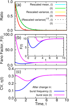
Figure 3: (Color online) Different measures of noise have a different transient behavior after an abrupt reduction of the mean burst frequency $a$ in a time unit defined by protein degradation (i), or the mean burst size $b$ (ii). The mean protein concentration $\langle x\rangle=ab$ was decreased from $10^{3}$ to $10^{2}$. A: Fractional change of mean, $K_{1}(t)$, fractional change of variance, $K_{2}(t)$, and its square root, $K_{2}(t)^{1/2}$. The curves for the cases (i) and (ii) overlap. B: Fano factor $F(t)$, inset: zoom to show the minima. C: Coefficient of variation, $\eta(t)$.

For visualization of the problem, suppose that the proteins are produced in exponential bursts of a mean size $b$. The number of proteins is therefore gamma-distributed with mean $ab$ and variance $ab^{2}$. Let the initial expression level be $\langle x(0)\rangle=\kappa_{1}(0)=10^{3}$ proteins, and after the abrupt environmental change it tends to $\langle x(\infty)\rangle=\kappa_{1}(\infty)=10^{2}$. Such a change can be attained by two mechanisms: Decreasing $a$ (frequency modulation, FM) or decreasing $b$ (amplitude modulation, AM). Experimental evidence suggests that cells are able to adjust both $a$ and $b$ Padovan-Merhar et al. (2015). For $a=100$ and $b=10$, a ten-fold decrease in $\langle x\rangle$ by changing $a\rightarrow a/10$ at fixed $b$ results in a ten-fold change in variance (i). The same decrease in mean protein concentration by changing $b\rightarrow b/10$ at fixed $a$ yields a change in variance by the factor of $100$ (ii).

In the case (i), the coefficient of variation has a deep minimum in $t=0$, and the Fano factor has a minimum at $t\neq 0$ (a relatively deep one, compared to the initial and final values). These dependencies are different in the case (ii): Here, the coefficient of variation has a shallow minimum at $t\neq 0$, and the Fano factor decreases almost monotonically by one order of magnitude, with a minimum that is insignificant compared to the total change of $F(t)$ (see Fig. 3 B, C).

The situation is still different if one takes into consideration the fractional change in the protein distribution width between the initial and final state. It immediately follows from Eq. (48) that the fractional change of the $r$-th moment,

$$K_{r}(t)\equiv\frac{\kappa_{r}(t)-\kappa_{r}(\infty)}{\kappa_{r}(0)-\kappa_{r}(\infty)}=e^{-r\gamma t}.$$ (58)

In particular, the square root of the fractional change of the variance is equal to the fractional change of the mean (Fig. 3). If $K_{2}(t)$ (or its increasing function) is used as the measure of the distribution width, then its minimal value is at $t=\infty$. And therefore, the optimization of the position of a detection threshold to minimize noise would be ambiguous, depending on a function chosen to quantify noise.

The above example shows that any biological hypotheses regarding the evolutionary optimization of some processes with respect to the amount of noise must assume that evolution has a specified method of measurement of that noise. If such optimizations really take place in nature, then it seems that the way how the evolution quantifies noise depends on a particular biological process. To date, it is not clear, however, which measure of noise is important in which process. This problem deserves a deepened experimental analysis.

III.2 Frequency modulation and amplitude modulation cause different scalings of protein number variance to mean

Experimental results suggest that cells can control gene expression levels both by adjusting the mean burst frequency $a$ (frequency modulation, FM) and the mean burst size $b$ (amplitude modulation, AM) Padovan-Merhar et al. (2015). With the Eq. (46) of our model, we can relate these two types of burst control to the scaling of mean and variance of protein distributions.

According to Eqs. (46) and (47), the scaling of the variance of the protein number distribution with the mean depends on three parameters that describe burst statistics: mean burst frequency $a$, mean burst size $m_{1}$, and the second moment of the burst size distribution, $m_{2}$. For simplicity of notation, in the following discussion we will denote by $const.$ a constant whose value is universal for a set of different genes or for a single gene in cells cultured in various conditions. If the protein number distributions produced by the studied genes obey the scaling $\sigma^{2}_{x}/\langle x\rangle=\kappa_{2}(\infty)/\kappa_{1}(\infty)=F(\infty)=const.$ (i), then the moments of the burst size distribution depend on each other so that $m_{2}/m_{1}=const.$ and the mean burst frequency $a$ can be arbitrary. On the other hand, if one observes the scaling $\sigma^{2}_{x}/\langle x\rangle^{2}=\eta^{2}(\infty)=const.$ (ii), then the three burst parameters depend on each other so that $m_{2}/(am_{1}^{2})=const.$

If additionally the burst size distribution is such that $m_{2}/m_{1}^{2}=\alpha=const.$, as in our examples in the main text and in the Appendix E ($\alpha=1$ for delta burst size distribution, $\alpha=2$ for exponential, and $\alpha=(1+\lambda)/\lambda$ for gamma distribution, with $\lambda$ defined in the Eq. 101), then $\sigma^{2}_{x}/\langle x\rangle=const.$ (i) implies that the mean burst size $m_{1}$ is universal, and the gene expression levels in the studied gene set, or in the set of conditions studied, are modulated by varying the mean burst frequency $a$ (FM). If, on the other hand, $\sigma^{2}_{x}/\langle x\rangle^{2}=const$ (ii), then the mean burst frequency $a$ is universal and the gene expression level is modulated by mean burst size $m_{1}$ (AM). This dependence of the variance-to-mean relationship on AM or FM has been known Hornung et al. (2012), but an explicit or implicit assumption was that the burst size distributions are exponential. Here, we show that this property also extends to a class of nonexponential distributions.

Scaling (i) was observed, e.g., in S. cerevisiae Bar-Even et al. (2006), where different promoters controlled transcription of their native proteins fused with GFP, under different environmental conditions. Assuming burst size distributions such that $m_{2}/m_{1}^{2}=\alpha$, would it be possible that the mean size of protein burst was the same in all these experiments and only the burst frequency varied? This could perhaps be conceivable, if the protein burst size were globally limited by the availability of translational machinery, or if the mRNA of different GFP fusions had simultaneously similar stability and similar translation rates, such that the average number of proteins produced from one mRNA molecule was the same regardless of the gene. The burst frequencies could differ from gene to gene depending on the on/off switching rates of different promoters.

However, we note that if the parameters of the burst size distribution are independent on time, then this fact imposes a particular form of scaling of the mean and variance of protein number distribution with time (46). In the Ref. Bar-Even et al. (2006), the authors observed that when the variance and mean were normalized with respect to the initial state, $\Delta\kappa_{r}(t)\equiv[\kappa_{r}(t)-\kappa_{r}(0)]/\kappa_{r}(0)$, then the normalized variance was proportional to the normalized mean even in the time-dependent case out of the stationary state. Although the authors supposed that their theoretical model explained this scaling, it does not seem to be the case. The equations for nonstationary mean and covariance proposed in Bar-Even et al. (2006) are fully consistent with the moment equations of our model and they imply that

$$\frac{\Delta\kappa_{2}(t)}{\Delta\kappa_{1}(t)}=\frac{\Delta\kappa_{2}(\infty)}{\Delta\kappa_{1}(\infty)}(1+e^{-\gamma t}).$$ (59)

The value in the braces changes from $2$ to $1$, so $\Delta\kappa_{2}(t)/\Delta\kappa_{1}(t)$ cannot be maintained constant in time within our model, if the parameters of the burst distribution are constant in time. What if they are time-dependent? Using Eq. 14, one can easily check that no simple substitution of exponential dependence of $\{m_{1},\ m_{2},\ k\}~{}\sim~{}\exp(-\gamma t)$ or $\sim~{}\exp(-2\gamma t)$ allows the function $\Delta\kappa_{2}(t)/\Delta\kappa_{1}(t)$ to lose the dependence on time. The problem with time-dependent scaling suggests that as simple a model as ours may not be suitable for description of the data presented in Bar-Even et al. (2006). This also suggests that more detailed studies are needed on time dependence of protein noise and its relation to the properties of burst statistics.

Scaling (ii) was observed, e.g., in E. coli and S. cerevisiae cultured in different conditions Salman et al. (2012). The GFP gene was inserted under the control of three different promoters in multiple-copy plasmids (5 or 15 copies), or integrated into the genome in a single copy. If the distributions of burst sizes were such that $m_{2}/m_{1}^{2}=\alpha$, would it be possible to explain this scaling behavior within our model? Gene expression level should be then modulated by the mean burst size, and the burst frequency should be universal. The quadratic scaling of mean vs. variance (Salman et al. (2012), Fig. 3 therein) can be fitted by a one-parameter parabola $A\langle x\rangle^{2}$. We note that the values of $A$ are different for the three different promoters. Within our model, this would mean that each promoter has its own characteristic frequency of bursting. This would sound reasonable if single gene copies were studied. However, in the experiments of Salman et al. (2012), the promoters were present in variable numbers of copies. The burst frequencies of the gene copies should then add up (see Eq. 83) and a single promoter should have a lower burst frequency than its multiple copies, unless there is some mechanism of dosage compensation in cells, which keeps the total burst frequency independent on the copy number of a given promoter. Moreover, the universal scaling of the full protein number distributions in Salman et al. (2012) was defined by a function $\varphi((x-\langle x\rangle)/\sigma)$ (where $\sigma$ denotes standard deviation), so, for example, gamma distribution produced by exponential bursts does not obey that scaling. Therefore, the validity of our model with time-independent parameters and the AM modulation of gene expression seems unlikely in the case of the data presented in Salman et al. (2012).

Yet, the above considerations based on our simple theory reveal that there are still unexplored problems in the field of stochastic gene expression: Are the distributions of protein burst sizes constant in time? Do they always belong to the wide class of those fulfilling $m_{2}/m_{1}^{2}=\alpha$, which includes the exponential distribution, commonly assumed in modeling? Under what biological conditions are the protein number distributions controlled by amplitude modulation of protein bursts or by frequency modulation (AM vs. FM)? Do these mechanisms undergo dosage compensation in the case of gene multiplication? The present discussion may be, therefore, an inspiration for a deepened experimental analysis of time dependence of protein number statistics on the underlying burst size statistics.

Appendix A Deterministic rate equation

The deterministic model of the reaction kinetics for the system described by Eq. (1) is given by the following rate equation

$$\dot{x} = c(t)-\gamma(t)x,$$ (60)

where $x\geq 0$ is the molecule concentration, $c(t)$ is the source intensity, whereas $\gamma(t)$ is the decay parameter; dot denotes the time derivative. Note that $c(t)$ describes a deterministic birth process, in contrast to the random source intensity $I(t)$ of the corresponding stochastic model (2). The solution to the Eq. (60) for $x(0)=x_{0}$ can be readily obtained:

$$x(t)=e^{-\int_{t_{0}}^{t}\gamma(t^{\prime})dt^{\prime}}\left[x_{0}+\int_{t_{0}}^{t}c(t^{\prime})e^{\int_{t_{0}}^{t^{\prime}}\gamma(\tilde{t})d\tilde{t}}dt^{\prime}\right].$$ (61)

The existence of the stationary solution to Eq. (60), as well as the possible oscillatory character of molecule concentration $x(t)$ depends on the functional form of $c(t)$ and $\gamma(t)$. Clearly, in the case of time independent model parameters, i.e., $c(t)=c$ and $\gamma(t)=\gamma$, the unique, stable stationary point of (60) is given by

$$x_{s}=\frac{c}{\gamma}.$$ (62)

Appendix B Time-evolution of the moments of p(x,t)

Multiplying Eq. (4) by $x^{r}$ and integrating such obtained equation, one gets the time evolution equation for the $r$-th moment of $p(x,t)$,

$$\mu_{r}(t)=\int_{0}^{\infty}x^{r}p(x,t)dx.$$ (63)

In the resulting time evolution equation for $\mu_{r}(t)$, the term derived from the first term on the r.h.s of Eq. (4) is readily integrated by parts, whereas in the term containing $\nu(x-x^{\prime},t)$ we have to change order of integration with respect to $x$ and $x^{\prime}$ as well as to change the independent variables according to $(x,x^{\prime})\to(u,x^{\prime})$, $u=x-x^{\prime}$, cf. Ref. Feng et al. (2012). In result, we get

$$\dot{\mu}_{r}(t)=-r\gamma(t)\mu_{r}(t)+k(t)\sum_{q=1}^{r}\binom{r}{q}\mu_{r-q}(t)m_{q}(t),$$ (64)

where $m_{r}(t)$ denotes $r$-th moment of the burst size distribution $\nu(u,t)$ as given by Eq. (15), i.e.,

$$m_{r}(t)=\int_{0}^{\infty}u^{r}\nu(u,t)du.$$ (65)

We assume here that the burst size pdf $\nu(u,t)$ is properly normalized and that the normalization is conserved during time evolution, i.e. $m_{0}(t)=1$, but we impose no other restrictions on the functional form of $\nu(u,t)$. On the other hand, the normalization of $p(x,t)$, i.e., the condition $\mu_{0}(t)=1$ follows immediately from Eq. (64). For $r=1$, Eq. (64) reads

$$\dot{\mu}_{1}(t)=k(t)m_{1}(t)-\gamma(t)\mu_{1}(t).$$ (66)

Eq. (66) is identical to Eq. (60) provided that we put $c(t)=k(t)m_{1}(t)$. In such a case, the time evolution of the average molecule number $\mu_{1}(t)$ is the same as the time evolution of molecule concentration $x(t)$ in the corresponding deterministic model (60); this is a general property of linear deterministic dynamical systems van Kampen (2007); McQuarrie (1967). Therefore, making use of Eq. (61), we may immediately write down the solution of Eq. (66)

$$\mu_{1}(t)=\Omega(t)\left[\mu_{1}(0)+\int_{t_{0}}^{t}\frac{k(t^{\prime})m_{1}(t^{\prime})}{\Omega(t^{\prime})}dt^{\prime}\right],$$ (67)

where $\Omega(t)$ is defined by Eq. (9), i.e.,

$$\Omega(t)=\exp\left(-\int_{t_{0}}^{t}\gamma(t^{\prime})dt^{\prime}\right).$$ (68)

For each $n\in\mathbb{N}$, Eqs. (64) with $r=1,2,\ldots,n$ form closed hierarchy of linear differential equations (time evolution equation for $\mu_{r}(t)$ does not depend on $\mu_{i}(t)$ if $i>r$). Therefore, in principle, starting from $r=1$, the explicit analytical formula for $\mu_{n}(t)$ can be found iteratively for arbitrary $n$.

Appendix C Periodic time dependence of the model parameters

Below, we show that the possibility of division of $\kappa_{r}(t)$ into two parts, the exponentially decaying and periodic one, as demonstrated on the simple example analyzed in Subsection II.1, is in fact a general feature of the present model when its parameters depend periodically on time. We assume now that not only $k(t)$ (29), but also $\gamma(t)$, and $m_{r}(t)$ appearing in (14) are periodic functions of time (including constant function as the special case),

$$\gamma(t) = \sum_{q=0}^{\infty}\left[a^{(\gamma)}_{q}\cos\left(q\omega_{f}t\right)+b^{(\gamma)}_{q}\sin\left(q\omega_{f}t\right)\right],$$

$$m_{n}(t) = \sum_{q=0}^{\infty}\left[a^{(m)}_{n,q}\cos\left(q\omega_{f}t\right)+b^{(m)}_{n,q}\sin\left(q\omega_{f}t\right)\right],$$

where $\omega_{f}$ is given by Eq. (21). We also assume that at least one of $k(t)$, $\gamma(t)$, and $m_{n}(t)$ functions is nontrivial periodic function (i.e., is not a constant, $k(t)\gamma(t)m_{n}(t)\neq\text{const}$). From (LABEL:fourier_series_gamma) we obtain

$$\int_{t_{0}}^{t}\gamma(t^{\prime})dt^{\prime} = \sum_{q=1}^{\infty}\frac{1}{q\omega_{f}}\left[a^{(\gamma)}_{q}\sin\left(q\omega_{f}t\right)-b^{(\gamma)}_{q}\cos\left(q\omega_{f}t\right)\right]$$ (71)

$$- \mathcal{A}^{(\gamma)}_{0}+a^{(\gamma)}_{0}t,$$

where

$$\mathcal{A}^{(\gamma)}_{0} = a^{(\gamma)}_{0}t_{0}+\sum_{q=1}^{\infty}\frac{1}{q\omega_{f}}a^{(\gamma)}_{q}\sin\left(q\omega_{f}t_{0}\right)$$ (72)

$$- \sum_{q=1}^{\infty}\frac{1}{q\omega_{f}}b^{(\gamma)}_{q}\cos\left(q\omega_{f}t_{0}\right).$$

From (71) and (72) it follows that $[\Omega(t)]^{-r}$ can be written as

$$[\Omega(t)]^{-r}=e^{ra^{(\gamma)}_{0}t}\mathcal{P}_{1}(t)$$ (73)

where $\mathcal{P}_{1}(t)$ is a periodic function of time and $\Omega(t)$ is given by (9) or (68). From (73) it follows that the integrand appearing in Eq. (14), i.e., $k(t)m_{r}(t)/\left[\Omega(t)\right]^{r}$ is also of the form (73) but with $\mathcal{P}_{1}(t)$ replaced by another periodic function, $\mathcal{P}_{2}(t)=\mathcal{P}_{1}(t)k(t)m_{r}(t)$ (product of finite number of periodic functions is a periodic function itself). Next, consider the integral

$$\mathcal{I} = \int_{t_{0}}^{t}e^{ra^{(\gamma)}_{0}t^{\prime}}\mathcal{P}_{2}(t^{\prime})dt^{\prime}.$$ (74)

Because $\mathcal{P}_{2}(t^{\prime})$ can be expanded in a Fourier series, we are left with integrals of the form

$$\mathcal{I}_{s}(q) = \int_{t_{0}}^{t}e^{ra^{(\gamma)}_{0}t^{\prime}}\sin(q\omega_{f}t^{\prime})dt^{\prime}.$$ (75)

$$\mathcal{I}_{c}(q) = \int_{t_{0}}^{t}e^{ra^{(\gamma)}_{0}t^{\prime}}\cos(q\omega_{f}t^{\prime})dt^{\prime}.$$ (76)

The integrals (75) and (76) are elementary, we have

$$\int e^{\lambda t}\sin(\alpha t)dt=\frac{\lambda\sin(\alpha t)-\alpha\cos(\alpha t)}{\alpha^{2}+\lambda^{2}}e^{\lambda t}$$ (77)

and

$$\int e^{\lambda t}\cos(\alpha t)dt=\frac{\lambda\cos(\alpha t)+\alpha\sin(\alpha t)}{\alpha^{2}+\lambda^{2}}e^{\lambda t},$$ (78)

i.e., indefinite integral of the type (75) or (76) is a product of the exponential function and the periodic part containing $\sin(\alpha t)$ and $\cos(\alpha t)$ terms; definite integrals (75) and (76) contain also the constant (time-independent) part.

In result, the exponential term $e^{-ra^{(\gamma)}_{0}t}$ coming from $\left[\Omega(t)\right]^{r}$ in front of the integral in Eq. (14) cancels the corresponding exponential term $e^{ra^{(\gamma)}_{0}t}$ appearing in some (but not all) terms of definite integral (74); such terms depend on $t$ in a periodic manner. On the other hand, the remaining terms in Eq. (14) are not periodic, but exponentially decaying functions of time.

Appendix D Infinite divisibility property of protein concentration probability distribution

Equations (35) and (37) establish a mapping between $\hat{p}(s)=\hat{p}(s;a)$ and $\hat{\nu}(s)$, or, equivalently, between $p(x;a)$ and $\nu(u)$ (here we explicitly denote the dependence of probability distributions on the parameter $a$ both in $x$ and $s$ space). Given a particular stationary distribution of molecule concentration $p(x;a)$, we may ask what is the functional form of $\nu(u)$ for which $p(x;a)$ is a stationary solution of Eq. (4). From Eq. (33) we obtain

$$\hat{\nu}(s) = \frac{s}{a}\frac{\hat{p}^{\prime}(s;a)}{\hat{p}(s;a)}+1=\frac{s}{a}\left(\ln[\hat{p}(s;a)]\right)^{\prime}+1,$$ (79)

where prime denotes derivative with respect to $s$. Because $\hat{\nu}(s)$ is the Laplace transform of probability density function, for real $s\geq 0$ it must fulfill the following conditions: (i) $\hat{\nu}(0)=1$, (ii) $\hat{\nu}(s)\geq 0$ (iii) $\hat{\nu}^{\prime}(s)<0$, and (iv) $\lim_{s\to\infty}\hat{\nu}(s)=0$. This imposes restrictions on the allowed form of $\hat{p}(s;a)$; otherwise the solution of Eq. (79) satisfying (i)-(iv) may not exist. The condition (i) is fulfilled by arbitrary $\hat{p}(s;a)$, but conditions (ii), (iii) and (iv) involve parameter $a$. However, the dependence of any stationary solution $\hat{p}(s;a)$ of Eq. (6) on $a$ is of a special form; from (37) we have

$$\hat{p}(s;a)=\left[\hat{p}(s;1)\right]^{a},$$ (80)

where

$$\hat{p}(s;1)=\exp[\Psi(s)-\Psi(0)]$$ (81)

does not depend on $a$. Invoking (80) and (81), Eq. (79) can be rewritten as

$$\hat{\nu}(s)=s\frac{\hat{p}^{\prime}(s;1)}{\hat{p}(s;1)}+1.$$ (82)

The special form (80) of $\hat{p}(s;a)$ is a manifestation of the infinite divisibility property of stationary solutions of the present model. Equation (80) can be inferred even without solving Eq. (6). Namely, within the present model, a single gene with burst frequency $k$ is equivalent to (and can be replaced with) $N$ parallel, independent gene copies (sources) characterized by burst frequencies $k_{1},k_{2},\ldots,k_{N}$, provided that

$$k_{1}+k_{2}+\ldots+k_{N}=k,$$ (83)

(i.e., under the assumption that there is no additional mechanism of dosage compensation in cells which would decrease the burst frequency as the gene copy number increases) and that the burst size distributions are identical for each source,

$$\nu_{1}(u)=\nu_{2}(u)=\ldots=\nu_{N}(u)=\nu(u).$$ (84)

Each of these $N$ independent gene copies alone generates probability distribution $p_{i}(x_{i};a_{i})$ of a random variable $x_{i}$, $i=1,2,\ldots,N$, where $a_{i}=k_{i}/\gamma$, with $\gamma$ being a degradation constant, common for all molecules present in the system. We also have $a=a_{1}+a_{2}+\dots+a_{N}$. If all $N$ gene copies are simultaneously present, the total molecule concentration, $x=x_{1}+x_{2}+\dots+x_{N}$ is a sum of $N$ independent random variables $x_{i}$, and hence $p(x;a)$ is a convolution of $p_{1}(x_{1};a_{1}),p_{2}(x_{2};a_{2}),\ldots,p_{N}(x_{N};a_{N})$,

$$p(x;a)=p_{1}(x;a_{1})\ast p_{2}(x;a_{2})\ast\cdots\ast p_{N}(x;a_{N}).$$ (85)

In consequence, we have

$$\hat{p}(s;a)=\mathcal{L}[p(x;a)]=\hat{p}_{1}(s;a_{1})\hat{p}_{2}(s;a_{1})\cdots\hat{p}_{N}(s;a_{1}).$$ (86)

In particular, for $a_{1}=a_{2}=\ldots=a_{N}=a/N$ we have $\hat{p}_{1}(s;a/N)=\hat{p}_{2}(s;a/N)=\hat{p}_{N}(s;a/N)$, therefore

$$\hat{p}(s;a)=\hat{p}(s;a/N)^{N}.$$ (87)

Clearly, $\hat{p}(s;a)$ (80) is the solution of the above functional equation.

For the initial condition of the form $p(x,t_{0})=\delta(x)$ ($\Phi(z)=1$), probability distribution of the molecule concentration exhibits the infinite divisibility property not only in the $t\to\infty$ limit, but for arbitrary $t\geq t_{0}$ as well. Indeed, in such a case (38) reads

$$\hat{p}(s,t)=\frac{\hat{p}(s;a)}{\hat{p}(s\Omega(t);a)}=\left(\frac{\hat{p}(s;1)}{\hat{p}(s\Omega(t);1)}\right)^{a}.$$ (88)

From Eq. (88) we see that for $a=n\in\mathbb{N}$, $p(x,t;n)$ can be obtained as $n$-th convolution of $p(x,t;1)$,

$$p(x,t;n)=\underbrace{p(x,t;1)\ast\cdots\ast p(x,t;1)}_{\text{$n$~{}times.}}$$ (89)

From the above it follows that the property of infinite divisibility also works for the time-dependent distributions generated by our model, as long as the initial condition is given by delta function.

Appendix E Examples of burst size probability distributions

Below we analyze some properties of the solutions of Eq. (4), obtained for two selected choices of the burst size pdf $\nu(u)$.

First, we analyze an example of a simple burst size pdf in the form of Dirac delta distribution. In this case, as well as for all burst pdfs of the form $\nu(u)=\nu(u;b)$, i.e., depending on a single parameter $b$, equal to mean burst size, we obtain a two-parameter family of probability distributions of molecule concentration $p(x,t)=p(x,t;a,b)$. Next, we analyze the three-parameter family of probability distributions $p(x,t)=p(x,t;a,\lambda,\xi)$ obtained for the burst size distribution given by gamma distribution with parameters $\lambda$ and $\xi$. In order to compare this case with the remaining ones (Dirac delta and exponential distribution analysed in Section II.3), we put $\lambda\xi=b$. Therefore for all burst size distributions considered in the present paper, all moments $m_{n}$, $n=1,2,3,\dots$ are finite and $m_{1}=b$. Also, in each case analyzed here, the dependence of burst size probability distribution on burst size $u$ and mean burst size $b$ is of the form

$$\nu(u;b)=\frac{1}{b}h\left(\frac{u}{b}\right),$$ (90)

where $h(y)\geq 0$ and $\int_{0}^{\infty}h(y)dy=1$. For any $\nu(u;b)$ of the form (90), from (39) it follows that

$$\hat{\nu}(s;b)=\mathcal{L}\left[\nu(u;b)\right]=\hat{h}(sb)$$ (91)

where $\hat{h}(s)=\mathcal{L}[h(u)]$. From (91), (35), (37), and (38) it follows, that for $\Phi(s)=1$, we also have

$$\hat{p}(s,t;b,\ldots)=\hat{g}\left(sb,t;\ldots\right).$$ (92)

Therefore, for the initial distribution $p(x,t_{0})=\delta(x)$, the property (90) is inherited by $p(x,t)$, i.e., the dependence of the latter distribution on parameter $b$ is of the form

$$p(x,t;b,\ldots)=\frac{1}{b}g\left(\frac{x}{b},t;\ldots\right),$$ (93)

where by $\ldots$ we denote the remaining model parameters. Obviously, from (93) it follows that the corresponding stationary distribution of protein concentration depends on $b$ in the same manner,

$$p(x;b,\ldots)=\frac{1}{b}g\left(\frac{x}{b};\ldots\right).$$ (94)

E.1 Dirac delta distribution

The simplest form of the burst-size probability distribution $\nu(u)$ is the dispersionless delta distribution $\nu_{\delta}(u)$, Eq. (51), which describes identical bursts of size $b$. For this particular burst-size probability distribution, only the random distribution of the burst arrival times contributes to the stochastic character of the protein production, but there is no contribution of the burst-size fluctuations. Obviously, we have

$$m^{(\delta)}_{n}=b^{n}.$$ (95)

From (46), (47), and (95) we obtain now

$$\kappa^{(\delta)}_{n}(t)=\kappa_{n}(0)e^{-n\gamma t}+a\left(1-e^{-n\gamma t}\right)\frac{b^{n}}{n},$$ (96)

$$\kappa^{(\delta)}_{n}(\infty)=a\frac{b^{n}}{n}.$$ (97)

Equations (97) and (13) allow us to find Taylor series expansion of $\ln[\hat{p}_{\delta}(s)]$,

$$\ln[\hat{p}_{\delta}(s)]=a\sum_{n=1}^{\infty}\frac{(-bs)^{n}}{n!n}=-a\text{Ein}(-bs),$$ (98)

where

$$\text{Ein}(z) = \int_{0}^{z}\left(1-e^{-t}\right)\frac{dt}{t}=\sum_{k=1}^{\infty}\frac{(-1)^{k+1}z^{k}}{k~{}k!}$$ (99)

is related to exponential integral $\text{Ei}(z)$ in the following way Abramowitz and Stegun (1964)

$$\text{Ein}(-y)=-\text{Ei}(y)+\ln(y)+C_{\gamma},~{}~{}~{}~{}y>0.$$ (100)

In Eq. (100), by $C_{\gamma}$ we denote the Euler-Mascheroni constant, usually denoted by $\gamma$.

E.2 Gamma distribution

As a second example, we consider the case of burst size pdf $\nu(u)$ given by gamma distribution

$$\nu_{\gamma}(u;\lambda,\xi)=\frac{u^{\lambda-1}}{\xi^{\lambda}\Gamma(\lambda)}\exp\left(-\frac{u}{\xi}\right).$$ (101)

$\nu_{\gamma}(u;\lambda,\xi)$ (101) is one of the simplest continuous and differentiable unimodal burst size distribution functions. Moreover, burst size distributions similar to (101) appear naturally in certain models of gene expression Schwabe et al. (2012). This burst size distribution has also been analyzed in Ref. Daly and Porporato (2010). In order to compare $\nu_{\gamma}(u)$ with burst size distribution analyzed above, we put $\lambda\xi=m^{(\gamma)}_{1}=b$. Using the formula for $n$-th moment of gamma distribution

$$m^{(\gamma)}_{n}=\frac{\Gamma(n+\lambda)}{\Gamma(\lambda)}\xi^{n}=\frac{\Gamma(n+\lambda)}{\lambda^{n}\Gamma(\lambda)}{b}^{n},$$ (102)

and Eq. (47) we obtain

$$\kappa^{(\gamma)}_{n}=a\frac{\Gamma(n+\lambda)}{n\Gamma(\lambda)}\xi^{n}.$$ (103)

From (13) and (103) we obtain

$$\ln[\hat{p}_{\gamma}(s)]=a\sum_{n=1}^{\infty}\frac{\Gamma(n+\lambda)}{\Gamma(\lambda)\Gamma(n+1)}\frac{(-\xi s)^{n}}{n}.$$ (104)

Full time evolution of $\hat{p}_{\gamma}(s,t)$ can be easily recovered, if necessary. Further simplification are possible for $\lambda\in\mathbb{N}$. In such a case, instead of $s$ it is more convenient to use $\chi(s)=(sb+1)^{-1}$ as an independent variable. Because $\mathcal{L}^{-1}[(sb+1)^{-a}]=q_{\gamma}(x;a,b)$, cf. Eq. (52), the expansion of $\hat{p}_{\gamma}(s(\chi))$ in powers $\chi$ is equivalent with expressing $p(x)$ as a superposition of gamma distributions (52) with different values of $a$ but the same $b$. This ’gamma representation’ may be viewed in analogy with widely used Poisson representation Gardiner (2009).

In particular, for $\lambda=2$ the explicit formula for $p(x)$ can be obtained, we get

$$p_{\gamma}(x;2,\xi,a)=\frac{1}{(ea)^{a}}\frac{e^{-\frac{x}{\xi}}}{x}\mathcal{F}_{a}\left(\frac{x}{\xi}\right),$$ (105)

where

$$\mathcal{F}_{a}\left(y\right)=\frac{\left(ay\right)^{a}}{\Gamma(a)}+\left(ay\right)^{\frac{a+1}{2}}I_{a-1}\left(2\sqrt{ay}\right)$$ (106)

and $I_{\alpha}(z)$ is a modified Bessel function. Although (105) has a rather complicated form, it has a simple expansion in terms of gamma distributions (52), namely

$$p_{\gamma}(x;2,\xi,a)=\frac{1}{e^{a}}\sum_{n=0}^{\infty}\frac{a^{n}}{n!}q_{\gamma}(x;n+a,\xi).$$ (107)

Appendix F Alternative way of obtaining the solution for exponential burst size distribution function analysed in Section II.3 and some of its properties

The most convenient way to compute the inverse Laplace transform of $\hat{p}_{\epsilon}(s,t)$ (56) for $a=n\in\mathbb{N}$ is to rewrite $\hat{p}_{\epsilon}(s,t)=\hat{p}_{\epsilon,n}(s,t)$ as the following function of $\omega=e^{-\gamma t}$

$$\hat{p}_{\epsilon,n}(s,t) = \hat{\tilde{p}}_{\epsilon,n}(s,\omega)=\left(\omega+\frac{1-\omega}{sb+1}\right)^{n}e^{-x_{0}\omega s}$$ (108)

$$= \sum_{i=0}^{n}{{n}\choose{i}}\frac{(1-\omega)^{i}\omega^{n-i}}{(sb+1)^{i}}e^{-x_{0}\omega s}.$$

According to Eq. (52), the inverse Laplace transform of $(sb+1)^{-i}$ is a gamma distribution with parameters $i$ and $b$, whereas the the inverse Laplace transform of unity is a Dirac delta function. Hence, for $x_{0}=0$, from (108) we immediately obtain Eq. (LABEL:solution_for_p_no_hat_x). If $x_{0}\geq 0$, instead of $\tilde{p}_{\epsilon,n}(x,\omega)$ (LABEL:solution_for_p_no_hat_x) we obtain the more general solution $\tilde{p}_{\epsilon,n}(x,\omega;x_{0})$. From the well-known properties of Laplace transform it follows that $\tilde{p}_{\epsilon,n}(x,\omega;x_{0})$ has identical functional form as $\tilde{p}_{\epsilon,n}(x,\omega)$ (LABEL:solution_for_p_no_hat_x), but the $x$ variable is replaced by $\xi=x-x_{0}\omega$, i.e, $\tilde{p}_{\epsilon,n}(x,\omega;x_{0})=\tilde{p}_{\epsilon,n}(x-x_{0}\omega,\omega)$.

The explicit form of $\tilde{p}_{\epsilon,n}(x,\omega)$ (LABEL:solution_for_p_no_hat_x) can be also obtained in an alternative way. From Eq. (54) for $a=n\in\mathbb{N}$ and $e^{-\gamma t}=\omega$ we have

$$\frac{1}{\hat{p}(s\omega)}=\left(s\omega+\frac{1}{b}\right)^{n}=\omega^{n}\sum_{k=0}^{n}{n\choose k}\frac{s^{n-k}}{b^{k}\omega^{k}}.$$ (109)

By applying the inverse Laplace transform to (109), we obtain

$$\frac{1}{\omega}q\left(\frac{x}{\omega}\right)=\omega^{n}\sum_{k=0}^{n}{n\choose k}\frac{\delta^{(n-k)}(x)}{b^{k}\omega^{k}}.$$ (110)

For $x_{0}=0$, $\tilde{p}_{\epsilon,n}(x,\omega)$ is a convolution of $p(x)$ (52) and $q(x/\omega)/\omega$ (110), cf. Eq. (40). Invoking Eq. (44), we see that in order to obtain $\tilde{p}_{\epsilon,n}(x,\omega)$ we need to compute derivatives of $p(x)$ (52). However, one has to remember, that $p(x)$ is in fact a distribution, equal to $\Theta(x)q_{\gamma}(x;a,b)$, and not just an ordinary function $q_{\gamma}(x;a,b)$ (here by $\Theta(x)$ we denote a Heaviside step function). Therefore, in order to compute the $m$-th derivative of $p(x)$, Eq. (45) should be invoked.

It is also convenient to rewrite Eq. (LABEL:solution_for_p_no_hat_x) in a more compact form

$$\tilde{p}_{\epsilon,n}(x,\omega) = \omega^{n}\delta(x)+\tilde{W}_{\epsilon,n}(x,\omega)e^{-\frac{x}{b}},$$ (111)

where

$$\tilde{W}_{\epsilon,n}(x,\omega) = \sum_{i=1}^{n}{{n}\choose{i}}\frac{(1-\omega)^{i}\omega^{n-i}}{(i-1)!b^{i}}x^{i-1}.$$ (112)

Explicitly, for $n=0,1,2$ and $3$, we have

$$\tilde{W}_{\epsilon,0}(x,\omega) = 0,$$ (113)

$$\tilde{W}_{\epsilon,1}(x,\omega) = \frac{1-\omega}{b},$$ (114)

$$\tilde{W}_{\epsilon,2}(x,\omega) = \frac{(1-\omega)^{2}}{b^{2}}x+2\frac{(1-\omega)\omega}{b},$$ (115)

$$\tilde{W}_{\epsilon,3}(x,\omega) = \frac{(1-\omega)^{3}}{2b^{3}}x^{2}+3\frac{(1-\omega)^{2}\omega}{b^{2}}x$$ (116)

$$+ 3\frac{(1-\omega)\omega^{2}}{b}.$$

Clearly, $\tilde{p}_{\epsilon,n}(x,\omega)$ as given by (LABEL:solution_for_p_no_hat_x), (LABEL:solution_for_p_no_hat_x) or by Eqs. (113)-(116) has correct $\omega\to 1$ ($t\to 0$) and $\omega\to 0$ ($t\to\infty$) limits, as expected.

The validity of (LABEL:solution_for_p_no_hat_x) for each $n$ can also be verified directly by inserting $\tilde{p}_{\epsilon,n}(x,\omega)$ to Eq. (4). To deal with the term proportional to $\delta(x)$, one should invoke the identity $x\delta(x)\equiv 0$, in order to avoid differentiation of the distribution. Also, at $t=0$ ($\omega=1$), the initial condition (55) is satisfied, and in the $t\to\infty$ ($\omega\to 0$) limit, only the $i=n$ term of (LABEL:solution_for_p_no_hat_x) survives, leading again to gamma distribution (52). Also, it could be checked that $\tilde{p}_{n}(x,\omega)$ functions are correctly normalized for arbitrary $n$ and $\omega$. The weight of the $\delta(x)$ term, equal to $\omega^{n}$, vanishes more rapidly for larger values of $n$.

It can be also checked that $(\tilde{p}_{\epsilon,1}\ast\tilde{p}_{\epsilon,1})(x)=\tilde{p}_{\epsilon,2}(x)$, $(\tilde{p}_{\epsilon,1}\ast\tilde{p}_{\epsilon,2})(x)=\tilde{p}_{\epsilon,3}(x)$, etc., and that $\tilde{p}_{\epsilon,n}(x,\omega)$ (LABEL:solution_for_p_no_hat_x) is a $n$-fold convolution of $\tilde{p}_{\epsilon,1}(x)$, i.e., it obeys Eq. (89).

The $k$-th moment of the probability distribution $\tilde{p}_{n}(x,\omega)$ (LABEL:solution_for_p_no_hat_x) is equal to

$$\tilde{\mu}^{(\epsilon,n)}_{k}(\omega) \equiv \int^{\infty}_{0}x^{k}\tilde{p}_{\epsilon,n}(x,\omega)dx$$ (117)

$$= \sum_{i=1}^{n}A^{(n)}_{i}b^{k+i}\Gamma(k+i),$$

where

$$A^{(n)}_{i}\equiv{{n}\choose{i}}\frac{(1-\omega)^{i}\omega^{n-i}}{(i-1)!b^{i}}$$ (118)

In particular, we obtain

$$\tilde{\mu}^{(\epsilon,n)}_{1} = nb(1-\omega),$$

$$\tilde{\mu}^{(\epsilon,n)}_{2}-\left(\tilde{\mu}^{(\epsilon,n)}_{1}\right)^{2} = nb^{2}(1-\omega^{2})$$ (119)

$$= \tilde{\mu}^{(\epsilon,n)}_{1}b(1+\omega),$$

in agreement with Eq. (53). Note that the expression for $\tilde{\mu}^{(\epsilon,n)}_{1}$ obtained here is identical to that obtained in Ref. Shahrezaei and Swain (2008) within the corresponding discrete model, whereas the expressions for the variance differ, although the difference is small if only $b\gg 1$.

References

- Golding et al. (2005) I. Golding, J. Paulsson, S. M. Zawilski, and E. C. Cox, Cell 123, 1025 (2005).
- Ozbudak et al. (2002) E. M. Ozbudak, M. Thattai, I. Kurtser, A. D. Grossman, and A. van Oudenaarden, Nature Genetics 31, 69 (2002).
- Cai et al. (2006) L. Cai, N. Friedman, and X. Xie, Nature 440, 358 (2006).
- Yu et al. (2006) J. Yu, J. Xiao, X. Ren, K. Lao, and X. S. Xie, Science 311, 1600 (2006).
- Taniguchi et al. (2010) Y. Taniguchi, P. J. Choi, G.-W. Li, H. Chen, M. Babu, J. Hearn, A. Emili, and X. S. Xie, Science 329, 533 (2010).
- Choi et al. (2008) P. J. Choi, L. Cai, K. Frieda, and X. S. Xie, Science 322, 442 (2008).
- Friedman et al. (2006) N. Friedman, L. Cai, and X. S. Xie, Physical Review Letters 97, 168302 (2006).
- Shahrezaei and Swain (2008) V. Shahrezaei and P. S. Swain, Proceedings of the National Academy of Sciences 105, 17256 (2008).
- Paulsson and Ehrenberg (2000) J. Paulsson and M. Ehrenberg, Physical Review Letters 84, 5447 (2000).
- Aquino et al. (2012) T. Aquino, E. Abranches, and A. Nunes, Physical Review E 85, 061913 (2012).
- Lin and Galla (2016) Y. T. Lin and T. Galla, Journal of The Royal Society Interface 13, 20150772 (2016).
- Schwabe et al. (2012) A. Schwabe, K. N. Rybakova, and F. J. Bruggeman, Biophysical Journal 103, 1152 (2012).
- Elgart et al. (2011) V. Elgart, T. Jia, A. T. Fenley, and R. Kulkarni, Physical Biology 8, 046001 (2011).
- Kuwahara et al. (2015) H. Kuwahara, S. T. Arold, and X. Gao, Integrative Biology 7, 1622 (2015).
- Iyer-Biswas et al. (2009) S. Iyer-Biswas, F. Hayot, and C. Jayaprakash, Physical Review E 79, 031911 (2009).
- Tabaka and Hołyst (2010) M. Tabaka and R. Hołyst, Physical Review E 82, 052902 (2010).
- Ramos et al. (2011) A. F. Ramos, G. C. P. Innocentini, and J. E. M. Hornos, Physical Review E 83, 062902 (2011).
- Feng et al. (2012) H. Feng, Z. Hensel, J. Xiao, and J. Wang, Physical Review E 85, 031904 (2012).
- Pendar et al. (2013) H. Pendar, T. Platini, and R. V. Kulkarni, Physical Review E 87, 042720 (2013).
- Kumar et al. (2014) N. Kumar, T. Platini, and R. V. Kulkarni, Physical Review Letters 113, 268105 (2014).
- Mugler et al. (2010) A. Mugler, A. M. Walczak, and C. H. Wiggins, Physical Review Letters 105, 058101 (2010).
- Salman et al. (2012) H. Salman, N. Brenner, C.-k. Tung, N. Elyahu, E. Stolovicki, L. Moore, A. Libchaber, and E. Braun, Physical Review Letters 108, 238105 (2012).
- Bar-Even et al. (2006) A. Bar-Even, J. Paulsson, N. Maheshri, M. Carmi, E. O’Shea, Y. Pilpel, and N. Barkai, Nature Genetics 38, 636 (2006).
- Cox and Isham (1986) D. Cox and V. Isham, Advances in Applied Probability , 558 (1986).
- Takacs et al. (1961) L. Takacs et al., in Proc. Fourth Berkeley Symp. Math. Statist. Prob, Vol. 2 (1961) pp. 535–567.
- Luczka et al. (1995) J. Luczka, R. Bartussek, and P. Hänggi, EPL (Europhysics Letters) 31, 431 (1995).
- Czernik et al. (1997) T. Czernik, J. Kula, J. Łuczka, and P. Hänggi, Physical Review E 55, 4057 (1997).
- Łuczka et al. (1997) J. Łuczka, T. Czernik, and P. Hänggi, Physical Review E 56, 3968 (1997).
- Porporato and D’Odorico (2004) A. Porporato and P. D’Odorico, Physical Review Letters 92, 110601 (2004).
- Daly and Porporato (2006) E. Daly and A. Porporato, Physical Review E 73, 026108 (2006).
- Daly and Porporato (2010) E. Daly and A. Porporato, Physical Review E 81, 061133 (2010).
- Suweis et al. (2011) S. Suweis, A. Porporato, A. Rinaldo, and A. Maritan, Physical Review E 83, 061119 (2011).
- Mau et al. (2014) Y. Mau, X. Feng, and A. Porporato, Physical Review E 90, 052128 (2014).
- Perona et al. (2012) P. Perona, E. Daly, B. Crouzy, and A. Porporato, in Proc. R. Soc. A (The Royal Society, 2012) p. rspa20120396.
- Wheatland (2008) M. Wheatland, The Astrophysical Journal 679, 1621 (2008).
- Wheatland (2009) M. Wheatland, Solar Physics 255, 211 (2009).
- Askari and Krichene (2008) H. Askari and N. Krichene, Energy Economics 30, 2134 (2008).
- van Kampen (2007) N. van Kampen, Stochastic Processes in Physics and Chemistry, Elsevier Science (Amsterdam, 2007).
- Arfken et al. (2011) G. B. Arfken, H. J. Weber, and F. E. Harris, Mathematical methods for physicists: A comprehensive guide (Academic press, 2011).
- Gardiner (2009) C. Gardiner, Stochastic methods (Springer Berlin, 2009).
- Thattai and Van Oudenaarden (2001) M. Thattai and A. Van Oudenaarden, Proceedings of the National Academy of Sciences 98, 8614 (2001).
- Abramowitz and Stegun (1964) M. Abramowitz and I. A. Stegun, Handbook of mathematical functions: with formulas, graphs, and mathematical tables, Vol. 55 (Courier Corporation, 1964).
- Schwartz and Denise (1965) L. Schwartz and H. Denise, Methodes mathematiques pour les sciences physiques. (Hermann, Addison-Wesley Publishing Co., 1965).
- Pedraza and Paulsson (2008) J. M. Pedraza and J. Paulsson, Science 319, 339 (2008).
- Tabaka et al. (2008) M. Tabaka, O. Cybulski, and R. Hołyst, Journal of Molecular Biology 377, 1002 (2008).
- Palani and Sarkar (2012) S. Palani and C. A. Sarkar, Cell Reports 1, 215 (2012).
- Dixon et al. (2016) J. Dixon, A. Lindemann, and J. H. McCoy, Physical Review E 93, 012415 (2016).
- Padovan-Merhar et al. (2015) O. Padovan-Merhar, G. P. Nair, A. G. Biaesch, A. Mayer, S. Scarfone, S. W. Foley, A. R. Wu, L. S. Churchman, A. Singh, and A. Raj, Molecular Cell 58, 339 (2015).
- Hornung et al. (2012) G. Hornung, R. Bar-Ziv, D. Rosin, N. Tokuriki, D. S. Tawfik, M. Oren, and N. Barkai, Genome Research 22, 2409 (2012).
- McQuarrie (1967) D. A. McQuarrie, Journal of Applied Probability 4, 413 (1967).