Interplay between Rashba spin-orbit coupling and adiabatic rotation in a two-dimensional Fermi gas

Abstract

We explore the trap profiles of a two-dimensional atomic Fermi gas in the presence of a Rashba spin-orbit coupling and under an adiabatic rotation. We first consider a non-interacting gas and show that the competition between the effects of Rashba coupling on the local density of single-particle states and the Coriolis effects caused by rotation gives rise to a characteristic ring-shaped density profile that survives at experimentally-accessible temperatures. Furthermore, Rashba splitting of the Landau levels takes the density profiles on a ziggurat shape in the rapid-rotation limit. We then consider an interacting gas under the BCS mean-field approximation for local pairing, and study the pair-breaking mechanism that is induced by the Coriolis effects on superfluidity, where we calculate the critical rotation frequencies both for the onset of pair breaking and for the complete destruction of superfluidity in the system. In particular, by comparing the results of fully-quantum-mechanical Bogoliubov-de Gennes approach with those of semi-classical local-density approximation, we construct extensive phase diagrams for a wide-range of parameter regimes in the trap where the aforementioned competition may, e.g., favor an outer normal edge that is completely phase separated from the central superfluid core by vacuum.

I Introduction

Most of the exotic many-body phenomena observed in an atomic Fermi gas are triggered by a variety of couplings between single-particle states and externally-applied fields, and therefore, they relate directly to the single-particle properties of a normal (N) Fermi gas. For instance, appropriate couplings between the internal atomic degrees of freedom and laser fields have made it possible to create and engineer effective electromagnetic fields, i.e., artificial Abelian gauge fields, for neutral atoms Dalibard2011 . Alternatively, since the effects of rotation are analogous to those of an effective magnetic field on a particle, where the Coriolis force on a neutral atom mimics the Lorentz force on a charged particle, such a coupling may be used to form Landau levels in a trapped Fermi gas exhibiting an integer quantum-Hall effect Ho2000 . In addition, recent progress in creating effective spin-orbit couplings (SOC), i.e., artificial non-Abelian gauge fields, also opens the door for analogous cold-atom studies on quantum spin-Hall effect Sinova2004 ; Qi2011 and topological insulators Hasan2010 ; Qi2011 . Bringing such couplings together naturally generates further novel effects. For example, while the simultaneous presence of Rashba SOC and Zeeman field may give rise to an anomalous-Hall effect Zhang2010 , the interplay of Rashba coupling and adiabatic rotation may lead to the formation of a ring-shaped annulus in a trapped Fermi gas Doko2016 .

SOC and related contemporary phenomena have arisen as some of the key components in the interdisciplinary contexts of modern many-body quantum systems, including the cold atoms, and their understanding premise in the possibility of engineering cutting-edge technologies that are based on topological solid-state materials. In this respect, the experimental realizations of an effective SOC via artificial gauge fields Lin2011 ; Zhang2012 ; Wang2012 ; Cheuk2012 ; Qu2013 ; Goldman2014 ; Olson2014 , including the possibility of real-time control Jimenez-Garcia2015 , extend the stage to investigate SOC physics in experimentally-controllable settings. Even though early experimental works were limited to a one-dimensional SOC, which may be considered as an equal-weight combination of Rashba and Dresselhaus couplings, a two-dimensional SOC has recently been realized Huang2015 by using a three-laser Raman scheme, paving the way for the realization of a purely Rashba coupling. There are various other theoretical proposals that are based on magnetic or generalized Raman schemes for creating a Rashba coupling as well Ruseckas2005 ; Stanescu2007 ; Dalibard2010 ; Campbell2011 ; Xu2012 ; Anderson2013 ; Campbell2016 . Furthermore, motivated by the experimental realizations of a 2D Fermi gas Martiyanov2010 ; Dyke2011 ; Frohlich2011 ; Feld2011 ; Sommer2012 ; Ries2015 , the effects of SOC on a 2D Fermi gas have recently been the subject of many theoretical works Zhou2011a ; He2012 ; Gong2012 ; Yang2012 ; Takei2012 ; Ambrosetti2014 ; Zhang2013 ; Iskin2013 ; Cao2014 .

An essential signature of a trapped atomic superfluid (SF) is the appearance of quantized vortices when the system is rotated Abo2001 ; Zwerlein2005 , i.e., the vortex cores consist of rotating N atoms with quantized angular momenta, as the rotation gradually destroys the SF phase by breaking the time-reversal symmetry. In particular, when the rotation is introduced adiabatically without exciting vortices in a SF Fermi gas, some of the Cooper pairs may be broken due to the Coriolis effects and form a rotating N edge carrying the resultant angular momentum. This possibility was first proposed for a 3D resonant Fermi gas using the energy densities obtained from the Monte-Carlo simulations together with a local-density approximation (LDA) for the trap Bausmerth2008a ; Bausmerth2008 . It was shown that an adiabatic rotation gives rise to a phase separation between the non-rotating SF at the center and a rigidly-rotating N gas at the edge, which was further supported by the results of both LDA Urban2008 and Bogoliubov-de Gennes (BdG) Iskin2009 approaches that are based on the microscopic BCS mean-field theory. The latter works also showed that the central SF core and the outer N edge are connected by a coexistence region, i.e., a partially-rotating gapless SF (gSF) phase in between. Furthermore, such a pair-breaking scenario has shown to be energetically preferred against the vortex formation in a sizeable parameter regime even in the absence of the adiabaticity assumption Warringa2011 ; Warringa2012 .

By assuming a BCS mean-field approximation for local pairing and an LDA for trap, we earlier this year have reported our initial results for the effects of an adiabatic rotation on a Rashba-coupled 2D Fermi gas Doko2016 . In contrast to the non-rotating case, we showed that the pairing can either be enhanced or suppressed via Rashba coupling in a rotating system, and that the gSF region may disappear entirely from the trap forming an outer ring-shaped N edge that is completely phase separated from the central SF core by vacuum. Here, we not only extend this LDA analysis to a wider parameter regime but also compare its results with those of BdG approach showing a perfect agreement for the most parts.

The rest of the paper is organized as follows. The details of the theoretical framework are given in Sec. II, where we introduce the BCS mean-field formalism for pairing, and BdG and LDA approaches for the harmonic trap. Through a thorough analysis of the resultant self-consistency equations, we characterize the trap profiles of first a non-interacting Fermi gas in Sec. III and then an interacting one in Sec. IV, with a special emphasis on the formation of a characteristic ring-shaped N edge. In Sec. V, we calculate the critical rotation frequencies both for the onset of pair breaking and for the complete destruction of superfluidity, and construct extensive phase diagrams for a wide-range of parameter regimes in the trap demonstrating all possible phase profiles. We end the paper with a brief summary of our conclusions and outlook in Sec. VI, followed by a short Appendix A on the details of the BdG approach.

II Theoretical framework

To study the interplay between Rashba coupling and adiabatic rotation in a 2D Fermi gas, we may consider a harmonic-confinement potential that is isotropic in space for its simplicity, and a short-ranged (i.e., contact) attractive interaction that is most relevant in the cold-atom context. For this purpose, we start with the introduction of the parameters of the model Hamiltonian, and then derive the self-consistency equations for the fully quantum-mechanical BdG as well as the semi-classical LDA approaches, by restricting ourselves to the BCS mean-field approximation for pairing.

II.1 Hamiltonian

In the rotating frame of reference, the non-interacting part $H_{\mathrm{ni}}$ of the total grand-canonical Hamiltonian $H=H_{\mathrm{ni}}+H_{\mathrm{int}}$ can be written as a sum of three terms $H_{\mathrm{ni}}=H_{\mathrm{sho}}+H_{\mathrm{rot}}+H_{\mathrm{soc}},$ corresponding, respectively, to the contributions of the simple-harmonic-oscillator potential, adiabatic rotation and Rashba coupling. In particular, by denoting $\psi_{\mathbf{r}\sigma}^{\dagger}$ and $\psi_{\mathbf{r}\sigma}$ as the creation and annihilation operators for a pseudo-spin $\sigma\equiv\{\uparrow,\downarrow\}\equiv\{1/2,-1/2\}$ fermion at position $\mathbf{r}\equiv(x,y)$, the harmonic-oscillator term can be expressed as

$$H_{\mathrm{sho}}=\sum_{\sigma}\int d^{2}\mathbf{r}\,\psi_{\mathbf{r}\sigma}^{\dagger}\left(\frac{\mathbf{p}^{2}}{2M}+V_{r}-\mu\right)\psi_{\mathbf{r}\sigma},$$ (1)

where $\mathbf{p}=-i\mathbf{\nabla}$ is the linear-momentum operator in units of $\hbar=1$, $M$ is the mass of the particles, $V_{r}=M\omega^{2}r^{2}/2$ is the harmonic potential with $\omega$ the trapping frequency, and $\mu$ is the chemical potential. Likewise, choosing the perpendicular ($z$) direction as the rotation axis, the adiabatic-rotation term can be expressed as

$$H_{\mathrm{rot}}=-\Omega\sum_{\sigma}\int d^{2}\mathbf{r}\,\psi_{\mathbf{r}\sigma}^{\dagger}L^{z}_{\mathbf{r}}\psi_{\mathbf{r}\sigma},$$ (2)

where $\Omega\geq 0$ is the rotation frequency and $L_{\mathbf{r}}^{z}$ is the $z$-projection of the angular-momentum operator $\mathbf{L}_{\mathbf{r}}=\mathbf{r}\times\mathbf{p}$. Note that there is a well-known upper bound on $\Omega$ as the harmonic potential can only trap the particles for $\Omega<\omega$. Lastly, the Rashba-coupling term can be expressed as

$$H_{\mathrm{soc}}=\alpha\sum_{\sigma\sigma^{\prime}}\int d^{2}\mathbf{r}\,\psi_{\mathbf{r}\sigma}^{\dagger}\left(\mathbf{p}\cdot\vec{\mathbf{\sigma}}\right)_{\sigma\sigma^{\prime}}\psi_{\mathbf{r}\sigma^{\prime}},$$ (3)

where $\alpha\geq 0$ is the strength of the spin-momentum coupling, and $\vec{\mathbf{\sigma}}\equiv(\sigma^{x},\sigma^{y})$ is a vector of Pauli spin matrices.

Lastly, the interacting part $H_{\mathrm{int}}$ of the total Hamiltonian can be expressed as

$$H_{\mathrm{int}}=-g\int d^{2}\mathbf{r}\,\psi_{\mathbf{r}\uparrow}^{\dagger}\psi_{\mathbf{r}\downarrow}^{\dagger}\psi_{\mathbf{r}\downarrow}\psi_{\mathbf{r}\uparrow},$$ (4)

where $g\geq 0$ is the strength of the bare attraction between $\uparrow$ and $\downarrow$ particles. To make connection with the literature, we follow the usual convention, and relate $g$ to the two-body binding energy $E_{b}\geq 0$ of $\uparrow$ and $\downarrow$ particles in vacuum via the relation $1/g=(1/A)\sum_{\textbf{k}}1/(2\epsilon_{\textbf{k}}+E_{b}),$ where $A$ is the area of the system, and $\epsilon_{\mathbf{k}}=k^{2}/(2M)$ is the free-particle dispersion with $k=|\mathbf{k}|$ the magnitude of momentum $\mathbf{k}$. This leads to $g=4\pi/[M\ln(1+2E_{c}/E_{b})]$ in two dimensions, where $E_{c}$ is the energy cut-off used in the $\mathbf{k}$-space sum. We note that the ultraviolet dependence on $E_{c}$ is a direct reflection of the zero-ranged nature of the contact interaction, and that none of our numerical results depend strongly on its specific value as long as it is chosen sufficiently high. See Sec. IV for more details on its numerical implementation.

II.2 Mean-field theory

To make further progress with the interacting term, we adopt the BCS mean-field approximation for pairing, and introduce the pair potential $\Delta_{\mathbf{r}}=g\langle\psi_{\mathbf{r}\uparrow}\psi_{\mathbf{r}\downarrow}\rangle,$ which serves as the order parameter for pairing characterizing the SF phase. Here, $\langle\cdots\rangle$ is a thermal average. This approximation reduces the interaction part of the Hamiltonian to

$$H_{\mathrm{int}}^{\mathrm{mf}}=\int d^{2}\mathbf{r}\,\left(\Delta_{\mathbf{r}}\psi_{\mathbf{r}\uparrow}^{\dagger}\psi_{\mathbf{r}\downarrow}^{\dagger}+\Delta^{*}_{\mathbf{r}}\psi_{\mathbf{r}\downarrow}\psi_{\mathbf{r}\uparrow}+\frac{|\Delta_{\mathbf{r}}|^{2}}{g}\right),$$ (5)

and therefore, the total mean-field Hamiltonian $H^{\mathrm{mf}}=H_{\mathrm{ni}}+H_{\mathrm{int}}^{\mathrm{mf}}$ has effectively the form of a single-particle one. In order to obtain self-consistent solutions, one needs to solve $\Delta_{\mathbf{r}}$ and $H^{\mathrm{mf}}$ together with the number density $n_{\mathbf{r}}=\sum_{\sigma}\langle\psi_{\mathbf{r}\sigma}^{{\dagger}}\psi_{\mathbf{r}\sigma}\rangle,$ in such a way that the total number of particles $N=\int d^{2}\mathbf{r}n_{\mathbf{r}}$ is fixed to a specified value through the parameter $\mu$. Furthermore, while a vanishing/non-zero $|\Delta_{\mathbf{r}}|$ is a characteristic property of N/SF phase in general, the SF phase may further be classified as being gapped or gapless depending on its excitation spectrum in momentum space. Having this purpose in mind, we are also interested in the mass-current density $\mathbf{J}_{\mathbf{r}}$ in this paper, which can be extracted from the continuity equation $M\partial_{t}n_{\mathbf{r}}+\nabla\cdot\mathbf{J}_{\mathbf{r}}=0.$ Next we derive explicit expressions for the resultant self-consistency equations using both BdG and LDA approaches.

II.2.1 Bogoliubov-de Gennes approach

Using a generalized Bogoliubov-Valatin transformation, we first diagonalize $H^{\mathrm{mf}}$, leading to the matrix-eigenvalue equation $H^{\mathrm{BdG}}_{\mathbf{r}}\Psi_{\mathbf{r}\eta}=E_{\eta}\Psi_{\mathbf{r}\eta},$ where the BdG Hamiltonian can be expressed as

$$H^{\mathrm{BdG}}_{\mathbf{r}}\!\!=\!\!\begin{pmatrix}K_{\mathbf{r}}&S_{\mathbf{r}}&0&\Delta_{\mathbf{r}}\\ S^{\dagger}_{\mathbf{r}}&K_{\mathbf{r}}&-\Delta_{\mathbf{r}}&0\\ 0&-\Delta^{*}_{\mathbf{r}}&-K_{\mathbf{r}}&-S^{\dagger}_{\mathbf{r}}\\ \Delta^{*}_{\mathbf{r}}&0&-S_{\mathbf{r}}&-K_{\mathbf{r}}\end{pmatrix}-\Omega L^{z}_{\mathbf{r}}.$$ (6)

Here, $K_{\mathbf{r}}=-\nabla^{2}/(2M)+V_{r}-\mu$ and $L^{z}_{\mathbf{r}}=x\partial_{y}-y\partial_{x}$ are the spin-conserving single-particle terms, and $S_{\mathbf{r}}=\alpha(\partial_{x}-i\partial_{y})$ is the spin-flipping Rashba one. The eigenfunctions are formed by a four-component Nambu spinor $\Psi_{\mathbf{r}\eta}=[u_{\mathbf{r}\uparrow\eta},u_{\mathbf{r}\downarrow\eta},v_{\mathbf{r}\uparrow\eta},v_{\mathbf{r}\downarrow\eta}]^{\mathrm{T}},$ and the associated quasi-particles have energy $E_{\eta}>0$, where the creation (annihilation) operator $\gamma_{\eta}^{\dagger}$ ($\gamma_{\eta}$) is such that $H^{\mathrm{mf}}=E_{\mathrm{gs}}+\sum_{\eta}E_{\eta}\gamma_{\eta}^{\dagger}\gamma_{\eta},$ with $E_{\mathrm{gs}}$ the ground-state energy of the system.

We then make use of the inverse transformations $\psi_{\mathbf{r}\sigma}=\sum_{\eta}\left(u_{\mathbf{r}\sigma\eta}\gamma_{\eta}+v^{*}_{\mathbf{r}\sigma\eta}\gamma_{\eta}^{\dagger}\right),$ and determine the self-consistency equations for $\Delta_{\mathbf{r}}$ and $\mu$ as

$$\Delta_{\mathbf{r}} =g\sum_{\eta}\left[u_{\mathbf{r}\uparrow\eta}v^{*}_{\mathbf{r}\downarrow\eta}f(-E_{\eta})+u_{\mathbf{r}\downarrow\eta}v^{*}_{\mathbf{r}\uparrow\eta}f(E_{\eta})\right],$$ (7)

$$n_{\mathbf{r}} =\sum_{\eta\sigma}\left[\left|u_{\mathbf{r}\sigma\eta}\right|^{2}f(E_{\eta})+\left|v_{\mathbf{r}\sigma\eta}\right|^{2}f(-E_{\eta})\right],$$ (8)

where $f(x)=1/[1+\exp(\beta x)]$ is the Fermi function with the inverse temperature $\beta=1/(k_{B}T)$. In addition, $\mathbf{J}_{\mathbf{r}}$ has a non-vanishing component in the azimuthal direction, which can be written as a sum of two terms $J^{\theta}_{r}=\sum_{\sigma}J^{\theta\sigma}_{r}+2M\alpha J^{\theta\uparrow\downarrow}_{r},$ corresponding, respectively, to the usual contribution and the Rashba one, where

$$J^{\theta\sigma}_{r} = \sum_{\eta}\left[u^{*}_{\mathbf{r}\sigma\eta}\frac{\partial}{r\partial\theta}u_{\mathbf{r}\sigma\eta}f(E_{\eta})+v_{\mathbf{r}\sigma\eta}\frac{\partial}{r\partial\theta}v^{*}_{\mathbf{r}\sigma\eta}f(-E_{\eta})\right],$$

$$J^{\theta\uparrow\downarrow}_{r} = \sum_{\eta}\left[|u^{*}_{\mathbf{r}\uparrow\eta}u_{\mathbf{r}\downarrow\eta}|f(E_{\eta})+|v_{\mathbf{r}\uparrow\eta}v^{*}_{\mathbf{r}\downarrow\eta}|f(-E_{\eta})\right].$$ (9)

Here, while all of the $\eta$ sums are restricted to $E_{\eta}<E_{c}$, none of our results depend strongly on the specific value of the cut-off energy $E_{c}$ as noted above in Sec. II.1.

Lastly, by expanding the components of $\Psi_{\mathbf{r}\eta}$ in the angular-momentum basis of a simple-harmonic oscillator, it is possible to obtain closed-form expressions for all of these equations as briefly summarized in Appendix A.

II.2.2 Local-density approximation

Unlike the BdG approach where the harmonic-oscillator potential is taken exactly into account in a fully-quantum-mechanical manner, the LDA approach is a semi-classical one, as it amounts to treating the local system at $\boldsymbol{r}$ as a uniform gas with the local chemical potential $\mu_{r}=\mu-V_{r}$ and a rotation $\Omega L_{\mathbf{r}\mathbf{k}}^{z}=\mathbf{v}_{\mathbf{r}}\cdot\mathbf{k}$ term, where $\mathbf{v}_{\mathbf{r}}=\Omega\mathbf{\hat{z}}\times\mathbf{r}.$ Note that the trap center is immune to the direct-effects of rotation. Within this approach, we expand the field operators in the plane-wave basis, i.e., $\psi_{\mathbf{r}\sigma}=(1/\sqrt{A})\sum_{\mathbf{k}}e^{i\mathbf{k}\cdot\mathbf{r}}a_{\mathbf{k}\sigma}$ and its Hermitian conjugate, where $a_{\mathbf{k}\sigma}$ is the annihilation operator for a pseudo-spin $\sigma$ fermion at momentum $\mathbf{k}=(k_{x},k_{y})$, and obtain the local Hamiltonian density $H^{\mathrm{LDA}}_{\mathbf{r}}=(1/2)\sum_{\mathbf{k}}\Psi_{\mathbf{k}}^{\dagger}H_{\mathbf{r}\mathbf{k}}^{\mathrm{LDA}}\Psi_{\mathbf{k}}+C_{\mathbf{r}}.$ Here, the LDA Hamiltonian can be expressed as

$$H^{\mathrm{LDA}}_{\mathbf{r}\mathbf{k}}=\begin{pmatrix}\xi_{\mathbf{r}\mathbf{k}}&S_{\mathbf{k}}&0&\Delta_{\mathbf{r}}\\ S_{\mathbf{k}}^{*}&\xi_{\mathbf{r}\mathbf{k}}&-\Delta_{\mathbf{r}}&0\\ 0&-\Delta^{*}_{\mathbf{r}}&-\xi_{\mathbf{r}\mathbf{k}}&S_{\mathbf{k}}^{*}\\ \Delta^{*}_{\mathbf{r}}&0&S_{\mathbf{k}}&-\xi_{\mathbf{r}\mathbf{k}}\end{pmatrix}-\Omega L_{\mathbf{r}\mathbf{k}}^{z}\,,$$ (10)

where $\xi_{\mathbf{r}\mathbf{k}}=\epsilon_{\mathbf{k}}-\mu_{r}$ with the free-particle dispersion $\epsilon_{\mathbf{k}}=k^{2}/(2M),$ $S_{\mathbf{k}}=\alpha(k_{x}-ik_{y})$ is the Rashba coupling, $\Delta_{\mathbf{r}}=(g/A)\sum_{\mathbf{k}}\langle a_{\mathbf{k}\uparrow}a_{-\mathbf{k}\downarrow}\rangle$ is the local order parameter, $\Psi_{\mathbf{k}}=[a_{\mathbf{k}\uparrow},a_{\mathbf{k}\downarrow},a_{\mathbf{k}\uparrow}^{\dagger},a_{\mathbf{-k}\downarrow}^{\dagger}]^{\textrm{T}}$ is the spinor operator, and $C_{\mathbf{r}}=\sum_{\mathbf{k}}(\xi_{\mathbf{r}\mathbf{k}}+\Omega L_{\mathbf{r}\mathbf{k}}^{z})+A|\Delta_{\mathbf{r}}|^{2}/g$ is a local constant. This Hamiltonian can be written in its diagonal form as $H^{\mathrm{LDA}}_{\mathbf{r}}=\sum_{\mathbf{k}s}(E_{\mathbf{r}\mathbf{k}s}\gamma_{\mathbf{k}s}^{{\dagger}}\gamma_{\mathbf{k}s}-E_{\mathbf{r}\mathbf{k}s}/2)+C_{\mathbf{r}},$ where the operator $\gamma_{\mathbf{k}s}^{{\dagger}}$ ($\gamma_{\mathbf{k}s}$) creates (annihilates) a quasi-particle with momentum $\mathbf{k}$, helicity $s=\pm$, and local excitation energy

$$E_{\mathbf{r}\mathbf{k}s}=\sqrt{(\xi_{\mathbf{r}\mathbf{k}}+s\alpha k)^{2}+|\Delta_{\mathbf{r}}|^{2}}-\Omega L_{\mathbf{r}\mathbf{k}}^{z}.$$ (11)

We note that while a locally-gapped SF has a non-zero $E_{\mathbf{r}\mathbf{k}s}>0$ everywhere in $\mathbf{k}$ space, the locally-gapless SF (i.e., gSF) has $E_{\mathbf{r}\mathbf{k}s}=0$ for some $\mathbf{k}$-space points even though $|\Delta_{\mathbf{r}}|>0$.

In order to determine the self-consistency equations, we first calculate the local thermodynamic potential $G_{\mathbf{r}}=-(1/\beta)\mathrm{Tr}\{\ln[\exp(-\beta H^{\mathrm{LDA}}_{\mathbf{r}})]\},$ leading to $G_{\mathbf{r}}=(1/2)\sum_{\mathbf{k}s}\{(1/\beta)\ln[1-f(E_{\mathbf{r}\mathbf{k}s})]-E_{\mathbf{r}\mathbf{k}s}\}+C_{\mathbf{r}},$ and then minimize it, i.e., $\partial G_{\mathbf{r}}/\partial|\Delta_{\mathbf{r}}|=0$ together with $n_{\mathbf{r}}=-(1/A)\partial G_{\mathbf{r}}/\partial\mu_{r}$. This procedure gives rise to the following closed-form expressions

$$\frac{1}{g} =\frac{1}{4A}\sum_{\mathbf{k}s}\frac{1-2f(E_{\mathbf{r}\mathbf{k}s})}{E_{\mathbf{r}\mathbf{k}s}+\Omega L_{\mathbf{r}\mathbf{k}}^{z}},$$ (12)

$$n_{\mathbf{r}} =\frac{1}{2A}\sum_{\mathbf{k}s}\left\{1-\frac{\xi_{\mathbf{r}\mathbf{k}}+s\alpha k}{E_{\mathbf{r}\mathbf{k}s}+\Omega L_{\mathbf{r}\mathbf{k}}^{z}}\left[1-2f(E_{\mathbf{r}\mathbf{k}s})\right]\right\},$$ (13)

for $\Delta_{\mathbf{r}}$ and $\mu$. Furthermore, the components of the mass-current density $\mathbf{J}_{\mathbf{r}}=(J_{\mathbf{r}}^{x},J_{\mathbf{r}}^{y})$ can again be written as a sum of two terms

$$(J_{\mathbf{r}}^{x},J_{\mathbf{r}}^{y})=\frac{1}{A}\sum_{\mathbf{k}\sigma}(k_{x},k_{y})n_{\mathbf{r}\mathbf{k}\sigma}+\left(P^{x}_{\mathbf{r}},P^{y}_{\mathbf{r}}\right)M\alpha n_{\mathbf{r}}.$$ (14)

We note that while the usual contribution is related directly to the local momentum distribution $n_{\mathbf{r}\mathbf{k}\sigma}=\langle a^{{\dagger}}_{\mathbf{k}\sigma}a_{\mathbf{k}\sigma}\rangle$ of particles which can be extracted from the summand of Eq. (13) as $n_{\mathbf{r}}=(1/A)\sum_{\mathbf{k}\sigma}n_{\mathbf{r}\mathbf{k}\sigma}$, the Rashba one is related directly to the local average spin polarization $P^{i}_{\mathbf{r}}=[1/(An_{\mathbf{r}})]\sum_{\sigma\sigma^{\prime}}\langle a^{\dagger}_{\mathbf{k}\sigma}\vec{\mathbf{\sigma}}^{i}_{\sigma\sigma^{\prime}}a_{\mathbf{k}\sigma^{\prime}}\rangle$ of particles with its components determined by $P^{x}_{\mathbf{r}}+iP^{y}_{\mathbf{r}}=[2/(An_{\mathbf{r}})]\sum_{\mathbf{k}}\langle a^{{\dagger}}_{\mathbf{k}\uparrow}a_{\mathbf{k}\downarrow}\rangle.$

Having presented the details of the BdG and LDA approaches, next we analyze the resultant self-consistency equations for a non-interacting Fermi gas, and show that the competition between the effects of Rashba coupling on the local density of single-particle states and the Coriolis effects caused by rotation gives rise to a characteristic ring-shaped number density that survives at experimentally accessible temperatures.

III Non-interacting Fermi gas

Given that the LDA results are in very good agreement with those of numerically-exact quantum-mechanical ones for a wide-range of parameter regimes and with the additional advantage that they permit analytical insights into the limiting cases Doko2016 , we rely mostly on the LDA approach throughout this section and analyze the generic trap profiles of a non-interacting Fermi gas in the presence of Rashba coupling and under slow or moderate rotations. We note in passing that, since the LDA approach does not capture the correct physics in the Landau regime of a rapidly-rotating Fermi gas, we rely only on the BdG approach in this extreme regime as discussed towards the end in Sec. III.5.

By setting $\Delta_{r}=0$ in Eq. (11), we get the local dispersion relation $\varepsilon_{\mathbf{r}\mathbf{k}s}=k^{2}/(2M)+s\alpha k-r\Omega k\sin(\theta_{\mathbf{k}}-\theta_{\mathbf{r}})-\mu_{r}$ for the non-interacting particles, where $\theta_{\mathbf{k}}$ and $\theta_{\mathbf{r}}$ are, respectively, the polar angles in $\mathbf{k}$ and $\mathbf{r}$ spaces. Since the trapping potential is assumed to be isotropic in space in this paper, and limiting ourselves only to the rotationally-symmetric solutions, we may take $\theta_{\mathbf{r}}=0$ corresponding to the positive $x$-direction in space without the loss of generality. Given the local dispersion, we may express the total local energy density of states (LDOS) as $D_{r}(\epsilon)=\sum_{s}D_{rs}(\epsilon),$ where $D_{rs}(\epsilon)=\sum_{\mathbf{k}}\delta(\epsilon-\varepsilon_{r\mathbf{k}s})$ is the LDOS with helicity $s$. Similarly, the total number density may also be expressed as $n_{r}=\sum_{s}n_{rs},$ where $n_{rs}=(1/A)\sum_{\mathbf{k}}f\left(\varepsilon_{r\mathbf{k}s}\right)=(1/A)\int\mathrm{d}\epsilon D_{rs}(\epsilon)f(\epsilon)$ is the number density with helicity $s$. Furthermore, the local Fermi surfaces are defined by $\varepsilon_{r\mathbf{k}s}=0$, leading to the following curves

$$k_{1,2}^{s}=M(\varOmega r\sin\theta_{\mathbf{k}}-s\alpha)\pm\sqrt{M^{2}(\varOmega r\sin\theta_{\mathbf{k}}-s\alpha)^{2}+2M\mu_{r}}.$$ (15)

To gain as much insight as possible into the basic properties of a non-interacting Fermi gas, we first discuss these quantities in a few analytically-tractable limits, prior to the presentation of our numerical results for the generic case with arbitrary $\Omega$ and $\alpha$.

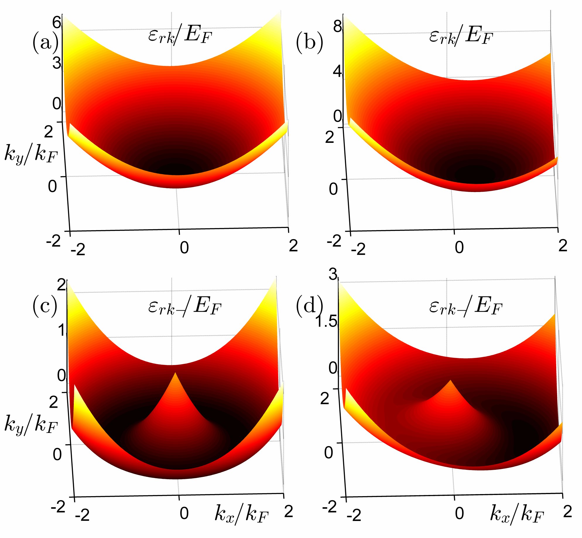
Figure 1: (Color online) Local dispersion relations for (a) $\Omega=0$ and $\alpha=0$: the usual paraboloid, (b) $\Omega\neq 0$ and $\alpha=0$: finite momentum states that are energetically favored by rotation result in a shifted paraboloid, (c) $\Omega=0$ and $\alpha\neq 0$: the negative-helicity band has a degenerate circular minima, and (d) $\Omega\neq 0$ and $\alpha\neq 0$: rotation causes an asymmetric minimum.

III.1 Trapped Fermi gas
($\omega\neq 0$, $\alpha=0$ and $\Omega=0$)

The first analytically-tractable limit is a usual 2D Fermi gas with neither Rashba coupling nor rotation, for which case the local dispersion relation is simply a paraboloid with its minimum at the origin $\mathbf{k}=\mathbf{0}$. This is shown in Fig. 1(a) for completeness, and the Fermi surface is trivially a circle around the origin. Since the DOS of a uniform Fermi gas is a constant in 2D, the LDOS of a trapped gas can be written within the LDA approach as $D_{r}(\epsilon)=MA\Theta(\epsilon_{r})/\pi,$ where $\Theta(x)$ is the Heaviside-step function and $\epsilon_{r}=\epsilon-V_{r}$, and it is shown in Fig. 2(a). The resulting number density is an inverted parabola, $n_{r}=M(E_{F}-M\omega^{2}r^{2}/2)/\pi,$ where $E_{F}$ is the Fermi energy at the trap center, and the Thomas-Fermi radius $R_{F}$ is given by definition $n_{R_{F}}=0$ as $R_{F}=\sqrt{2E_{F}/(M\omega^{2})}.$ In addition, the central density can be written as $n_{0}=k_{F}^{2}/(2\pi)$, where $k_{F}$ is the Fermi momentum in such a way that $E_{F}=k_{F}^{2}/(2M)=\omega\sqrt{N}.$ We use $E_{F}$, $k_{F}$ and $R_{F}$ as, respectively, the energy, momentum and length scales in our numerical calculations.

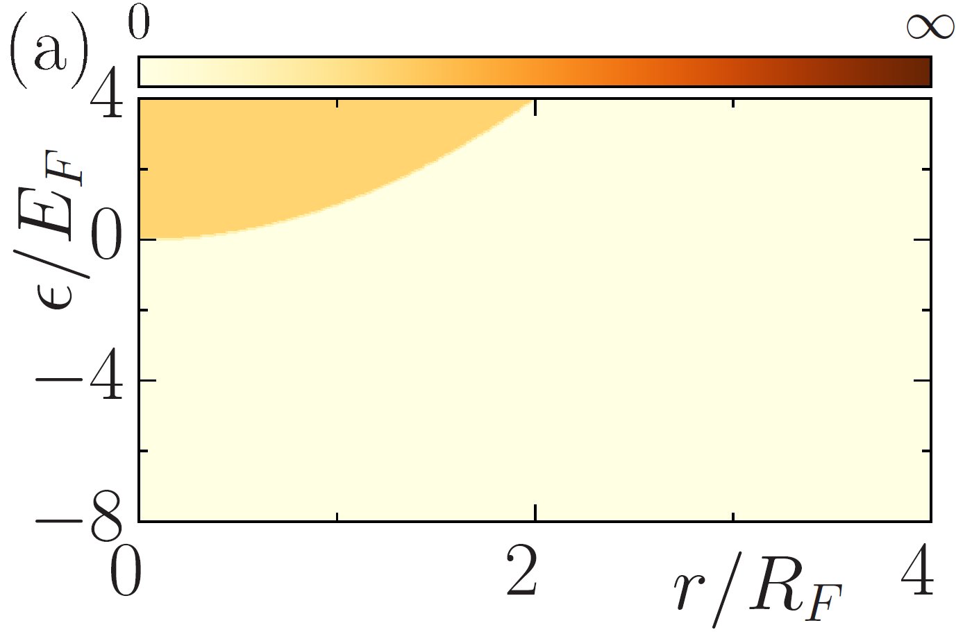
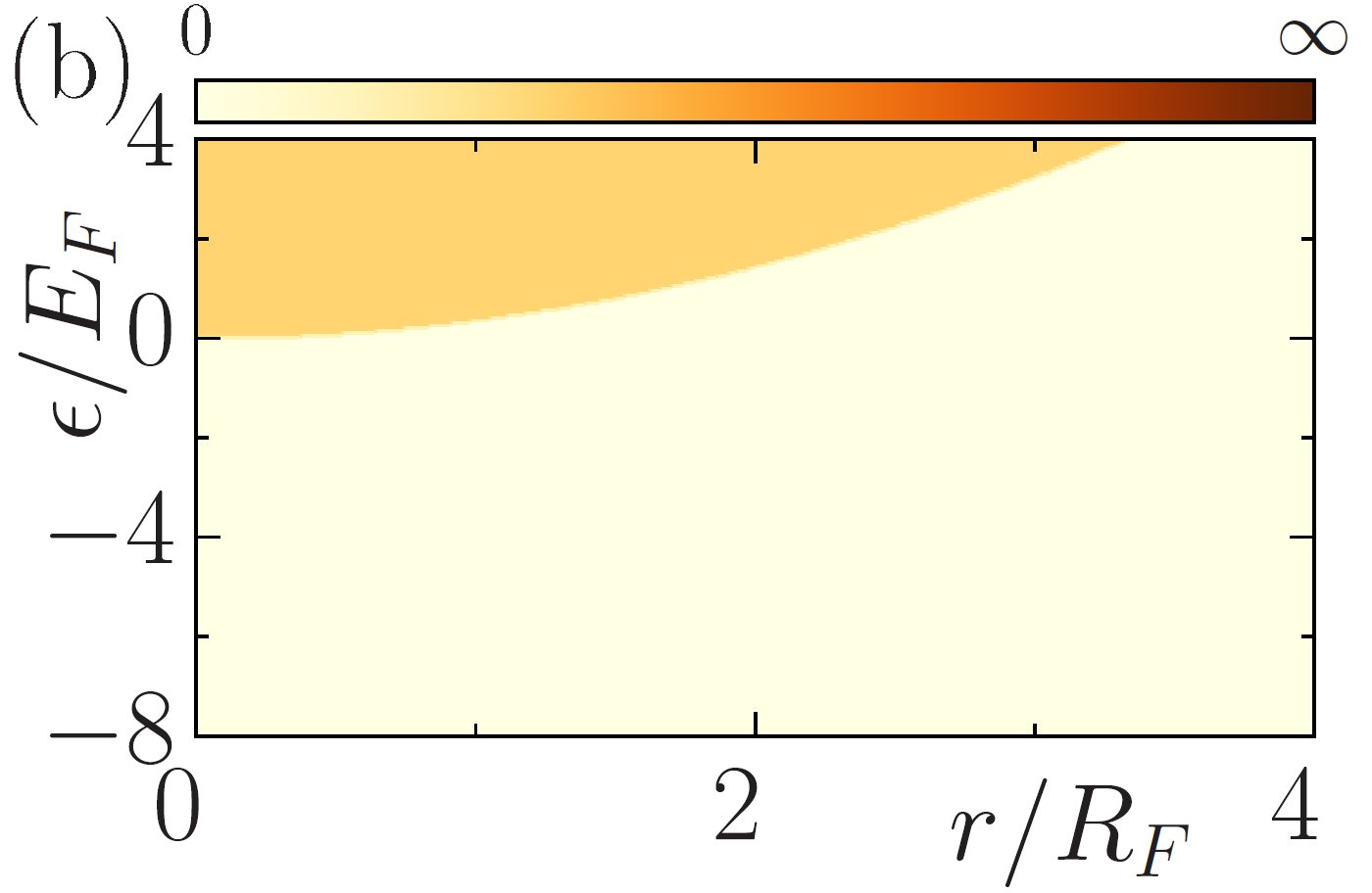
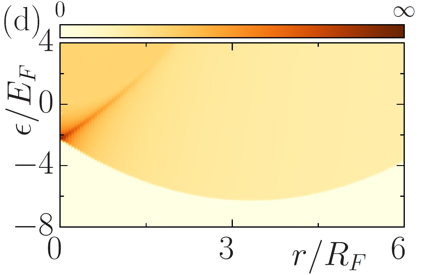
Figure 2: (Color online) Local energy density of states (LDOS) in the trap within the LDA approach. In the absence of a Rashba coupling, the LDOS is a constant except for the outward extension due to rotation as shown in (a) for $\Omega=0$ and $\alpha=0$ and (b) for $\Omega=0.4\omega$ and $\alpha=0$. In the absence of rotation, Rashba coupling enhances the LDOS for the lowest energies as shown in (c) for $\Omega=0$ and $\alpha=3E_{F}/k_{F}$. In the generic case shown in (d) for $\Omega=0.8\omega$ and $\alpha=3E_{F}/k_{F}$, rotation not only pushes the minimum of the LDOS away from the trap center but it also removes the divergence for $r\neq 0$ as discussed in the main text.

III.2 Trapped Fermi gas with Rashba coupling
($\omega\neq 0$, $\alpha\neq 0$ and $\Omega=0$)

The second analytically-tractable limit is a 2D Fermi gas with Rashba coupling, for which case the main effect of this coupling on the trap profiles is to increase the number density at the trap center through the increased low-energy LDOS. To see this effect, we first note that, by breaking the spin-rotation symmetry, the Rashba coupling splits the local dispersion relation into two ($s=\pm$) local helicity branches. Here, the spin is oriented parallel to the momentum $\mathbf{k}$ in the higher-energy $+$ branch and anti-parallel in the lower-energy $-$ one. While the energy of the $+$ branch increases monotonically with $k$, the minimum of the spectrum is shifted to finite momentum for the $-$ branch forming a circle with radius $k=M\alpha$ as shown in Fig. 1(c). Thus, in the local regions with $\mu_{r}>0$, there are two circular Fermi surfaces around the origin in $\mathbf{k}$ space corresponding to $+$ and $-$ branches. When the $+$ branch disappears for $\mu_{r}\leq 0$, an additional circular Fermi surface appears in the $-$ branch, in which case, however, all of the $\mathbf{k}$ states that are below the Fermi energy have finite momentum.

Then, within the LDA approach, it is easy to show that the LDOS are given by $D_{rs}(\epsilon)=MA(1-sM\alpha/\sqrt{M^{2}\alpha^{2}+2M\epsilon_{r}})/(2\pi)$ in the local regions with $\epsilon_{r}>0$, and $D_{rs}(\epsilon)=(1-s)M^{2}A\alpha\Theta(M^{2}\alpha^{2}+2M\epsilon_{r})/(2\pi\sqrt{M^{2}\alpha^{2}+2M\epsilon_{r}})$ in the local regions with $\epsilon_{r}\leq 0$. This indicates that, in sharp contrast to the $\epsilon_{r}>0$ regions where the total LDOS is clearly unaffected by the Rashba coupling, it displays a 1D-like energy dependence in the $\epsilon_{r}\leq 0$ regions arising solely from the $-$ branch, i.e., the divergence of LDOS in the local regions satisfying the condition $\epsilon_{r}=-M\alpha^{2}/2$ is very much like that of a uniform Fermi gas in 1D. This behavior is a reflection of the degenerate minima discussed above, and it gives rise to the enhanced low-energy LDOS shown in Fig. 2 (c). This effect reduces the radius of the gas as the number density increases around the trap center due to the increased low-energy LDOS.

Furthermore, since the Rashba coupling indirectly affects the density profile through the depletion of particles from the $+$ branch, we determine the critical radius $r_{c}=[-2\alpha^{2}/\omega^{2}+\sqrt{4\alpha^{4}/(3\omega^{4})+R_{F}^{4}}]^{1/2}$ for the complete depletion by setting $\mu_{r_{c}}=0$. In addition, we find $n_{rs}=M^{2}(-s\alpha+\sqrt{\alpha^{2}+2\mu_{r}/M})^{2}/(4\pi)$ in the local regions with $\mu_{r}>0$ or equivalently $r<r_{c}$, and $n_{r+}=0$ and $n_{r-}=M^{2}\alpha\sqrt{\alpha^{2}+2\mu_{r}/M}/\pi$ in the local regions with $\mu_{r}<0$ or equivalently $r>r_{c}$. Since $r_{c}>0$ for weak couplings, there is an outer ring-shaped region in the trap where the local $+$ branch is completely empty. Setting $r_{c}=0$, we find the critical Rashba coupling $\alpha_{c}=\sqrt[4]{6}E_{F}/k_{F}$, beyond which the $+$ branch is never occupied in the entire trap. We note that even though the number density acquires a relatively simple form when $\alpha>\alpha_{c}$, it is quite different from the usual inverted-parabola dependence of a trapped Fermi gas discussed in Sec. III.1. Furthermore, the edge of the gas can be extracted from the number density as $R_{O}^{0}=[-\alpha^{2}/\omega^{2}+\sqrt{4\alpha^{4}/(3\omega^{4})+R_{F}^{4}}]^{1/2}$ for $\alpha<\alpha_{c}$, and $R_{O}^{0}=R_{F}[3E_{F}/(4\alpha k_{F})]^{1/3}$ for $\alpha\geq\alpha_{c}$, showing explicitly that the edge of the gas $R_{O}^{0}$ moves inward with increasing $\alpha$ and the gas contracts. By integrating the number density, we also find $\mu=-\alpha^{2}M+\sqrt{\alpha^{4}M^{2}/3+E_{F}^{2}}$ for $\alpha<\alpha_{c}$, and $\mu=-\alpha^{2}M/2+[6E_{F}^{2}/(\alpha\sqrt{2M})]^{2/3}/4$ for $\alpha>\alpha_{c}$.

III.3 Trapped Fermi gas with adiabatic rotation
($\omega\neq 0$, $\alpha=0$ and $\Omega\neq 0$)

Another analytically-tractable limit is a 2D Fermi gas with adiabatic rotation, for which case the main effect of rotation on the trap profiles is to spread out the number density supported by the imparted centripetal acceleration on the particles. To see this effect, we first note that, by breaking the inversion symmetry of the dispersion relation, i.e., tilting of the excitation spectrum, rotation causes an asymmetry in $\mathbf{k}$ space. This shifts the minimum of the paraboloid from the origin shown in Fig. 1(a) to a finite $k=r\Omega M$ as shown in Fig. 1(b) where the Fermi surface is a circle centered around this finite momentum.

We find that the LDOS is simply given by $D_{r}(\epsilon)=MA\Theta(\epsilon_{r}+M\Omega^{2}r^{2}/2)/\pi,$ showing that it remains to be a constant except for the radial extention, and that its parabolic shape is retained as shown in Fig. 2(b). As a consequence, $\mu=E_{F}\sqrt{1-\Omega^{2}/\omega^{2}},$ and the resultant number density is still an inverted parabola $n_{r}=M^{2}[2\mu/M-(\omega^{2}-\Omega^{2})r^{2}]/(2\pi).$ We note that since the curvature of the trap profile decreases with increasing $\Omega$, the edge of the gas $R_{O}^{0}=R_{F}(1-\Omega^{2}/\omega^{2})^{-1/4}$ expands with $\Omega$ until $\Omega=\omega$, beyond which the trap cannot supply the necessary centripetal acceleration. In addition, the associated mass-current density $J^{\theta}_{r}=Mn_{r}\Omega r$ is exactly of the form of a rigidly-rotating gas. We note in passing that the asymmetric occupation of the finite-angular-momentum states with respect to the rotation along with and opposite to the azimuthal direction causes a pair-breaking effect on the Cooper pairs with zero center-of-mass momentum, as further discussed in Sec. IV.3.

Figure 3: The critical rotation frequency $\Omega_{c}^{0}$ for the depletion of the non-interacting number density at the trap center at $T=0$. Increasing the Rashba coupling beyond a critical value transforms the disk-shaped density of the Fermi gas into a ring-shaped annulus. While an annulus may ultimately form for any $\Omega<\omega$ as long as $\alpha$ is sufficiently high, $\Omega_{c}^{0}\to\omega$ in the $\alpha\to 0$ limit signifying the crucial interplay between Rashba coupling and adiabatic rotation for this effect.

III.4 Trapped Fermi gas with Rashba coupling and rotation
($\omega\neq 0$, $\alpha\neq 0$ and $\Omega\neq 0$)

Having shown analytically that the Rashba coupling and adiabatic rotation have competing effects on the trap profiles, we are ready to discuss the generic case with arbitrary $\Omega$ and $\alpha$, for which case the main effect of their interplay is to change the number density from the shape of a disk to a ring-shaped annulus. To see this effect, we first note that, by breaking the degeneracy in the lowest-energy states, rotation tilts the minima of the $-$ branch as shown in Fig. 1(d). Since the tilting-effect is proportional to $k$, it is further enhanced by the Rashba coupling, giving rise to three topologically-distinct Fermi surfaces for the $-$ branch and one for the $+$ one. For instance, in the local regions with $\mu_{r}>0$, the local Fermi surface of the $-$ branch is a circle around some finite $k$. In the local regions with $\mu_{r}<0$, however, while the local Fermi surface is a deformed ring centered around the origin when $\sqrt{-2\mu_{r}/M}-\alpha\leq-2\Omega r,$ it is of the crescent shape when $|\sqrt{-2\mu_{r}/M}-\alpha|\leq\Omega r.$ In contrast, the local Fermi surface of the $+$ branch is a deformed circle centered at some finite $k$. Note that, unlike the non-rotating case discussed in Sec. III.2, the $+$ branch is locally occupied even in the regions with $\mu_{r}\leq 0$ as long as $\sqrt{-4\mu_{r}}+\alpha\leq 2\Omega r$.

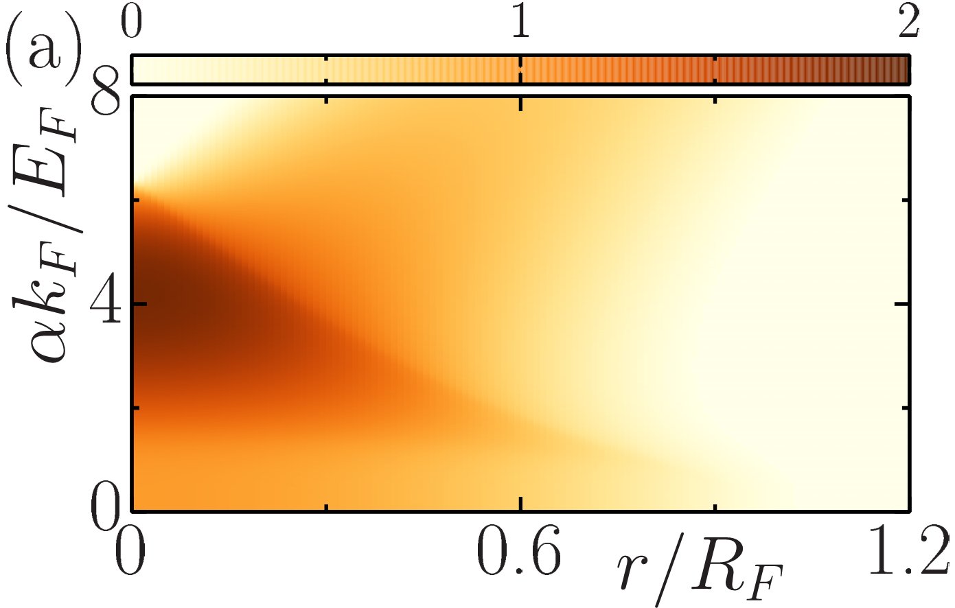
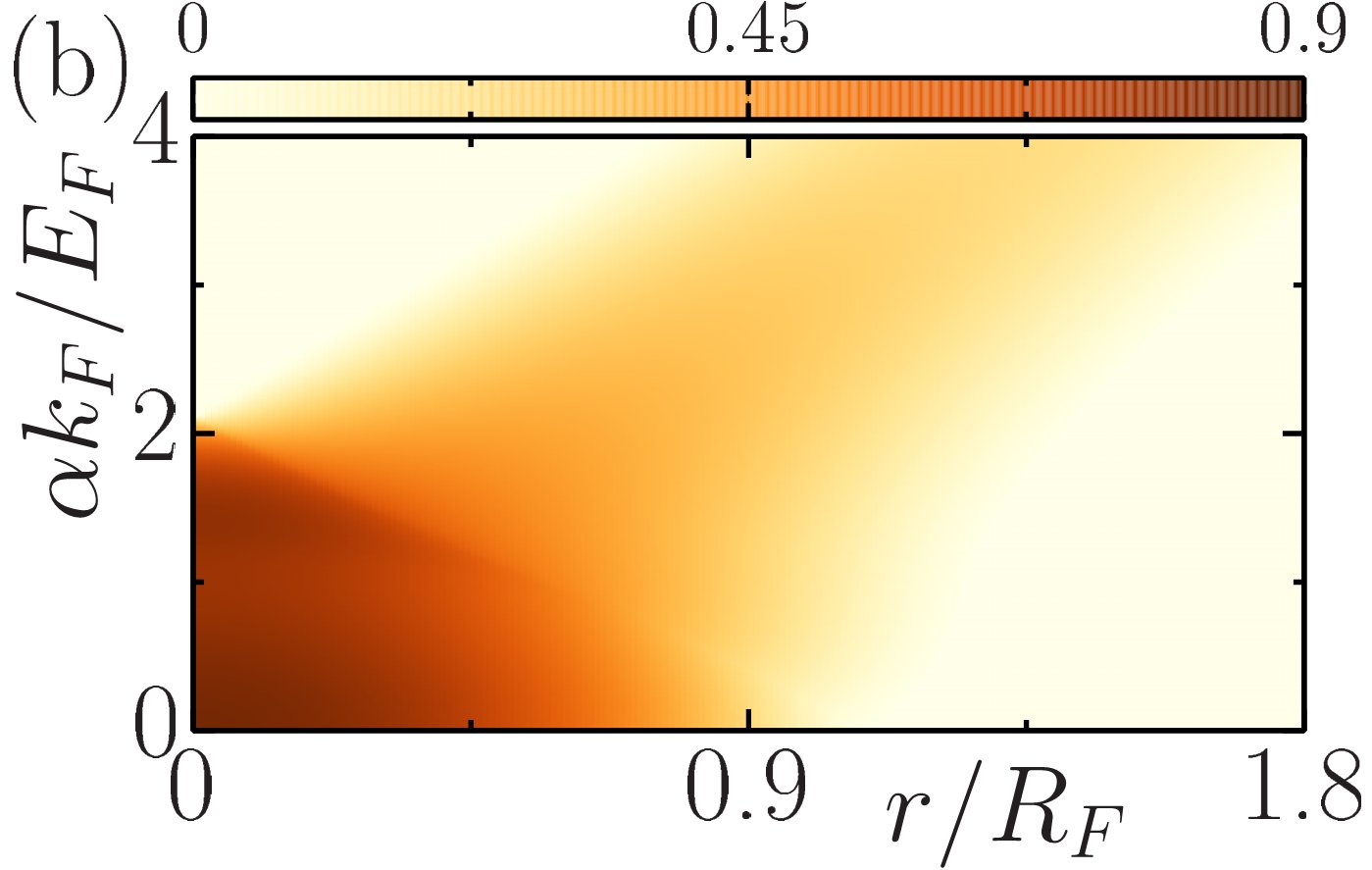
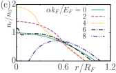
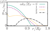
Figure 4: (Color online) Non-interacting number-density maps at $T=0$ with changing Rashba coupling for (a) $\Omega=0.15\omega$ and (b) $\Omega=0.5\omega$. A few exemplary radial density profiles are plotted in (c) and (d), showing explicitly that the rotating Fermi gas eventually takes on a ring-shaped annulus with increasing $\alpha$.

The radial position of the lowest-energy state in the trap can be determined by minimizing $\varepsilon_{r\mathbf{k}-}$ with respect to both $\mathbf{k}$ and $r$, leading to $k=\alpha M\omega^{2}/(\omega^{2}-\Omega^{2})$ with $\theta_{\mathbf{k}}=\pi/2$, i.e., opposite to the direction of the mass-current density, and $r=\alpha\Omega/(\omega^{2}-\Omega^{2}).$ Note that $k\to 0$ and $r\to 0$ is recovered for the usual case when $\alpha\to 0$ and $\Omega\to 0$. To gain further insight, we calculate the LDOS via the following representation of the Dirac-delta function $\delta(x)\approx(1/\pi)\lim_{\varsigma\to 0}\varsigma/(x^{2}+\varsigma^{2})$ with $\varsigma=10^{-3}$, and the results are shown in Fig. 2(d). We see that, by breaking the degeneracy of the lowest-energy states in the $-$ branch, rotation removes the 1D-like divergence from the LDOS profile for all $r\neq 0$. Recall that $r=0$ is immune to the direct-effects of rotation. In addition, since the higher the angular momentum of the single-particle state the further away its localization distance from the trap center, we conclude that the lowest-energy states have finite angular momentum, and that a comparison between Figs. 2(c) and 2(d) reveals that the lowest-energy of the finite-angular-momentum states is lower than the lowest-energy of the non-rotating gas. Thus, depending on the strengths of Rashba coupling and adiabatic rotation, it may be energetically more costly for any of the particles to occupy the trap center, in which case the number density forms a ring-shaped annulus.

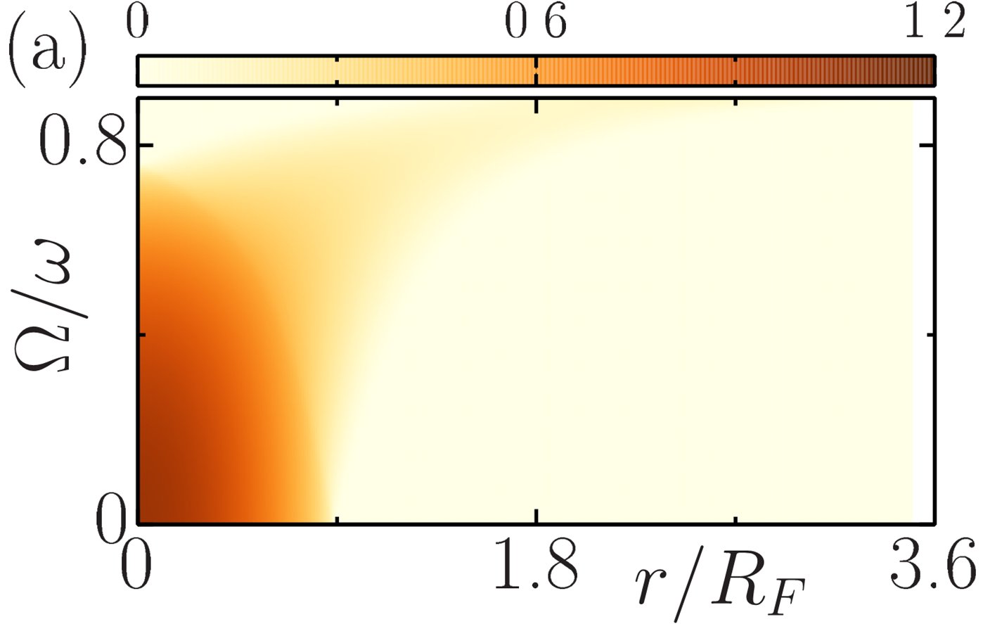
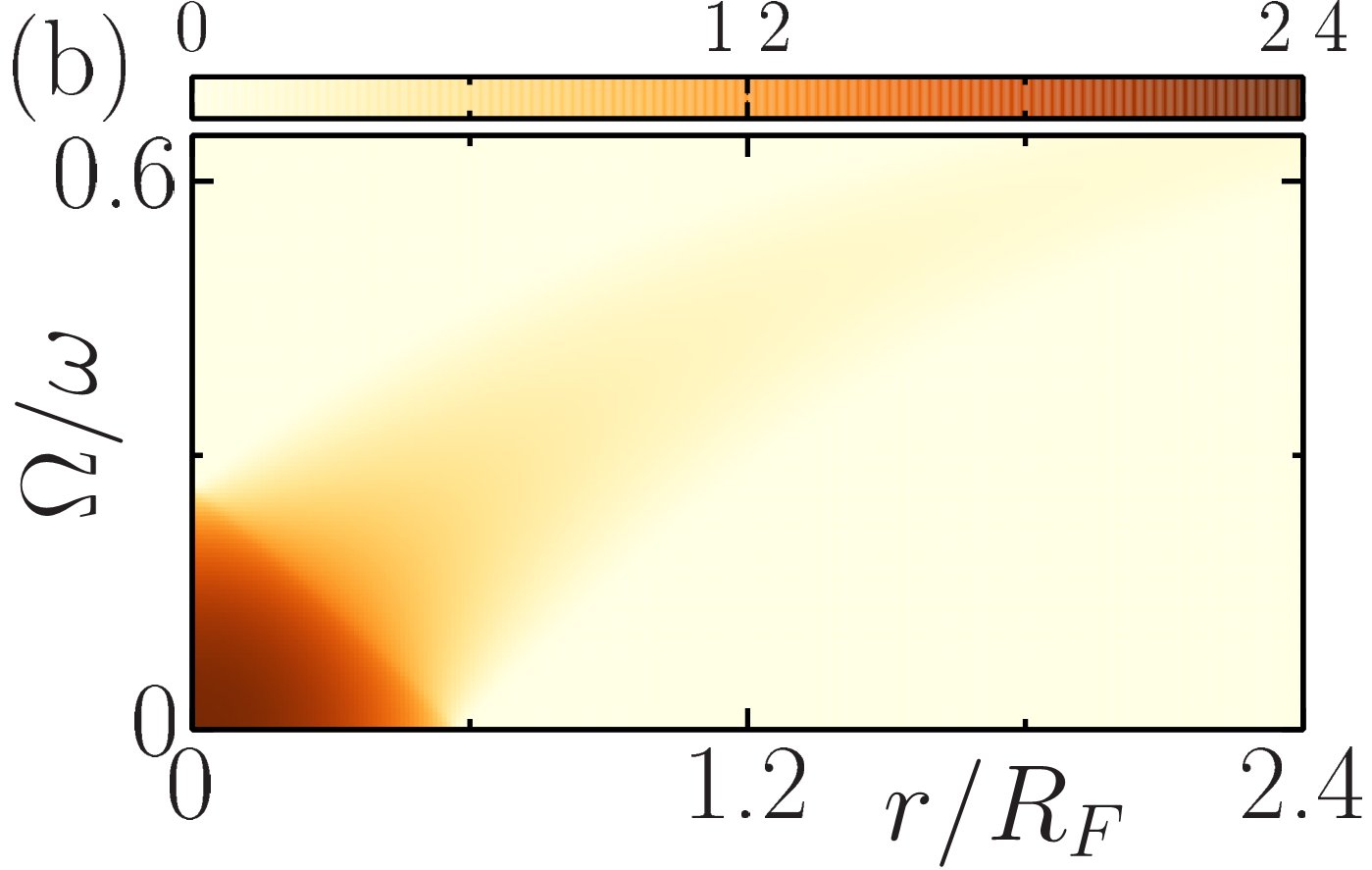
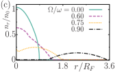
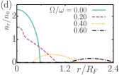
Figure 5: (Color online) Non-interacting number-density maps at $T=0$ with changing rotation frequency for (a) $\alpha=1k_{F}/E_{F}$ and (b) $\alpha=4k_{F}/E_{F}$. A few exemplary radial density profiles are plotted in (c) and (d), showing explicitly that the Rashba-coupled Fermi gas eventually takes on a ring-shaped annulus with increasing $\Omega$.

Alternatively, the depletion of the number density at the trap center and the accompanying formation of a ring-shaped annulus can also be deduced analytically as follows. First of all, the central density turns out to be $n_{r=0}=M(\alpha^{2}M+\mu)/\pi$ for $\mu\geq 0$, and $n_{r=0}=\alpha M^{2}\sqrt{\alpha^{2}+2\mu/M}/\pi$ for $\mu<0$, showing explicitly that $n_{r=0}=0$ when the parameters satisfy the critical condition $\alpha^{2}+2\mu/M\leq 0$. Here, $\Omega$ enters into this condition implicitly through its dependence on $\mu$. Then, we note that the locations at which the number density vanishes, i.e., the local Fermi surface disappears, are exactly the inner and outer radii forming the edges of the gas. Since the presence of a local Fermi surface implies real solutions for $k^{s}_{1,2}$, we find the edges by setting the square root to zero in Eq. (15), i.e., $M(\Omega r-s\alpha)^{2}+2\mu_{r}=0$, leading to

$$R_{I,O}^{0}=R_{F}\frac{\omega\Omega\alpha\pm\omega\sqrt{\alpha^{2}\omega^{2}+2\mu(\omega^{2}-\Omega^{2})/M}}{k_{F}(\omega^{2}-\Omega^{2})/M},$$ (16)

where $I$ ($O$) denotes the inner (outer) edge. The gas may form an annulus only if the inner radius satisfies $R_{I}^{0}\geq 0$, leading again to the critical condition $\alpha^{2}+2\mu/M\leq 0$. Thus, the critical rotation frequency $\Omega_{c}^{0}$ for the emergence of such an annulus can be calculated by a self-consistent solution of the number equation together with the critical condition $\alpha^{2}+2\mu/M=0$. The resultant phase diagram is shown in Fig. 3, where $\Omega_{c}^{0}$ decreases monotonically with increasing $\alpha$, and it is in perfect agreement with our fully-numerical solutions for the trap profiles as illustrated below. We also note in passing that while the gas never forms an annulus in the $\alpha\to 0$ limit given the upper bound on $\Omega$ as the harmonic potential can only trap the particles for $\Omega<\omega$, it may form an annulus at any finite $\alpha$ with $\Omega_{c}^{0}<\omega$.

In Figs. 4 and 5, the trap profiles are shown for a wide range of parameters. For instance, we set $\Omega=0.15\omega$ in Figs. 4(a) and 4(c), and plot the number-density maps in the entire trap as a function of $\alpha$ together with a few exemplary radial density profiles. As discussed above, the Rashba coupling not only increases the LDOS around the trap center but it also favors energetically some finite-angular-momentum states, causing simultaneously an increase in the central density due to the former effect and an expansion of the edge due to the latter one as a function of $\alpha$. This competition sharply decreases the number density away from the trap center. Once $\alpha$ approaches to the critical value $\alpha=\sqrt{-2\mu/M}$, the latter effect gradually dominates leading to a reduction in the central density as the gas continues to expand. There is an intriguing appearance of an additional local maximum in the number density in the vicinity of critical $\alpha$, beyond which it is completely depleted at the trap center, and the radius $R_{I}^{0}$ of the depleted region grows linearly with $\alpha$. We consider a higher $\Omega=0.5\omega$ in Figs. 4(b) and 4(d), showing that the central density decreases and the edge expands immediately with increasing $\alpha$, leading to the depletion of the trap center at a much lower critical $\alpha$. Similarly, these effects are also seen in Fig. 5, where $\Omega$ is increased at fixed $\alpha$ values. In contrast to Fig. 4, here we see that a faster rotation leads to a monotonic reduction of the central density and a monotonic expansion of the edge.

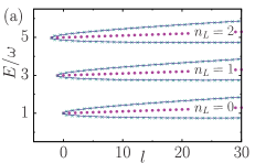
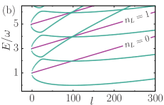
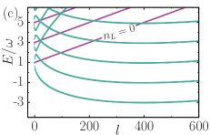
Figure 6: (Color online) Energy levels as a function of angular momentum for a rapidly-rotating Fermi gas with Rashba coupling in the Landau regime when $\Omega=0.99\omega$. Here, $\alpha=0$ limit is shown in purple dots for the first three Landau levels as a reference. (a) $\alpha=0.2\sqrt{\omega/M}$: Rashba coupling splits each of the Landau levels into two helicity branches with a widening energy gap in between as a function of angular momentum. (Blue solid line corresponds to the perturbation expression given in the text.) (b) $\alpha=0.4\sqrt{\omega/M}$: the helicity branches display avoided level crossings. (c) $\alpha=0.8\sqrt{\omega/M}$: all of the negative-helicity branches not only occupy lowest energies but they also develop minimum at finite angular momentum.

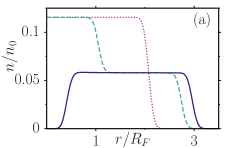
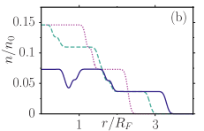
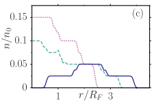
Figure 7: (Color online) Radial density profiles at $T=0$ in the Landau regime when $\Omega=0.99\omega$. The purple-dotted, green-dashed and blue-solid lines correspond, respectively, to higher Rashba couplings (in units of $\sqrt{\omega/M}$) where $\alpha=\{0,0.2,0.4\}$ in (a) with $N=750$ particles in the lowest-Landau level, $\alpha=\{0,0.2,0.4\}$ in (b) with $N=900$ particles in the first two Landau levels, and $\alpha=\{0,0.4,0.8\}$ in (c) with $N=1600$ particles in the first three Landau levels. These intriguing profiles directly reflect the corresponding energy-level structures shown in Fig. 6, where the higher the angular momentum of the single-particle state the further away its localization distance from the trap center.

III.5 Rapidly-rotating Fermi gas with Rashba coupling
($\omega\neq 0$, $\alpha\neq 0$ and $\Omega\to\omega$)

Since the effects of rotation are analogous to those of an effective magnetic field on a particle, where the Coriolis force on a neutral atom mimics the Lorentz force on a charged particle, a rapidly-rotating Fermi gas may form highly-degenerate Landau levels in the $\Omega\to\omega$ limit and exhibit an integer quantum-Hall effect Ho2000 . Since the LDA approach fails to capture the correct physics in the Landau regime of a rapidly-rotating Fermi gas, we resort to exact quantum-mechanical calculations in the following discussion.

In the absence of a Rashba coupling, and assuming $\omega_{-}=\omega-\Omega$ is small, it is convenient to label the single-particle states with $n_{L}=(n-l)/2$ the Landau-level index and $l$ the angular momentum, leading to the dispersion relation $\varepsilon_{n_{L}l}=\omega(2n_{L}+1)+\omega_{-}l.$ Here, $n_{L}=\{0,1,2,\cdots\}$ and $l=\{0,1,2,\cdots\}$, so that $\varepsilon_{n_{L}l}$ increases linearly with $l$. Note that all of the consecutive Landau levels are separated by an equal gap $2\omega$ for any given $l$, and that each of these energy states are two-fold degenerate due to the pseudo-spin $\sigma$ of the particles. We set $\Omega=0.99\omega$ in Fig. 6, and show this spectrum in purple for the first three Landau levels as a reference. Since each fully-filled Landau level below a given $\mu$ results in a uniform density, this spectrum gives rise to a ziggurat-shaped density profile in the trap, where the number of plateaus directly reflects the number of underlying Landau levels involved. For instance, such staircase-looking number densities are clearly visible in Figs. 7(a), 7(b) and 7(c), where $\alpha=0$ limits are shown as the purple-dotted lines corresponding, respectively, to one, two and three fullly-filled Landau levels.

When $\alpha\neq 0$, by breaking the spin-rotation symmetry, the Rashba coupling lifts the spin degeneracy, leading to two ($s=\pm$) helicity branches for each Landau level. For instance, in the perturbative regime when $\alpha\ll 2a_{0}\omega$ with $a_{0}=1/\sqrt{M\omega}$ the characteristic harmonic-oscillator length scale, we approximately find $\varepsilon_{n_{L},l,s}=\omega(2n_{L}+1)+\omega_{-}l+\omega_{-}/[2+2s\sqrt{1+\alpha^{2}(n_{L}+l+1)/(a_{0}\omega_{-})^{2}}].$ We checked that this expression is in excellent agreement with all of the exact results presented in Fig. 6, e.g., our perturbative results (solid blue lines) are shown to lie right on top of the exact ones (green crosses) in Fig. 6(a). As $l$ gets higher, Fig. 6(b) shows that the helicity branches ultimately display avoided level crossings. In addition, as $\alpha$ is increased to $\alpha\gtrsim a_{0}\omega_{-}$, all of the negative-helicity branches develop a minimum near some finite $l$ given by $l_{\textrm{min}}=\alpha^{2}/(4a_{0}\omega_{-})^{2}.$ This is shown in Fig. 6(c) for $\alpha=0.8\sqrt{\omega/M}$, where all of the energy gaps between the two consecutive same-helicity branches are approximately $2\omega$ in this perturbative regime. Thus, the main effect of weak Rashba coupling on the trap profiles is expected to be doubling of the number of plateaus in the number density as a reflection of the lifted spin degeneracy of the Landau levels. In addition, the interplay of Rashba coupling and rapid rotation may ultimately lead to the formation of a ring-shaped annulus with a ziggurat texture as shown in Fig. 7(c).

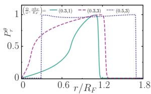
Figure 8: (Color online) The azimuthal component of the average spin-polarization increases monotonically from zero at the trap center to unity at the edge, and the gas is almost fully polarized within the ring-shaped annulus.

III.6 Spin-polarization textures

Since the Rashba coupling splits the spin degeneracy of the free-particle energy bands into $\pm$-helicity branches with spins oriented parallel/anti-parallel to the momentum $\mathbf{k}$, and the rotation favors momentum states that are parallel to the direction of mass-current density, their interplay polarizes the average spin of the particles in the azimuthal direction. The azimuthal component of the local average spin-polarization texture can be written as $P_{\mathbf{r}}^{\theta}=-P_{\mathbf{r}}^{x}\sin\theta_{\mathbf{r}}+P_{\mathbf{r}}^{y}\cos\theta_{\mathbf{r}},$ with its components defined in Sec. II.2.2. In the absence of a Zeeman field as considered in this paper, we note that the average spin of the system is unpolarized not only in the $\alpha\to 0$ as the spin and $\mathbf{k}$ are uncoupled, but also in the $\Omega\to 0$ limit as the contributions of $\pm\mathbf{k}$ states are equal in magnitude but opposite in direction. Therefore, the interplay between Rashba coupling and adiabatic rotation is proved to be crucial for the appearance of spin textures.

For instance, the radial spin-polarization profiles are shown in Fig. 8 for three sets of $\alpha$ and $\Omega$. The azimuthal polarization increases from zero at the trap center as $r=0$ is immune to the direct-effects of rotation, and reaches unity at the edge as only the non-degenerate lowest-energy states of the negative-helicity branch having anti-parallel spin orientations with respect to the angular direction are occupied. As a result of the disappearance of the positive-helicity band and increasing asymmetry in the energy dispersion, we find that increasing $\alpha$ and $\Omega$ gradually increases the polarization in the intermediate region between the trap center and the edge as well. Furthermore, we also find that the polarization approaches to unity everywhere in the trap once the number density forms a ring-shaped annulus, and this is shown in Fig. 8 when $\Omega=0.5\omega$ and $\alpha=3E_{F}/k_{F}$.

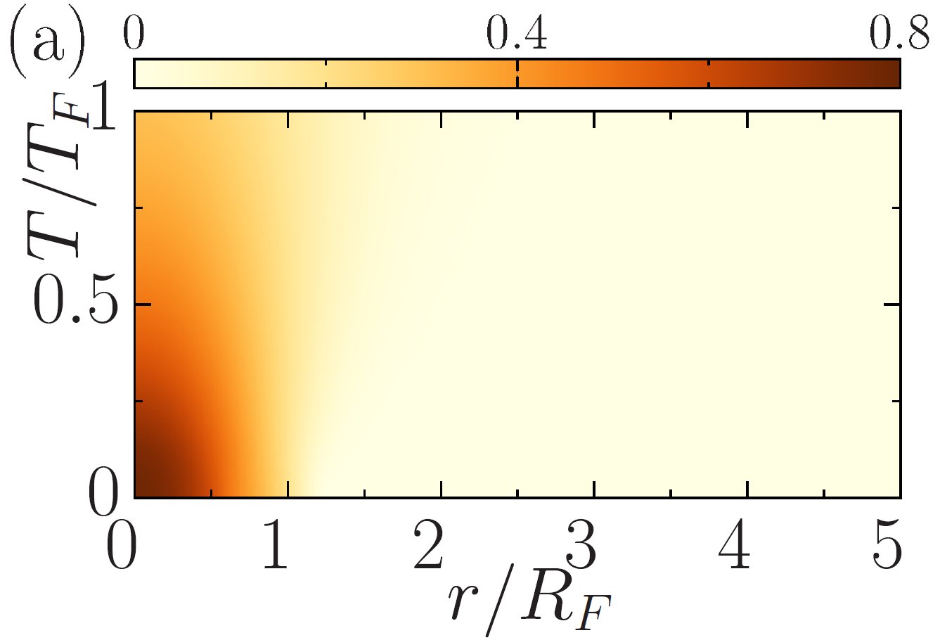
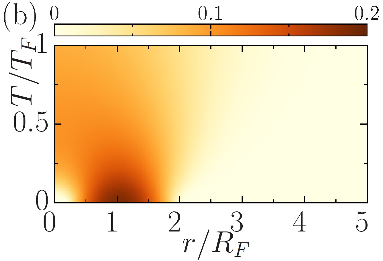
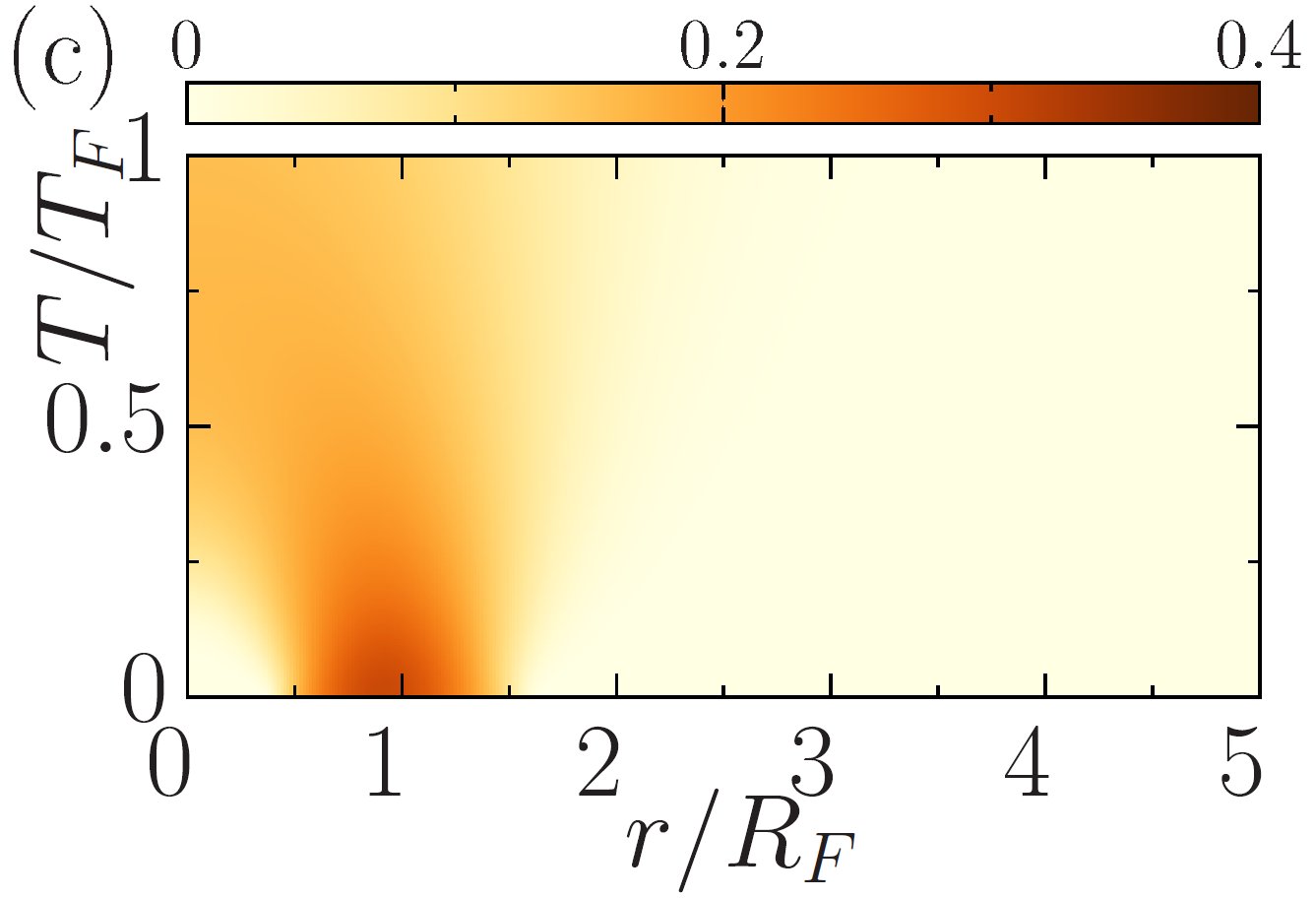
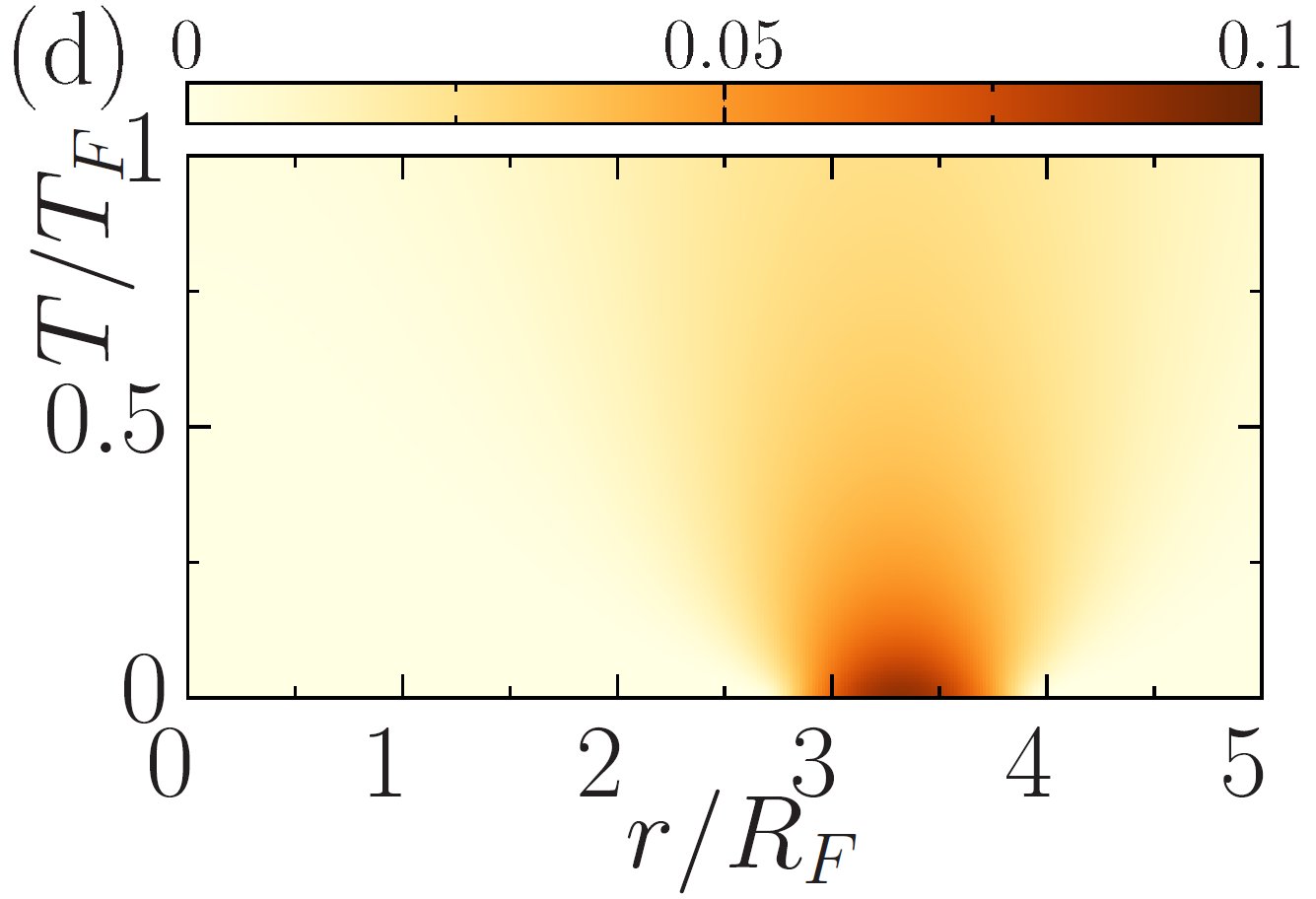
Figure 9: (Color online) Non-interacting number-density maps at finite $T$. Increasing either $\Omega$ or $\alpha$ from (a) $\Omega=0.5\omega$ and $\alpha=1E_{F}/k_{F}$, the disk-shaped profile transform into a ring-shaped annulus for (b) $\Omega=0.8\omega$ and $\alpha=1E_{F}/k_{F}$ and (c) $\Omega=0.5\omega$ and $\alpha=3E_{F}/k_{F}$. While the depletion of the central density that is clearly visible at low $T$ is eventually blurred by the thermal broadening, it can be sustained at very high $T$ with increasing either $\Omega$ and/or $\alpha$. This is shown in (d) for $\Omega=0.8\omega$ and $\alpha=3E_{F}/k_{F}$.

III.7 Thermal effects

Before moving to the effects of interactions, here we conclude the non-interacting Fermi gas section by addressing how much of our zero-temperature trap profiles survives at finite $T$. For this purpose, we fix $\Omega$ and $\alpha$ in Fig. 9, and plot the number-density maps in the entire trap as a function of $T$. It is clearly shown that the thermal-broadening effects on the number density are most significant in the ring-shaped regions, as the system eventually recovers the disk-shaped profile at sufficiently high $T$. However, it is encouraging to see that, by increasing either $\Omega$ and/or $\alpha$, a visible ring-shaped annulus may still form at very high $T$ that is of the order of a Fermi temperature $T_{F}=E_{F}/k_{B}$, making its experimental observation quite feasible. We note that the number density first appears as nearly flat in a wide region, the width of which is of the order of $R_{F}$, at some intermediate $T$, and then it ultimately attains the usual Gaussian shape at high $T$.

Having convincingly shown that the interplay between the effects of Rashba coupling on the LDOS and the Coriolis effects caused by rotation gives the number density of a non-interacting Fermi gas a characteristic ring-shaped annulus form that survives at experimentally-accessible temperatures, we next analyze how this interplay effects the trap profiles of an interacting Fermi gas, and the associated SF properties.

IV Interacting Fermi gas

Armed with a thorough understanding of the generic properties of a non-interacting Fermi gas with Rashba coupling under adiabatic rotation, we are ready to discuss the effects of interaction as characterized by the two-body binding energy $E_{b}>0$ in vacuum. The SF ground state of an interacting Fermi gas is protected by an energy gap in the low-energy excitation spectrum, and the gap is directly related to the order parameter $\Delta_{\mathbf{r}}$ of the underlying Cooper pairs that are made of time-reversed particles. Thus, while this order parameter acts as an energy barrier and protects the pairs, by breaking the time-reversal symmetry, rotating a SF Fermi gas may energetically favor a state with broken pairs beyond a critical rotation frequency. Our primary objective here is to study such a pair-breaking mechanism that is induced by the Coriolis effects on superfluidity, where we calculate the critical rotation frequencies both for the onset of pair breaking and for the complete destruction of superfluidity in the system. In particular, by comparing the results of fully-quantum-mechanical BdG approach with those of semi-classical LDA one, we construct extensive phase diagrams consisting of non-rotating gapped SF, partially-rotating gSF and rigidly-rotating N regions. These diagrams allow us to predict all sorts of phase profiles in the trap for a wide-range of parameter regimes, where the interplay between Rashba coupling and adiabatic rotation may favor, e.g., an outer N edge that is completely phase separated from the central SF core by vacuum.

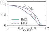
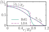
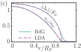
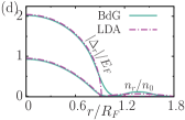
Figure 10: (Color online) The radial order-parameter and number-density profiles at $T=0$ showing an excellent agreement between the LDA and BdG results, where (a) $E_{b}=0.5E_{F}$, $\alpha=0$ and $\Omega=0$, (b) $E_{b}=0.5E_{F}$, $\alpha=0$ and $\Omega=0.7\omega$, (c) $E_{b}=0.5E_{F}$, $\alpha=2E_{F}/k_{F}$ and $\Omega=0$ with $N=500$ particles, and (d) $E_{b}=2E_{F}$, $\alpha=2E_{F}/k_{F}$ and $\Omega=0.7\omega$ with $N=100$ particles.

Similar to Sec. III, we again rely mostly on the LDA approach throughout this section, given that the LDA results are in very good agreement with those of BdG ones for a wide-range of parameter regimes and with the additional advantage that they permit analytical insights into the limiting cases. For instance, we benchmark our LDA and BdG results in Fig. 10, where we set $N=500$ particles with $E_{b}=0.5E_{F}$ and $E_{c}\sim 27E_{F}$ in Fig. 10(a), 10(b) and 10(c), and $N=100$ particles with $E_{b}=2E_{F}$ and $E_{c}\sim 60E_{F}$ in Fig. 10(d). It is not surprising that the LDA approach works really well in the regions where the changes in $|\Delta_{\mathbf{r}}|$ and $n_{r}$ are slow. To gain as much insight as possible into the basic properties of an interacting Fermi gas, we again discuss these quantities first in a few analytically-tractable limits, prior to the presentation of our numerical results for the generic case with arbitrary $\Omega$ and $\alpha$.

IV.1 Trapped Fermi gas
($\omega\neq 0$, $\alpha=0$ and $\Omega=0$)

The first analytically-tractable limit is a usual 2D Fermi gas with neither Rashba coupling nor rotation, for which case the gas becomes a SF as soon as $E_{b}\neq 0$. While the energy gap of the local excitation spectrum is given by $|\Delta_{r}|$ and it is located at $k=\sqrt{2M\mu_{r}}$ in the local regions with $\mu_{r}\geq 0$, it gradually moves towards the origin with decreasing $\mu_{r}$, where it ultimately changes to $\sqrt{\mu_{r}^{2}+|\Delta_{r}|^{2}}$ at $\mathbf{k}=\mathbf{0}$ in the local regions with $\mu_{r}<0$. Thus, the $\mu_{r}=0$ point signals a critical change from a BCS- to BEC-like state in the so called BCS-BEC crossover.

By integrating the order-parameter and number equations given in Eqs. (12) and (13), it is possible to obtain $\mu=E_{F}-E_{b}/2$, $n_{r}=M(E_{F}-M\omega^{2}r^{2}/2)/\pi,$ and $|\Delta_{r}|=\sqrt{2E_{F}E_{b}}\sqrt{1-r^{2}/R_{F}^{2}}.$ We note that not only the dependences of $\mu$ on $E_{b}$ have exactly the same form in both trapped and uniform 2D systems Randeria1989 , but also $n_{r}$ is independent of $E_{b}$ as can be seen in Sec. III.1. These peculiar results follow from the LDA approach for trap under the BCS mean-field approximation for pairing He2008 . Since $|\Delta_{r}|\neq 0$ in the regions where $n_{r}\neq 0$, the entire trapped gas is a disk-shaped SF with gapped excitations, and its edge is located at $R_{O}=R_{F}$ for any $E_{b}$.

IV.2 Trapped Fermi gas with Rashba coupling
($\omega\neq 0$, $\alpha\neq 0$ and $\Omega=0$)

The second semi-analytically-tractable limit is a 2D Fermi gas with Rashba coupling, for which case the main effect of this coupling on the excitation spectrum is similar to that of the non-interacting problem. In particular, by shifting the minimum of the energy spectrum to finite momentum for the lower-energy $-$ branch, it increases the low-energy LDOS leading to an enhanced pairing. To see this effect we first note that the spectrum of the $-$ branch can have one or two minima at finite momentum depending on $\alpha$ and $E_{b}$. For instance, while the energy gap $|\Delta_{r}|$ of the local spectrum is at $k=M\alpha+\sqrt{M^{2}\alpha^{2}+2M\mu_{r}}$ in the local regions with $\mu_{r}>0$, and an additional gap $|\Delta_{r}|$ also opens at $k=M\alpha-\sqrt{M^{2}\alpha^{2}+2M\mu_{r}}$ in the local regions with $-M\alpha^{2}/2<\mu_{r}<0$, they eventually merge at $k=M\alpha$ with decreasing $\mu_{r}$ where the gap becomes $\sqrt{(\mu_{r}+M\alpha^{2}/2)^{2}+|\Delta_{r}|^{2}}$ in the local regions with $\mu_{r}<-M\alpha^{2}/2$.

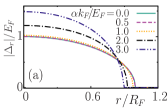
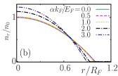
Figure 11: (Color online) The radial (a) order-parameter and (b) number-density profiles at $T=0$ when $E_{b}=0.5E_{F}$. While the radial profiles remain unchanged for $\alpha\lesssim E_{F}/k_{F}$, increasing $\alpha$ eventually increases both the order parameter and the number density at the trap center.

Even though it is not possible to obtain a closed-form analytic expression for the order-parameter and number equations for arbitrary $\alpha$, we perturbatively find $\mu\simeq E_{F}-E_{b}/2-M\alpha^{2}$ and $|\Delta_{r}|\simeq\Delta_{0}\sqrt{1-r^{2}/R_{F}^{2}}$ with $\Delta_{0}=\sqrt{2E_{F}E_{b}}\sqrt{1+2M^{2}\alpha^{4}/3(E_{b}+2E_{F})^{2}}$ in the $M\alpha^{2}\ll E_{b}+2E_{F}$ limit Chen2012 . This suggests that neither $|\Delta_{r}|$ nor $n_{r}$ are affected much by weak Rashba coupling as clearly illustrated in our numerical solutions presented in Figs. 11(a) and 11(b) for $E_{b}=0.5E_{F}$ and $\alpha\lesssim 1E_{F}/k_{F}$. Increasing $\alpha$ energetically favors more and more the finite-angular-momentum states in the $-$ branch leading to an increased low-energy LDOS. When $M\alpha^{2}\sim E_{b}+2E_{F}$, we see that the monotonic contraction of the gas towards the trap center with $R_{O}<R_{F}$, which is similar to what happens in the non-interacting case, monotonically increases $|\Delta_{r}|$. Thus, the Rashba coupling alone enhances pairing in general, and the entire gas remains to be a disk-shaped SF with gapped excitations.

IV.3 Trapped Fermi gas with adiabatic rotation
($\omega\neq 0$, $\alpha=0$ and $\Omega\neq 0$)

Another analytically-tractable limit is a 2D Fermi gas with adiabatic rotation, for which case the main effect of this coupling is to break some of the Cooper pairs that are made of time-reversed particles within the BCS mean-field approximation for pairing. Note that since the vortices are assumed not to be excited by rotation and that the gapped SF cannot carry any angular momentum, these broken pairs carry the extra angular momentum.

The pair-breaking mechanism is based on the Coriolis effects and it can be analyzed by looking at the excitation spectra shown in Fig. 12. In the $\Omega\to 0$ limit shown in Fig. 12(a), both the quasi-particle $E_{r\mathbf{k}}=\sqrt{\xi_{r\mathbf{k}}^{2}+|\Delta_{r}|^{2}}-\Omega L_{r\mathbf{k}}^{z}$ and quasi-hole $E^{\prime}_{r\mathbf{k}}=-\sqrt{\xi_{r\mathbf{k}}^{2}+|\Delta_{r}|^{2}}-\Omega L_{r\mathbf{k}}^{z}$ excitation energies are particle-hole symmetric around the zero-energy axis along the $k_{y}$-direction, corresponding to an ideal situation for the formation of Cooper pairs with zero center of mass momentum. On the other hand, while $\Omega\neq 0$ still preserves the particle-hole symmetry, it breaks the symmetry between the time-reversed pairing states $(\mathbf{k},\uparrow;-\mathbf{k},\downarrow)$, leading to asymmetric excitation energies that depend on the direction of momentum as shown in Fig. 12(b). Increasing $\Omega$ increases this asymmetry, and it eventually leads to negative/positive quasi-particle/quasi-hole energies and broken pairs in the ground state, i.e., the $\mathbf{k}$-space regions with $E_{r\mathbf{k}}<0$ and $-E^{\prime}_{r,-\mathbf{k}}>0$ are not occupied by pairs but by single particles. These $\mathbf{k}$-space regions $k_{1}<k<k_{2}$ are found by setting $E_{r\mathbf{k}}=0$, leading to $k_{1,2}^{2}=2M\mu_{r}+2M^{2}\Omega^{2}r^{2}\pm 2M\sqrt{\mathrm{A}_{r}}$ with $\mathrm{A}_{r}=2M\Omega^{2}r^{2}\mu_{r}+M^{2}\Omega^{4}r^{4}-|\Delta_{r}|^{2}.$ Thus, $\mathrm{A}_{r}\geq 0$ is a necessary condition for the emergence of local phases with gapless excitations, i.e., a gapless SF (gSF) or N phase.

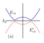
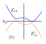
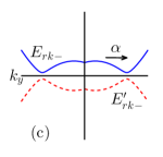
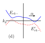
Figure 12: (Color online) Schematic diagrams showing the excitation spectrum $E_{r\mathbf{k}}$ with $\Omega\neq 0$ for (a) a gapped SF at $r=0$ for $\alpha=0$, (b) a gapless SF at $r>0$ for $\alpha=0$, (c) a gapped SF at $r=0$ for $\alpha>0$, and (d) a gapless SF at $r>0$ for $\alpha>0$. The broken Cooper pairs occupy $\mathbf{k}$-space regions with negative/positive quasi-particle/quasi-hole energies.

This LDA analysis suggests that the Cooper pairs are robust for sufficiently slow rotations, and low $\Omega$ has no effect whatsoever on $\mu$, $n_{r}$ and $|\Delta_{r}|$, for which case the entire gas remains to be a disk-shaped SF with gapped excitations, and its edge is located at $R_{O}=R_{F}$. Once the critical rotation frequency $\Omega_{c}$ for the onset of pair breaking is reached, the gapless excitations naturally appear at the edge of the gas, i.e., $\mathrm{A}_{r=R_{F}}=0$, suggesting that the radius of the N gas having the same $\mu$ coincides with the Thomas-Fermi radius at $\Omega_{c}$, i.e., $R_{O}^{0}(\alpha=0,\Omega=\Omega_{c})=R_{F}.$ Thus, transitions from SF to gSF and gSF to N phase first emerge at the edge of the system, and then the SF region contracts toward the trap center as a function of increasing $\Omega$. In contrast to the 3D case, we are able to obtain an analytic expression $\Omega_{c}=\omega\sqrt{E_{b}/(2E_{F})}$ for arbitrary $E_{b}$, and given the upper bound on $\Omega\leq\omega$, it follows that pairs are robust against rotation for $E_{b}>2E_{F}$. The fact that $\mu$ also changes sign at $E_{b}=2E_{F}$ is not a lucky coincidence, since the pairs are known to be robust for $\mu<0$ in earlier works on a 3D Fermi gas Urban2008 ; Iskin2009 .

When $\Omega>\Omega_{c}$, we reach a generic conclusion that the trap profile consists of three regions, where the central SF core and the outer N edge are connected by a coexistence region gSF phase in between. Unlike the N region where $|\Delta_{r}|=0$ and the associated mass-current density $J^{\theta}_{r}=Mn_{r}\Omega r$ is exactly of the form of a rigidly-rotating gas, the gSF region is characterized by $|\Delta_{r}|>0$ and a partially-rotating gas with $J^{\theta}_{r}<Mn_{r}\Omega r$. While the N region expands both inwards and outwards as a function of increasing $\Omega$, the SF and gSF regions survive around the trap center even in the $\Omega\to\omega$ limit since the trap center is immune to the direct-effects of rotation. We note in passing that sufficiently fast rotations may cause a kink in $n_{r}$ right at the SF-N interface (not shown), which is a direct consequence of the competition between the curvature of $n_{r}$ in the SF region which is not effected by rotation and that of the N region which increases with increasing $\Omega$.

IV.4 Trapped Fermi gas with Rashba coupling and rotation
($\omega\neq 0$, $\alpha\neq 0$ and $\Omega\neq 0$)

Having shown analytically that the Rashba coupling and adiabatic rotation have competing effects on superfluidity, we are ready to discuss the generic case with arbitrary $\Omega\neq 0$ and $\alpha\neq 0$, for which case the main effect of their interplay is to form an outer ring-shaped N edge that is completely phase separated from the central SF core by vacuum. This is clearly a remnant of the characteristic ring-shaped density profile that is found in Sec. III.4 considering a non-interacting Fermi gas.

For a given $\alpha$, since the entire SF gas is robust against rotation up to again a critical $\Omega<\Omega_{c}$, all of the physical quantities remain the same as the $\Omega=0$ case discussed above in Sec. IV.2. Furthermore, the rigidity of the SF phase can also be used to determine $\Omega_{c}$ using the following recipe. We first remark that $\Omega_{c}$ is the lowest $\Omega$ satisfying the inequality condition $R_{O}^{0}(\alpha,\Omega=\Omega_{c})\geq R_{O}(\alpha,\Omega=0),$ i.e., the radius of the rotating N phase becomes equal or greater to the radius of the non-rotating SF phase. Then, we observe that the emergent outer N edge is connected (disconnected) to (from) the SF phase by an intermediate gSF region (vacuum) when this equality (inequality) condition is satisfied. Assuming $\Omega>\Omega_{c}$, the former profile is realized for $\alpha^{2}+2\mu/M>0$ with a non-rotating SF core that is characterized by $|\Delta_{r}|\neq 0$ and $J^{\theta}_{r}=0$ near the trap center, an outer N edge that is characterized by $|\Delta_{r}|=0$ rotating rigidly with $J^{\theta}_{r}=Mn_{r}\Omega r$, and a gSF region in between that is characterized by $|\Delta_{r}|\neq 0$ rotating partially with $J^{\theta}_{r}<Mn_{r}\Omega r$. See Fig. 18(b) for such a trap profile. On the other hand, assuming again $\Omega>\Omega_{c}$, the latter profile may be realized for $\alpha^{2}+2\mu/M<0$ (this condition is necessary but not sufficient) with a non-rotating central SF core and a rigidly-rotating ring-shaped N annulus. See Fig. 10(d) for such a trap profile, where the region with $|\Delta_{r}|=0$ fully overlaps with the one with $J^{\theta}_{r}=Mn_{r}\Omega r$.

Increasing $\Omega$ beyond $\Omega_{c}$ leads ultimately to the complete expulsion of superfluidity from the entire trap at a higher critical rotation frequency $\Omega_{s}$. In contrast to the $\alpha\to 0$ limit discussed in Sec. IV.2 where the trap center remains a SF even at $\Omega=\omega$ thanks to its immunity to the direct-effects of rotation, $\alpha\neq 0$ allows such an expulsion since the ring-shaped N annulus that is formed by broken pairs is energetically more favorable than the gapped SF at the trap center.

Next we calculate the critical rotation frequencies both for the onset of pair breaking and for the complete destruction of superfluidity in the system, and construct extensive phase diagrams and trap profiles for a wide-range of parameter regimes.

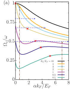
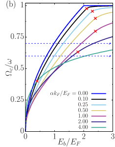
Figure 13: (Color online) The critical rotation frequency for the onset of pair breaking as a function of (a) Rashba coupling, and (b) binding energy at $T=0$. The “x” marks indicate the point beyond which the ring-shaped N annulus emerges disconnectedly from the central SF core by vacuum (see the main text for details). The radial phase profiles along the dashed blue (horizontal) and the dash-dotted brown (vertical) lines in (a) are shown, respectively, in Figs. 15 and 16. Similarly, the radial phase profiles along the dashed blue (horizontal) lines in (b) are shown in Fig. 17.

V Numerical Analysis and Discussion

In comparison to the non-interacting phase diagram presented in Fig. 3, here we show that the complex interplay between Rashba coupling, adiabatic rotation and interaction gives rise to much richer phase diagrams and trap profiles. For the onset of pair breaking and the associated emergence of an outer N edge, the inequality condition discussed above in Sec. IV.4, i.e., $R_{O}^{0}(\alpha,\Omega=\Omega_{c})\geq R_{O}(\alpha,\Omega=0),$ turns out to be a very convenient one for determining $\Omega_{c}$. This is because even though $R_{O}(\alpha,\Omega=0)$ is still obtained through the numerical solutions of the self-consistency equations in this inequality, such an implicit calculation is much more effective than an explicit one requiring self-consistent solutions of the trap profiles in the entire parameter space of interest. For the complete destruction of the central SF core, by noting that this is linked to the depletion of the central density as the trap center is immune to the direct-effects of rotation, solving simultaneously the conditions $n_{r=0}\to 0$ and $\Delta_{\mathbf{r}=0}\to 0$ turns out to be a very convenient approach for determining $\Omega_{s}$. We achieved this by first setting $\Delta_{\mathbf{r}=0}\to 0$ in the order-parameter equation and obtain $\mu$, and then extract $\Omega_{s}$ from the number equation by substituting $\mu$. Let us first construct $\Omega_{c}$ and $\Omega_{s}$ phase diagrams based on these two implicit conditions, and then verify their validity by looking explicitly at the trap profiles.

V.1 Phase diagrams

In Fig. 13, we show $\Omega_{c}$ as a functions of $\alpha$ and $E_{b}$. In contrast to the $\alpha\to 0$ limit discussed in Sec. IV.3 where pairs are shown to be robust against rotation for $E_{b}>2E_{F}$, Fig. 13(a) shows that $\alpha\neq 0$ eventually leads to pair breaking at some $\Omega_{c}$ no matter what $E_{b}$ is. For instance, when $E_{b}\gtrsim 2E_{F}$ as illustrated by the top three curves in this figure, $\Omega_{c}=\omega$ first remains unchanged up to some low but finite $\alpha$ threshold, and then it decreases monotonically as pair breaking starts at lower $\Omega$ with increasing $\alpha$. In this strongly-interacting regime, the outer N edge always emerges disconnectedly from the central SF core by vacuum for $\Omega>\Omega_{c}$.

On the other hand, when $E_{b}\lesssim 2E_{F}$ as illustrated by the bottom three curves in the same figure, $\Omega_{c}$ first decreases up to some critical $\alpha$ threshold, and then it increases with a minimum in between. This is a result of the competing Rashba effects discussed in Sec. IV.2. The dominant effect at low $\alpha$ is that, by shifting the excitation minima to higher momentum states some of which are more susceptible to rotation, the interplay of Rashba coupling and adiabatic rotation makes pair breaking easier. In sharp contrast, increasing $\alpha$ causes two additional effects, i.e., it not only increases $|\Delta_{r}|$ and $n_{r}$ near the trap center but also decreases the radius of the gas, making pair breaking more difficult. Once these latter effects dominate beyond some intermediate $\alpha$ then $\Omega_{c}$ increases with $\alpha$ exhibiting a minimum in between. The location of the minimum shifts to higher $\alpha$ with increased $E_{b}$ as the latter effects become significant only at relatively higher $\alpha$.

Even though it is not possible to obtain a closed-form analytic expression for $\Omega_{c}$ for arbitrary $\alpha$, we approximate the initial drop of $\Omega_{c}$ for low $\alpha$ using the following recipe. By neglecting the secondary effect of Rashba coupling on the radius of the gas, i.e., taking $R_{O}\approx R_{F}$, and inserting $\mu$ that is derived in Sec. IV.2 for a perturbative $\alpha$ into the dispersion relation, the value of $\Omega$ for which the dispersion relation becomes zero at the edge of the gas then gives $\Omega_{c}\approx\omega\sqrt{\alpha^{2}k_{F}^{2}/(2E_{F}^{2})+E_{b}/(2E_{F})}-\omega\alpha k_{F}/(2E_{F}).$ We checked the validity of this expression with the numerical data given in Fig. 13(a), and find an excellent agreement between the two in the low $\alpha$ regime. For even higher values of $\alpha$, since the N edge is favored under adiabatic rotation, it is pushed to longer distances away from the trap center. This changes the mechanism of suppressing the SF phase by directly favoring previously unoccupied unpaired states and alters the behavior of $\Omega_{c}$ curve. Beyond the points marked by “x” in Fig. 13, the curve first goes through a maximum and then decreases with increasing $\alpha$. In this regime, the ring-shaped N annulus emerges disconnectedly from the central SF core by vacuum. Increasing $E_{b}$ lowers the location of this point in the $\alpha$ axis because the condition given above and the fact that $\mu$ decreases with increasing $E_{b}$, in such a way that it ultimately approaches to $\alpha=0$ and $\Omega=\omega$ for $E_{b}\gtrsim 2.5E_{F}$.

In Fig. 13(b), we plot $\Omega_{c}$ as a function of $E_{b}$, showing that $\Omega_{c}$ increases monotonically with $E_{b}$ until it saturates at $\Omega_{c}=\omega$. In addition, we see that increasing $\alpha$ shifts $\Omega_{c}$ curves upwards (downwards) in the low- (high-) $E_{b}$ regime as the Rashba coupling favors (supports) pairing (pair breaking). The points indicated by “x” again mark the critical $E_{b}$ threshold beyond which the ring-shaped N annulus emerges disconnectedly from the central SF core by vacuum. There is only one “x” mark up to $E_{b}\lesssim 2.5E_{F}$, indicating that a gSF region never appears for $E_{b}\gtrsim 2.5E_{F}$. This is in agreement with our analysis given in Sec. IV.4, as the condition $\alpha^{2}+2\mu/M<0$ is satisfied for any $\alpha$ at higher $E_{b}$. However, there are two “x” marks for $E_{b}\sim 2-2.5E_{F}$ at different $\alpha$ values, indicating that while the N region is initially disconnected from the SF one at lower $\alpha$, it first expands with increasing $\alpha$ and connects to the SF with an intermediate gSF region in between, and then it re-disconnects from the SF at a higher $\alpha$. This explains the structure of “x” marks in Fig. 13(b) for $E_{b}\sim 2-2.5E_{F}$ curves, but it is not shown in Fig. 13(a).

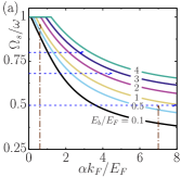
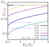
Figure 14: (Color online) The critical rotation frequency for the complete destruction of superfluidity as a function of (a) Rashba coupling, and (b) binding energy at $T=0$. The complete expulsion of SF core from the trap is accompanied by the depletion of the central density, requiring the interplay of Rashba coupling and adiabatic rotation. The horizontal and vertical lines are the same as the ones drawn in Fig. 13.

Lastly, in Fig. 14, we show $\Omega_{s}$ as functions of $\alpha$ and $E_{b}$. Increasing $E_{b}$ shifts $\Omega_{s}$ curves upwards in Fig. 14(a) as the complete destruction of the SF core is expected at higher $\Omega$. In addition, $\Omega_{c}=\omega$ remains unchanged at first up to some low but finite $\alpha$ threshold, and then it decreases monotonically as pair breaking starts at lower $\Omega$ with increasing $\alpha$. This can also be seen in Fig. 14(b), where the critical curves move downward with increasing $\alpha$, and monotonically increase with increasing $E_{b}$. In addition, all of the curves saturate at $\Omega_{s}=\omega$ beyond the critical $E_{b}$ threshold once $E_{b}$ is high enough to protect the pairs against the effects of maximally-allowed rotation frequency $\omega$.

The phase diagrams shown in Figs. 13 and 14 are some of our most important contributions in this paper, as they can be used to predict all sorts of phase profiles in the trap for a wide-range of parameter regimes. Next we demonstrate this along several lines drawn in these figures by directly solving the self-consistency equations for the trap profiles in the entire trap.

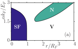
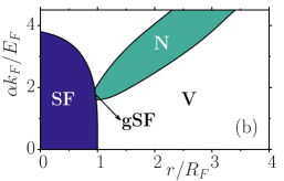
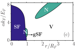
Figure 15: (Color online) Radial phase profiles at $T=0$ with changing Rashba coupling for (a) $E_{b}=3E_{F}$ and $\Omega=0.8\omega$, (b) $E_{b}=2E_{F}$ and $\Omega=0.68\omega$, and (c) $E_{b}=1E_{F}$ and $\Omega=0.5\omega$. Here, the dark blue regions are gapped superfluid (SF), the green regions are normal (N) and the white regions are vacuum (V). The gapless superfluid (gSF) at the SF-N boundaries is not visible on this scale.

V.2 Trap profiles

To demonstrate the practicality of $\Omega_{c}$ and $\Omega_{s}$ phase diagrams shown, respectively, in Figs. 13(a) and 14(a), we first show the resultant phase profiles in Fig. 15 along the dashed blue (horizontal) lines drawn in Figs. 13(a) and 14(a). This figure explicitly shows the emergence and disappearance of N and/or gSF regions in the trap with varying $\alpha$.

For instance, we set $E_{b}=E_{F}$ and $\Omega=0.5\omega$ in Fig. 15(c), corresponding to the bottom horizontal line in Fig. 13(a), and illustrating an exemplary phase profile where the N region appears at the edge of the gas beyond a critical $\alpha$ threshold, as the first intersection point of the bottom horizontal line with $\Omega_{c}$ curve is to the left of the corresponding “x” mark. There is a very thin gSF layer connecting SF and N regions but it is hardly visible in this scale. This $\alpha$ threshold is consistent with the first intersection point of the bottom horizontal line with $\Omega_{c}$ curve in Fig. 13(a). Increasing $\alpha$ in Fig. 15(c) first expands and then contracts the N region. The disappearance of the N edge is due to the interplay of competing Rashba effects discussed in Sec. V.1, and its $\alpha$ threshold is again consistent with the second intersection point of the bottom horizontal line with $\Omega_{c}$ curve. Increasing $\alpha$ further, we see that an N region that is disconnected from central SF core reappears, forming a ring-shaped annulus in the trap, with an increasing width as the SF region is gradually suppressed by $\alpha$. The reappearance $\alpha$ threshold is also consistent with the third intersection point of the bottom horizontal line with $\Omega_{c}$ curve. Lastly, Fig. 15(c) shows that the complete destruction of the SF region occurs beyond $\alpha\approx 8E_{F}/k_{F}$, and its $\alpha$ threshold is again consistent with the intersection points of the bottom horizontal line with $\Omega_{s}$ curve in Fig. 14(a).

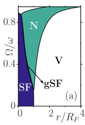
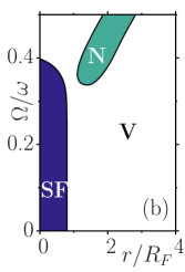
Figure 16: (Color online) Radial phase profiles at $T=0$ with changing rotation frequency for (a) $E_{b}=0.1E_{F}$ and $\alpha=0.6E_{F}/k_{F}$, and (b) $E_{b}=0.1E_{F}$ and $\alpha=7E_{F}/k_{F}$. Here, the dark blue regions are gapped superfluid (SF), the green regions are normal (N) and the white regions are vacuum (V). The gapless superfluid (gSF) at the SF-N boundary is hardly visible in (a) on this scale.

Similarly, we set $E_{b}=2E_{F}$ and $\Omega=0.68\omega$ in Fig. 15(b), corresponding to the middle horizontal line in Fig. 13(a), and illustrating an exemplary phase profile where the N region first appears at the SF edge of the gas beyond a critical $\alpha$ threshold, as the intersection point of the middle horizontal line with $\Omega_{c}$ curve is to the left of the corresponding “x” mark, and then it separates and moves away from the SF region with an increasing width as the SF region is gradually suppressed by $\alpha$. However, we set $E_{b}=3E_{F}$ and $\Omega=0.8\omega$ in the remaining Fig. 15(a), corresponding to the top horizontal line in Fig. 13(a), and illustrating an exemplary phase profile where the N region first appears away from the SF region beyond a critical $\alpha$ threshold, as the intersection point of the top horizontal line with $\Omega_{c}$ curve is to the right of the corresponding “x” mark, and then it moves further away from the SF region with again an increasing width as the SF region is gradually suppressed by $\alpha$. In both of these figures, the $\alpha$ thresholds for the appearance of the N edge are consistent with the only intersection points of the middle/top horizontal lines with $\Omega_{c}$ curves in Fig. 13(a). In addition, the $\alpha$ thresholds for the complete destruction of the SF regions are again consistent with the intersection points of the middle/top horizontal lines with $\Omega_{s}$ curves in Fig. 14(a).

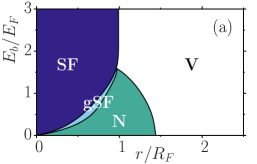
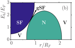
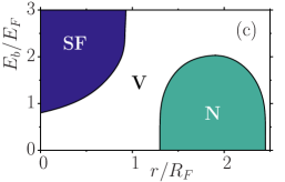
Figure 17: (Color online) Radial phase profiles at $T=0$ with changing binding energy for (a) $\alpha=0.5E_{F}/k_{F}$ and $\Omega=0.7\omega$, (b) $\alpha=2E_{F}/k_{F}$ and $\Omega=0.7\omega$, and (c) $\alpha=4E_{F}/k_{F}$ and $\Omega=0.6\omega$. Here, the dark blue regions are gapped superfluid (SF), the light blue regions are gapless superfluid (gSF) (not visible in (b)), the green regions are normal (N) and the white regions are vacuum (V).

We next verify the consistency of our $\Omega_{c}$ and $\Omega_{s}$ phase diagrams along the dash-dotted brown (vertical) lines drawn in Figs. 13(a) and 14(a) with the resultant phase profiles shown in Fig. 16. This figure explicitly shows the emergence and disappearance of N and/or gSF regions in the trap with varying $\Omega$. For instance, Fig. 16(a) exemplifies the low $\alpha<2E_{F}/k_{F}$ and/or low $E_{b}<2E_{F}$ regimes, where the N and gSF regions appear simultaneously at the edge of the gas at a critical $\Omega$ threshold, as the intersection point of the left vertical line with $\Omega_{c}$ curve is to the left of the corresponding “x” mark, beyond which increasing $\Omega$ ultimately disconnects the N edge from the SF core which is accompanied by the disappearance of the gSF region. However, in the high $\alpha$ and/or high $E_{b}$ regimes, the N region first appears away from the SF region beyond a critical $\Omega$ threshold, as the intersection points of the right vertical line with $\Omega_{c}$ curve is to the right of the corresponding “x” mark, and then the N edge moves further away from the SF region with an increasing width as the SF region is gradually suppressed by $\Omega$. In addition, the $\Omega$ thresholds for the complete destruction of the SF regions are again consistent with the intersection points of the left/right vertical lines with $\Omega_{s}$ curves in Fig. 14(a).

Similarly, to demonstrate the practicality of $\Omega_{c}$ and $\Omega_{s}$ phase diagrams shown, respectively, in Figs. 13(b) and 14(b), we next show the resultant phase profiles in Fig. 17 along the dashed blue (horizontal) lines drawn in Figs. 13(b) and 14(b). This figure explicitly shows the emergence and disappearance of SF and/or gSF regions in the trap with varying $E_{b}$. For instance, Fig. 17(a) exemplifies the low $\alpha$ and/or low $\Omega$ regimes, where the SF and gSF regions appear simultaneously at the trap center at a critical $E_{b}$ threshold, as the intersection point of the top horizontal line with $\Omega_{c}$ curve is to the left of the corresponding “x” mark, beyond which increasing $E_{b}$ ultimately turns the entire gas into a SF, i.e., once $E_{b}$ is high enough to protect all of the pairs against the effects of $\Omega$, which is accompanied by the disappearance of the gSF region. In addition, Fig. 17(a) shows that the complete destruction of the N region occurs beyond $E_{b}\sim 1.6E_{F}$, and its $E_{b}$ threshold is again consistent with the intersection point of the top horizontal line with $\Omega_{c}$ curve in Fig. 13(b). However, in the high $\alpha$ and/or $\Omega$ regimes, the SF region first appears away from the N region beyond a critical $E_{b}$ threshold, as the intersection points of the top horizontal line with $\Omega_{c}$ curve is to the right of the corresponding “x” mark. Note that since the $\alpha$ and $\Omega$ parameters of Figs. 17(b) and 17(c) are above the $\Omega_{c}^{0}(\alpha)$ curve shown in Fig. 3, while the entire gas forms a ring-shaped annulus in the $E_{b}\to 0$ limit, we see that a SF core that is disconnected from the outer N edge appears with an increasing width as the N region is gradually suppressed by $E_{b}$. In addition, the $E_{b}$ thresholds for the complete destruction of the N regions are again consistent with the intersection points of the top/bottom horizontal lines with $\Omega_{c}$ curves in Fig. 13(b).

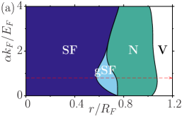
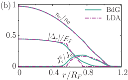
Figure 18: (Color online) (a) Radial phase profiles at $T=0$ with changing Rashba coupling for $E_{b}=0.1E_{F}$ and $\Omega=0.3\omega$. The interplay of Rashba coupling and adiabatic rotation increases the gSF region. (b) An exemplary radial trap profile is plotted along the red dashed line in (a) where $\alpha=0.8E_{F}/k_{F}$, comparing the results of LDA (dot-dashed) and BdG (solid lines, $N=500$) approaches for the order parameter, number density and mass-current density.

We remark here that the interplay between the Rashba coupling and adiabatic rotation may also favor a much wider gSF region in the trap, especially in the low $E_{b}$ regime with an intermediate $\alpha$. For instance, we set $E_{b}=0.1E_{F}$ and $\Omega=0.3\omega$ in Fig. 18(a), illustrating an exemplary phase profile where the emerging gSF region is sandwiched between the central SF core and the outer N edge. In addition, the radial trap profiles are also shown in Fig. 18(b) along the horizontal line drawn in Fig. 18(a), where we compare the results of LDA approach with those of BdG one for $|\Delta_{r}|$, $n_{r}$ and $J_{r}^{\theta}$. Unlike the N region where $|\Delta_{r}|=0$ and the associated $J^{\theta}_{r}=Mn_{r}\Omega r$ is exactly of the form of a rigidly-rotating gas, while the SF region is characterized by $|\Delta_{r}|>0$ and $J^{\theta}_{r}=0$, the gSF region is characterized by $|\Delta_{r}|>0$ and a partially-rotating gas with $J^{\theta}_{r}<Mn_{r}\Omega r$. In comparison to the LDA results, we find that the BdG ones exhibit a somewhat wider gSF region in the trap, but such finite-size effects are expected to become more and more negligible with increasing $N$. See also Sec. IV for further comparison.

Having accomplished our primary objective, i.e., the exploration the trap profiles of a 2D Fermi gas in the presence of a Rashba coupling and under an adiabatic rotation, next we end the paper with a brief summary of our main findings and an outlook for further research.

VI Conclusions and Outlook

To conclude, here we considered a harmonically-trapped 2D Fermi gas in the presence of a Rashba coupling and under an adiabatic rotation. By adopting the BCS mean-field approximation for local pairing, and BdG and LDA approaches for the isotropic trap, we not only extended our earlier LDA analysis to a wider parameter regime but also compare its results with those of BdG approach showing a perfect agreement for the most parts. For instance, we first analyzed a non-interacting system and showed that the competition between the effects of Rashba coupling on the LDOS and the Coriolis effects caused by rotation gives rise to a characteristic ring-shaped density profile that survives at experimentally-accessible temperatures. Furthermore, we also showed that the Rashba splitting of the Landau levels takes the density profiles on a ziggurat shape in the rapid-rotation limit. We then analyzed an interacting system, and studied the pair-breaking mechanism that is induced by the Coriolis effects on superfluidity, where we calculated the critical rotation frequencies both for the onset of pair breaking and for the complete destruction of SF regions in the system. We also constructed extensive phase diagrams consisting of non-rotating gapped SF, partially-rotating gSF and rigidly-rotating N regions, and used these diagrams to predict all sorts of phase profiles in the trap for a wide-range of parameter regimes, where the aforementioned competition may, e.g., favor an outer N edge that is completely phase separated from the central SF core by vacuum.

This problem offers many extensions for future research. For instance, the interplay between Rashba coupling and adiabatic rotation in a population-imbalanced Fermi gas is a promising one, as these systems manifest topologically non-trivial SF phases in the non-rotating limit Zhou2011a . Since a finite population imbalance is analogous to a perpendicular Zeeman field, we expect not only rich spin-polarization textures reminiscent of skyrmions but also diverse density profiles including the formation of successive ring-shaped regions. Another promising direction is to analyze the effects of real- and/or momentum-space anisotropies on the trap profiles, i.e., trapping potential and/or SOC. In the case of an anisotropic SOC, we again expect exotic density profiles including not only the ring-shaped ones with more than one local maxima in general but also isolated pocket-shaped ones (like a cut through the ring-shaped density) in the 1D SOC limit, i.e., an equal-weight combination of Rashba and Dresselhaus couplings.

VII Acknowledgments

This work is supported by the TUBITAK Grant No. 1001-114F232 and BAGEP award of the Turkish Science Academy, and E. D. is partially supported by a TUBITAK-2215 Ph.D. Fellowship.

Appendix A Expansion of BdG equations in a simple-harmonic-oscillator basis

Using the conservation of total angular momentum about the axis of rotation, we first decompose the BdG eigenvectors into $|l|+1/2$ sectors with $|l|\geq 0$, and then expand the wave functions in terms of the angular-momentum basis of a 2D harmonic oscillator as

$$u_{\mathbf{r}\uparrow\eta} = u^{l}_{\mathbf{r}\uparrow\mathfrak{m}}=\sum_{n}u^{l}_{n\uparrow\mathfrak{m}}R_{rn}^{|l|}\mathrm{e}^{\mathrm{i}l\theta},\quad\,\,u_{\mathbf{r}\downarrow\eta}=u^{l+1}_{\mathbf{r}\downarrow\mathfrak{m}}=\sum_{n}u^{l+1}_{n+1\downarrow\mathfrak{m}}R_{rn+1}^{|l|+1}\mathrm{e}^{\mathrm{i}(l+1)\theta},$$ (17)

$$v_{\mathbf{r}\downarrow\eta} = v^{l}_{\mathbf{r}\downarrow\mathfrak{m}}=\sum_{n}v^{l}_{n\downarrow\mathfrak{m}}R_{rn}^{|l|}\mathrm{e}^{\mathrm{i}l\theta},\quad v_{\mathbf{r}\uparrow\eta}=v^{l+1}_{\mathbf{r}\uparrow\mathfrak{m}}=\sum_{n}v^{l+1}_{n+1\uparrow\mathfrak{m}}R_{rn+1}^{|l|+1}\mathrm{e}^{\mathrm{i}(l+1)\theta},$$ (18)

where the harmonic-oscillator wave functions are given by

$$\braket{r\theta}{nl}\equiv R_{rn}^{|l|}\mathrm{e}^{\mathrm{i}l\theta}=(-1)^{(n-|l|)/2}\sqrt{\frac{[(n-|l|)/2]!}{\pi a_{0}^{2}[(n+|l|)/2]!}}e^{il\theta}\left(\frac{r}{a_{0}}\right)^{|l|}e^{-r^{2}/(2a_{0}^{2})}L^{|l|}_{(n-|l|)/2}(r^{2}/a_{0}^{2}).$$ (19)

Here, $a_{0}=1/\sqrt{M\omega}$ with $\hbar=1$ is the characteristic length scale for the harmonic-oscillator, and the associated Laguerre polynomials $L^{|m|}_{n}(x)$ can be generated from the recursion relation

$$L^{|m|}_{n+1}(x)=\frac{1}{n+1}\left[(2n+1+|m|-x)L^{|m|}_{n}(x)-(n+|m|)L^{|m|}_{n-1}(x)\right],$$ (20)

where $n>1$, $L^{|m|}_{0}(x)=1$ and $L^{|m|}_{1}(x)=1+|m|-x$.

Using the orthogonality of the basis states, we obtain the following matrix-eigenvalue equation for each $|l|+1/2$ sector,

$$\sum_{n^{\prime}}\left(\begin{array}[]{cccc}K_{nn^{\prime}}^{l}&S_{n,n^{\prime}+1}^{-,l+1}&0&\Delta_{nn^{\prime}}^{l^{\prime}}\\ S_{n+1,n^{\prime}}^{+,l}&K_{n+1,n^{\prime}+1}^{l+1}&-\Delta_{n+1,n^{\prime}+1}^{l+1}&0\\ 0&-(\Delta_{n+1,n^{\prime}+1}^{l+1})^{*}&-K_{n+1,n^{\prime}+1}^{-l-1}&-S_{n+1,n^{\prime}}^{+,-l}\\ (\Delta_{nn^{\prime}}^{l})^{*}&0&-S_{n,n^{\prime}+1}^{-,-l-1}&-K_{nn^{\prime}}^{-l^{\prime}}\end{array}\right)\left(\begin{array}[]{l}u^{l}_{n^{\prime}\uparrow\mathfrak{m}}\\ u^{l+1}_{n^{\prime}+1\downarrow\mathfrak{m}}\\ v^{l+1}_{n^{\prime}+1\uparrow\mathfrak{m}}\\ v^{l}_{n^{\prime}\downarrow\mathfrak{m}}\end{array}\right)=E^{l}_{\mathfrak{m}}\left(\begin{array}[]{l}u^{l}_{n\uparrow\mathfrak{m}}\\ u^{l+1}_{n+1\downarrow\mathfrak{m}}\\ v^{l+1}_{n+1\uparrow\mathfrak{m}}\\ v^{l}_{n\downarrow\mathfrak{m}}\end{array}\right)$$ (21)

with the matrix elements

$$K_{nn^{\prime}}^{l} = \braket{nl}{K_{\mathbf{r}}-\Omega L^{z}_{\mathbf{r}}}{n^{\prime}l}=[\omega(n+1)-\mu-\Omega l]\delta_{nn^{\prime}},$$ (22)

$$\Delta_{nn^{\prime}}^{l} = \braket{nl}{\Delta_{r}}{n^{\prime}l}=2\pi\int_{0}^{\infty}rdr\Delta_{r}R_{rn}^{|l|}R_{rn^{\prime}}^{|l|},$$ (23)

$$S_{nn^{\prime}}^{-,l} = \frac{\alpha i}{2a_{0}}\braket{nl-1}{S_{\mathbf{r}}}{n^{\prime}l}=\frac{\alpha i}{2a_{0}}\int d^{2}\mathbf{r}R^{|l|-1}_{rn}\mathrm{e}^{-\mathrm{i}(l-1)\theta}S_{\mathbf{r}}R_{rn^{\prime}}^{|l|}\mathrm{e}^{\mathrm{i}l\theta}$$ (24)

$$= \frac{\alpha i}{2a_{0}}[\sqrt{(n^{\prime}+l)/2}\delta_{n,n^{\prime}-1}-\sqrt{(n^{\prime}-l)/2+1}\delta_{n,n^{\prime}+1}]=-S_{n^{\prime}n}^{+,l-1}.$$

Recall that we restrict our numerical calculations to rotationally-symmetric solutions for $\Delta_{r}$. Similarly, expanding the order parameter, number density and mass-current density equations, we obtain

$$\Delta_{r} =g\sum_{l\mathfrak{m}}\left(\sum_{n}u^{l}_{n\uparrow\mathfrak{m}}R_{rn}^{|l|}\sum_{n^{\prime}}v^{*l}_{n^{\prime}\downarrow\mathfrak{m}}R_{rn^{\prime}}^{|l|}h^{l}_{\mathfrak{m}}+\sum_{n}u^{l+1}_{n+1\downarrow\mathfrak{m}}R_{rn+1}^{|l|+1}\sum_{n^{\prime}}v^{*l+1}_{n^{\prime}+1\uparrow\mathfrak{m}}R_{rn^{\prime}+1}^{|l|+1}f^{l}_{\mathfrak{m}}\right),$$ (25)

$$n_{r} =\sum_{l\mathfrak{m}}\left[\left(\left|\sum_{n}u^{l}_{n\uparrow\mathfrak{m}}R_{rn}^{|l|}\right|^{2}+\left|\sum_{n}u^{l+1}_{n+1\downarrow\mathfrak{m}}R_{rn+1}^{|l|+1}\right|^{2}\right)f^{l}_{\mathfrak{m}}+\left(\left|\sum_{n}v^{l+1}_{n+1\uparrow\mathfrak{m}}R_{rn+1}^{|l|+1}\right|^{2}+\left|\sum_{n}v^{l}_{n\downarrow\mathfrak{m}}R_{rn}^{|l|}\right|^{2}\right)h^{l}_{\mathfrak{m}}\right],$$ (26)

$$J^{\theta}_{r} =\sum_{l\mathfrak{m}}\left\{\left(\frac{l}{r}\left|\sum_{n}u^{l}_{n\uparrow\mathfrak{m}}R_{rn}^{|l|}\right|^{2}+\frac{l+1}{r}\left|\sum_{n}u^{l+1}_{n+1\downarrow\mathfrak{m}}R_{rn+1}^{|l|+1}\right|^{2}\right)f^{l}_{\mathfrak{m}}-\left(\frac{l+1}{r}\left|\sum_{n}v^{l+1}_{n+1\uparrow\mathfrak{m}}R_{rn+1}^{|l|+1}\right|^{2}+\frac{l}{r}\left|\sum_{n}v^{l}_{n\downarrow\mathfrak{m}}R_{rn}^{|l|}\right|^{2}\right)h^{l}_{\mathfrak{m}}\right.$$

$$+\left.2M\alpha\left[\left|\sum_{n}(u^{l}_{n\uparrow\mathfrak{m}})^{*}R_{rn}^{|l|}\sum_{n^{\prime}}u^{l+1}_{n^{\prime}+1\downarrow\mathfrak{m}}R_{rn^{\prime}+1}^{|l|+1}\right|f^{l}_{\mathfrak{m}}+\left|\sum_{n}(v^{l}_{n\downarrow\mathfrak{m}})^{*}R_{rn}^{|l|}\sum_{n^{\prime}}v^{l+1}_{n^{\prime}+1\uparrow\mathfrak{m}}R_{rn^{\prime}+1}^{|l|+1}\right|h^{l}_{\mathfrak{m}}\right]\right\},$$ (27)

where $f^{l}_{\mathfrak{m}}=1-h^{l}_{\mathfrak{m}}=f(E_{\mathfrak{m}}^{l})$. These are alternative to the BdG expressions given in the main text.

References

- (1) J. Dalibard, F. Gerbier, G. Juzeliūnas and P. Öhberg, “Colloquium: Artificial gauge potentials for neutral atoms”, Rev. Mod. Phys. 83, 1523 (2011).
- (2) T.L. Ho and C.V. Ciobanu, “Rapidly rotating Fermi gases”, Phys. Rev. Lett. 85, 4648 (2000).
- (3) X.-L. Qi and S.-C. Zhang, “Topological insulators and superconductors”, Rev. Mod. Phys. 83, 1057 (2011).
- (4) J. Sinova, S. O. Valenzuela, J. Wunderlich, C. H. Back, and T. Jungwirth, “Spin Hall effects”, Rev. Mod. Phys. 87, 1213 (2015).
- (5) M. Z. Hasan and C. L. Kane, “Colloquium: Topological insulators”, Rev. Mod. Phys. 82, 3045 (2010).
- (6) C. Zhang, “Spin-orbit coupling and perpendicular Zeeman field for fermionic cold atoms: Observation of the intrinsic anomalous Hall effect”, Phys. Rev. A 82, 021607(R) (2010).
- (7) E. Doko, A. L. Subaşı, and M. Iskin, “Rotating a Rashba-coupled Fermi gas in two dimensions”, Phys. Rev. A 93, 033640 (2016).
- (8) Y.-J. Lin, Jiménez-García, and I. B. Spielman, “Spin–orbit-coupled Bose–Einstein condensates”, Nature 471, 83 (2011).
- (9) J. Y. Zhang, S. C. Ji, Z. Chen, L. Zhang, Z. D. Du, Bo Yan, G. S. Pan, B. Zhao, Y. J. Deng, H. Zhai, S. Chen, and J. W. Pan, “Collective Dipole Oscillations of a Spin-Orbit Coupled Bose-Einstein Condensate”, Phys. Rev. Lett. 109, 115301 (2012).
- (10) P. Wang, Z.-Q. Yu, Z. Fu, J. Miao, L. Huang, S. Chai, H. Zhai, and J. Zhang, “Spin-orbit coupled degenerate Fermi gases”, Phys. Rev. Lett. 109, 095301 (2012).
- (11) L.W. Cheuk, A.T. Sommer, Z. Hadzibabic, T. Yefsah, W.S. Bakr, and M.W. Zwierlein, “Spin-Injection Spectroscopy of a Spin-Orbit Coupled Fermi Gas”, Phys. Rev. Lett. 109, 095302 (2012).
- (12) C. Qu, C. Hamner, M. Gong, C. Zhang, and P. Engels, “Observation of Zitterbewegung in a spin-orbit-coupled Bose-Einstein condensate”, Phys. Rev. A 88, 021604(R) (2013).
- (13) A. J. Olson, S.-J. Wang, R. J. Niffenegger, C.-H. Li, C. H. Greene, and Y. P. Chen, “Tunable Landau-Zener transitions in a spin-orbit-coupled Bose-Einstein condensate”, Phys. Rev. A 90, 013616 (2014).
- (14) N. Goldman, G. Juzelinas, P. Öhberg, and I. B. Spielman, “Light-induced gauge fields for ultracold atoms”, Rep. Prog. Phys. 77, 126401 (2014).
- (15) K. Jiménez-García, L. LeBlanc, R.Williams, M. Beeler, C. Qu, M. Gong, C. Zhang, and I. Spielman, “Tunable Spin-Orbit Coupling via Strong Driving in Ultracold-Atom Systems”, Phys. Rev. Lett. 114, 125301 (2015).
- (16) L. Huang, Z. Meng, P. Wang, P. Peng, S.-L. Zhang, L. Chen, D. Li, Q. Zhou, and J. Zhang, “Experimental realization of two-dimensional synthetic spin–orbit coupling in ultracold Fermi gases”, Nat. Phys. (2016), doi:10.1038/nphys3672.
- (17) J. Ruseckas, G. Juzelinas, P. Öhberg, and M. Fleischhauer, “Non-Abelian gauge potentials for ultracold atoms with degenerate dark states”, Phys. Rev. Lett. 95, 010404 (2005).
- (18) T. Stanescu, C. Zhang, and V. Galitski, “Nonequilibrium spin dynamics in a trapped Fermi gas with effective spin-orbit interactions”, Phys. Rev. Lett. 99, 110403 (2007).
- (19) G. Juzeliūnas, J. Ruseckas and J. Dalibard, “Generalized Rashba-Dresselhaus spin-orbit coupling for cold atoms”, Phys. Rev. A 81, 053403 (2010).
- (20) D. L. Campbell, G. Juzelinas, and I. B. Spielman, “Realistic Rashba and Dresselhaus spin-orbit coupling for neutral atoms”, Phys. Rev. A 84, 025602 (2011).
- (21) Z. F. Xu and L. You, “Dynamical generation of arbitrary spin-orbit couplings for neutral atoms”, Phys. Rev. A 85, 043605 (2012).
- (22) B. M. Anderson, I. B. Spielman, and G. Juzeliūnas, “Magnetically generated spin-orbit coupling for ultracold atoms”, Phys. Rev. Lett. 111, 125301, (2013).
- (23) D. L. Campbell and I. B. Spielman, “Rashba realization: Raman with RF”, New J. Phys. 18, 033035 (2016).
- (24) K. Martiyanov, V. Makhalov, and A. Turlapov, “Observation of a two-dimensional Fermi gas of atoms”, Phys. Rev. Lett. 105, 030404 (2010).
- (25) P. Dyke, E. D. Kuhnle, S. Whitlock, H. Hu, M. Mark, S. Hoinka, M. Lingham, P. Hannaford, and C. J. Vale, “Crossover from 2D to 3D in a weakly interacting Fermi gas”, Phys. Rev. Lett. 106, 105304 (2011).
- (26) B. Fröhlich, M. Feld, E. Vogt, M. Koschorreck, W. Zwerger, and M. Köhl, “Radio-frequency spectroscopy of a strongly interacting two-dimensional Fermi gas”, Phys. Rev. Lett. 106, 105301 (2011).
- (27) M. Feld, B. Fröhlich, E. Vogt, M. Koschorreck, and M. Köhl, “Observation of a pairing pseudogap in a two-dimensional Fermi gas”, Nature 480, 75 (2011).
- (28) A. T. Sommer, L. W. Cheuk, M. J. H. Ku, W. S. Bakr, and M. W. Zwierlein, “Evolution of fermion pairing from three to two dimensions”, Phys. Rev. Lett. 108, 045302 (2012).
- (29) M. G. Ries, A. N. Wenz, G. Zrn, L. Bayha, I. Boettcher, D. Kedar, P. A. Murthy, M. Neidig, T. Lompe, and S. Jochim, “Observation of pair condensation in the quasi-2D BEC-BCS crossover”, Phys. Rev. Lett. 114, 230401 (2015).
- (30) J. Zhou, W. Zhang, and W. Yi, “Topological superfluid in a trapped two-dimensional polarized Fermi gas with spin-orbit coupling”, Phys. Rev. A 84, 063603 (2011).
- (31) S. Takei, C.-H. Lin, B. M. Anderson, and V. Galitski, “Low-density molecular gas of tightly bound Rashba-Dresselhaus fermions”, Phys. Rev. A 85, 023626 (2012).
- (32) L. He and X.-G. Huang, “BCS-BEC crossover in 2D Fermi gases with Rashba spin-orbit coupling”, Phys. Rev. Lett. 108, 145302 (2012).
- (33) M. Gong, G. Chen, S. Jia, and C. Zhang, “Searching for Majorana fermions in 2D spin-orbit coupled Fermi superfluids at finite temperature”, Phys. Rev. Lett. 109, 105302 (2012).
- (34) A. Ambrosetti, G. Lombardi, L. Salasnich, P. L. Silvestrelli, and F. Toigo, “Polarization of a quasi-two-dimensional repulsive Fermi gas with Rashba spin-orbit coupling: A variational study”, Phys. Rev. A 90, 043614 (2014).
- (35) X. Yang and S. Wan, “Phase diagram of a uniform two-dimensional Fermi gas with spin-orbit coupling”, Phys. Rev. A 85, 023633 (2012).
- (36) W. Zhang and W. Yi, “Topological Fulde–Ferrell–Larkin–Ovchinnikov states in spin–orbit-coupled Fermi gases”, Nat. Commun. 4, 2711 (2013).
- (37) M. Iskin, “Spin-orbit-coupling-induced Fulde-Ferrell-Larkin-Ovchinnikov-like Cooper pairing and skyrmion-like polarization textures in optical lattices”, Phys. Rev. A 88, 013631 (2013).
- (38) Ye Cao, Shu-Hao Zou, Xia-Ji Liu, Su Yi, Gui-Lu Long, and Hui Hu, “Gapless Topological Fulde-Ferrell Superfluidity in Spin-Orbit Coupled Fermi Gases”, Phys. Rev. Lett. 113, 115302 (2014).
- (39) J. R. Abo-Shaeer, C. Raman, J. M. Vogels, and W. Ketterle, “Observation of vortex lattices in Bose-Einstein condensates”, Science 292, 476 (2001).
- (40) M. W. Zwierlein and J. R. Abo-Shaeer, A. Schirotzek, C. H. Schunck, W. Ketterle, “Vortices and superfluidity in a strongly interacting Fermi gas”, Nature 435, 1047 (2005).
- (41) I. Bausmerth, A. Recati, and S. Stringari, “Destroying Superfluidity by Rotating a Fermi Gas at Unitarity”, Phys. Rev. Lett. 100, 070401 (2008).
- (42) I. Bausmerth, A. Recati, and S. Stringari, “Unitary polarized Fermi gas under adiabatic rotation”, Phys. Rev. A 78, 063603 (2008).
- (43) M. Urban and P. Schuck, “Pair breaking in rotating Fermi gases”, Phys. Rev. A 78, 011601 (2008).
- (44) M. Iskin and E. Tiesinga, “Rotation-induced superfluid-normal phase separation in trapped Fermi gases”, Phys. Rev. A 79, 053621 (2009).
- (45) H. J. Warringa and A. Sedrakian, “Vortex formation in a rotating two-component Fermi gas”, Phys. Rev. A 84, 023609 (2011).
- (46) H. J. Warringa, “Location of the vortex phase in the phase diagram of a rotating two-component Fermi gas”, Phys. Rev. A 86, 043615 (2012).
- (47) M. Randeria, J. Duan, and L. Shieh, “Bound states, Cooper pairing, and Bose condensation in two dimensions”, Phys. Rev. Lett. 62, 981 (1989).
- (48) L. He and P. Zhuang, “Phase diagram of a cold polarized Fermi gas in two dimensions”, Phys. Rev. A 78, 033613 (2008).
- (49) G. Chen, M. Gong, and C. Zhang, “BCS-BEC crossover in spin-orbit-coupled two-dimensional Fermi gases”, Phys. Rev. A 85, 013601 (2012).