A New Class of Exponential Integrators for Stochastic Differential Equations With Multiplicative Noise

Abstract.

In this paper, we present new types of exponential integrators for Stochastic Differential Equations (SDEs) that take advantage of the exact solution of (generalised) geometric Brownian motion. We examine both Euler and Milstein versions of the scheme and prove strong convergence. For the special case of linear noise we obtain an improved rate of convergence for the Euler version over standard integration methods. We investigate the efficiency of the methods compared with other exponential integrators and show that by introducing a suitable homotopy parameter these schemes are competitive not only when the noise is linear but also in the presence of nonlinear noise terms.

1. Introduction

We develop new exponential integrators for the numerical approximation stochastic differential equations (SDEs) of the following form

(1) $$d\mathbf{u}=\left(A\mathbf{u}+\bf{F}(\mathbf{u})\right)dt+\sum_{i=1}^{m}\left(B_{i}\mathbf{u}+\mathbf{g}_{i}(\mathbf{u})\right)dW_{i}(t),\qquad\mathbf{u}(0)=\mathbf{u}_{0}\in\mathbb{R}^{d}$$

where $W_{i}(t)$ are iid Brownian Motions, $\mathbf{F},\mathbf{g}_{i}:\mathbb{R}^{d}\rightarrow\mathbb{R}^{d}$, and matrices $A,B_{i}\in\mathbb{R}^{dxd}$ satisfy the following zero commutator conditions

$$\left[A,B_{i}\right]=0,\quad\left[B_{j},B_{i}\right]=0\qquad\text{for}\quad i,j=1\ldots m.$$

In the deterministic setting, exponential integrators have proved to be very efficient in the numerical solution of stiff (partial) differential equations when compared to implicit solvers see, for example, the review in [5]. The derivation and usage of exponential integrators in the stochastic setting is still an active research area. Local linearisation methods were first proposed by [13, 2] for SDEs with both additive and multiplicative noise. These methods continue to receive attention, see for example [21, 12] looking at weak approximation and for example [3] on general noise terms. Recently [16] examined mean square stability of exponential integrators for semi-linear stiff SDEs. The method is the same basic one as developed for the space discretisations of SPDEs. For SPDE’s with additive noise, [18] introduced an exponential scheme for stochastic PDEs and was improved upon in [10, 15], Jentzen and co-workers (see for example [10, 8, 9] and references there in) have further extended these results to include more general nonlinearities. There has been less work on exponential integrators with multiplicative noise. Strong convergence of stochastic exponential integrators for SDEs obtained from space discretisation of stochastic partial differential equations (SPDEs) by finite element method is considered in [19] and recently, a higher order exponential integrator of Milstein type has been introduced by Jentzen and Röckner [11].

All the above exponential integrators for SDEs (e.g. arising from the discretisation of the SPDEs) are based on the semi group operator $\mathbf{S}_{t,t_{0}}=\exp((t-t_{0})A)$ obtained from the following linear equation

$$d\mathbf{S}_{t,t_{0}}=A\mathbf{S}_{t,t_{0}}dt,\qquad\mathbf{S}_{t_{0},t_{0}}=I_{d}$$

where $I_{d}$ is unit matrix in $\mathbb{R}^{d\times d}$. For comparison, consider the following two standard exponential integrators for (1) with multiplicative noise: SETD0

(2) $$\mathbf{u}_{n}=e^{\Delta tA}\left(\mathbf{u}_{n}+\mathbf{F}(\mathbf{u}_{n})\Delta t+\sum_{i=1}^{m}\left(B_{i}\mathbf{u}_{n}+\mathbf{g}_{i}(\mathbf{u}_{n})\right)\Delta W_{i,n}\right)$$

and SETD1

(3) $$\mathbf{u}_{n}=e^{\Delta tA}\left(\mathbf{u}_{n}+\sum_{i=1}^{m}\left(B_{i}\mathbf{u}_{n}+\mathbf{g}_{i}(\mathbf{u}_{n})\right)\Delta W_{i,n}\right)+\mathbf{\varphi}(\Delta tA)\mathbf{F}(\mathbf{u}_{n})\Delta t,$$

where

$$\mathbf{\varphi}(A)=A^{-1}\left(\exp(A)-I_{d}\right).$$

These methods are essentially exact for a linear system of ODEs. We extend this approach to take advantage of the known solution of geometric Brownian motion in the numerical approximation. To do this, consider the linear homogeneous matrix differential equation

(4) $$d\mathbf{\Phi}_{t,t_{0}}=A\mathbf{\Phi}_{t,t_{0}}dt+\sum_{i=1}^{m}\ B_{i}\mathbf{\Phi}_{t,t_{0}}dW_{i}(t),\qquad\mathbf{\Phi}_{t_{0},t_{0}}=I_{d}$$

and these new schemes are exact for a class of linear systems of multiplicative SDEs of this form.

In the next section our new exponential integrators for multiplicative noise are derived and the homotopy scheme is also introduced. The main results of strong convergence analysis for the Euler and Milstein versions of the scheme are stated in Section 3 and numerical examples are presented to examine the efficiency of the proposed schemes. For linear noise we obtain a strong rate of $\mathcal{O}(\Delta t)$ convergence for Euler type scheme, improving over standard methods in this case. Section 4 proves strong convergence of $\mathcal{O}(\Delta t)$ for the Milstein version and finally we conclude.

2. Derivation of the methods

Throughout we assume that $T\in(0,\infty)$ is a fixed real number and we have a partition of the time interval $[0,T]$, $0=t_{0}<t_{1}<t_{2}\ldots t_{N}=T$ with constant step size $\Delta t=t_{j+1}-t_{j}$. Let $(\Omega,\mathcal{F},\mathbb{P})$ be a probability space with filtration $({\mathcal{F}_{t}})_{t\in[0,T]}$. Then under suitable assumptions on $\mathbf{F}$ and $\mathbf{g}_{i}$ it is well known that there exists an $\mathcal{F}_{t^{-}}$ adapted stochastic process $u:[0,T]\times\Omega\rightarrow\mathbb{R}^{d}$ satisfying (1), [20, 22, 17]. The linear homogeneous matrix differential equation (4) has the exact solution

$$\mathbf{\Phi}_{t,t_{0}}=\exp\left((A-\frac{1}{2}\sum_{i=1}^{m}B_{i}^{2})(t-t_{0})+\sum_{i=1}^{m}B_{i}(W_{i}(t)-W_{i}(t_{0}))\right).$$

Let $\mathbf{u}(t)$ be the solution of (1) and take $t=t_{n+1}$, $t_{0}=t_{n}$. Then, applying the Ito formula to $\mathbf{Y}(t)=\mathbf{\Phi}_{t,t_{0}}^{-1}\mathbf{u}$, we obtain

(5) $$\mathbf{u}(t_{n+1})=\mathbf{\Phi}_{t_{n+1},t_{n}}\left(\mathbf{u}(t_{n})+\int_{t_{n}}^{t_{n+1}}\mathbf{\Phi}_{s,t_{n}}^{-1}\tilde{f}\left(\mathbf{u}(s)\right)ds\right.\\ +\left.\sum_{i=1}^{m}\int_{t_{n}}^{t_{n+1}}\mathbf{\Phi}_{s,t_{n}}^{-1}\mathbf{g}_{i}(\mathbf{u}(s))dW_{i}(s)\right)$$

where

(6) $$\tilde{\mathbf{f}}(.)=\mathbf{F}(.)-\sum_{i=1}^{m}B_{i}\mathbf{g}_{i}(.).$$

Different treatment of the integrals in (5) leads to different numerical schemes. We examine Euler and Milstein type methods here, although clearly higher order methods, such as Wagner-Platen type schemes (see for example [1]) could be developed.

2.1. Euler Type Exponential Integrators

When we take the following approximation for the stochastic integral

(7) $$\mathbf{\Phi}_{t_{n+1},t_{n}}\int_{t_{n}}^{t_{n+1}}\mathbf{\Phi}_{s,t_{n}}^{-1}\mathbf{g}_{i}(\mathbf{u}(s))dW_{i}(s)\approx\mathbf{\Phi}_{t_{n+1},t_{n}}\mathbf{g}_{i}(\mathbf{u}(t_{n}))\Delta W_{i,n}$$

where $\Delta W_{i,n}=W_{i}(t_{n+1})-W_{i}(t_{n})$, we derive Euler type Exponential Integrators below. For the deterministic integral in (5) we examine three cases.

1. First taking $\mathbf{\Phi}_{t_{n+1},t_{n}}\int_{t_{n}}^{t_{n+1}}\mathbf{\Phi}_{s,t_{n}}^{-1}\tilde{\mathbf{f}}(\mathbf{u}(s))ds\approx\mathbf{\Phi}_{t_{n+1},t_{n}}\tilde{\mathbf{f}}(\mathbf{u}(t_{n}))\Delta t$, we obtain our first method EI0

   $$\mathbf{u}_{n}=\mathbf{\Phi}_{t_{n+1},t_{n}}\left(\mathbf{u}_{n}+\tilde{\mathbf{f}}(\mathbf{u}_{n})\Delta t+\sum_{i=1}^{m}\mathbf{g}_{i}(\mathbf{u}_{n})\Delta W_{i,n}\right).$$

2. If we take $\mathbf{\Phi}_{t_{n+1},s}\int_{t_{n}}^{t_{n+1}}\mathbf{\Phi}_{s,t_{n}}^{-1}\tilde{\mathbf{f}}(\mathbf{u}(s))ds\approx\mathbf{Z}_{t_{n+1},t_{n}}\mathbf{\varphi}(\Delta tA)\tilde{\mathbf{f}}(\mathbf{u}(t_{n}))\Delta t$ where

   $$\mathbf{Z}_{t,s}=\exp\left(-\frac{1}{2}\sum_{i=1}^{m}B_{i}^{2}(t-s)+\sum_{i=1}^{m}B_{i}(W_{i}(t)-W_{i}(s))\right)$$

   then we obtain our second method EI1

   $$\mathbf{u}_{n}=\mathbf{\Phi}_{t_{n+1},t_{n}}\left(\mathbf{u}_{n}+\sum_{i=1}^{m}\mathbf{g}_{i}(\mathbf{u}_{n})\Delta W_{i,n}\right)+\mathbf{Z}_{t_{n+1},t_{n}}\mathbf{\varphi}(\Delta tA)\tilde{\mathbf{f}}(\mathbf{u}_{n})\Delta t.$$

3. Finally with $\mathbf{\Phi}_{t_{n+1},t_{k}}\int_{t_{n}}^{t_{n+1}}\mathbf{\Phi}_{s,t_{n}}^{-1}\tilde{\mathbf{f}}(\mathbf{u}(s))ds\approx\mathbf{\varphi}(\Delta tA)\tilde{\mathbf{f}}(\mathbf{u}(t_{n}))\Delta t$ we get the method EI2

   $$\mathbf{u}_{n}=\mathbf{\Phi}_{t_{n+1},t_{n}}\left(\mathbf{u}_{n}+\sum_{i=1}^{m}\mathbf{g}_{i}(\mathbf{u}_{n})\Delta W_{i,n}\right)+\mathbf{\varphi}(\Delta tA)\tilde{\mathbf{f}}(\mathbf{u}_{n})\Delta t.$$

We compare the accuracy and efficiency of these approximations for different numerical examples in Section 3.1. In Section 2.2 below we use a higher order approximation of the stochastic integral to derive Milstein versions of these scheme. For general noise the schemes EI0, EI1, EI2 all have the same strong rate of convergence as SETD0 in (2) and SETD1 (3) which is $\Delta t^{1/2}$. However, we expect an improvement in the error when the terms in $B_{i}$ dominate $g_{i}$ in the noise. In the special case where $\mathbf{g}_{i}\equiv 0$ we prove, and show numerically, an improvement in the strong rate of convergence to order one.

It should be noted that all the proposed new type integrators reduce to the usual exponential integrators SETD0 and SETD1 when $B_{i}=0$, $i=1\ldots m$. Indeed, it is observed in numerical simulations that SETD schemes may perform better than the new EI schemes when $B_{i}$ are small compared to $\mathbf{g}_{i}$. On the other hand the EI schemes outperform SETD schemes when $B_{i}$ are dominant. We can capture the good properties of both types of methods by introducing a homotopy type parameter $p\in[0,1]$. Let us rewrite (1) as

(8) $$d\mathbf{u}=\left(A\mathbf{u}+\bf{F}(\mathbf{u})\right)dt+\sum_{i=1}^{m}\left(pB_{i}\mathbf{u}+\mathbf{g}_{i}(\mathbf{u})+(1-p)B_{i}\mathbf{u}\right)dW_{i}(t).$$

For example, applying EI0 for this equation, one obtains HomEI0

(9) $$\mathbf{u}_{n}=\mathbf{\Phi}_{t_{n+1},t_{n}}^{p}\left(\mathbf{u}_{n}+\tilde{\mathbf{f}}^{p}(\mathbf{u}_{n})\Delta t+\sum_{i=1}^{m}\mathbf{g}_{i}^{p}(\mathbf{u}_{n})\Delta W_{i,n}\right)$$

where

(10) $$\mathbf{\Phi}_{t_{n+1},t_{n}}^{p}=\exp\left((A-\frac{1}{2}\sum_{i=1}^{m}p^{2}B_{i}^{2})\Delta t+\sum_{i=1}^{m}pB_{i}\Delta W_{i},n\right),$$

(11) $$\mathbf{g}_{i}^{p}(\mathbf{u})=\mathbf{g}_{i}(\mathbf{u})+(1-p)B_{i}\mathbf{u},\quad\text{and }\quad\tilde{\mathbf{f}}^{p}(\mathbf{u})=\mathbf{F}(\mathbf{u})-\sum_{i=1}^{m}pB_{i}\mathbf{g}_{i}^{p}(\mathbf{u}).$$

It is clear that $p=0$ and $p=1$ give SETD0 and EI0 respectively. In Section 3.1 we suggest a fixed formula for $p$ based on the weighting of $B_{i}$ to $\mathbf{g}_{i}$. However, further consideration could be given to an optimal choice of either a fixed $p$ or of a $p$ assigned during the computation by considering weights of the terms in the diffusion coefficient, so that $p(u,B_{i},g_{i})$. We note that unlike Milstein methods, HomEI0 and the other EI methods have the advantage that they do not require the derivative of the diffusion term.

2.2. Milstein type Exponential Integrators

An alternative treatment of (5) is to use the Ito-Taylor expansion of the diffusion term

(12) $$\mathbf{\Phi}_{s,t_{n}}^{-1}\mathbf{g}_{i}(\mathbf{u}(s))=\mathbf{g}_{i}(\mathbf{u}(t_{n}))+\sum_{l=1}^{m}\int_{t_{n}}^{s}\mathbf{\Phi}_{r,t_{n}}^{-1}\mathbf{H}_{i,l}(\mathbf{u}(r))dW_{l}(r)+\int_{t_{n}}^{s}\mathbf{\Phi}_{r,t_{n}}^{-1}\mathbf{Q}_{i}(\mathbf{u}(r))dr$$

where

(13) $$\mathbf{H}_{i,l}(\mathbf{u}(.))=D\mathbf{g}_{i}\left(\mathbf{u}\left(.\right)\right)\left(B_{l}\mathbf{u}\left(.\right)+\mathbf{g}_{l}\left(\mathbf{u}\left(.\right)\right)\right)-B_{l}\mathbf{g}_{i}\left(\mathbf{u}\left(.\right)\right).$$

and $\mathbf{Q}_{i}(.)$ is the vector function in terms of $A,\mathbf{F},D\mathbf{g}_{i},D^{2}\mathbf{g}_{i}$, $B_{l}$ for $i,l=1,...,m$ (which, for ease of presentation, we do not detail here).

By freezing the integrand of stochastic integral at $r=t_{n}$ and dropping the deterministic integral, one obtains the approximation

(14) $$\mathbf{\Phi}_{s,t_{n}}^{-1}\mathbf{g}_{i}(\mathbf{u}(s))=\mathbf{g}_{i}(\mathbf{u}(t_{n}))+\sum_{l=1}^{m}\int_{t_{n}}^{s}\mathbf{H}_{i,l}(\mathbf{u}(t_{n}))dW_{l}(r)+h.o.t$$

Using this approximation, we obtain the Milstein scheme MI0

(15) $$\mathbf{u}_{n+1}=\mathbf{\Phi}_{t_{n+1},t_{n}}\left(\mathbf{u}_{n}+\tilde{\mathbf{f}}(\mathbf{u}_{n})\Delta t+\sum_{i=1}^{m}\mathbf{g}_{i}(\mathbf{u}_{n})\Delta W_{i,n}\right.\\ \left.+\sum_{i=1}^{m}\sum_{l=1}^{m}\mathbf{H}_{i,l}(\mathbf{u}_{n})\int_{t_{n}}^{t_{n+1}}\int_{t_{n}}^{s}dW_{l}(r)dW_{i}(s)\right).$$

We can also introduce a Milstein homotopy type scheme HomMI0 by applying MI0 to (8).

3. Convergence result and numerical examples

We state in this section the strong convergence result for both EI0 and MI0. Proofs are given in Section 4 and we note that the proofs for the other schemes, including those such as (9), are similar. For these proofs we assume a global Lipschitz condition on the drift and diffusion. Tamed version of the methods for more general drift and diffusions can be derived [4]. We let $\|\cdot\|_{2}$ denote the standard Euclidean norm and $\left\lVert\cdot\right\rVert_{L^{2}(\Omega,\mathbb{R}^{d})}^{2}=\mathbb{E}\left[\left\lVert\cdot\right\rVert_{2}^{2}\right]$.

Assumption 1.

There exists a constant $L>0$ such that the linear growth condition holds: for $\mathbf{u}\in\mathbb{R}^{d}$ and $i=1,\ldots,m$

$$\left\lVert\mathbf{F}(\mathbf{u})\right\rVert_{2}^{2}\leq L(1+\left\lVert\mathbf{u}\right\rVert_{2}^{2}),\qquad\left\lVert\mathbf{g}_{i}(\mathbf{u})\right\rVert_{2}^{2}\leq L(1+\left\lVert\mathbf{u}\right\rVert_{2}^{2}),$$

and the global Lipschitz condition holds: for $\mathbf{u},\mathbf{v}\in\mathbb{R}^{d}$, $i=1,\ldots,m$

$$\left\lVert\mathbf{F}(\mathbf{u})-\mathbf{F}(\mathbf{v})\right\rVert_{2}\leq L\left\lVert\mathbf{u}-\mathbf{v}\right\rVert_{2},\qquad\left\lVert\mathbf{g}_{i}(\mathbf{u})-\mathbf{g}_{i}(\mathbf{v})\right\rVert_{2}\leq L\left\lVert\mathbf{u}-\mathbf{v}\right\rVert_{2}$$

First we state the strong convergence result for the Euler type scheme EIO.

Theorem 1.

Let Assumptions 1 hold and let $\mathbf{u}_{n}$ be approximation to the solution of (1) using EI0. For $T>0$, there exists $K>0$ such that

(16) $$\sup_{0\leq t_{n}\leq T}\left\lVert\mathbf{u}(t_{n})-\mathbf{u}_{n}\right\rVert_{L^{2}(\Omega,\mathbb{R}^{d})}\leq K\Delta t^{1/2}.$$

For the Milstein scheme MI0, we impose the following two extra assumptions.

Assumption 2.

The functions $F,\mathbf{g}_{i}:\mathbb{R}^{d}\rightarrow\mathbb{R}^{d}$ are twice continuously differentiable.

Assumption 3.

For the same constant $L$ as in Assumption 1 for $\mathbf{u},\mathbf{v}\in\mathbb{R}^{d}$, $i,l=1,\ldots,m$

$$\left\lVert D\mathbf{g}_{i}(\mathbf{u})\mathbf{g}_{l}(\mathbf{u})-D\mathbf{g}_{i}(\mathbf{v})\mathbf{g}_{l}(\mathbf{v})\right\rVert_{2}\leq L\left\lVert\mathbf{u}-\mathbf{v}\right\rVert_{2}$$

and

$$\left\lVert D\mathbf{g}_{i}(\mathbf{u})B_{l}\mathbf{u}-D\mathbf{g}_{i}(\mathbf{v})B_{l}\mathbf{v}\right\rVert_{2}\leq L\left\lVert\mathbf{u}-\mathbf{v}\right\rVert_{2}.$$

Theorem 2.

Let Assumptions 1, 2 and 3 hold and let $\mathbf{u}_{n}$ be approximation to the solution of (1) using MI0. For $T>0$, there exists $K>0$ such that

(17) $$\sup_{0\leq t_{n}\leq T}\left\lVert\mathbf{u}(t_{n})-\mathbf{u}_{n}\right\rVert_{L^{2}(\Omega,\mathbb{R}^{d})}\leq K\Delta t.$$

Note that from the definition of $\tilde{\mathbf{f}}$ in (6) and $\mathbf{H}_{i,l}$ in (13), these functions also satisfy global Lipschitz and/or continuously differentiability conditions when the corresponding assumptions on $\mathbf{F}$, $\mathbf{g}_{i}$ and $D\mathbf{g}_{i}$ hold. We give the proofs of both these Theorems in Section 4.

Now consider the special case when $\mathbf{g}_{i}\equiv 0$ in (1). Namely, we have the SDE

(18) $$d\mathbf{u}=\left(A\mathbf{u}+\bf{F}(\mathbf{u})\right)dt+\sum_{i=1}^{m}B_{i}\mathbf{u}dW_{i}(t),\qquad\mathbf{u}(0)=\mathbf{u}_{0}\in\mathbb{R}^{d}$$

for which both the numerical schemes EI0 and MI0 reduce to

(19) $$\mathbf{u}_{n}=\mathbf{\Phi}_{t_{n+1},t_{n}}\left(\mathbf{u}_{n}+\mathbf{F}(\mathbf{u}_{n})\Delta t\right).$$

Remark that we can consider (19) as a Lie Trotter splitting of (18). It is straightforward to conclude the following improvement in the convergence rate for EI0.

Corollary 1.

Let Assumption 1 and continuously differentiability condition hold for $\mathbf{F}$ and let $\mathbf{u}_{n}$ denote the approximation to the solution of (18) by (19). For $T>0$, there exists $K>0$ such that

(20) $$\sup_{0\leq t_{n}\leq T}\left\lVert\mathbf{u}(t_{n})-\mathbf{u}_{n}\right\rVert_{L^{2}(\Omega,\mathbb{R}^{d})}\leq K\Delta t.$$

This is a simple consequence of solving the linear SDE exactly, see Section 4.

3.1. Numerical examples

In this section we perform some numerical experiments to illustrate and confirm the orders of the proposed methods. For comparison SETD0, SETD1, Exponential Milstein ExpMIL [11], the classical Milstein [14] are used as well as the semi-implicit Euler–Maruyama scheme (EM).

Example 1: Ginzburg-Landau Equation

Consider the one dimensional equation

(21) $$du(t)=\left(-u+\frac{\sigma}{2}u-u^{3}\right)dt+\sqrt{\sigma}udW(t),\qquad u(0)=u_{0}$$

that has exact solution [14]

(22) $$u(t)=\frac{u_{0}e^{-t+\sqrt{\sigma}W(t)}}{\sqrt{1+2u_{0}^{2}\int_{0}^{t}e^{-2s+2\sqrt{\sigma}W(s)}}}.$$

It should be noted that the drift term satisfies only a one sided global Lipschitz condition and our proposed schemes might need to be tamed to guarantee strong convergence as in [7]. Analysis of taming for these schemes is considered in [4]. Nevertheless, ordinary Monte Carlo simulations reveal the performance of the new schemes and act as a benchmark for SETD1 (see also [11]). In this SDE MI0 and HomMI0 both reduce to EI0 and HomEI0. We compare here the schemes EI0, EI1, EI2 and HomEI0. Note that (21) is linear in the diffusion and hence Corollary 1 holds and we expect first order convergence. This is observed in Figure 1 (a) where we see first order convergence of the methods EI0, EI1 and EI2. In Figure 1 (b) we compare the efficiency of the schemes and observe that EI0 is the most efficient. For the other examples that we consider we now only show results for EI0 and HomEI0.

(a)                                                                  (b)

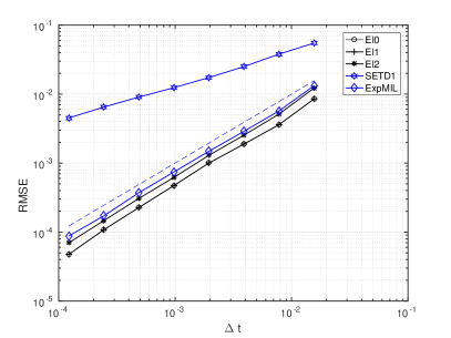
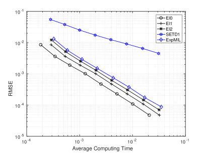
Figure 1. Stochastic Ginzburg-Landau Equation (21) with $\sigma=2$, $T=1$, $M=1000$ samples (a) root mean square error against $\Delta t$. Also plotted is a reference line with slope 1. (b) root mean square error against cputime. Of the new schemes EI0 is the most efficient. We observe the improved convergence rate of Corollary 1 in these new schemes over that for SETD1.

Example 2: nonlinear and non-commutative noise

Consider the following SDE in $\mathbb{R}^{4}$, with initial data $\mathbf{u}(0)=\left(1,1,1,1\right)^{T}$

(23) $$d\mathbf{u}=\left(rA\mathbf{u}+\bf{F}(\mathbf{u})\right)dt+G(\mathbf{u})d\mathbf{W}(t),\qquad F_{j}=\frac{u_{j}}{1+|u_{j}|},$$

where $r$ is a constant (we take $r=4$) and $A$ arises from the standard finite difference approximation of the Laplacian

(24) $$A=\begin{pmatrix}-2&1&0&0\\ 1&-2&1&0\\ 0&1&-2&1\\ 0&0&1&-2\end{pmatrix}.\$$

As we do not have an exact solution in this example we compute a reference solution using the exponential Milstein method with a small step size $\Delta t_{\text{ref}}$ and examine a Monte Carlo estimate of the error $\left\lVert\mathbf{u}(t_{n})-\mathbf{u}_{n}\right\rVert_{L^{2}(\Omega,\mathbb{R}^{d})}$ with $M$ realisations.

Diagonal Noise

First we look at diagonal noise and examine the effective of the noise being dominated by either linear or nonlinear terms. For the nonlinear part we let $g(u)=1/(1+u^{2})$ and let $\mathbf{g}_{i}(\mathbf{u})$ have only one non-zero element $\alpha g(u_{i})$ in the ith entry for $\alpha\in\mathbb{R}$. For the linear part we take $B_{i}=\beta diag(\mathbf{e}_{i})$ where $\mathbf{e}_{i}$ is the ith unit vector of $\mathbb{R}^{4}$ and $\beta\in\mathbb{R}$. This gives $G(u)$ in (23) as

$$G(\mathbf{u})=\begin{pmatrix}\beta u_{1}+\alpha g(u_{1})&0&0\\ 0&\beta u_{2}+\alpha g(u_{2})&0&0\\ 0&0&\beta u_{3}+\alpha g(u_{3})&0\\ 0&0&0&\beta u_{4}+\alpha g(u_{4})\end{pmatrix}\ .$$

When $\alpha<<\beta$ the linear terms $B_{i}$ dominate, whereas if $\alpha>>\beta$, the nonlinearity $\mathbf{g}_{i}$ dominates. By examining different $\alpha$ and $\beta$ we can see the effect of the strength of the nonlinearity. We take $\Delta t_{\text{ref}}=2^{-20}$ and $M=1000$. For HomEI0 and HomMI0 we define the homotopy parameter by

(25) $$p=\dfrac{\mid\beta\mid}{\mid\alpha\mid+\mid\beta\mid}.$$

A matlab script to implement HomEI0 is presented in Algorithm 1. We show results for the both the Euler and Milstein type schemes in each case.

Algorithm 1 Matlab script to solve (23) with noise given by (3) using HomEI0

⬇

1=pow2(10);T=1.0;Dt=T/N;%number of steps,final time,step size

2 d=4;m=4; % dimension of problem and dimension of noise

3 r=4;beta=1;alpha=0.1; % parameters of the problem

4 X=ones(d,1); %initial Condition

5 p=abs(beta)/(abs(beta)+abs(alpha));%set homotopy parameter

6 % Set Matrices

7 A=-r*sparse(toeplitz([2 -1 zeros(1, d-2)])); M1=expm(Dt*A);

8 % Set functions

9 f=@(u) u./(1+abs(u)); g=@(u) 1./(1+u.^2);

10 ftilde=@(u) f(u)-p*beta*(alpha*g(u)+(1-p)*beta*u);

11 Gtilde=@(u) sparse(diag(alpha*g(u)+ (1-p)*beta*u));

12 for n=1:N % loop over time steps

13 dW = sqrt(Dt)*randn(m,1); % get increment for noise

14 M2 = exp(-Dt*0.5*p^2*beta^2+p*beta*dW);

15 X=M1*M2.*(X+Dt*ftilde(X)+Gtilde(X)*dW); % update step

16 end

First consider the case where $\alpha=0.1$ and $\beta=1$ so that the linear term dominate. Figure 2 (a) illustrates orders and (b) the efficiency of the methods EI0, SETD0, HomEI0. In Figure 2 (a) we see convergence with the predicted rate and in Figure 2 (b) it is clear that EI0 and HomEI0 are more efficient than either SETD0 or the semi-implicit Euler–Maruyama method (EM). (Recall that if $\beta=0$ then we obtain first order convergence for EI0 and HomEI0 which is not the case for SETD0 or EM). Figure 3 (a) shows first order convergence for the Milstein schemes and from (b) we see that HomMI0 and MI0 are the most efficient.

(a)                                                                  (b)

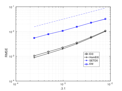
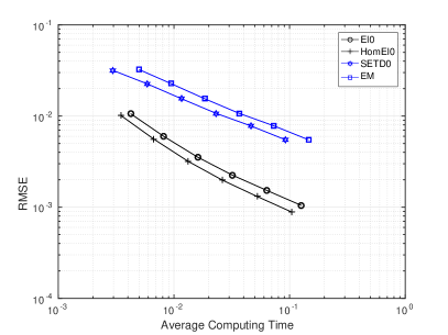
Figure 2. Euler methods. Equation (23) $\beta=1$, $\alpha=0.1$, $r=4$, $T=1$ and $M=1000$ samples (a) root mean square error against $\Delta t$. Also plotted is a reference line with slope 1/2. (b) root mean square error against cputime. Here the linear noise term dominates and we see HomEI0 is the most efficient, followed by EI0. See Figure 3 for Milstein schemes.

(a)                                                                  (b)

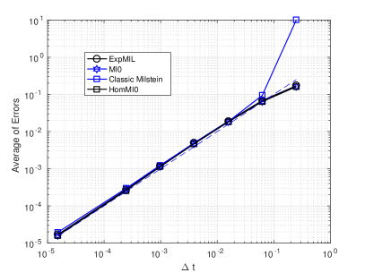
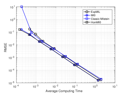
Figure 3. Milstein methods. Equation (23) with $\beta=1$, $\alpha=0.1$, $r=4$, $T=1$ and $M=100$ samples (a) root mean square error against $\Delta t$. Also plotted is a reference line with slope 1 (compare to Figure 2). In (b) root mean square error against cputime. Here the linear noise term dominates and we see HomMI0 and MI0 are the most efficient.

However, when $\beta=\alpha=1$ where we have equal weighting between the linear and nonlinear term we see in Figure 4 (a) the same rate of convergence but now SETD0 and EM are more accurate than EI0. For efficiency we see in Figure 4 (b) that HomEI0 is still the most efficient, followed by SETD0. This illustrates the effectiveness of adding the homotopy parameter. For the Milstein schemes we see the predicted rate of convergence in Figure 5 (a) and in (b) that HomEI0 and MI0 are marginally more efficient than either the classical Milstein or Exponential Milstein schemes.

(a)                                                                  (b)

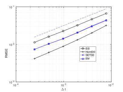
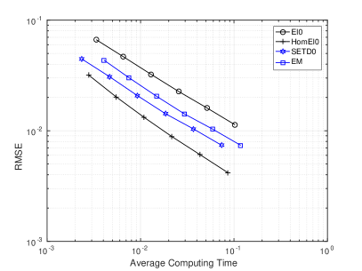
Figure 4. Euler methods. Equation (23) with $\beta=1$, $\alpha=1$, $r=4$, $T=1$ and $M=1000$ samples (a) root mean square error against $\Delta t$. Also plotted is a reference line with slope 1/2. (b) root mean square error against cputime. We have equal weighting of linear and nonlinear noise terms and we see HomEI0 is clearly the most efficient and accurate. See Figure 5 for Milstein type schemes.

(a)                                                                  (b)

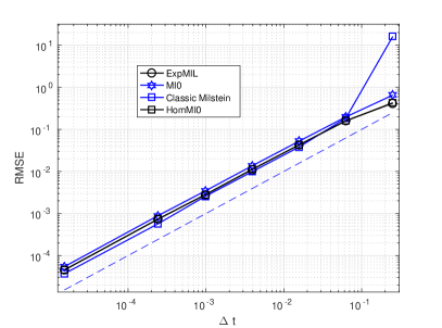
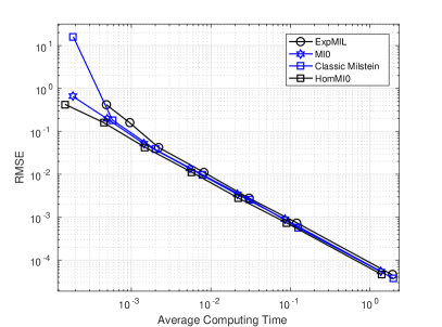
Figure 5. Milstein methods. Equation (23) with $\beta=1$, $\alpha=1$, $r=4$, $T=1$ and $M=100$ samples (a) root mean square error against $\Delta t$. Also plotted is a reference line with slope 1 (compare to Figure 4). In (b) root mean square error against cputime. With equal weighting of the noise we see HomMI0 and MI0 are marginally more efficient.

Next we consider in Figure 6 the case where $\beta=1$ and $\alpha=0.1$ so that it is the nonlinearity that dominates. We now see that the errors from HomEI0 are similar to those or the standard integrators SETD0 and EM and that SETD0 is now more efficient. We note, however, that HomEI0 remains more efficient than EM. For the Milstein schemes we see the predicted rate of convergence in Figure 7 (a) and in (b) that HomEI0 and MI0 are more efficient than either the classical Milstein or Exponential Milstein schemes.

(a)                                                                  (b)

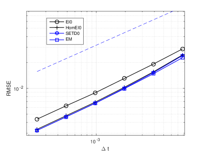
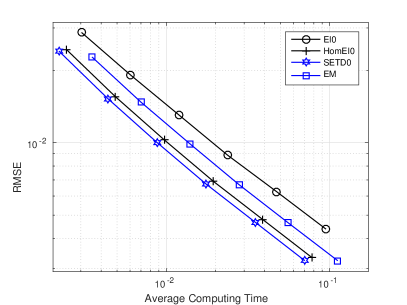
Figure 6. Euler methods. Equation (23) with $\beta=0.1$, $\alpha=1$, $r=4$, $T=1$ and $M=1000$ samples (a) root mean square error against $\Delta t$. Also plotted is a reference line with slope 1/2. (b) root mean square error against cputime. The noise is dominated by the nonlinear term. We now see that SETD0 is the most efficient, followed by HomEI0. See Figure 7 for Milstein type schemes.

(a)                                                                  (b)

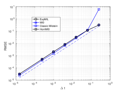
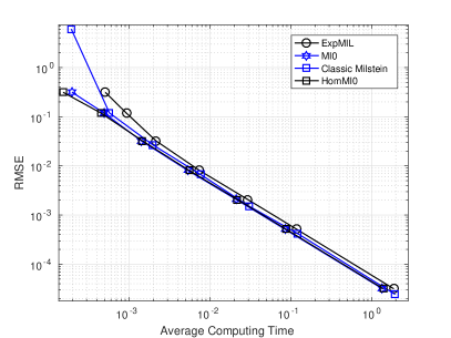
Figure 7. Milstein methods. Equation (23) with $\beta=0.1$, $\alpha=1$, $r=4$, $T=1$ and $M=100$ samples (a) root mean square error against $\Delta t$. Also plotted is a reference line with slope 1 (compare to Figure 6). In (b) root mean square error against cputime. The noise is dominated by the nonlinear term. We see that HomMI0 and MI0 are the most efficient.

Non Commutative Noise

Now consider (23) with non-commutative noise by taking the following diffusion coefficient matrix

(26) $$G(\mathbf{u})=\begin{pmatrix}\beta u_{1}&0&0\\ 0&\beta u_{2}-\alpha u_{1}&0&0\\ 0&0&\beta u_{3}-\alpha u_{2}&0\\ 0&0&0&\beta u_{4}-\alpha u_{3}\end{pmatrix}\$$

In order to apply EI schemes, consider the splitting

(27) $$G(\mathbf{u})=\beta\begin{pmatrix}u_{1}&0&0&0\\ 0&u_{2}&0&0\\ 0&0&u_{3}&0\\ 0&0&0&u_{4}\end{pmatrix}\ -\alpha\begin{pmatrix}0&0&0&0\\ 0&u_{1}&0&0\\ 0&0&u_{2}&0\\ 0&0&0&u_{3}\end{pmatrix}\$$

that gives the matrices $B_{i}=\beta diag(\mathbf{e}_{i})$ and the vectors $\mathbf{g}_{i}(\mathbf{u})$ having only non zero element $-\alpha u_{i}$ in $(i-1)$ th entry. In this case Levy areas are now needed to apply the exponential Milstein scheme and due to this extra computational cost in obtaining a reference solution we reduce the number of samples to $M=100$ and take $\Delta t_{\text{ref}}=2^{-14}$

Figure 8 compares the cases where $\beta=1$, $\alpha=0.1$ in (a) and (b) and $\beta=1$, $\alpha=1$ in (c) and (d). When the linear term dominates Figure 8 (a) and (b) we see that the schemes HomEI0 and EI0 have smaller error and are the most efficient. In Figure 8 (c) and (d), where there is an equal weighting between the diagonal and nondiagonal term in the noise, we see HomEI0 and SETD0 are now equally as efficient. When the nondiagonal part dominates the diagonal part of the noise then Figure 9 shows that HomEI0 is still the most efficient closely followed by the semi-implicit Euler–Maruyama method.

(a)                                                                  (b)

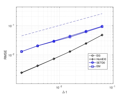
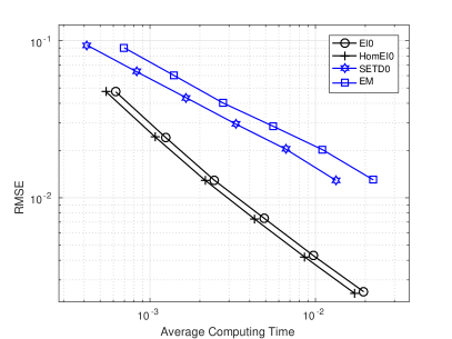
(c)                                                                  (d)

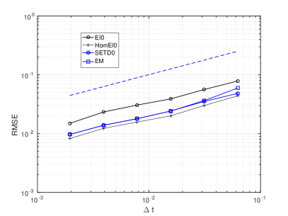
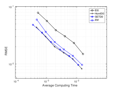
Figure 8. Equation (23) with $r=4$, $T=1$ and $M=1000$ samples comparing in (a), (b) $\beta=1$, $\alpha=0.1$ and in (c), (d) $\beta=1$, $\alpha=1$. (a) and (c) show root mean square error against $\Delta t$. Also plotted is a reference line with slope 1/2. (b) and (d) root mean square error against cputime. Where the diagonal noise term dominates HomEI0 is the most efficient. For equal weighting we see HomEI0 is as efficient as SETD0.

(a)                                                                  (b)

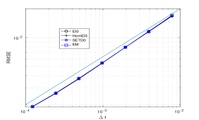
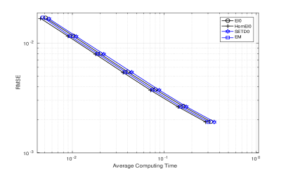
Figure 9. Equation (23) with $r=4$, $T=1$ and $M=1000$ samples with $\beta=0.1$, $\alpha=1$. (a) root mean square error against $\Delta t$. Also plotted is a reference line with slope 1/2. (b) root mean square error against cputime. The noise is dominated by the non diagonal term and we now see that HomEI0 is the most efficient, followed by the semi-implicit Euler–Maruyama method.

Example 3 : Linear stiff SDE

Finally we consider the following linear equation which is used as a test equation for stiff solvers, see for example [23]

(28) $$d\mathbf{u}(t)=\beta\begin{pmatrix}0&1\\ -1&0\end{pmatrix}\mathbf{u}(t)dt+\frac{\sigma}{2}\begin{pmatrix}1&1\\ 1&1\end{pmatrix}\mathbf{u}(t)dW_{1}(t)+\frac{\rho}{2}\begin{pmatrix}1&-1\\ -1&1\end{pmatrix}\mathbf{u}(t)dW_{2}(t)$$

with initial condition $\mathbf{u}(0)=(1,0)^{T}$. The aim is to estimate $\mathbb{E}\left[\mathbf{u}(t)\right]$ for $t\in[0,T]$. It is known from theory that solutions stay in the neighbourhood of the origin, see [23]. We perform simulations with $\beta=5$, $\sigma=4$, $\rho=0.5$ and $T=50$ with a fixed time step of $\Delta t=0.05$ and $M=1000$ realisations. We compare approximations of $\mathbb{E}\left[\mathbf{u}(t)\right]$ using SETD0, and EI0. To apply EI0, we take

(29) $$B_{1}=\frac{\sigma}{2}I_{2},\quad B_{2}=\frac{\rho}{2}I_{2},\quad\mathbf{g}_{1}(\mathbf{u})=\frac{\sigma}{2}\begin{pmatrix}u_{2}\\ u_{1}\end{pmatrix},\quad\mathbf{g}_{2}(\mathbf{u})=\frac{\rho}{2}\begin{pmatrix}-u_{2}\\ -u_{1}\end{pmatrix}.$$

We observe in Figure 10 that the SETD0 solution grows rapidly away from the origin, for EI0 solutions are bounded close to the origin and that the dynamics of EI0 more closely matches the dynamics of the underlying SDE.

(a)                                                                  (b)

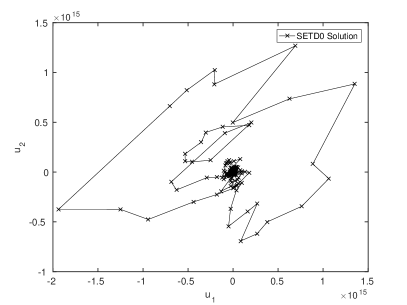
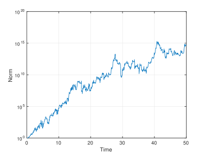
(c)                                                                  (d)

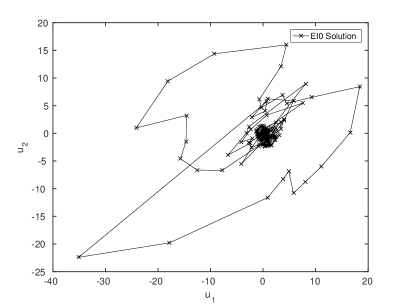
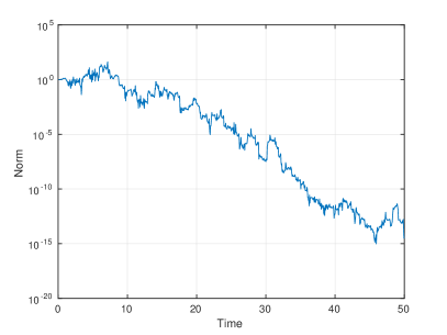
Figure 10. Solution of (28) with $T=50$,$\Delta t=0.05$, $M=1000$. In (a) we plot in the phase place the approximation to $\mathbb{E}\left[\mathbf{u}(t)\right]$ found using SETD0 and in (b) $\|\mathbb{E}\left[\mathbf{u}(t)\right]\|$. In (c) we plot in the phase place the approximation to $\mathbb{E}\left[\mathbf{u}(t)\right]$ found using EI0 and in (d) $\|\mathbb{E}\left[\mathbf{u}(t)\right]\|$. We see that EI0 better captures the true dynamics over this time interval.

4. Proofs of the Main Results

Before giving the proof of main results, we need the following results.

Proposition 1.

Let Assumption 1 hold. For each $T>0$ and $\mathbf{u}(0)=\mathbf{u}_{0}\in\mathbb{R}^{d}$ there exists a unique $\mathbf{u}$ satisfying (1) such that

$$\sup_{t\in[0,T]}\left\lVert\mathbf{u}(t)\right\rVert_{L^{2}(\Omega,\mathbb{R}^{d})}=\sup_{t\in[0,T]}\mathbb{E}\left[\left\lVert\mathbf{u}(t)\right\rVert_{2}^{2}\right]^{1/2}<\infty.$$

Furthermore, there exists $K>0$ such that for $0\leq s,t\leq T$

(30) $$\left\lVert\mathbf{u}(t)-\mathbf{u}(s)\right\rVert_{L^{2}(\Omega,\mathbb{R}^{d})}\leq K|t-s|^{1/2}.$$

See [17] for the proof.

We now examine the remainder terms that arise from the local error. Let us define the map for the exact flow

(31) $$\Psi_{\text{Exact}}(t_{k+1},t_{k},\mathbf{u}(t_{k}))=\\ \mathbf{\Phi}_{t_{k+1},t_{k}}\mathbf{u}(t_{k})+\mathbf{\Phi}_{t_{k+1},t_{k}}\int_{t_{k}}^{t_{k+1}}\mathbf{\Phi}_{s,t_{k}}^{-1}\tilde{\mathbf{f}}(\mathbf{u}(s))ds+\sum_{i=1}^{m}\mathbf{\Phi}_{t_{k+1},t_{k}}\int_{t_{k}}^{t_{k+1}}\mathbf{\Phi}_{s,t_{k}}^{-1}\mathbf{g}_{i}(\mathbf{u}(s))dW_{i}(s).$$

This exact flow will be used in analysis of EI0. However, it is more convenient to use the following Ito-Taylor expansion (see (12)) to analyse MI0

(32) $$\Psi_{\text{Exact}}(t_{k+1},t_{k},\mathbf{u}(t_{k}))=\\ \mathbf{\Phi}_{t_{k+1},t_{k}}\mathbf{u}(t_{k})+\mathbf{\Phi}_{t_{k+1},t_{k}}\int_{t_{k}}^{t_{k+1}}\mathbf{\Phi}_{s,t_{k}}^{-1}\tilde{\mathbf{f}}(\mathbf{u}(s))ds+\sum_{i=1}^{m}\mathbf{\Phi}_{t_{k+1},t_{k}}\int_{t_{k}}^{t_{k+1}}\mathbf{g}_{i}(\mathbf{u}(t_{k}))dW_{i}(s)\\ +\sum_{i=1}^{m}\sum_{l=1}^{m}\mathbf{\Phi}_{t_{k+1},t_{k}}\int_{t_{k}}^{t_{k+1}}\int_{t_{k}}^{s}\mathbf{\Phi}_{r,t_{k}}^{-1}\mathbf{H}_{i,l}(\mathbf{u}(r))dW_{l}(r)dW_{i}(s)\\ +\sum_{i=1}^{m}\mathbf{\Phi}_{t_{k+1},t_{k}}\int_{t_{k}}^{t_{k+1}}\int_{t_{k}}^{s}\mathbf{\Phi}_{r,t_{k}}^{-1}\mathbf{Q}_{i}(\mathbf{u}(r))drdW_{i}(s).$$

The numerical flows for EI0 and MI0 are given by

(33) $$\Psi_{EI0}(t_{k+1},t_{k},\mathbf{u}(t_{k}))=\mathbf{\Phi}_{t_{k+1},t_{k}}\mathbf{u}(t_{k})+\mathbf{\Phi}_{t_{k+1},t_{k}}\int_{t_{k}}^{t_{k+1}}\tilde{\mathbf{f}}(\mathbf{u}(t_{k}))ds\\ +\sum_{i=1}^{m}\mathbf{\Phi}_{t_{k+1},t_{k}}\int_{t_{k}}^{t_{k+1}}\mathbf{g}_{i}(\mathbf{u}(t_{k}))dW_{i}(s)$$

and

(34) $$\Psi_{\mathit{MI0}}(t_{k+1},t_{k},\mathbf{u}(t_{k}))=\mathbf{\Phi}_{t_{k+1},t_{k}}\mathbf{u}(t_{k})+\mathbf{\Phi}_{t_{k+1},t_{k}}\int_{t_{k}}^{t_{k+1}}\tilde{\mathbf{f}}(\mathbf{u}(t_{k}))ds\\ +\sum_{i=1}^{m}\mathbf{\Phi}_{t_{k+1},t_{k}}\int_{t_{k}}^{t_{k+1}}\mathbf{g}_{i}(\mathbf{u}(t_{k}))dW_{i}(s)+\sum_{i=1}^{m}\sum_{l=1}^{m}\mathbf{\Phi}_{t_{k+1},t_{k}}\int_{t_{k}}^{t_{k+1}}\int_{t_{k}}^{s}\mathbf{H}_{i,l}(\mathbf{u}(t_{k}))dW_{l}(r)dW_{i}(s).$$

First we look at the local error $R_{EI0}$ for EI0, where $R_{EI0}$ is defined as

(35) $$R_{EI0}(t,s,\mathbf{u}(s))=\Psi_{\text{Exact}}(t,s,\mathbf{u}(s))-\Psi_{EI0}(t,s,\mathbf{u}(s)).$$

Lemma 1.

Let the Assumptions 1 hold. Then

(36) $$\left\lVert\sum_{k=0}^{N-1}\mathbf{\Phi}_{t_{N},t_{k+1}}R_{EI0}(t_{k+1},t_{k},\mathbf{u}(t_{k}))\right\rVert_{L^{2}(\Omega,\mathbb{R}^{d})}^{2}=\mathcal{O}(\Delta t)$$

Proof.

Considering the exact flow (31) and the numerical flow (33), the local error of EI0 is given by

(37) $$R_{EI0}(t_{k+1},t_{k},\mathbf{u}(t_{k}))=\mathbf{\Phi}_{t_{k+1},t_{k}}\int_{t_{k}}^{t_{k+1}}\left(\mathbf{\Phi}_{s,t_{k}}^{-1}\tilde{\mathbf{f}}(\mathbf{u}(s))-\tilde{\mathbf{f}}(\mathbf{u}(t_{k})\right)ds\\ +\sum_{i=1}^{m}\mathbf{\Phi}_{t_{k+1},t_{k}}\int_{t_{k}}^{t_{k+1}}\left(\mathbf{\Phi}_{s,t_{k}}^{-1}\mathbf{g}_{i}(\mathbf{u}(s))-\mathbf{g}_{i}(\mathbf{u}(t_{k}))\right)dW_{i}(s).$$

Adding and subtracting the terms $\mathbf{\Phi}_{s,t_{k}}^{-1}\tilde{\mathbf{f}}(\mathbf{u}(t_{k})$, $\mathbf{\Phi}_{s,t_{k}}^{-1}\mathbf{g}_{i}(\mathbf{u}(t_{k}))$ in the first and second integrals we have

$$\left\lVert\sum_{k=0}^{N-1}\mathbf{\Phi}_{t_{N},t_{k+1}}R_{EI0}(t_{k+1},t_{k},\mathbf{u}(t_{k}))\right\rVert_{L^{2}(\Omega,\mathbb{R}^{d})}^{2}\leq$$

$$+4\left\lVert\sum_{k=0}^{N-1}\mathbf{\Phi}_{t_{N},t_{k}}\int_{t_{k}}^{t_{k+1}}\mathbf{\Phi}_{s,t_{k}}^{-1}\left(\tilde{\mathbf{f}}(\mathbf{u}(s))-\tilde{\mathbf{f}}(\mathbf{u}(t_{k})\right)ds\right\rVert_{L^{2}(\Omega,\mathbb{R}^{d})}^{2}$$

$$4\left\lVert\sum_{k=0}^{N-1}\mathbf{\Phi}_{t_{N},t_{k}}\int_{t_{k}}^{t_{k+1}}\left(\mathbf{\Phi}_{s,t_{k}}^{-1}\tilde{\mathbf{f}}(\mathbf{u}(t_{k}))-\tilde{\mathbf{f}}(\mathbf{u}(t_{k})\right)ds\right\rVert_{L^{2}(\Omega,\mathbb{R}^{d})}^{2}$$

$$+4\left\lVert\sum_{k=0}^{N-1}\mathbf{\Phi}_{t_{N},t_{k}}\sum_{i=1}^{m}\int_{t_{k}}^{t_{k+1}}\mathbf{\Phi}_{s,t_{k}}^{-1}\left(\mathbf{g}_{i}(\mathbf{u}(s))-\mathbf{g}_{i}(\mathbf{u}(t_{k}))\right)dW_{i}(s)\right\rVert_{L^{2}(\Omega,\mathbb{R}^{d})}^{2}$$

$$+4\left\lVert\sum_{k=0}^{N-1}\mathbf{\Phi}_{t_{N},t_{k}}\sum_{i=1}^{m}\int_{t_{k}}^{t_{k+1}}\left(\mathbf{\Phi}_{s,t_{k}}^{-1}\mathbf{g}_{i}(\mathbf{u}(t_{k}))-\mathbf{g}_{i}(\mathbf{u}(t_{k}))\right)dW_{i}(s)\right\rVert_{L^{2}(\Omega,\mathbb{R}^{d})}^{2}$$

$$=I+II+III+IV.$$

We now consider each of the terms $I$, $II$, $III$, $IV$ separately and we start with $I$

$$I \leq 4N\sum_{k=0}^{N-1}\left\lVert\mathbf{\Phi}_{t_{N},t_{k}}\int_{t_{k}}^{t_{k+1}}\mathbf{\Phi}_{s,t_{k}}^{-1}\left(\tilde{\mathbf{f}}(\mathbf{u}(s))-\tilde{\mathbf{f}}(\mathbf{u}(t_{k})\right)ds\right\rVert_{L^{2}(\Omega,\mathbb{R}^{d})}^{2}$$

$$\leq 4N\sum_{k=0}^{N-1}C_{k}\left\lVert\int_{t_{k}}^{t_{k+1}}\mathbf{\Phi}_{s,t_{k}}^{-1}\left(\tilde{\mathbf{f}}(\mathbf{u}(s))-\tilde{\mathbf{f}}(\mathbf{u}(t_{k})\right)ds\right\rVert_{L^{2}(\Omega,\mathbb{R}^{d})}^{2}$$

$$\leq 4NC\sum_{k=0}^{N-1}\mathbb{E}\left[\left\lVert\int_{t_{k}}^{t_{k+1}}\left(\mathbf{\Phi}_{s,t_{k}}^{-1}\tilde{\mathbf{f}}(\mathbf{u}(s))-\tilde{\mathbf{f}}(\mathbf{u}(t_{k})\right)ds\right\rVert_{2}^{2}\right]$$

where $C=\sup_{k=0,1,2,...N-1}C_{k}$ and $C_{k}$ is due to boundedness of $\mathbf{\Phi}_{t_{N},t_{k}}$ in $L^{2}(\Omega,\mathbb{R}^{d})$. However, in the following lines C is used as a generic constant which may vary from line to line due to boundedness of $\mathbf{\Phi}$ and $\mathbf{\Phi}^{-1}$. Now, Jensen’s inequality, global Lipschitz property of $\tilde{\mathbf{f}}$ and Proposition 1 are applied to get

$$I \leq 4N\Delta tC\sum_{k=0}^{N-1}\int_{t_{k}}^{t_{k+1}}\mathbb{E}\left[\left\lVert\mathbf{\Phi}_{s,t_{k}}^{-1}\left(\tilde{\mathbf{f}}(\mathbf{u}(s))-\tilde{\mathbf{f}}(\mathbf{u}(t_{k})\right)\right\rVert_{2}^{2}\right]ds$$

$$\leq 4TCL^{2}\sum_{k=0}^{N-1}\int_{t_{k}}^{t_{k+1}}\mathbb{E}\left[\left\lVert\left(\mathbf{u}(s)-\mathbf{u}(t_{k})\right)\right\rVert_{2}^{2}\right]ds$$

$$\leq 4TCL^{2}\sum_{k=0}^{N-1}\int_{t_{k}}^{t_{k+1}}|s-t_{k}|ds=K_{I}\Delta t.$$

Similarly, for $II$. It is easy to see $II\leq K_{II}\Delta t$ by considering the fact that $\mathbb{E}\left[\left\lVert\left(\mathbf{\Phi}_{s,t_{k}}^{-1}-I\right)\mathbf{v}\right\rVert_{2}^{2}\right]\leq K|s-t_{k}|$ for any ${\mathcal{F}_{t_{k}}}$ measurable $\mathbf{v}\in L^{2}(\Omega,\mathbb{R}^{d})$, which can be concluded from the Ito-Taylor expansion of $\mathbf{\Phi}_{s,t_{k}}^{-1}\mathbf{v}$. For the term $III$,

$$III=4\left\lVert\mathbf{\Phi}_{t_{N},0}\sum_{k=0}^{N-1}\sum_{i=1}^{m}\int_{t_{k}}^{t_{k+1}}\mathbf{\Phi}_{s,0}^{-1}\left(\mathbf{g}_{i}(\mathbf{u}(s))-\mathbf{g}_{i}(\mathbf{u}(t_{k}))\right)dW_{i}(s)\right\rVert_{L^{2}(\Omega,\mathbb{R}^{d})}^{2}$$

where $\mathbf{\Phi}_{t_{N},t_{k}}=\mathbf{\Phi}_{t_{N},0}\mathbf{\Phi}_{t_{k},0}^{-1}$ is due to commutativity of the matrices $A$ and $B_{i}$’s. We have by the Ito isometry

$$III \leq 4C\sum_{k=0}^{N-1}\sum_{i=1}^{m}\int_{t_{k}}^{t_{k+1}}\mathbb{E}\left[\left\lVert\mathbf{\Phi}_{s,0}^{-1}\left(\mathbf{g}_{i}(\mathbf{u}(s))-\mathbf{g}_{i}(\mathbf{u}(t_{k}))\right)\right\rVert_{2}^{2}\right]ds$$

$$\leq 4CL^{2}\sum_{k=0}^{N-1}K_{III}\int_{t_{k}}^{t_{k+1}}|s-t_{k}|ds=\mathcal{O}(\Delta t)$$

where global Lipschitz property of $\mathbf{g}_{i}$ and Proposition 1 are used. By a similar argument we have $IV=\mathcal{O}(\Delta t)$. Combining $I$, $II$, $III$ and $IV$ we have the result. ∎

We now prove Theorem 1. By induction, we express the approximation of $\mathbf{u}(t_{N})$ by $\mathbf{u}_{N}$ found by EI0 at $t=t_{N}$ as

(38) $$\mathbf{u}_{N}=\mathbf{\Phi}_{t_{N},0}\mathbf{u}_{0}+\sum_{k=0}^{N-1}\mathbf{\Phi}_{t_{N},t_{k}}\int_{t_{k}}^{t_{k+1}}\tilde{\mathbf{f}}(\mathbf{u}_{k})ds+\sum_{k=0}^{N-1}\sum_{i=1}^{m}\mathbf{\Phi}_{t_{N},t_{k}}\int_{t_{k}}^{t_{k+1}}\mathbf{g}_{i}(\mathbf{u}_{k})dW_{i}(s).$$

Due to commutativity of the matrices $A$ and $B_{i}$’s, $\mathbf{\Phi}_{t_{N},t_{k}}=\mathbf{\Phi}_{t_{N},0}\mathbf{\Phi}_{t_{k},0}^{-1}$, the second matrix $\mathbf{\Phi}_{t_{k},0}^{-1}$ can be put inside the stochastic integrals as well as deterministic integral. Now we define the continuous time process $\mathbf{u}_{\Delta t}(t)$ for (38) that agrees with approximation $\mathbf{u}_{k}$ at $t=t_{k}$. By introducing the variable $\hat{t}=t_{k}$ for $t_{k}\leq t<t_{k+1}$,

(39) $$\mathbf{u}_{\Delta t}(t)=\mathbf{\Phi}_{t,0}\mathbf{u}_{\Delta t}(0)+\mathbf{\Phi}_{t,0}\int_{0}^{t}\mathbf{\Phi}_{\hat{s},0}^{-1}\tilde{\mathbf{f}}(\mathbf{u}_{\Delta t}(\hat{s}))ds+\sum_{i=1}^{m}\mathbf{\Phi}_{t,0}\int_{0}^{t}\mathbf{\Phi}_{\hat{s},0}^{-1}\mathbf{g}_{i}(\mathbf{u}_{\Delta t}(\hat{s}))dW_{i}(s).$$

This continuous version has the property that $\mathbf{u}_{\Delta t}(t_{k})=\mathbf{u}_{k}$. By recalling definition of local error, the iterated sum of the exact solution at $t=t_{N}$ is fonud by induction to be

(40) $$\mathbf{u}(t_{N})=\mathbf{\Phi}_{t_{N},0}\mathbf{u}_{0}+\mathbf{\Phi}_{t_{N},0}\int_{0}^{t_{N}}\mathbf{\Phi}_{\hat{s},0}^{-1}\tilde{\mathbf{f}}(\mathbf{u}(\hat{s}))ds\\ +\mathbf{\Phi}_{t_{N},0}\sum_{i=1}^{m}\int_{0}^{t_{N}}\mathbf{\Phi}_{\hat{s},0}^{-1}\mathbf{g}_{i}(\mathbf{u}(\hat{s}))dW_{i}(s)+\sum_{k=0}^{N-1}\mathbf{\Phi}_{t_{N},t_{k+1}}R_{EI0}(t_{k+1},t_{k},\mathbf{u}(t_{k})).$$

Denoting the error by $\mathbf{e}(\hat{t})=\mathbf{u}(\hat{t})-\mathbf{u}_{\Delta t}(\hat{t})$, we see that

$$\left\lVert\mathbf{e}(\hat{t})\right\rVert_{L^{2}(\Omega,\mathbb{R}^{d})}^{2}\leq\left(3\hat{t}CL^{2}+3CmL^{2}\right)\int_{0}^{\hat{t}}\mathbb{E}\left[\left\lVert\mathbf{e}(s)\right\rVert_{2}^{2}\right]ds+3K\Delta t,$$

where $L$ is the largest one of the Lipschitz constants of the functions $\mathbf{g}_{i}$, $\tilde{\mathbf{f}}$. Finally, Gronwall’s inequality completes the proof.

4.1. Proof of Theorem 2

We now examine the local error for MI0, given by (15).

Lemma 2.

Let Assumptions 1 and 2 and 3 hold. Then

(41) $$\left\lVert\sum_{k=0}^{N-1}\mathbf{\Phi}_{t_{N},t_{k}+1}R_{\mathit{MI0}}(t_{k+1},t_{k},\mathbf{u}(t_{k}))\right\rVert_{L^{2}(\Omega,\mathbb{R}^{d})}^{2}=\mathcal{O}(\Delta t^{2})$$

where $R_{\mathit{MI0}}$ is defined as

$$R_{\mathit{MI0}}(t,s,\mathbf{u}(s))=\Psi_{\text{Exact}}(t,s,\mathbf{u}(s))-\Psi_{\mathit{MI0}}(t,s,\mathbf{u}(s)).$$

Proof.

Considering the exact flow (32) and the numerical flow (34) corresponding to the scheme MI0, we have

(42) $$R_{\mathit{MI0}}(t_{k+1},t_{k},\mathbf{u}(t_{k}))=\mathbf{\Phi}_{t_{k+1},t_{k}}\int_{t_{k}}^{t_{k+1}}\left(\mathbf{\Phi}_{s,t_{k}}^{-1}\tilde{\mathbf{f}}(\mathbf{u}(s))-\tilde{\mathbf{f}}(\mathbf{u}(t_{k})\right)ds\\ +\sum_{i=1}^{m}\sum_{l=1}^{m}\mathbf{\Phi}_{t_{k+1},t_{k}}\int_{t_{k}}^{t_{k+1}}\int_{t_{k}}^{s}\left(\mathbf{\Phi}_{r,t_{k}}^{-1}\mathbf{H}_{i,l}(\mathbf{u}(r))-\mathbf{H}_{i,l}(\mathbf{u}(t_{k}))\right)dW_{l}(r)dW_{i}(s)\\ +\sum_{i=1}^{m}\mathbf{\Phi}_{t_{k+1},t_{k}}\int_{t_{k}}^{t_{k+1}}\int_{t_{k}}^{s}\mathbf{\Phi}_{r,t_{k}}^{-1}\mathbf{Q}_{i}(\mathbf{u}(r))drdW_{i}(s).$$

Adding and subtracting the terms $\mathbf{\Phi}_{s,t_{k}}^{-1}\tilde{\mathbf{f}}(\mathbf{u}(t_{k})$, $\mathbf{\Phi}_{s,t_{k}}^{-1}\mathbf{H}_{i,l}(\mathbf{u}(t_{k}))$ in the first and second integrals respectively and summing and taking the norm and applying Jensen’s inequality, we have

$$\left\lVert\sum_{k=0}^{N-1}\mathbf{\Phi}_{t_{N},t_{k+1}}R_{\mathit{MI0}}(t_{k+1},t_{k},\mathbf{u}(t_{k}))\right\rVert_{L^{2}(\Omega,\mathbb{R}^{d})}^{2}\leq I+II+III+IV+V$$

with

$$I:=5\left\lVert\sum_{k=0}^{N-1}\mathbf{\Phi}_{t_{N},t_{k}}\int_{t_{k}}^{t_{k+1}}\mathbf{\Phi}_{s,t_{k}}^{-1}\left(\tilde{\mathbf{f}}(\mathbf{u}(s))-\tilde{\mathbf{f}}(\mathbf{u}(t_{k})\right)ds\right\rVert_{L^{2}(\Omega,\mathbb{R}^{d})}^{2}$$

$$II:=5\left\lVert\sum_{k=0}^{N-1}\mathbf{\Phi}_{t_{N},t_{k}}\int_{t_{k}}^{t_{k+1}}\left(\mathbf{\Phi}_{s,t_{k}}^{-1}\tilde{\mathbf{f}}(\mathbf{u}(t_{k}))-\tilde{\mathbf{f}}(\mathbf{u}(t_{k}))\right)ds\right\rVert_{L^{2}(\Omega,\mathbb{R}^{d})}^{2}$$

$$III:=5\left\lVert\sum_{k=0}^{N-1}\sum_{i=1}^{m}\sum_{l=1}^{m}\mathbf{\Phi}_{t_{N},t_{k}}\int_{t_{k}}^{t_{k+1}}\int_{t_{k}}^{s}\mathbf{\Phi}_{r,t_{k}}^{-1}\left(\mathbf{H}_{i,l}(\mathbf{u}(r))-\mathbf{H}_{i,l}(\mathbf{u}(t_{k}))\right)dW_{l}(r)dW_{i}(s)\right\rVert_{L^{2}(\Omega,\mathbb{R}^{d})}^{2}$$

$$IV:=5\left\lVert\sum_{k=0}^{N-1}\sum_{i=1}^{m}\sum_{l=1}^{m}\mathbf{\Phi}_{t_{N},t_{k}}\int_{t_{k}}^{t_{k+1}}\int_{t_{k}}^{s}\left(\mathbf{\Phi}_{r,t_{k}}^{-1}\mathbf{H}_{i,l}(\mathbf{u}(t_{k}))-\mathbf{H}_{i,l}(\mathbf{u}(t_{k}))\right)dW_{l}(r)dW_{i}(s)\right\rVert_{L^{2}(\Omega,\mathbb{R}^{d})}^{2}$$

and remainder

$$V=:5\left\lVert\sum_{k=0}^{N-1}\sum_{i=1}^{m}\mathbf{\Phi}_{t_{N},t_{k}}\int_{t_{k}}^{t_{k+1}}\int_{t_{k}}^{s}\mathbf{\Phi}_{r,t_{k}}^{-1}\mathbf{Q}_{i}(\mathbf{u}(r))drdW_{i}(s)\right\rVert_{L^{2}(\Omega,\mathbb{R}^{d})}^{2}.$$

We now consider each of the terms $I$, $II$, $III$, $IV$, $V$ separately and we start with $I$. By Assumption 3, we have the following Ito-Taylor expansion for $\tilde{\mathbf{f}}$

$$\tilde{\mathbf{f}}(\mathbf{u(s)}) =\tilde{\mathbf{f}}(\mathbf{u}(t_{k}))+\sum_{i=1}^{m}D\tilde{\mathbf{f}}(\mathbf{u}(t_{k}))\left(B_{i}\mathbf{u}(t_{k})+\mathbf{g}_{i}(\mathbf{u}(t_{k}))\right)\left(W_{i}(s)-W_{i}(t_{k})\right)+R_{\tilde{f}}$$

$$=\tilde{\mathbf{f}}(\mathbf{u}(t_{k}))+\sum_{i=1}^{m}K_{i}\left(W_{i}(s)-W_{i}(t_{k})\right)+R_{\tilde{f}}.$$

We know that $R_{\tilde{f}}=\mathcal{O}(s-t_{k})$, see for example [17]. By Jensen’s inequality for the sum and Ito-Taylor expansion,

$$I\leq 10\mathbb{E}\left[\left\lVert\sum_{k=0}^{N-1}\mathbf{\Phi}_{t_{N},t_{k}}\int_{t_{k}}^{t_{k+1}}\left(\sum_{i=1}^{m}K_{i}\left(W_{i}(s)-W_{i}(t_{k})\right)\right)ds\right\rVert_{2}^{2}\right]$$

$$+10\mathbb{E}\left[\left\lVert\sum_{k=0}^{N-1}\mathbf{\Phi}_{t_{N},t_{k}}\int_{t_{k}}^{t_{k+1}}R_{\tilde{f}}ds\right\rVert_{2}^{2}\right].$$

By boundedness of $\mathbf{\Phi}_{t_{N},t_{k}}$, we have

$$I\leq 10C\mathbb{E}\left[\left\lVert\sum_{k=0}^{N-1}\int_{t_{k}}^{t_{k+1}}\left(\sum_{i=1}^{m}K_{i}\left(W_{i}(s)-W_{i}(t_{k})\right)\right)ds\right\rVert_{2}^{2}\right]+10C\mathbb{E}\left[\left\lVert\sum_{k=0}^{N-1}\int_{t_{k}}^{t_{k+1}}R_{\tilde{f}}ds\right\rVert_{2}^{2}\right].$$

Let us write $I=I_{a}+I_{b}$ and investigate the first term $I_{a}$. By the orthogonality relation $\mathbb{E}\left[<\Theta_{k},\Theta_{l}>\right]=0$, $k\neq l$ for

$$\Theta_{k}=\int_{t_{k}}^{t_{k+1}}\left(\sum_{i=1}^{m}K_{i}\left(W_{i}(s)-W_{i}(t_{k})\right)\right)ds,$$

we have

$$I_{a}=\sum_{k=0}^{N-1}\mathbb{E}\left[\left\lVert\int_{t_{k}}^{t_{k+1}}\left(\sum_{i=1}^{m}K_{i}\left(W_{i}(s)-W_{i}(t_{k})\right)\right)ds\right\rVert_{2}^{2}\right].$$

By two applications of Jensen’s inequality for the integral and sum

$$I_{a}\leq K\Delta t\sum_{k=0}^{N-1}\sum_{i=1}^{m}\int_{t_{k}}^{t_{k+1}}\mathbb{E}\left[\left\lVert W_{i}(s)-W_{i}(t_{k})\right\rVert_{2}^{2}\right]ds=\mathcal{O}(\Delta t^{2}).$$

Since $R_{f}$ contains higher order terms, we conclude $I=\mathcal{O}(\Delta t^{2})$. Similarly, for II we find the same order by following same arguments.

For III, we have by Ito isometry applied consecutively for outer and inner stochastic integrals

$$III\leq$$

$$5C\left\lVert\sum_{k=0}^{N-1}\sum_{i=1}^{m}\sum_{l=1}^{m}\int_{t_{k}}^{t_{k+1}}\int_{t_{k}}^{s}\mathbf{\Phi}_{r,0}^{-1}\left(\mathbf{H}_{i,l}(\mathbf{u}(r))-\mathbf{H}_{i,l}(\mathbf{u}(t_{k}))\right)dW_{l}(r)dW_{i}(s)\right\rVert_{L^{2}(\Omega,\mathbb{R}^{d})}^{2}$$

$$=5C\sum_{k=0}^{N-1}\sum_{i=1}^{m}\int_{t_{k}}^{t_{k+1}}\mathbb{E}\left[\left\lVert\left(\sum_{l=1}^{m}\int_{t_{k}}^{s}\mathbf{\Phi}_{r,0}^{-1}\left(\mathbf{H}_{i,l}(\mathbf{u}(r))-\mathbf{H}_{i,l}(\mathbf{u}(t_{k}))\right)dW_{l}(r)\right)\right\rVert_{2}^{2}\right]ds$$

$$=5C\sum_{k=0}^{N-1}\sum_{i=1}^{m}\sum_{l=1}^{m}\int_{t_{k}}^{t_{k+1}}\int_{t_{k}}^{s}\mathbb{E}\left[\left\lVert\mathbf{\Phi}_{r,0}^{-1}\left(\mathbf{H}_{i,l}(\mathbf{u}(r))-\mathbf{H}_{i,l}(\mathbf{u}(t_{k}))\right)\right\rVert_{2}^{2}\right]drds.$$

By global Lipschitz property of $\mathbf{H}_{i,l}$ and Proposition 1

$$III \leq K_{III}\sum_{k=0}^{N-1}\int_{t_{k}}^{t_{k+1}}\int_{t_{k}}^{s}|r-t_{k}|drds=K_{III}\Delta t^{2}.$$

In a similar way, it can be shown that $IV\leq K_{IV}\Delta t^{2}$. Since $\int_{t_{k}}^{t_{k+1}}\int_{t_{k}}^{s}drdW(s)\sim N(0,\frac{1}{3}\Delta t^{3})$, it is straightforward to see $V\leq K_{V}\Delta t^{2}$.

∎

We now prove Theorem 2. As in the proof of Theorem 1, we define the continuous time process $\mathbf{u}_{\Delta t}(t)$ for MI0 that agrees with approximation $\mathbf{u}_{k}$ at $t=t_{k}$. By introducing the variable $\hat{t}=t_{k}$ for $t_{k}\leq t<t_{k+1}$,

(43) $$\mathbf{u}_{\Delta t}(t)=\mathbf{\Phi}_{t,0}\mathbf{u}_{\Delta t}(0)+\mathbf{\Phi}_{t,0}\int_{0}^{t}\mathbf{\Phi}_{\hat{s},0}^{-1}\tilde{\mathbf{f}}(\mathbf{u}_{\Delta t}(\hat{s}))ds+\sum_{i=1}^{m}\mathbf{\Phi}_{t,0}\int_{0}^{t}\mathbf{\Phi}_{\hat{s},0}^{-1}\mathbf{g}_{i}(\mathbf{u}_{\Delta t}(\hat{s}))dW_{i}(s)\\ +\sum_{i=1}^{m}\sum_{l=1}^{m}\mathbf{\Phi}_{t,0}\int_{0}^{t}\int_{\hat{s}}^{s}\mathbf{\Phi}_{\hat{s},0}^{-1}\mathbf{H}_{i,l}(\mathbf{u}_{\Delta t}(\hat{s}))dW_{l}(r)dW_{i}(s).$$

The iterated sum of the exact solution at $t=t_{N}$ is obtained inductively to be

(44) $$\mathbf{u}(t_{N})=\mathbf{\Phi}_{t_{N},0}\mathbf{u}_{0}+\mathbf{\Phi}_{t_{N},0}\int_{0}^{t_{N}}\mathbf{\Phi}_{\hat{s},0}^{-1}\tilde{\mathbf{f}}(\mathbf{u}(\hat{s}))ds+\mathbf{\Phi}_{t_{N},0}\sum_{i=1}^{m}\int_{0}^{t_{N}}\mathbf{\Phi}_{\hat{s},0}^{-1}\mathbf{g}_{i}(\mathbf{u}(\hat{s}))dW_{i}(s)\\ +\sum_{i=1}^{m}\sum_{l=1}^{m}\mathbf{\Phi}_{t_{N},0}\int_{0}^{t_{N}}\int_{\hat{s}}^{s}\mathbf{\Phi}_{\hat{s},0}^{-1}\mathbf{H}_{i,l}(\mathbf{u}(\hat{s}))dW_{l}(r)dW_{i}(s)+\sum_{k=0}^{N-1}\mathbf{\Phi}_{t_{N},t_{k+1}}R_{\mathit{MI0}}(t_{k+1},t_{k},\mathbf{u}(t_{k}))$$

Denoting the error by $\mathbf{e}(\hat{t})=\mathbf{u}(\hat{t})-\mathbf{u}_{\Delta t}(\hat{t})$, we see that

(45) $$\left\lVert\mathbf{e}(\hat{t})\right\rVert_{L^{2}(\Omega,\mathbb{R}^{d})}^{2}\leq\left(4\hat{t}CL^{2}+4CL^{2}m(1+m)\right)\int_{0}^{\hat{t}}\mathbb{E}\left[\left\lVert\mathbf{e}(s)\right\rVert_{2}^{2}\right]ds+4K\Delta t^{2}.$$

Finally, Gronwall’s inequality completes the proof.

5. Conclusion and Remarks

Exponential integrators that take advantage of Geometric Brownian Motion have been derived and their strong convergence properties discussed. Furthermore we introduced a homotopy based scheme that can take advantage of linearity in the diffusion and also effectively handle nonlinear noise. The proposed schemes are particularly well suited to the SDEs arising from the semi-discretisation of a SPDE where typically diagonal noise arises. Where the SDEs are not of the semi-linear form of (1) then a Rosenbrock type method could be applied, similar to [6]. As mentioned in Section 3 the exponential integrators suggest new forms of taming coefficients for for SDEs with non globally Lipschitz drift and diffusion terms [7], see [4]. Our numerical examples show that these new exponential based schemes are more efficient than the standard integrators and also deal well with the stiff linear problem. In addition we see the effectiveness of the homotopy approach with the simple choice of parameter in (25), (it would be interesting to investigate an adaptive choice in the future).

References

- [1] S. Becker, A. Jentzen, and P. Kloeden. An exponential Wagner–Platen type scheme for spdes. SIAM J. Numer. Anal., 2016.
- [2] R Biscay, JC Jimenez, JJ Riera, and PA Valdes. Local linearization method for the numerical solution of stochastic differential equations. Annals of the Institute of Statistical Mathematics, 48(4):631–644, 1996.
- [3] F. Carbonell and J. C. Jimenez. Weak local linear discretizations for stochastic differential equations with jumps. J. Appl. Probab., 45(1):201–210, 2008.
- [4] Utku Erdogan and Gabriel J Lord. Tamed exponential integrators for stochastic differenatial equations. In Preparation.
- [5] Marlis Hochbruck and Alexander Ostermann. Exponential integrators. Acta Numerica, 19:209–286, 2010.
- [6] Marlis Hochbruck, Alexander Ostermann, and Julia Schweitzer. Exponential rosenbrock-type methods. SIAM Journal on Numerical Analysis, 47(1):786–803, 2009.
- [7] Martin Hutzenthaler and Arnulf Jentzen. Numerical approximations of stochastic differential equations with non-globally Lipschitz continuous coefficients, volume 236. American Mathematical Society, 2015.
- [8] Arnulf Jentzen. Pathwise numerical approximation of SPDEs with additive noise under non-global Lipschitz coefficients. Potential Anal., 31(4):375–404, 2009.
- [9] Arnulf Jentzen. Taylor expansions of solutions of stochastic partial differential equations. Discrete Contin. Dyn. Syst. Ser. B, 14(2):515–557, 2010.
- [10] Arnulf Jentzen and Peter E. Kloeden. Overcoming the order barrier in the numerical approximation of stochastic partial differential equations with additive space-time noise. Proc. R. Soc. Lond. Ser. A Math. Phys. Eng. Sci., 465(2102):649–667, 2009.
- [11] Arnulf Jentzen and Michael Röckner. A Milstein scheme for SPDEs. Foundations of Computational Mathematics, 15(2):313–362, 2015.
- [12] J. C. Jimenez and F. Carbonell. Convergence rate of weak local linearization schemes for stochastic differential equations with additive noise. J. Comput. Appl. Math., 279:106–122, 2015.
- [13] JC Jimenez, I Shoji, and T Ozaki. Simulation of stochastic differential equations through the local linearization method. a comparative study. Journal of Statistical Physics, 94(3-4):587–602, 1999.
- [14] P.E. Kloeden and E. Platen. Numerical Solution of Stochastic Differential Equations. Stochastic Modelling and Applied Probability. Springer Berlin Heidelberg, 2011.
- [15] Peter E Kloeden, Gabriel J Lord, Andreas Neuenkirch, and Tony Shardlow. The exponential integrator scheme for stochastic partial differential equations: Pathwise error bounds. Journal of Computational and Applied Mathematics, 235(5):1245–1260, 2011.
- [16] Yoshio Komori and Kevin Burrage. A stochastic exponential Euler scheme for simulation of stiff biochemical reaction systems. BIT, 54(4):1067–1085, 2014.
- [17] Gabriel J Lord, Catherine E Powell, and Tony Shardlow. An Introduction to Computational Stochastic PDEs. Number 50. Cambridge University Press, 2014.
- [18] Gabriel J Lord and Jacques Rougemont. A numerical scheme for stochastic pdes with Gevrey regularity. IMA journal of numerical analysis, 24(4):587–604, 2004.
- [19] Gabriel J Lord and Antoine Tambue. Stochastic exponential integrators for the finite element discretization of SPDEs for multiplicative and additive noise. IMA Journal of Numerical Analysis, page drr059, 2012.
- [20] Xuerong Mao. Stochastic differential equations and their applications. Horwood Publishing Series in Mathematics & Applications. Horwood Publishing Limited, Chichester, 1997.
- [21] Carlos M. Mora. Weak exponential schemes for stochastic differential equations with additive noise. IMA J. Numer. Anal., 25(3):486–506, 2005.
- [22] Bernt Øksendal. Stochastic differential equations. In Stochastic differential equations, pages 65–84. Springer, 2003.
- [23] V Reshniak, AQM Khaliq, DA Voss, and G Zhang. Split-step Milstein methods for multi-channel stiff stochastic differential systems. Applied Numerical Mathematics, 89:1–23, 2015.