Narrow C iv  absorption doublets on quasar spectra of the Baryon Oscillation Spectroscopic Survey

Abstract

In this paper, we extend our works of Papers I and II (Chen et al., 2014a, b), which are assigned to systematically survey C iv$\lambda\lambda$1548,1551 narrow absorption lines (NALs) with $z_{\rm abs}$$\ll$$z_{\rm em}$ on quasar spectra of the Baryon Oscillation Spectroscopic Survey (BOSS), to collect C iv  NALs with $z_{\rm abs}$$\approx$$z_{\rm em}$ from blue to red wings of C iv$\lambda$1549 emission lines. Together with Papers I and II, we have collected a total number of 41,479 C iv  NALs with $1.4544\leq$$z_{\rm abs}$$\leq 4.9224$ in surveyed spectral region redward of Ly $\alpha$  until red wing of C iv$\lambda$1549 emission line. We find that the stronger C iv  NALs tend to be the more saturated absorptions, and associated systems ($z_{\rm abs}$$\approx$$z_{\rm em}$) seem to have larger absorption strengths when compared to intervening ones ($z_{\rm abs}$$\ll$$z_{\rm em}$). The redshift density evolution behavior of absorbers (the number of absorbers per redshift path) is similar to the history of the cosmic star formation. When compared to the quasar-frame velocity ($\beta$) distribution of Mg ii absorbers, the $\beta$ distribution of C iv  absorbers is broader at $\beta\approx 0$, shows longer extended tail, and exhibits a larger dispersion for environmental absorptions. In addition, for associated C iv  absorbers, we find that low-luminosity quasars seem to exhibit smaller $\beta$ and stronger absorptions when compared to high-luminosity quasars.

1 Introduction

The circumgalactic medium (CGM) surrounding galaxies is crucial to comprehending the feedback from and gas accretion into central objects, as well as galaxy evolution. In recent years, there are a number of successful results of directly detecting emission lines arising from CGM by deep imaging or spectroscopy observations Martin et al. (2014); Hennawi & Prochaska (2013); Cantalupo et al. (2014); Husband et al. (2015); Hennawi et al. (2015); Martin et al. (2015); Arrigoni Battaia et al. (2016). However, it is still difficult to systematically survey the emission of CGM due to the low gas density. Luckily, the CGM would leave marks (so called absorption features) on the spectra of the background objects, which is an efficient way to investigate the properties and kinematics of CGM.

The gas, which infalls from the intergalatic medium (IGM) into galaxies to fuel star formation and is evaporated from galaxies to enrich the metal abundance of IGM, can be well characterized by metal absorption lines (Springel & Hernquist, 2003; Dekel et al., 2009; Richter, 2012; Davé, Finlator, & Oppenheimer, 2012; Rubin et al., 2012; Bouché et al., 2013; Ford et al., 2014; Borthakur et al., 2015; Kacprzak et al., 2015; Nielsen et al., 2015; Muzahid et al., 2015, e.g.,). The cold gas with $T\rm\sim 10^{4}$ — $\rm 10^{5}~{}K$ of CGM has been explored by various transitions from neutral hydrogen to high-ionization absorption lines, such as the absorptions of Ly $\alpha$  (e.g., Kollmeier et al., 2006; Balashev et al., 2014), Ca ii$\lambda\lambda$3934,3969 (e.g., Zhu & Ménard, 2013; Murga et al., 2015), Mg ii$\lambda\lambda$2798,2803 (e.g., Kacprzak et al., 2011; Farina et al., 2014; Huang et al., 2016), Si iii$\lambda$1206 (e.g., Keeney et al., 2013), Si iv$\lambda\lambda$1393,1402 (e.g., Songaila, 2005; Cooksey et al., 2011), C iv$\lambda\lambda$1548,1551 (e.g., Cen & Chisari, 2011; Burchett et al., 2013), N v$\lambda\lambda$1239,1242 (e.g., Fox et al., 2007, 2009; Fechner & Richter, 2009), and O vi$\lambda\lambda$1031,1037 (e.g., Tripp et al., 2008, 2011; Savage et al., 2014). The properties of absorbers (e.g., ionization state, strength, kinematics) are related to halo mass of galaxy, locations and distances between the center of galaxy and absorber, colors, types, luminosities, morphologies, inclination angles, and star formation rates (e.g., Kacprzak et al., 2007, 2015; Gauthier & Chen, 2011; Ford et al., 2014; Farina et al., 2014; Muzahid et al., 2015). Thus, absorption lines provide key insight into galaxy’s CGMs, feedback from central objects, evolutions as well as intrinsic properties of host galaxies.

Outflows and/or jets are fundamental components of active galactic nucleus (AGNs), which play a role in the galaxy evolution by the form of feedback. They carry angular momentum, energy and huge amounts of material away from production sites into host galaxies, CGMs and even IGMs to regulate their star formation rate, metallicities, and element distributions. The outflows are often detected via blueshifted absorption lines. Broad absorption lines (BALs) imprinted on quasar spectra are undoubtedly intrinsic to quasar systems and are likely to be formed in quasar outflows. Narrow absorption lines (NALs) with line widths of a few hundreds $\rm km\,s^{-1}$ are very common on quasar spectra. Some previous studies (e.g., Lü, Qin, & Gupta, 2007; Vanden Berk et al., 2008; Shen & Ménard, 2012; Pan & Chen, 2013) have revealed that a part of NALs with $z_{\rm abs}$$\rm\approx$ $z_{\rm em}$ is also intrinsic to quasar systems. Variation analysis of NALs suggests that some of NALs are probably produced in quasar outflows (e.g., Wise et al., 2004; Narayanan et al., 2004; Chartas et al., 2009; Hamann et al., 2011; Chartas et al., 2012; Chen et al., 2013, 2015). And also, NALs are more common than BALs on quasar spectra especially for Mg ii, because i) low ionization BALs (LoBALs) are rare, and ii) a significant fraction of Mg ii NALs are formed in intervening absorbers (i.e., not physically related to quasar themselves). Therefore, taking full advantage of NALs is crucial to understanding quasar outflows and their influences on surrounding environment.

The Sloan Digital Sky Survey (SDSS, York et al., 2000) is a widely ambitious and influential survey in the astronomical history, which used a dedicated 2.5-meter telescope (Gunn et al., 2006) at Apache Point Observatory, New Mexico, to obtain optical spectra with coverage from $\rm\lambda=3800$ — 9200Å at a resolution of $\rm R\approx 2000$ (Abazajian et al., 2009) during the first (SDSS-I, 2000-2005) and second (SDSS-II, 2005-2008) stages. Some groups (e.g., Nestor, Turnshek, & Rao, 2005; Quider et al., 2011; Zhu & Ménard, 2013; Cooksey et al., 2013; Seyffert et al., 2013) have systematically survey NALs on quasar spectra of the SDSS-I/II. However, most of them only focused on intervening NALs ($z_{\rm abs}$$\ll$ $z_{\rm em}$), which limits the utilization of NALs to study quasar outflows and their influence on surrounding environment.

The SDSS program continued with the Third Sloan Digital Sky Survey (SDSS-III) using the same 2.5-meter telescope with update spectrographs (Smee et al., 2013), which collected data from July 2008 to June 2014 and obtained spectra with wavelength range from 3600Å to 10400Å at a resolution of $\rm R=1300$ — 2500 (Eisenstein et al., 2011). The Baryon Oscillation Spectroscopic Survey (BOSS, Dawson et al., 2013) is the main dark time of legacy survey of the SDSS-III. The first spectral data release of the BOSS (SDSS DR9) includes 87,822 quasars (DR9Q, Pâris et al., 2012). On quasar spectra of the DR9Q, our early systematical surveys (Chen et al., 2014a, b, here after Papers I and II) of C iv  NALs are focused on intervening NALs, which are similar to the surveys mentioned in the last paragraph. In order to systematically collect C iv  NALs with $z_{\rm abs}$$\rm\approx$$z_{\rm em}$, we extend our program of Papers I and II to spectral data redward of C iv$\lambda$1549 emission lines. These NALs will favour future studies on AGN feedback and its influence on central objects and surrounding environment.

The paper is organized as follows. Section 2 describes quasar sample selection, definition of surveyed spectral region, spectral analysis and NAL selection. We calculate the redshift path and estimate the completeness of our absorption line detection in Section 3. The strength and saturability of absorptions are characterized in Section 4. Section 5 is discussions, which statistically describes redshift density evolution of absorbers, $\beta$ (see Equation 8 for the definition of $\beta$) distributions, dependence of $\beta$ and absorption strengths on radio detection and UV continuum luminosity. A short summary is presented in Section 6. Throughout this paper, we adopt cosmological parameters of $\rm\Omega_{M}=0.3$, $\rm\Omega_{\Lambda}=0.7$, and $\rm H_{0}=70~{}km~{}s^{-1}~{}Mpc^{-1}$.

2 Quasar sample and spectral analysis

2.1 Quasar sample and surveyed spectral region

In this paper, we extend our previous search of C iv  NALs released in Papers I and II to spectral data redward of C iv$\lambda$1549 emission lines. Therefore, the quasar sample and selection criteria is the combination of Papers I and II. We briefly summarize the criteria used to construct quasar sample and surveyed spectral region as follows:

1. Surveyed spectral region. Noisy data shortward of 3800Å at observed frame, and the contamination of series of absorptions, for example, doublets of [O i]$\lambda$1302 and Si ii$\lambda$1304, and Ly $\alpha$  forest, lead to difficulties in searching for C iv  NALs. Thus, spectral region is limited to the data longward of the maximum value of 3800Å and $\rm 1310\times$(1+$z_{\rm em}$)Å  at observed frame. Papers I and II mainly paid attention to intervening NALs. Therefore, another limit is adopted to constrain the data blueward of 10,000 $\rm km\,s^{-1}$ of C iv$\lambda$1549 emission lines.

2. Signal-to-noise ratio per pixel ($\rm\langle S/N\rangle$). The data accompanied with large noisy would markedly reduce the surveyed efficiency of NALs and may greatly lead to misidentification. In surveyed spectral region, the $\rm\langle S/N\rangle$ of all quasar spectra in the DR9Q has a median value of about $4~{}pixel^{\rm-1}$. The cut $\rm\langle S/N\rangle\geq 4$ $pixel^{\rm-1}$ is accepted to guarantee robust absorption line measurements.

In terms of above limits, Papers I and II selected 37,241 quasars with $\rm 1.54\lesssim$ $z_{\rm em}$$\rm\lesssim 5.16$ from the DR9Q that contains 87,822 quasars. Using the spectra of these 37,241 quasars whose $z_{\rm em}$ are displayed with black dash line in Figure 1, in this paper we survey C iv  NALs with $z_{\rm abs}$ $\rm\approx$ $z_{\rm em}$ in spectral data from blueward of 10,000 $\rm km\,s^{-1}$ until redward of 20,000 $\rm km\,s^{-1}$ of C iv$\lambda$1549 emission lines.

Figure 1: Redshisft distributions. The black dash line is the $z_{\rm em}$ of quasars used to search for C iv  NALs, and the black solid one is the $z_{\rm abs}$ of all C iv  NALs from the current paper as well as Papers I and II

.

2.2 Spectral analysis

Quider et al. (2011) automatically searched for Mg ii doublets on quasar spectra of the SDSS DR4. Using the same parent sample of Quider et al. (2011), Qin et al. (2013) visually inspected Mg ii doublets one by one, and detected much more Mg ii doublets. Although the visual detection requires a huge amount of time, we follow the same method of Qin et al. (2013), which is also used in Papers I and II, to survey C iv  NALs with $z_{\rm abs}$$\rm\approx$ $z_{\rm em}$. We simply summarize the main steps used to survey C iv  NALs in followings.

1. Considering the underlying continuum and broad emission lines, a combination of cubic spline and Gaussian functions is accepted to fit a pseudo-continuum for each spectrum in iterative model (e.g., Nestor, Turnshek, & Rao, 2005; Quider et al., 2011). As an example, we overplot the pseudo-continuum fitting on the quasar spectrum with green line in Figure 2. The normalized spectrum is the quasar spectrum divided by the pseudo-continuum fitting, which is displayed with black line in the lower panel of Figure 2. The red and blue lines displayed in Figure 2 are $\rm\pm 1$$\rm\sigma$ and -2$\rm\sigma$  flux uncertainty levels divided by the pseudo-continuum fittings, respectively. We disregard absorption features above $\rm-2\sigma$ and continual absorption troughs (BALs) with line widths larger than 2000 $\rm km\,s^{-1}$ at depths greater than ten percent below the pseudo-continuum fitting.

2. C iv  candidates are surveyed on the normalized spectrum. We invoke a pair of Gaussian functions to fit each candidate, and visually check one by one. NALs often show a line width of less than a few hundred $\rm km\,s^{-1}$. Line widths of mini-BALs are between those of NALs and BALs. We conservatively reject the absorption candidates with $\rm FWHM\geq 800$ $\rm km\,s^{-1}$, which are possible mini-BALs and beyond the scope of a series of works of C iv  NALs.

3. Equivalent width at rest frame ($W_{\rm r}$) and corresponding uncertainty ($\sigma_{\rm w}$). The $W_{\rm r}$ of each candidate is derived by integrating the Gaussian fitting. Based on the Gaussian fitting, the $\sigma_{\rm w}$ is evaluated via

   $$\sigma_{w}=\frac{\sqrt{\sum\limits_{i=1}^{N}P^{2}(\lambda_{i}-\lambda_{0})\sigma^{2}_{f_{i}}\Delta\lambda_{i}^{2}}}{(1+z)\times\sum\limits_{i=1}^{N}P^{2}(\lambda_{i}-\lambda_{0})},$$ (1)

   where $\Delta\lambda_{i}$, $P(\lambda_{i}-\lambda_{0})$, $\sigma_{f_{i}}$, and $N$ are the wavelength interval spanned by the pixel, line profile centered at $\lambda_{0}$, flux uncertainty normalized by pseudo-continuum fitting, and the number of pixels over $\pm 3\sigma$, here $\sigma$ is given by the Gaussian fitting of a certain candidate.

4. Significant level of absorption line (here after $S.L.$). On the normalized spectrum, in terms of the largest depth ($S_{\rm abs}$) of the Gaussian fitting relative to unity and the mean value ($\sigma_{\rm S}$) of the normalized flux uncertainty around the absorption feature over $\pm 3\sigma$, the $S.L.$ of each absorption line candidate is obtained by

   $$S.L.=\frac{1-S_{abs}}{\sigma_{S}},$$ (2)

5. C iv  NALs are selected from the candidates with $S.L.\geq 2.0$ for both lines of each doublets. We get rid of absorption lines with $W_{\rm r}$$<0.2$ Å, no matter what values of S.L. are, as we did in Papers I and II. A caveat here is that, the minimum equivalent width limit of absorption line is not a criterion to search for absorption candidates for our program. In other words, our sample completeness is determined by the $S.L.$ rather than the equivalent width (see Section 3).

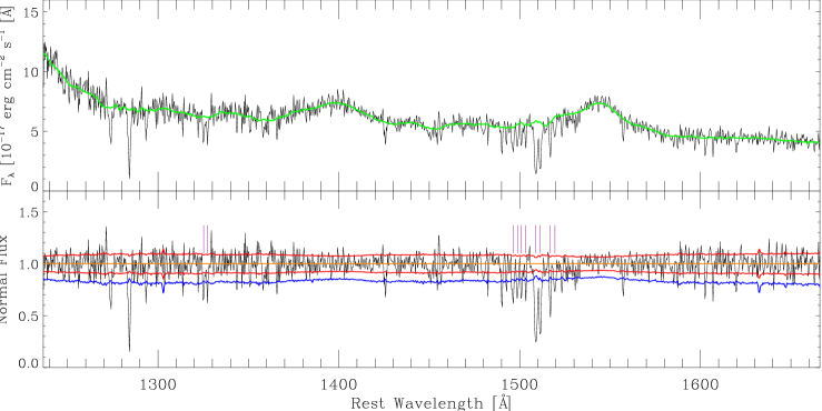
Figure 2: Spectrum of quasar SDSS J081617.02+163640.3. Upper panel: the pseudo-continuum fitting (green) is overplotted on the quasar spectrum. Lower panel: the quasar spectrum divided by the pseudo-continuum fitting (normalized spectrum). The red and blue lines are the $\rm\pm 1\sigma$ and $\rm-2\sigma$ flux uncertainty levels normalized by the pseudo-continuum fitting, respectively. The detected C iv  NALs with $S.L.\geq 2$ and $W_{r}\geq 0.2$ Å are marked with purple lines.

From 37,241 quasar spectra, we have detected a total number of 41,479 C iv  NALs with $1.4544\leq$$z_{\rm abs}$$\leq 4.9224$, of which 23,336 doublets with $z_{\rm abs}$$\rm\ll$$z_{\rm em}$ are released in Papers I and II, and 18,143 doublets with $z_{\rm abs}$$\rm\approx$$z_{\rm em}$ are newly detected in this paper. We distribute $z_{\rm abs}$ of these 41,479 C iv  NALs with back solid line in Figure 1, and list the properties of each absorption line in Table 1. Here after, all analyses about C iv  NALs are referred to the whole C iv  NAL sample that includes doublets released in Papers I and II, and newly detected in this paper.

Table 1: Catalog of C iv narrow absorption line systems

SDSS NAME	PLATEID	MJD	FIBERID	$\rm z_{em}$	$\rm z_{abs}$	$\rm W_{r}^{\lambda 1548}$	$\rm\sigma_{W_{r}}^{\lambda 1548}$	$\rm W_{r}^{\lambda 1551}$	$\rm\sigma_{W_{r}}^{\lambda 1551}$	$\rm S.L.^{\lambda 1548}$	$\rm S.L.^{\lambda 1551}$	$\rm\beta$
						Å	Å	Å	Å
000001.93-001427.4	4216	55477	0312	2.1645	2.1625	0.31	0.08	0.24	0.05	3.87	4.19	0.00063
000001.93-001427.4	4216	55477	0312	2.1645	2.1455	1.41	0.09	0.94	0.06	14.16	14.37	0.00602
000003.17+011510.6	4296	55499	0364	2.3543	1.8863	0.29	0.10	0.36	0.14	2.74	2.50	0.14915
000014.07+012951.5	4296	55499	0370	3.2284	2.6728	0.70	0.16	0.68	0.17	4.23	3.77	0.13994
000015.17+004833.2	4216	55477	0718	3.0277	2.5222	1.11	0.16	0.84	0.11	6.39	7.10	0.13331
000015.17+004833.2	4216	55477	0718	3.0277	2.9869	0.27	0.10	0.26	0.10	2.67	2.50	0.01018
000017.97+002426.9	4216	55477	0724	2.2825	2.2648	1.83	0.14	1.39	0.12	12.68	10.63	0.00541
000018.18+050803.6	4277	55506	0862	2.2278	2.1529	1.12	0.18	0.77	0.25	5.75	2.96	0.02347
000018.64+033254.1	4277	55506	0106	2.2375	2.2323	0.46	0.10	0.43	0.15	4.47	2.79	0.00161
000027.01+030715.5	4296	55499	0630	2.3533	1.9833	0.22	0.05	0.22	0.05	3.87	4.36	0.11639
000027.01+030715.5	4296	55499	0630	2.3533	2.1303	0.91	0.04	0.69	0.04	20.34	18.25	0.06871

Note: $\rm\beta=v/c=((1+z_{em})^{2}-(1+z_{abs})^{2})/((1+z_{em})^{2}+(1+z_{abs})^{2})$.

3 Completeness and redshift path

We run Monte Carlo simulation to test the efficiency of detection rate of absorbers with different signal-to-noise ratio. Using the spectral data of the BOSS quasar, we simulate 1000 C iv  NALs with different $S.L.$. Then, based on the spectral resolution of the BOSS, we randomly insert simulated C iv  doublets onto 400 quasar spectra, where the detected C iv  systems have been marked out, in the surveyed spectral region of C iv  NALs. Using the method and criteria described in Section 2, we collect the simulated doublets from the 400 quasar spectra. At a given $S.L.$, we define the completeness of detection as the ratio of the number of detected doublets to that of simulated doublets. The result is plotted in Figure 3, which suggests that the detectability tends to be complete in range of $S/N^{\lambda 1548}>4$.

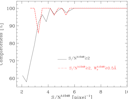
Figure 3: Completeness as a function of $S/N^{\lambda 1548}$. The black line accounts for the systems with $S/N^{\lambda 1548}\geq 2$, and the red dash line only considers the systems with $S/N^{\lambda 1548}\geq 2$ and $W_{\rm r}$$\geq 0.5$Å. The detection tends to be complete when $S/N^{\lambda 1548}\geq 4$.

In surveyed spectral region, the total redshift path covered by surveys as a function of signal-to-noise ratio per pixel ($S/N^{\rm\lambda 1548}$) under the pseudo-continuum fittings is derived by

$$\Delta Z(S/N^{\lambda 1548})=\sum_{i=1}^{N_{spec}}\int_{z_{i}^{min}}^{z_{i}^{max}}g_{i}(S/N^{\lambda 1548},z)dz,$$ (3)

where, the sum is over all quasar spectra used to survey absorption lines, the integral boundaries ([$z_{i}^{\rm min}$,$z_{i}^{\rm max}$]) are constrained by surveyed spectral region, the sensitivity function $g_{i}(S/N^{\rm\lambda 1548},z)=1$ if detection threshold $\rm S/N^{lim}~{}\leq S/N^{\rm\lambda 1548}$, otherwise $\rm g_{i}(S/N^{\rm\lambda 1548},z)=0$. In the left panel of Figure 4, we display the cumulative redshift path as a function of $S/N^{\rm\lambda 1548}$. The right panel of Figure 4 shows the total redshift path as a function of redshift. The pinnacles at $\rm z\approx 2.6$ and 2.8, and the obvious features at $\rm z>4.2$ are likely due to poor subtractions of sky lines, for example, [O i] and $\rm Na~{}D$, and $\rm OH$ lines.

Figure 4: Left panel: cumulative redshift path versus $S/N^{\rm\lambda 1548}$. Right panel: total redshift path versus redshift. The pinnacles at $\rm z\approx 2.6$ and 2.8, and the obvious features at $\rm z>4.2$ are likely due to poor subtractions of sky lines of [O i] and $\rm Na~{}D$, and $\rm OH$ lines in the SDSS spectra.

The spectral regions with strong emission lines often have higher signal-to-noise ratio than those without. Thus, for our identification procedure, the detection rate of C iv  doublet per redshift path could be higher for systems with $z_{\rm abs}$$\rm\approx$$z_{\rm em}$, which are located on or near to C iv  emission lines, than those with $z_{\rm abs}$$\rm\ll$$z_{\rm em}$. This should be noted in the following statistics and discussion.

4 Equivalent width distribution and saturability

The equivalent width of absorption line is an important parameter to reflect absorption strength and elemental abundance of absorber. In our C iv  NAL catalog, about 72% of absorbers have $W_{\rm r}^{\rm\lambda 1548}\geq 0.5$Å, $\sim$29% have $W_{\rm r}^{\rm\lambda 1548}\geq 1$Å, and $\sim$5% have $W_{\rm r}^{\rm\lambda 1548}\geq 2$Å. Using the SDSS quasar spectra, Cooksey et al. (2013) have assembled a catalog of intervening C iv  NALs with $\upsilon\equiv\beta c>5000$ $\rm km\,s^{-1}$. In order to compare our detection to that of Cooksey et al. (2013), we also use the criterion of $\upsilon\equiv\beta c=5000$ $\rm km\,s^{-1}$ to divide our C iv  NAL catalog into two subcatalogs of associated and intervening C iv  NALs. Figure 5 shows the distributions of the $W_{\rm r}$, which is clear that the absorptions of associated systems tend to be stronger than those of intervening ones (the black solid and dash lines). Figure 5 also indicates that the $W_{\rm r}$ distribution of intervening systems included in our catalog is similar to that of Cooksey et al. (2013) (the red and black solid lines). These distributions show a break around $W_{\rm r}^{\rm\lambda 1548}=0.5$Å, which might suggest an uncomplete detection for systems with $W_{\rm r}^{\rm\lambda 1548}<0.5$Å. The weak systems often have small $S.L.$, and the uncomplete detection suggested by the black solid line of Figure 3 might be mainly introduced by systems with $W_{\rm r}^{\rm\lambda 1548}<0.5$Å. When the Monte Carlo simulation for estimating the detected completeness (see Section 3) is limited to systems with $W_{\rm r}^{\rm\lambda 1548}\geq 0.5$Å, we show the detected completeness as a function of $S/N^{\rm\lambda 1548}$ with red dash line in Figure 3, which implies that the limit of $W_{\rm r}^{\rm\lambda 1548}\geq 0.5$Å does not change the cut, namely $S/N^{\rm\lambda 1548}>4$, of the detected completeness.

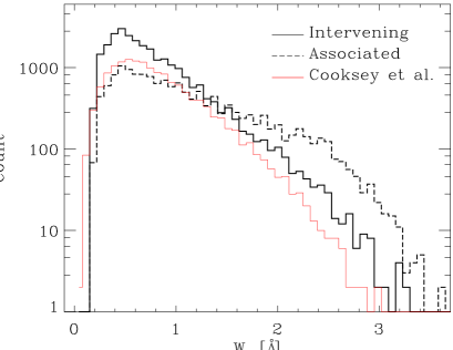
Figure 5: $W_{\rm r}$ distributions of C iv  NALs. The thick black solid line represents C iv  NALs with $\upsilon\equiv\beta c>5000$ $\rm km\,s^{-1}$ (intervening) included in our catalog, the dash line represents those with $\upsilon\equiv\beta c\leq 5000$ $\rm km\,s^{-1}$ (associated) included in our catalog, and the thin red solid line represents C iv  NALs of Cooksey et al. (2013). A break near 0.5Åis obvious.

The saturability of resonant absorption doublet can be obtained by the ratio of absorption strength ($\rm DR$, Strömgren, 1948). For C iv  resonant doublet, on the theoretical hand, $\rm DR\equiv W_{r}^{\rm\lambda 1548}/W_{r}^{\rm\lambda 1551}$ can vary from $1$ for full saturation to $2$ for full unsaturation. The error of the $\rm DR$ can be evaluated via

$$\sigma_{\rm DR}\equiv\Delta{\rm DR}=\sqrt{(\frac{\Delta W_{r}^{\rm\lambda 1548}}{W_{r}^{\rm\lambda 1551}})^{2}+(\frac{W_{r}^{\rm\lambda 1548}\Delta W_{r}^{\rm\lambda 1551}}{(W_{r}^{\rm\lambda 1551})^{2}})^{2}}$$ (4)

Figure 6 displays $W_{\rm r}^{\rm\lambda 1551}$ vs $W_{\rm r}^{\rm\lambda 1548}$. We find that about 73% of C iv  NALs fall into the range of $1\leq{\rm DR}\leq 2$, and only $\sim$ 7.7% of C iv  NALs are beyond the range of $1-\sigma_{\rm DR}\leq{\rm DR}\leq 2+\sigma_{\rm DR}$. Meanwhile, at $W_{\rm r}^{\rm\lambda 1548}>1$Å, the $\rm DR$ monotonically declines with increasing $W_{\rm r}^{\rm\lambda 1548}$, indicating that the stronger absorptions correspond to the more saturated absorptions that follows the curve of growth.

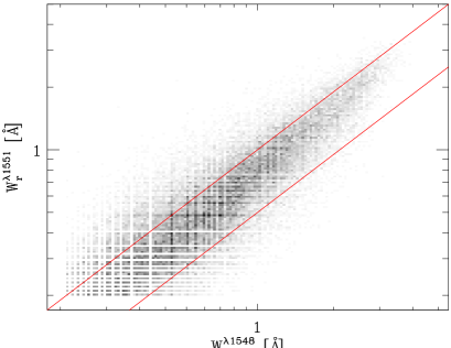
Figure 6: Local data point densities with grayscale. The red lines represent ${\rm DR}=W_{r}^{\rm\lambda 1548}/W_{r}^{\rm\lambda 1551}=1$ and 2, which correspond the theoretical limits of full saturation and unsaturation, respectively.

5 Discussion

5.1 The redshift density evolution of absorbers

Systematical survey of NALs on spectra of large quasar sample is in favor of studies of the absorber evolution and the connection between absorbers and galaxies. The redshift density is the count of absorbers with specified limits and normalized by redshift path length. In a specified redshift range, the redshift density of absorbers with a specified interval of $S/N^{\rm\lambda 1548}$ is derived via

$$\frac{\partial N}{\partial z}=\sum_{i}^{N_{\rm abs}}\frac{1}{\Delta Z(S/N^{\rm\lambda 1548}_{i})}$$ (5)

where $\Delta Z(S/N^{\rm\lambda 1548})$ is calculated by Equation 3, and the sum is over all C iv  NALs. Here, we only propagate the uncertainty of $\Delta Z(S/N^{\rm\lambda 1548})$ into the uncertainty of $\partial N/\partial z$. Using the spectral flux uncertainty limited by the SDSS, we invoke the Monte Carlo simulation to resample the spectral flux, and then limit the uncertainty of $\Delta Z(S/N^{\rm\lambda 1548})$ from Poisson statistics. Thus, the uncertainty of $\partial N/\partial z$ can be simply propagated by

$$\Delta(\partial N/\partial z)=\frac{N_{\rm abs}\times\Delta(\Delta Z(S/N^{\rm\lambda 1548}))}{\Delta Z(S/N^{\rm\lambda 1548})^{2}}$$ (6)

In several redshift ranges and at $S/N^{\rm\lambda 1548}\geq 2$, Table 2 lists the counts of C iv  NALs, $\Delta Z(S/N^{\rm\lambda 1548})$, and $\partial N/\partial z$, and Figure 7 displays the distribution of $\partial N/\partial z$ as a function of redshift with red filled circles. We also show the $\partial N/\partial z$ of Cooksey et al. (2013) with green filled triangles in Figure 7, which are measured from quasar spectra of the SDSS-I/II. It is clear that the $\partial N/\partial z$ of ours and Cooksey et al. (2013) have parallel evolution profile. The specified values of $\partial N/\partial z$ depend on methodologies used to determine redshift path. Thus $\partial N/\partial z$ related to $\Delta Z(S.L.)$ cannot be compared directly to $\partial N/\partial z$ related to $\Delta Z(W_{\rm r}^{\rm\lambda})$. The redshift path of this work is limited by $S.L.$, while that of Cooksey et al. (2013) is constrained by $W_{\rm r}^{\rm\lambda}$. Therefore, for comparison, the $\partial N/\partial z$ of Cooksey et al. (2013) plotted in Figure 7 has been scaled arbitrarily.

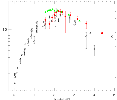
Figure 7: The reshift density evolution of absorbers from two surveys: this work (C iv  NALs, red filled circles), Cooksey et al. (2013)(C iv  NALs, green filled triangles). The star formation rate densities ($\dot{\rho}_{\ast}$) based on the data from Madau & Dickinson (2014) are displayed with black unfilled diamonds. The mappings between the left-axes of the triangles and the circles, and between the left and right y-axes are arbitrary.

Table 2: The redshift number density with $S/N^{\rm\lambda 1548}\geq 2$

z bin	$N_{\rm abs}$	$\rm\Delta Z$	$\rm\partial N/\partial z$
$[1.4544,1.6544)$	1123	65.8 ${}^{+15.5}_{-10.8}$	17.069${}^{+2.804}_{-4.009}$
$[1.6544,1.8544)$	2797	206.2${}^{+46.9}_{-34.9}$	13.569${}^{+2.299}_{-3.092}$
$[1.8544,1.9544)$	2786	142.7${}^{+29.3}_{-22.3}$	19.530${}^{+3.058}_{-4.005}$
$[1.9544,2.0544)$	3604	158.1${}^{+31.4}_{-24.1}$	22.801${}^{+3.479}_{-4.532}$
$[2.0544,2.1544)$	4423	168.5${}^{+30.7}_{-23.6}$	26.249${}^{+3.683}_{-4.783}$
$[2.1544,2.2544)$	5444	193.8${}^{+31.2}_{-23.9}$	28.093${}^{+3.465}_{-4.519}$
$[2.2544,2.3544)$	4902	178.4${}^{+28.5}_{-21.6}$	27.484${}^{+3.330}_{-4.392}$
$[2.3544,2.4544)$	4142	152.4${}^{+23.1}_{-17.4}$	27.176${}^{+3.113}_{-4.111}$
$[2.4544,2.6544)$	4897	237.4${}^{+145.1}_{-90.6}$	20.634${}^{+7.880}_{-12.614}$
$[2.6544,2.9544)$	3817	171.5${}^{+41.5}_{-29.7}$	22.256${}^{+3.861}_{-5.381}$
$[2.9544,3.3544)$	2465	136.4${}^{+27.9}_{-20.6}$	18.070${}^{+2.735}_{-3.691}$
$[3.3544,3.8544)$	866	62.9 ${}^{+15.2}_{-11.0}$	13.780${}^{+2.415}_{-3.325}$
$[3.8544,4.9224]$	212	26.4 ${}^{+15.7}_{-9.8}$	8.032${}^{+2.996}_{-4.778}$

Note — $N_{\rm abs}$ represents the number of detected C iv  NALs in corresponding redshift intervals.

The connection between the metal absorptions and the star formation rate densities has been widely explored in many previous works (e.g., Gauthier & Chen, 2011; Ménard et al., 2011; Zhu & Ménard, 2013; Huang et al., 2016). The cosmic star formation history peaks at $z\approx 2$ and decreases by about one magnitude from $z\sim 1$ to $z\sim 0$ (see recent review Madau & Dickinson, 2014). In order to establish the connection between $\partial N/\partial z$ and cosmic star formation histories, we scale the star formation rate densities ($\dot{\rho}=dM_{\ast}/(dtdAdX)$) with $dX/dz$, where X is the comoving distance and A is the comoving area. The scaling $\dot{\rho}$ is plotted with open diamonds in Figure 7. The global evolution shapes of $\dot{\rho}dX/dz$ and $\partial N/\partial z$ are very similar.

The redshift number density $\partial N/\partial z$ relates to the volume density of absorbers $n_{\rm vol}$ and their physical cross-section $\sigma_{\rm phys}$. Therefore, the evolution of $\partial N/\partial z$ is possibly dominated by the product of $n_{\rm vol}\sigma_{\rm phys}$. C iv  metal absorbing gas relates to galaxy (e.g., Chen, Lanzetta, & Webb, 2001; Adelberger et al., 2005; Tinker & Chen, 2008; Martin et al., 2010; Burchett et al., 2013; Bordoloi et al., 2014). Both the number of galaxies and their surrounding gas (halo) likely evolve over cosmic time, so evolutions in both $n_{\rm vol}$ and $\sigma_{\rm phys}$ can change the value of $\partial N/\partial z$:

$$\frac{\partial N}{\partial z}\propto n_{\rm vol}(z)\sigma_{\rm phys}(z).$$ (7)

Using the UV luminosity functions from Bouwens et al. (2007), Reddy & Steidel (2009) and Oesch et al. (2010), Cooksey et al. (2013) derived the UV-selected galaxy volume density ($n_{\rm vol}$) by integrating the best fitting Schechter function, which increase by a factor of 2 to 3 in redshift range of 5 to 1.5 (see Figure 12 of Cooksey et al. (2013)). In similar redshift range, Figure 7 and Table 2 show that the $\partial N/\partial z$ increases by a factor of 3 to 4. In this case, the physical cross-section $\sigma_{\rm phys}$ of absorbing cloud could modestly increase over cosmic time. This increase might be from a comprehensive evolution of absorber’s UV ionizing background, metallicity, and geometric size.

5.2 The quasar-frame velocity distribution

NALs are mainly arisen from: (1) material of intervening galaxies lying on quasar sightlines; and (2) material associated with quasar themselves, which can be related to quasars’ host galaxies, winds/outflows and surrounding environment. The former produces intervening NALs with $z_{\rm abs}$$\ll$$z_{\rm em}$, and the latter brings about associated NALs with $z_{\rm abs}$$\approx$$z_{\rm em}$. Associated NALs are alluring since they provide a powerful tool to explore AGN feedback. BALs are unambiguously associated with quasars. However, it is difficult to identify whether one NAL is related to quasar or not. The line variability and partial coverage analysis are frequently applied to diagnose the associated NALs. Only small sample of variable NALs are detected up to nowadays (e.g., Narayanan et al., 2004; Wise et al., 2004; Hacker et al., 2013; Chen et al., 2015). Therefore, the statistics is often utilized to decompose associated population from a large NAL catalog (e.g., Misawa et al., 2007; Nestor, Hamann, & Rodriguez Hidalgo, 2008; Wild et al., 2008).

If NALs are associated to quasars, then the differences between $z_{\rm abs}$ and $z_{\rm em}$ should be dominated by motions of absorbers relative to quasars, and the relative velocities can be derived by

$$\beta\equiv\frac{\upsilon}{c}=\frac{(1+z_{\rm em})^{2}-(1+z_{\rm abs})^{2}}{(1+z_{\rm em})^{2}+(1+z_{\rm abs})^{2}}.$$ (8)

We note that $z_{\rm abs}$ determined from NALs have high accuracy, while $z_{\rm em}$ measured from broad emission lines can show an uncertainty from 100 $\rm km\,s^{-1}$ to 3000 $\rm km\,s^{-1}$ (e.g., Hewett & Wild, 2010; Shen et al., 2011; Shen, 2016). Using the near-infrared quasar spectra, Shen (2016) revealed that, after accounting for measurement errors, redshifts estimated from broad Mg ii$\lambda$2798 emission lines have an intrinsical uncertainty of about 200 $\rm km\,s^{-1}$ with respect to the redshifts determined by [O iii]$\lambda$5007 emission lines. This small uncertainty implies that Mg ii emission line is a better indicator to estimate quasar systemic redshift relative to C iii], C iv , and Ly $\alpha$  emission lines (e.g., Hewett & Wild, 2010; Shen et al., 2011).

Chen, Gu, & Chen (2015) has systematically surveyed Mg ii NALs on 43,260 BOSS quasar spectra of the DR9Q from redward of Ly $\alpha$  to red wing of Mg ii$\lambda$2798 emission lines, which results in a total number of 18,598 Mg ii doublets with $0.2933\leq$$z_{\rm abs}$$\leq 2.6529$. The method used in Chen, Gu, & Chen (2015) to search for NALs is exactly the same as this work. In order to compare the $\beta$ distribution of C iv  NALs to that of Mg ii NALs, we make use of the Mg ii NALs included in Chen, Gu, & Chen (2015). We limit C iv  NALs to quasars with $z_{\rm em}$$\leq 2.2$ so that Mg ii$\lambda$2798 emission lines can be available by the BOSS spectra. Surveyed spectral region of C iv  NALs is between Ly $\alpha$  and C iv$\lambda$1549 emission lines, which constrains $\beta<0.16$ for C iv  NALs. And that of Mg ii NALs is between Ly $\alpha$  and Mg ii$\lambda$2798 emission lines, which permits measurement of much higher $\beta$ values for Mg ii NALs. In order to make a consistent comparison, we limit both C iv  and Mg ii NALs with $\beta<0.15$. Taking into account of $z_{\rm em}$$\leq 2.2$ and $\beta<0.15$, there are 5922 C iv  NALs and 3012 Mg ii NALs. We display the $\beta$ distributions of both C iv  and Mg ii NALs in Figure 8.

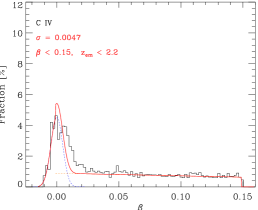
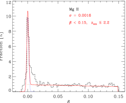
Figure 8: Relative velocity distributions of absorbers with $\beta<0.15$ and $z_{\rm em}\leq 2.2$. The y-axes are the counts of absorbers normalized by the total numbers of absorbers contained in corresponding subsamples. The red curves are the reduced $\rm\chi^{2}$ fittings of a combination of a Gaussian function centred at $\beta=0$ and a linear function using the data with $\beta<0$ and $>0.06$. The blue and orange dash lines are the Gaussian and linear components, respectively. Left panel: the KS test suggests a probability of $P<10^{\rm-6}$ that the two populations draw from the same parent sample. Middle panel: C iv  absorbers with $\sigma=0.0047$ for the Gaussian component. Right panel: Mg ii absorbers with $\sigma=0.0016$ for the Gaussian component.

In the calculation of $\beta$, we have made an assumption that all NALs are produced by quasar self-absorptions. In fact, the catalogs contain absorptions from (1) the first population: cosmologically intervening galaxies; (2) the second population: quasar host galaxies or galaxy clusters/groups that quasars reside in, which is often called as environmental absorptions; and (3) the third population: quasar outflows. Although ultra-fast outflows have been detected by many researchers (e.g., Hamann et al., 2011; Tombesi et al., 2011; Chen & Qin, 2013; Gupta et al., 2013), the vast majority of absorbers with a large $\beta$ belong to the first population. When absorbers fall into the second population, some absorbers move toward the observer and some away, and the $\beta$ would show a normal distribution centred at $\beta=0$. In addition, galaxies around quasars are clustered/grouped, so one expects an excess of associated absorbers with respect to cosmologically intervening absorbers. Absorbers of the third population move towards the observer, thus they have $\beta>0$ and are expected to destroy the normal distribution of $\beta$ of the second population absorptions. Figure 8 clearly shows that there are an abnormal excess in range of $\beta<0.02$ and a flat tail in range of $\beta>0.02$. This suggests that the data in range of $\beta>0.02$ would be dominated by absorptions of the first population, and those in range of $\beta<0.02$ be mainly contributed from absorptions of the second and third populations.

In theory, quasar outflows do not affect the $\beta$ distribution of associated absorbers with $\beta<0$. In Figure 8, absorbers with $\beta>0.06$ are probably contributed from cosmologically intervening absorptions. We explore a combination of a Gaussian function accounting for environmental absorptions and a linear function accounting for intervening absorptions to fit the data with $\beta<0$ and $>0.06$. This results in Gaussian components with $\sigma=0.0047$ for C iv  NALs and $\sigma=0.0016$ for Mg ii NALs. The fitting results are plotted with color lines in Figure 8. It is clear that a combination of a Gaussian and a linear functions can not well characterize the overall distributions, and the excesses located at $\beta\approx 0.01$ are very remarkable with respect to fitting curves, which likely are the contribution of quasar outflows.

Since C iv  (64.49 eV) has much higher ionization potential than Mg ii (15.035 eV), we expect the associated C iv  and Mg ii NALs to show different statistical properties. Recalling Figure 8, in range of $\beta<0.02$, the $\beta$ distribution of Mg ii absorbers is more compact than the same values of C iv  absorbers. KS test derives a probability of $P<10^{\rm-6}$ that the $\beta$ of C iv  and Mg ii absorbers draw from the same parent sample. The multi-component fittings overplotted with red lines imply that the dispersion of C iv  environmental absorptions ($\sigma=0.0047$) is much larger than the same value of Mg ii environmental absorptions ($\sigma=0.0016$). In addition, with respect to multi-component fittings, the excessive tail of Mg ii absorbers reaches a value of $\beta\approx 0.02$, but that of C iv  absorbers can extend out to a higher value of $\beta>0.04$. This suggests that the higher ionization outflows have the larger maximum velocity.

Using C iv  and Mg ii NALs detected from quasar spectra of the SDSS DR3, the model of Wild et al. (2008) predicts that the scales that the quasar photoevaporates environmental absorbers are related to ionization energies of ions. The radius of 300 kpc for survived C iv  absorbers is much smaller than that of 800 kpc for survived Mg ii absorbers. This discrepancy is also clearly reflected by our multi-component fittings (see Figure 8): $\sigma=0.0047$ for C iv  absorbers, and $\sigma=0.0016$ for Mg ii ones.

Using the emission redshifts of the SDSS pipeline, Nestor, Hamann, & Rodriguez Hidalgo (2008) obtained a dispersion with a value of 913 $\rm km\,s^{-1}$ for C iv  environmental absorbers after deconvolving the redshift uncertainty. When based on redshifts determined by Mg ii emission lines, they found a value of about 450 $\rm km\,s^{-1}$. For our multi-component fitting, we obtain a dispersion with a value of 728 $\rm km\,s^{-1}$, which is slightly larger than that of 450 $\rm km\,s^{-1}$. Our limit of $z_{\rm em}$$\leq 2.2$ can reduce, on a certain extent, the uncertainties of emission redshifts. However, we can not guarantee that the significant Mg ii emission line was imprinted on each quasar spectrum. Thus, the uncertainties of emission redshifts could be larger than those determined by Mg ii emission lines.

5.3 Dependence on the radio detection

The observational area of the Faint Images of the Radio Sky at Twenty centimeter survey (FIRST, Becker, White, & Helfand, 1995) coincides with that of the SDSS. Over most of the area, the FIRST survey is limited to a detection threshold of 1 $\rm mJy$. In order to investigate the dependence of associated absorber properties on radio detection, we match our parent quasar sample with the FIRST within a radius of $30^{\prime\prime}$. Figure 8 shows that some outflow absorbers can reach a high velocity. Here, we loosely constrain associated absorbers with $\beta<0.03$. Combining the limits of $\beta<0.03$ and $z_{\rm em}$$\leq 2.2$, there are 2741 and 198 C iv  NALs imprinted on the spectra of FIRST undetected and detected quasars, respectively. In terms of the luminosity at 20 $\rm cm$, the quasar with a luminosity $>10^{\rm 25}~{}\rm W/Hz$ is defined as radio-loud one, inversely radio-quiet one. According to this definition, the FIRST detected quasars of the 198 C iv  absorbers belong to radio-loud population. Because the small sample of the FIRST detected quasars, we do not discuss the dependence of associated absorber properties on radio morphologies.

We display $\beta$ distributions in Figure 9. No significant difference is shown between the $\beta$ of the FIRST detected and undetected NALs. This similar result is also exhibited in the $W_{\rm r}$ distributions (see Figure 10). The $\beta$ distributions do not coincide with those of Wild et al. (2008), who found that the $\beta$ measured from radio-loud quasar spectra are more compact at $\beta\approx 0$ than the same values measured from radio-quiet ones. There are only 69 FIRST detected quasars satisfied our criteria. This number is too small to allow us to further investigate the different $\beta$ distributions between our results and Wild et al. (2008).

Figure 9: Relative velocity distributions of absorbers with $\beta<0.03$ and $z_{\rm em}$$\leq 2.2$. The y-axis are the counts of absorbers normalized by the total numbers of absorbers contained in corresponding subsamples. The solid (dash) lines represent the quasars without (with) the FIRST detection. KS test yields a $P=0.03$

Figure 10: $W_{\rm r}$ distributions of absorbers with $\beta<0.03$ and $z_{\rm em}$$\leq 2.2$. The y-axis are the counts of absorbers normalized by the total numbers of absorbers contained in corresponding subsamples. The solid (dash) lines represent the quasars without (with) the FIRST detection. KS test yields a $P=0.7$

5.4 Dependence on the UV continuum luminosity

The ionizing radiation from quasars produces feedback to surrounding gas, which can affect gaseous ionization state, density and kinematics. The dependence of this feedback on the quasar luminosity can be studied by absorbers surrounding quasars (e.g., Pan & Chen, 2013; Johnson, Chen, & Mulchaey, 2015). We exclude quasars that the flux data at 1350Å are not available by the BOSS spectra due to quasar redshifts and that are located at $z_{\rm em}$$>2.2$, and limit absorbers with $\beta<0.03$. This results in a sample of 2866 C iv  NALs. We divide the resulting sample at median value of the continuum luminosity at rest frame 1350Å ($L_{\rm 1350}=10^{\rm 44.63}$ ${\rm erg\,s^{-1}}$) into low- and high-luminosity quasar samples, where continuum luminosities are measured from pseudo-continuum fitting.

The $\beta$ and $W_{\rm r}$ distributions of both low- and high-luminosity quasar samples are shown in Figures 11 and 12, respectively. KS test yields a $P<10^{\rm-16}$ for the $\beta$ and a $P<10^{\rm-13}$ for the $W_{\rm r}$, which suggests that the ionizing radiation of quasars acts on both $\beta$ and $W_{\rm r}$ distributions. We also note that the low-luminosity quasars have stronger absorption strengths.

Figure 11: Relative velocity distributions of absorbers with $\beta<0.03$ and $z_{\rm em}$$\leq 2.2$. The y-axis are the counts of absorbers normalized by the total numbers of absorbers contained in corresponding subsamples. The solid (dash) lines represent quasars with continuum luminosities less (greater) than corresponding median values. KS test yields a $P<10^{\rm-16}$.

Figure 12: $W_{\rm r}$ distributions of absorbers with $\beta<0.03$ and $z_{\rm em}$$\leq 2.2$. The y-axis are the counts of absorbers normalized by the total numbers of absorbers contained in corresponding subsamples. KS test yields a $P<10^{\rm-10}$.

The SDSS quasars are obtained by flux limited surveys, and consequently the high luminosity quasars can be obtained at high redshifts. Therefore, the differences of $\beta$ and $W_{\rm r}$ distributions between low- and high-luminosity quasars might be the evolution result of quasar surrounding gas. We find that both low- and high-luminosity quasars have similar median $z_{\rm em}$. Thus, the differences reflected by Figures 11 and 12 are not originated in the evolution of quasar surrounding gas.

It is interesting that the high-luminosity quasars tend to show larger velocity ($\beta$) C iv  NALs with smaller absorption strengths, which might be related to the radiative acceleration by quasar luminosity and ionization condition of CGMs around quasars. For high-luminosity quasars, the enormous power of outflows and the energetic radiation from accretion disc could produce stronger feedback to surrounding gas of quasars. In this case, surrounding gas of high-luminosity quasars is possibly accelerated to higher velocity and photo-ionized to higher level.

6 Summary

Using the BOSS quasar spectra (DR9Q), combining the two early works (Papers I and II), we have detected a total number of 41,479 C iv  NALs with $1.4544\leq$$z_{\rm abs}$$\leq 4.9224$ in wavelength range between Ly $\alpha$  and C iv$\lambda$1549 emission lines. The detectability tend to be complete when $S/N^{\rm\lambda 1548}>4$. Ours main results are as follows.

1. 92.3% of C iv  NALs fall into the range of $1-\sigma_{DR}\leq DR\leq 2+\sigma_{DR}$, and tend to be the more saturated absorptions with the stronger absorptions that follows the curve of growth. The associated systems show significant absorptions when compared to the intervening ones.

2. The redshift density evolution shape of C iv  absorbers is similar to the history of the cosmic star formation, which indicates that C iv  absorbers may be connected to the star formation activities within galaxies. Thus, absorption lines imprinted on the spectra of background objects are possibly a powerful tool to investigate faint and even invisible galaxies.

3. Comparing $\beta$ distributions of C iv  and Mg ii absorbers, we find clear distinctions. The $\beta$ of C iv  absorbers are more compact to $\beta\approx 0$, and have longer extended tail. In addition, the dispersion of C iv  environmental absorptions is much larger than that of Mg ii environmental absorptions. The C iv  has an ionization energy of 64.49 $\rm eV$, which is obviously different from that of 15.035 $\rm eV$ of the Mg ii. The clearly different ionization energies of C iv  and Mg ii may play an important role to the distinct $\beta$ properties between the two kinds of absorbers.

4. For associated C iv  absorbers ($\beta<0.03$), when compared with the low-luminosity quasars, high-luminosity quasars tend to have larger $\beta$ and weaker absorptions.

The line number density of absorbers depends not only on their volume density, but on physical cross-section and ionizing background of absorbing clouds. One of our future works will investigate the properties of absorbers that intersect both sightlines of a quasar pair (two close quasars on sky). This might provide a useful limit to the geometric cross-section of absorbing cloud. Deep imaging/spectroscopy observations to this kind of absorbers might also provide useful information about absorption line formation by comparing absorption strength and profile of absorption lines and characteristics of galaxy halo, such as gas distribution, star formation rate, orientations of disc and outflow, and so on.

The properties of CGMs and outflows of quasars are crucial to comprehend the quasar feedback and evolution of host galaxy. Time variability and partial coverage analysis is two efficient ways to identify absorption lines of quasar outflow and environment. Therefore, high resolution observations of the quasars with variable absorption line could provide well opportunity to investigate the properties of quasar outflow and CGM.

The authors are very grateful to the anonymous referee for his/her critical comments and instructive suggestions, which significantly strengthened the analyses in this work. This work was supported by the National Natural Science Foundation of China (NO. 11363001, grants 11273015, 11573013 and 11133001), National Basic Research Program (973 program No. 2013CB834905), the Guangxi Natural Science Foundation (2015GXNSFBA139004), and the Guangxi University of Science and Technology research projects (No. KY2015YB289). Y.M.C. acknowledges support from the Opening Project of Key Laboratory of Computational Astrophysics, National Astronomical Observatories, Chinese Academy of Sciences.

Funding for SDSS-III has been provided by the Alfred P. Sloan Foundation, the Participating Institutions, the National Science Foundation, and the U.S. Department of Energy Office of Science. The SDSS-III web site is http://www.sdss3.org/.

SDSS-III is managed by the Astrophysical Research Consortium for the Participating Institutions of the SDSS-III Collaboration including the University of Arizona, the Brazilian Participation Group, Brookhaven National Laboratory, Carnegie Mellon University, University of Florida, the French Participation Group, the German Participation Group, Harvard University, the Instituto de Astrofisica de Canarias, the Michigan State/Notre Dame/JINA Participation Group, Johns Hopkins University, Lawrence Berkeley National Laboratory, Max Planck Institute for Astrophysics, Max Planck Institute for Extraterrestrial Physics, New Mexico State University, New York University, Ohio State University, Pennsylvania State University, University of Portsmouth, Princeton University, the Spanish Participation Group, University of Tokyo, University of Utah, Vanderbilt University, University of Virginia, University of Washington, and Yale University.

References

- Abazajian et al. (2009) Abazajian K. N., et al., 2009, ApJS, 182, 543-558
- Adelberger et al. (2005) Adelberger K. L., Shapley A. E., Steidel C. C., Pettini M., Erb D. K., Reddy N. A., 2005, ApJ, 629, 636
- Balashev et al. (2014) Balashev S. A., Klimenko V. V., Ivanchik A. V., Varshalovich D. A., Petitjean P., Noterdaeme P., 2014, MNRAS, 440, 225
- Arrigoni Battaia et al. (2016) Arrigoni Battaia F., Hennawi J. F., Cantalupo S., Prochaska J. X., 2016, arXiv, arXiv:1604.02942
- Becker, White, & Helfand (1995) Becker R. H., White R. L., Helfand D. J., 1995, ApJ, 450, 559
- Bordoloi et al. (2014) Bordoloi R., et al., 2014, ApJ, 796, 136
- Borthakur et al. (2015) Borthakur S., et al., 2015, ApJ, 813, 46
- Bouché et al. (2013) Bouché N., Murphy M. T., Kacprzak G. G., Péroux C., Contini T., Martin C. L., Dessauges-Zavadsky M., 2013, Sci, 341, 50
- Bouwens et al. (2007) Bouwens R. J., Illingworth G. D., Franx M., Ford H., 2007, ApJ, 670, 928
- Burchett et al. (2013) Burchett J. N., Tripp T. M., Werk J. K., Howk J. C., Prochaska J. X., Ford A. B., Davé R., 2013, ApJ, 779, L17
- Cantalupo et al. (2014) Cantalupo S., Arrigoni-Battaia F., Prochaska J. X., Hennawi J. F., Madau P., 2014, Natur, 506, 63
- Cen & Chisari (2011) Cen R., Chisari N. E., 2011, ApJ, 731, 11
- Chen, Lanzetta, & Webb (2001) Chen H.-W., Lanzetta K. M., Webb J. K., 2001, ApJ, 556, 158
- Chen, Gu, & Chen (2015) Chen Z.-F., Gu Q.-S., Chen Y.-M., 2015, ApJS, 221, 32
- Chen et al. (2015) Chen Z.-F., Gu Q.-S., Chen Y.-M., Cao Y., 2015, MNRAS, 450, 3904
- Chen et al. (2013) Chen Z.-F., Li M.-S., Huang W.-R., Pan C.-J., Li Y.-B., 2013, MNRAS, 434, 3275
- Chen & Qin (2013) Chen Z.-F., Qin Y.-P., 2013, ApJ, 777, 56
- Chen et al. (2014a) Chen Z.-F., Qin Y.-P., Pan C.-J., Huang W.-R., Qin M., Wu H.-N., 2014a, ApJS, 210, 7 (PaperI)
- Chen et al. (2014b) Chen Z.-F., Qin Y.-P., Qin M., Pan C.-J., Pan D.-S., 2014b, ApJS, 215, 12 (PaperII)
- Chartas et al. (2012) Chartas G., Eracleous M., Misawa T., Giustini G., Charlton J., 2012, ASPC, 460, 37
- Chartas et al. (2009) Chartas G., et al., 2009, NewAR, 53, 128
- Dawson et al. (2013) Dawson K. S., et al., 2013, AJ, 145, 10
- Cooksey et al. (2013) Cooksey K. L., Kao M. M., Simcoe R. A., O’Meara J. M., Prochaska J. X., 2013, ApJ, 763, 37
- Cooksey et al. (2011) Cooksey K. L., Prochaska J. X., Thom C., Chen H.-W., 2011, ApJ, 729, 87
- Davé, Finlator, & Oppenheimer (2012) Davé R., Finlator K., Oppenheimer B. D., 2012, MNRAS, 421, 98
- Dekel et al. (2009) Dekel A., et al., 2009, Natur, 457, 451
- Eisenstein et al. (2001) Eisenstein D. J., et al., 2001, AJ, 122, 2267
- Eisenstein et al. (2011) Eisenstein D. J., et al., 2011, AJ, 142, 72
- Farina et al. (2014) Farina E. P., Falomo R., Scarpa R., Decarli R., Treves A., Kotilainen J. K., 2014, MNRAS, 441, 886
- Fechner & Richter (2009) Fechner C., Richter P., 2009, A&A, 496, 31
- Ford et al. (2014) Ford A. B., Davé R., Oppenheimer B. D., Katz N., Kollmeier J. A., Thompson R., Weinberg D. H., 2014, MNRAS, 444, 1260
- Fox et al. (2007) Fox A. J., Petitjean P., Ledoux C., Srianand R., 2007, A&A, 465, 171
- Fox et al. (2009) Fox A. J., Prochaska J. X., Ledoux C., Petitjean P., Wolfe A. M., Srianand R., 2009, A&A, 503, 731
- Gauthier & Chen (2011) Gauthier J.-R., Chen H.-W., 2011, MNRAS, 418, 2730
- Gupta et al. (2013) Gupta A., Mathur S., Krongold Y., Nicastro F., 2013, ApJ, 772, 66
- Gunn et al. (2006) Gunn J. E., et al., 2006, AJ, 131, 2332
- Hacker et al. (2013) Hacker T. L., Brunner R. J., Lundgren B. F., York D. G., 2013, MNRAS, 434, 163
- Hamann et al. (2011) Hamann F., Kanekar N., Prochaska J. X., Murphy M. T., Ellison S., Malec A. L., Milutinovic N., Ubachs W., 2011, MNRAS, 410, 1957
- Hennawi & Prochaska (2013) Hennawi J. F., Prochaska J. X., 2013, ApJ, 766, 58
- Hennawi et al. (2015) Hennawi J. F., Prochaska J. X., Cantalupo S., Arrigoni-Battaia F., 2015, Sci, 348, 779
- Hewett & Wild (2010) Hewett P. C., Wild V., 2010, MNRAS, 405, 2302
- Huang et al. (2016) Huang Y.-H., Chen H.-W., Johnson S. D., Weiner B. J., 2016, MNRAS, 455, 1713
- Husband et al. (2015) Husband K., Bremer M. N., Stanway E. R., Lehnert M. D., 2015, MNRAS, 452, 2388
- Johnson, Chen, & Mulchaey (2015) Johnson S. D., Chen H.-W., Mulchaey J. S., 2015, MNRAS, 452, 2553
- Kacprzak et al. (2011) Kacprzak G. G., Churchill C. W., Barton E. J., Cooke J., 2011, ApJ, 733, 105
- Kacprzak et al. (2007) Kacprzak G. G., Churchill C. W., Steidel C. C., Murphy M. T., Evans J. L., 2007, ApJ, 662, 909
- Kacprzak et al. (2015) Kacprzak G. G., Muzahid S., Churchill C. W., Nielsen N. M., Charlton J. C., 2015, ApJ, 815, 22
- Keeney et al. (2013) Keeney B. A., Stocke J. T., Rosenberg J. L., Danforth C. W., Ryan-Weber E. V., Shull J. M., Savage B. D., Green J. C., 2013, ApJ, 765, 27
- Kollmeier et al. (2006) Kollmeier J. A., Miralda-Escudé J., Cen R., Ostriker J. P., 2006, ApJ, 638, 52
- Lü, Qin, & Gupta (2007) Lü L.-Z., Qin Y.-P., Gupta A. C., 2007, ApJ, 669, 74
- Ménard et al. (2011) Ménard B., Wild V., Nestor D., Quider A., Zibetti S., Rao S., Turnshek D., 2011, MNRAS, 417, 801
- Madau & Dickinson (2014) Madau P., Dickinson M., 2014, ARA&A, 52, 415
- Martin et al. (2010) Martin C. L., Scannapieco E., Ellison S. L., Hennawi J. F., Djorgovski S. G., Fournier A. P., 2010, ApJ, 721, 174
- Martin et al. (2014) Martin D. C., Chang D., Matuszewski M., Morrissey P., Rahman S., Moore A., Steidel C. C., 2014, ApJ, 786, 106
- Martin et al. (2015) Martin D. C., Matuszewski M., Morrissey P., Neill J. D., Moore A., Cantalupo S., Prochaska J. X., Chang D., 2015, Natur, 524, 192
- Matejek & Simcoe (2012) Matejek M. S., Simcoe R. A., 2012, ApJ, 761, 112
- Misawa et al. (2007) Misawa T., Charlton J. C., Eracleous M., Ganguly R., Tytler D., Kirkman D., Suzuki N., Lubin D., 2007, ApJS, 171, 1
- Murga et al. (2015) Murga M., Zhu G., Ménard B., Lan T.-W., 2015, MNRAS, 452, 511
- Muzahid et al. (2015) Muzahid S., Kacprzak G. G., Churchill C. W., Charlton J. C., Nielsen N. M., Mathes N. L., Trujillo-Gomez S., 2015, ApJ, 811, 132
- Narayanan et al. (2004) Narayanan D., Hamann F., Barlow T., Burbidge E. M., Cohen R. D., Junkkarinen V., Lyons R., 2004, ApJ, 601, 715
- Nestor, Hamann, & Rodriguez Hidalgo (2008) Nestor D., Hamann F., Rodriguez Hidalgo P., 2008, MNRAS, 386, 2055
- Nestor, Turnshek, & Rao (2005) Nestor D. B., Turnshek D. A., Rao S. M., 2005, ApJ, 628, 637
- Nielsen et al. (2015) Nielsen N. M., Churchill C. W., Kacprzak G. G., Murphy M. T., Evans J. L., 2015, ApJ, 812, 83
- Oesch et al. (2010) Oesch P. A., et al., 2010, ApJ, 725, L150
- Pâris et al. (2012) Pâris I., et al., 2012, A&A, 548, A66
- Pan & Chen (2013) Pan C.-J., Chen Z.-F., 2013, JApA, 34, 357
- Pérez-Ràfols et al. (2015) Pérez-Ràfols I., Miralda-Escudé J., Lundgren B., Ge J., Petitjean P., Schneider D. P., York D. G., Weaver B. A., 2015, MNRAS, 447, 2784
- Qin et al. (2013) Qin Y.-P., et al., 2013, PASJ, 65, 8
- Quider et al. (2011) Quider A. M., Nestor D. B., Turnshek D. A., Rao S. M., Monier E. M., Weyant A. N., Busche J. R., 2011, AJ, 141, 137
- Reddy & Steidel (2009) Reddy N. A., Steidel C. C., 2009, ApJ, 692, 778
- Richter (2012) Richter P., 2012, ApJ, 750, 165
- Rubin et al. (2012) Rubin K. H. R., Prochaska J. X., Koo D. C., Phillips A. C., 2012, ApJ, 747, L26
- Savage et al. (2014) Savage B. D., Kim T.-S., Wakker B. P., Keeney B., Shull J. M., Stocke J. T., Green J. C., 2014, ApJS, 212, 8
- Seyffert et al. (2013) Seyffert E. N., Cooksey K. L., Simcoe R. A., O’Meara J. M., Kao M. M., Prochaska J. X., 2013, ApJ, 779, 161
- Shen (2016) Shen Y., 2016, ApJ, 817, 55
- Shen et al. (2011) Shen Y., et al., 2011, ApJS, 194, 45
- Shen & Ménard (2012) Shen Y., Ménard B., 2012, ApJ, 748, 131
- Smee et al. (2013) Smee S. A., et al., 2013, AJ, 146, 32
- Songaila (2005) Songaila A., 2005, AJ, 130, 1996
- Springel & Hernquist (2003) Springel V., Hernquist L., 2003, MNRAS, 339, 289
- Strömgren (1948) Strömgren B., 1948, ApJ, 108, 242
- Tinker & Chen (2008) Tinker J. L., Chen H.-W., 2008, ApJ, 679, 1218-1231
- Tombesi et al. (2011) Tombesi F., Cappi M., Reeves J. N., Palumbo G. G. C., Braito V., Dadina M., 2011, ApJ, 742, 44
- Tripp et al. (2011) Tripp T. M., et al., 2011, Sci, 334, 952
- Tripp et al. (2008) Tripp T. M., Sembach K. R., Bowen D. V., Savage B. D., Jenkins E. B., Lehner N., Richter P., 2008, ApJS, 177, 39-102
- Vanden Berk et al. (2008) Vanden Berk D., et al., 2008, ApJ, 679, 239-259
- Wild et al. (2008) Wild V., et al., 2008, MNRAS, 388, 227
- Wise et al. (2004) Wise J. H., Eracleous M., Charlton J. C., Ganguly R., 2004, ApJ, 613, 129
- York et al. (2000) York D. G., et al., 2000, AJ, 120, 1579
- Zhu & Ménard (2013) Zhu G., Ménard B., 2013, ApJ, 773, 16
- Zhu & Ménard (2013) Zhu G., Ménard B., 2013, ApJ, 770, 130