Computerized Tomography with Total Variation and with Shearlets

Abstract

To reduce the x-ray dose in computerized tomography (CT), many constrained optimization approaches have been proposed aiming at minimizing a regularizing function that measures lack of consistency with some prior knowledge about the object that is being imaged, subject to a (predetermined) level of consistency with the detected attenuation of x-rays. One commonly investigated regularizing function is total variation (TV), while other publications advocate the use of some type of multiscale geometric transform in the definition of the regularizing function, a particular recent choice for this is the shearlet transform. Proponents of the shearlet transform in the regularizing function claim that the reconstructions so obtained are better than those produced using TV for texture preservation (but may be worse for noise reduction). In this paper we report results related to this claim. In our reported experiments using simulated CT data collection of the head, reconstructions whose shearlet transform has a small $\ell_{1}$-norm are not more efficacious than reconstructions that have a small TV value. Our experiments for making such comparisons use the recently-developed superiorization methodology for both regularizing functions. Superiorization is an automated procedure for turning an iterative algorithm for producing images that satisfy a primary criterion (such as consistency with the observed measurements) into its superiorized version that will produce results that, according to the primary criterion are as good as those produced by the original algorithm, but in addition are superior to them according to a secondary (regularizing) criterion. The method presented for superiorization involving the $\ell_{1}$-norm of the shearlet transform is novel and is quite general: It can be used for any regularizing function that is defined as the $\ell_{1}$-norm of a transform specified by the application of a matrix. Because in the previous literature the split Bregman algorithm is used for similar purposes, a section is included comparing the results of the superiorization algorithm with the split Bregman algorithm.

Keywords: Computerized Tomography, Shearlet, TV, Reconstruction Algorithm, Optimization, Superiorization, Split Bregman, ART

1 Introduction

In a typical x-ray computerized tomography (CT) study, projections from various orientations are obtained by the scanner detectors and later processed to produce a CT image that approximates, or reconstructs, the internal distribution of the object’s x-ray attenuation [1]. In recent years there has been an increased desire to reduce the x-ray dosage in CT and, although there have been proposals to reduce the x-ray radiation by decreasing either the current in the emitting x-ray hardware or the duration of the x-ray pulse, the approach that has received the most attention is the significant reduction of the number of x-ray projections. Such schemes lead to a degradation of image quality, in particular when the filtered back-projection (FBP) reconstruction algorithm is used, the most common method to produce CT images [2]. Consequently, there has been a significant research effort on utilizing constrained optimization approaches that aim at minimizing a regularizing function that measures lack of consistency with some prior knowledge about the nature of the object that is being imaged subject to (predetermined) acceptable compatibility with the constraints provided by the detected attenuation of x-rays.

In the literature there are many methods that employ various regularization approaches; using total variation (TV) is a very popular choice, but approaches using TV have been shown to have limitations when reconstructing medically relevant images [3]. Recently, it has been suggested that a way to overcome the limitations of TV is by using the $\ell_{1}$-norm of a sparse transform [4, 5]. As an alternative to TV regularization, several authors have proposed using wavelets, because they make possible to represent CT images in a sparse manner [6]. More recently it has been suggested that wavelets have limitations when representing objects in two and three-dimensions; in particular, those objects that contain edges [7, 8, 9, 10, 11]. To deal with such drawbacks, some authors have proposed the use of multiscale geometric analysis methods such as shearlets [10, 12]. Shearlets form an affine system (i.e., they are obtained from a mother shearlet by dilations, shears and translations). In the recently-published work [12] it is reported that an algorithm that uses for the regularizing function the $\ell_{1}$-norm of the shearlet transform produces better results to preserve textural features than an algorithm that uses TV as the regularizing function (but may be not for reducing noise in the reconstructions).

In this paper we report on our investigation comparing the performance of the $\ell_{1}$-norm of the shearlet transform with that of TV. Based on simulated CT data of the human head, we report on cases in which reconstructions whose shearlet transform has a small $\ell_{1}$-norm are not more efficacious from the medical diagnosis point of view than reconstructions that have a small TV value. We reach this conclusion based on experiments that compare outputs produced by the recently-developed superiorization methodology to the problem of CT reconstruction [13, 14] for both the $\ell_{1}$-norm of the shearlet transform and TV as regularizing functions.

The superiorization methodology provides an automated process for turning an iterative algorithm for producing images that are compatible with the constraints provided by the measurements into its superiorized version that will produce outputs that will be as good as those of the original algorithm from the point of view of the primary criterion of constraints compatibility, but will in addition also be good according to a secondary criterion, such as the output having a low $\ell_{1}$-norm of the shearlet transform or a low TV value. The superiorized algorithm interlaces the iterative steps of the original algorithm for satisfying the primary criterion with some steps, automatically determined by the formula for the secondary criterion, that steer the process to a solution appropriate for both of the criteria [3, 13, 14]. To be more precise, before the application of the next step of the original algorithm, the current iterate is perturbed so that it becomes more desirable according to the secondary criterion. The automated nature of this approach can save a lot of time and effort of a researcher when faced with a new optimization task, since it does not require the development of new mathematics for every new task.

The paper is organized as follows. The next section provides a brief description of the CT reconstruction problem. Section 3 provides a description of the superiorization methodology with both regularization criteria. Section 4 describes the presented experiments and provides an analysis of their results. The experiments include both an illustrative example and a study using statistical hypothesis testing (SHT). They compare reconstructions produced by applying the two above-mentioned relatively-new superiorization-based algorithms and two more-classical algorithms applied to simulated CT data. Section 5 presents an alternative to the superiorization approach, namely the split Bregman method. The final section contains a discussion and our conclusions.

2 The CT Reconstruction Problem

For any real number $t$ and any angle $\theta\in\left[0,\pi\right)$, we define the line integral $\left[\mathcal{R}f\right]\left(t,\theta\right)$ of the function $f$ of two real variables (representing the distribution of the x-ray attenuation in a section of the object to be reconstructed) in the direction $\theta$ at distance $t$ as

$$\left[\mathcal{R}f\right]\left(t,\theta\right)=\int_{\mathbb{R}^{1}}f\left(t\cos\theta-s\sin\theta,t\sin\theta+s\cos\theta\right)ds.$$ (1)

This integral is commonly known as the ray transform. Note that $\left(t\cos\theta,t\sin\theta\right)$ denotes the coordinates of a point that is on the line along which we are integrating. A CT scanner provides us with estimates of $\left[\mathcal{R}f\right]\left(t,\theta\right)$ for a finite collection of pairs $\left(t,\theta\right)$, this scanner-provided information is frequently referred to as the projection data. We wish to recover the distribution of the x-ray attenuation from the projection data; mathematically speaking, we wish to reconstruct the function $f$ from a noisy and incomplete set of its line integrals [1, 15]. (Note that this formulation is specifically for the recovery of functions of two variables from their estimated line integrals, but the presented approach is generalizable to recovering functions of more than two variables.)

The methods for reconstructing functions from their projections (reconstruction algorithms) can be classified into two categories: transform-based and series expansion methods. Transform-based methods take advantage of the ray transform and its relationship to other transforms, such as the Fourier transform, to provide closed-form solutions. Furthermore, these methods treat the reconstruction problem as a continuous one until the end, when an inversion formula is discretized. The series expansion methods treat the reconstruction problem as a discrete problem from the beginning. Transform-based methods are used when speed is important and they are the most common method in commercial scanners [2]. On the other hand, series expansion methods have gained renewed interest because of the desire to minimize radiation dosage by reducing the size of projection data [16]. In this work we are interested in these types of algorithms because they allow the specification of the sought-after reconstruction as the solution of an optimization problem.

In CT it is typically assumed that the support of the function $f$ is subdivided into $J=M\times M$ small squares (called pixels), within which the value of the function is uniform; we use $x_{j}$ to denote this value within the $j$th of the $J$ pixels. Suppose that measurements $y_{l}$ are made for $L$ lines, characterized by $\left(t_{l},\theta_{l}\right)$, for $1\leq l\leq L$. This leads to a system of approximate equations:

$$y_{l}\approx\sum_{j=1}^{J}r_{l,j}x_{j},$$ (2)

where $r_{l,j}=\left[\mathcal{R}p_{j}\right]\left(t_{l},\theta_{l}\right)$ is the length of intersection of the $l$th line with the $j$th pixel. There are published techniques in the literature for fast calculation of the set of $r_{l,j}$; see, for example, [1, Section 4.6]. An alternative notation for (2) is $\boldsymbol{y}\mathbf{\approx R}\boldsymbol{x}$.

This system of approximate equalities provides us with the constraints that a proposed solution $\boldsymbol{x}$ ought to satisfy. For any nonnegative real number $\varepsilon$, we say that a $J$-dimensional vector $\boldsymbol{x}$ is $\varepsilon$-compatible (with the $L$-dimensional measurement vector $\boldsymbol{y}$ and the $L\times J$ system matrix $\mathbf{R}$) if $\left\|\boldsymbol{y}-\mathbf{R}\boldsymbol{x}\right\|_{2}\leq\varepsilon$. The $\ell_{2}$-norm $\left\|\boldsymbol{y}-\mathbf{R}\boldsymbol{x}\right\|_{2}$ is a proximity function (see, for example, [13]) that indicates by how much the proposed reconstruction $\boldsymbol{x}$ violates the constraints provided by the measurements taken by the scanner. (More careful modeling of the underlying physical situation leads to a proximity function with a weighted $\ell_{2}$-norm, which is of the form $\left\|\mathbf{C}^{-1}\left(\boldsymbol{y}-\mathbf{R}\boldsymbol{x}\right)\right\|_{2}$, where $\mathbf{C}$ is an $L\times L$ matrix used to model the detector acquisition system and/or to compensate for errors due to noise in the measurements [1]; for example, the authors of [12] chose a matrix $\mathbf{C}$ that reduced the weighting of heavily attenuated rays with large relative uncertainty. Our main purpose in this paper is to compare the efficacy of using two different regularization criteria in addition to $\varepsilon$-compatibilty. Since we considered that for such a comparison the exact choice of the matrix $\mathbf{C}$ may not be important, we decided to choose $\mathbf{C}$ to be the identity matrix. This allows us to use the unweighted norm and also to simplify the notation in all that follows due to $\mathbf{C}$ being the identity. However, it is certainly possible that this biases the conclusions based on our experimental results. In particular, when comparing the efficacy of using for the regularizing function the $\ell_{1}$-norm of the shearlet transform as opposed to using TV, it may be the case that using the identity for $\mathbf{C}$, rather than a matrix that models the detector acquisition system more accurately, has a more negative effect for the shearlet transform than for TV.)

From the practical point of view, an $\varepsilon$-compatible solution is not necessarily a good one (even for a small $\varepsilon$), since it does not take into consideration any prior knowledge about the nature of the object that is being imaged. One approach to overcoming this problem is by using a regularizing function $\phi$, such that $\phi\left(\boldsymbol{x}\right)$ is an indicator of the prior undesirability of a proposed reconstruction $\boldsymbol{x}$. With these considerations in mind, the CT reconstruction problem can be reformulated as a constrained optimization problem of the following kind:

$$\mathbf{Find}\;\boldsymbol{x}^{*}=\arg\underset{\boldsymbol{x}}{\min}\,\phi\left(\boldsymbol{x}\right),\mathbf{\;subject\;to\;}\left\|\boldsymbol{y}-\mathbf{R}\boldsymbol{x}\right\|_{2}\leq\varepsilon.$$ (3)

There are many possible choices for the regularizing function $\phi$ of (3).

A popular option is total variation (see, e.g., [3, 17, 18]), which we define as follows. We index the pixels by $j$ and we let $C$ denote the set of all indices of pixels that are not in the rightmost column or the bottom row of the pixel array. For any pixel with index $j$ in $C$, let $r\left(j\right)$ and $b\left(j\right)$ be the index of the pixel to its right and below it, respectively. We define TV by

$$\Upsilon\left(\boldsymbol{x}\right)=\sum_{j\in C}\sqrt{\left(x_{j}-x_{r\left(j\right)}\right)^{2}+\left(x_{j}-x_{b\left(j\right)}\right)^{2}}.$$ (4)

The authors of [12] proposed using the discrete shearlet transform $\Psi$ and defining $\phi\left(\boldsymbol{x}\right)$ as $\left\|\Psi\left(\boldsymbol{x}\right)\right\|_{1}$; i.e., the $\ell_{1}$-norm of $\Psi\left(\boldsymbol{x}\right)$. This makes use of a directional multiscale framework that provides a decomposition of a function over dilated, translated and orientated versions of a fixed mother function; for details of the shearlets transform and its implementation, we direct the readers to [10, 19, 20, 21, 22, 23]. For our discussion here, the relevant observation is that there exists an $I\times J$ matrix $\mathbf{S}$, such that $\mathbf{S}\boldsymbol{x}$ is the discrete shearlet transform of $\boldsymbol{x}$. For implementing the discrete shearlet transform we use, following [21, 22], the so-called Fast Non-Iterative Shearlet Transform (with four scales, eight orientations per scale, and 0.5 for the parameter controlling both the bandwidth of the angular filters and the amount of redundancy of the discrete shearlet transform, as suggested by the study in [12]). We point out the potentially very useful fact that the method we present for superiorizing for $\left\|\mathbf{S}\boldsymbol{x}\right\|_{1}$ does not depend on the actual components of the matrix $\mathbf{S}$ and so it is applicable to any other transform that can be defined as a mapping of $\boldsymbol{x}$ into $\mathbf{S}\boldsymbol{x}$ for some matrix $\mathbf{S}$.

For both these choices of $\phi\left(\boldsymbol{x}\right)$ (namely, $\Upsilon\left(\boldsymbol{x}\right)$ and $\left\|\mathbf{S}\boldsymbol{x}\right\|_{1}$), we use the superiorization methodology to find an approximation to the mathematically defined $\boldsymbol{x}^{*}$ that is the solution of the constrained optimization problem (3).

3 The Superiorization Methodology

As stated in Section 1, the superiorization methodology [13] is an automated process for turning an iterative algorithm for producing images that are compatible with the constraints provided by the measurements into its superiorized version that will produce outputs that will be as good as those of the original algorithm from the point of view of constraints compatibility, but will in addition also be good according to a regularizing function. Here we measure the constraints compatibility of a $J$-dimensional vector $\boldsymbol{x}$, by $\left\|\boldsymbol{y}-\mathbf{R}\boldsymbol{x}\right\|_{2}$. The algebraic reconstruction techniques (ART) form a particular class of iterative algorithms for finding, given the $L$-dimensional measurement vector $\boldsymbol{y}$ and the $L\times J$ system matrix $\mathbf{R}$, a $J$-dimensional vector whose constraints compatibility is small [1, 24].

A single iterative step of the particular version of ART that we use in this paper is provided below by the procedure ART$\left(\mathbf{R},\boldsymbol{y},\boldsymbol{x},\boldsymbol{x^{\prime}},\rho\right)$, where $\mathbf{R}$ is an $L\times J$ (system) matrix, $\boldsymbol{y}$ is an $L$-dimensional (measurement) vector, $\boldsymbol{x}$ is a $J$-dimensional (input) vector, $\boldsymbol{x^{\prime}}$ is a $J$-dimensional (output) vector and $\rho$ is a real number (called the relaxation parameter). For $1\leq l\leq L$, we use $\boldsymbol{r}_{l}$ to denote the $J$-dimensional vector that is the transpose of the $l$th row of $\mathbf{R}$ and $y_{l}$ to denote the $l$th component of $\boldsymbol{y}$; recall (2). Following [1, Ch. 11], the details of this procedure are:

1:  procedure ART$\left(\mathbf{R},\boldsymbol{y},\boldsymbol{x},\boldsymbol{x^{\prime}},\rho\right)$

2:      set $\boldsymbol{x^{\prime}}\leftarrow\boldsymbol{x}$

3:      set $l\leftarrow 1$

4:      while $l\leq L$

5:           set $\boldsymbol{x^{\prime}}\leftarrow\boldsymbol{x^{\prime}}+{\displaystyle\rho\frac{y_{l}-\left\langle\boldsymbol{r}_{l},\boldsymbol{x^{\prime}}\right\rangle}{\left\langle\boldsymbol{r}_{l},\boldsymbol{r}_{l}\right\rangle}}\boldsymbol{r}_{l}$

6:           set $l\leftarrow l+1$

7:  end procedure

To avoid numerical difficulties we assume that $\left\langle\boldsymbol{r}_{l},\boldsymbol{r}_{l}\right\rangle$ is bounded away from zero; in our implementation this is achieved by removing from the system of approximate equations $\boldsymbol{y}\mathbf{\approx R}\boldsymbol{x}$ those for which $\left\langle\boldsymbol{r}_{l},\boldsymbol{r}_{l}\right\rangle<10^{-20}$.

As discussed in [1, Ch. 11], if $0.0<\rho<2.0$, repeated applications of procedure ART$\left(\mathbf{R},\boldsymbol{y},\boldsymbol{x},\boldsymbol{x^{\prime}},\rho\right)$ can be used for finding an $\varepsilon$-compatible $J$-dimensional vector, for a given large-enough $\varepsilon$. This can be achieved by first setting $\boldsymbol{x}^{(0)}$ to an arbitrary $J$-dimensional vector (in this paper we use the zero vector $\mathbf{0}$ as the starting vector) and then repeatedly calling ART$\left(\mathbf{R},\boldsymbol{y},\boldsymbol{x}^{(k)},\boldsymbol{x}^{(k+1)},\rho\right)$ until we find an $\varepsilon$-compatible $\boldsymbol{x}^{(k)}$. The number of iterations to get to such a vector depends on the ordering of the rows of the matrix $\mathbf{R}$, in this paper we use the so-called “efficient ordering” [1, Section 11.4]. We refer to this entire process as the “algorithm ART.”

We make use of the superiorization methodology, as published in [13], to turn the algorithm ART into its superiorized version, whose aim is to produce an output that is also $\varepsilon$-compatible (just as the output of unsuperiorized algorithm ART), but with the additional property of having a second criterion much improved. Such a criterion is specified by a function $\phi:\mathbb{R}^{J}\rightarrow\mathbb{R}$, with the intention that an image in $\mathbb{R}^{J}$ for which the value of $\phi$ is smaller is superior (from the point of view of the application at hand) to an image in $\mathbb{R}^{J}$ for which the value of $\phi$ is larger.

A general method for turning an iterative algorithm into such a superiorized version is provided by the Superiorized Version of Algorithm P in [13]. The Superiorized Version of ART that we provide below is just an adaptation of the Superiorized Version of Algorithm P for the case when $\mathbf{P}$ is $\mathbf{ART}$ and for a regularizing function $\phi(\boldsymbol{x})$. The superiorized version of ART depends on a specified initial image that we chose to be the zero vector $\mathbf{0}$, the vector whose elements are all zero, and a summable sequence $\left(\gamma_{\ell}\right)_{\ell=0}^{\infty}$ of positive real numbers (we choose $\gamma_{\ell}=\beta_{0}\alpha{}^{\ell}$, where $\beta_{0}>0$ and $0<\alpha<1$). The algorithm also uses a {$true$, $false$}-valued variable called $loop$; the inner $\mathbf{while}$ loop in the algorithm is executed while $loop$ is $true$. The user-specified input parameters are the $\beta_{0}$, $\alpha$, $\rho$ (the relaxation parameter used in ART), $N$ (an integer number), and $\varepsilon$ (the desired constraints compatibly).

Algorithm 1 Superiorized Version of ART

1:  set $k=0$

2:  set $\boldsymbol{x}^{\left(0\right)}\leftarrow\mathbf{0}$

3:  set $\ell\leftarrow-1$

4:  while $\left\|\boldsymbol{y}-\mathbf{R}\boldsymbol{x}^{(k)}\right\|_{2}^{2}>\varepsilon$

5:      set $n\leftarrow 0$

6:      set $\boldsymbol{x}^{\left(k,n\right)}\leftarrow\boldsymbol{x}^{\left(k\right)}$

7:      while $n<N$

8:          set $\boldsymbol{v}^{\left(k,n\right)}$ to be a nonascending vector for $\phi$ at $\boldsymbol{x}^{\left(k,n\right)}$

9:          set $loop\leftarrow true$

10:          while loop

11:              set $\ell\leftarrow\ell+1$

12:              set $\beta\leftarrow\beta_{0}\times\alpha^{\ell}$

13:              set $\boldsymbol{z}\leftarrow\boldsymbol{x}^{\left(k,n\right)}+\beta\boldsymbol{v}^{\left(k,n\right)}$

14:              if $\phi\left(\boldsymbol{z}\right)\leq\phi\left(\boldsymbol{x}^{\left(k\right)}\right)$ $\mathbf{then}$

15:                  set $n\leftarrow n+1$

16:                  set $\boldsymbol{x}^{\left(k,n\right)}\leftarrow\boldsymbol{z}$

17:                  set $loop\leftarrow false$

18:      call ART$\left(\mathbf{R},\boldsymbol{y},\boldsymbol{x}^{\left(k,N\right)},\boldsymbol{x}^{\left(k+1\right)},\rho\right)$

19:      set $k\leftarrow k+1$

20:  return $\boldsymbol{x}^{\left(k\right)}$

The essential idea of the superiorization methodology presented in [13] is to perturb the original iterative process. In the Superiorized Version of ART above, the perturbation is done in Steps 5-17, which produce the $\boldsymbol{x}^{\left(k,N\right)}$ that replaces (in Step 18) the $\boldsymbol{x}^{\left(k\right)}$ in the repeated calling of ART$\left(\mathbf{R},\boldsymbol{y},\boldsymbol{x}^{(k)},\boldsymbol{x}^{(k+1)},\rho\right)$ within the algorithm ART. These perturbations are considered bounded (see, e.g., Section II.C of [13]) because it is the case that

$$\boldsymbol{x}^{\left(k,N\right)}=\boldsymbol{x}^{\left(k\right)}+\beta_{k}\boldsymbol{v}^{\left(k\right)},\>\mathrm{for\>all\>}k\geq 0,$$ (5)

where the sequence $\left(\beta_{k}\right)_{k=0}^{\infty}$ of nonnegative real numbers is summable (i.e., $\sum_{k=0}^{\infty}\beta_{k}\,<\infty$) and the sequence $\left(\boldsymbol{v}^{\left(k\right)}\right)_{k=0}^{\infty}$ of vectors in $\mathbb{R}^{J}$ is bounded. Further, in order for the algorithm to return an output $\boldsymbol{x}^{\left(k\right)}$ in Step 20 for which $\phi\left(\boldsymbol{x}^{\left(k\right)}\right)$ is small, the perturbations ought to be such that $\phi\left(\boldsymbol{x}^{\left(k,N\right)}\right)\leq\phi\left(\boldsymbol{x}^{\left(k\right)}\right)$, for all $k\geq 0$. In order to achieve satisfaction of this condition, we make use of the concept of a vector $\boldsymbol{d}$ that is nonascending for $\phi$ at $\boldsymbol{x\in\mathbb{R}^{J}}$. According to the definition in Section II.D in [13], such a vector has the properties that $\left\|\boldsymbol{d}\right\|_{2}\leq 1$ and there is a $\delta>0$ such that, for all $\lambda\in\left[0,\delta\right]$, $\phi\left(\boldsymbol{x}+\lambda\boldsymbol{d}\right)\leq\phi\left(\boldsymbol{x}\right)$.

The precise consequences of using bounded perturbations based on nonascending vectors are discussed in [13]. Roughly stated, the results there imply that if $\varepsilon$ is large enough to ensure that ART will find an $\varepsilon$-compatible vector, then the Superiorized Version of ART will also return an $\varepsilon$-compatible vector, but one for which the value of $\phi$ is likely to be much smaller (and is never greater). These results depend on being able to find (for Step 8 of the Superiorized Version of ART) a nonascending vector for $\phi$ at $\boldsymbol{x}^{\left(k,n\right)}$. We make use of the following consequence of Theorem 2 from [13].

Theorem. Let $\phi:\mathbb{R}^{J}\rightarrow\mathbb{R}$ be a convex function and let $\boldsymbol{x}\in\mathbb{R}^{J}$. Let $\boldsymbol{g}\in\mathbb{R}^{J}$ satisfy the property: For 1$\leq j\leq J$, if the $j$th component $g_{j}$ of $\boldsymbol{g}$ is not zero, then the partial derivative $\frac{\partial\phi}{\partial x_{j}}(\boldsymbol{x})$ of $\phi$ at $\boldsymbol{x}$ exists and its value is $g_{j}$. Define $\boldsymbol{d}$ to be the zero vector if $\left\|\boldsymbol{g}\right\|=0$ and to be $-\boldsymbol{g}/\left\|\boldsymbol{g}\right\|$ otherwise. Then $\boldsymbol{d}$ is a nonascending vector for $\phi$ at $\boldsymbol{x}$.

Below we compare the Superiorized Version of ART for two choices of $\phi$, one based on TV ($\phi(\boldsymbol{x})=\Upsilon\left(\boldsymbol{x}\right)$, see (4)) and the other based on shearlets ($\phi(\boldsymbol{x})=\left\|\mathbf{S}\boldsymbol{x}\right\|_{1}$).

3.1 TV-Based Superiorization

To generate the nonascending vector when $\phi(\boldsymbol{x})=\Upsilon(\boldsymbol{x})$ we make use of the details at the end of the Appendix of [25], based on Theorem 2 of [13], to specify below the procedure NonascendingTV$\left(\boldsymbol{x},\boldsymbol{d},\zeta\right)$. In this procedure $\boldsymbol{x}$ is a $J$-dimensional (input) vector, $\boldsymbol{d}$ is a $J$-dimensional (output) vector (it is a nonascending vector for $\phi$ at $\boldsymbol{x}$) and $\zeta$ is a user-specified (very small) positive real number whose purpose is to avoid numerical difficulties caused by a division with a near-zero number. We make use of a {$true$, $false$}-valued variable $unsafe$ that indicates a potential numerical difficulty. Recalling that we use $r\left(j\right)$ and $b\left(j\right)$, respectively, to refer to the indices of the pixels to the right and below the pixel with index $j\in C$, we also introduce the notations $\ell\left(j\right)$ and $u\left(j\right)$ for the indices of the pixels to the left and above (respectively) of the pixel with index $j$ and define $C_{1}$ (respectively, $C_{2}$) as the set of all indices of pixels that are not in the leftmost column or the bottom row (respectively, the top row or the rightmost column) of the pixel array. The procedure computes the nonascending vector $\boldsymbol{g}$ of $\Upsilon$ at $\boldsymbol{x}$ by calculating its $j$th component $g_{j}$ as the partial derivative of $\Upsilon$ with respect to $x_{j}$. It can be seen that there are at most three terms in the sum in (4) involving $x_{j}$ and the partial derivative is the sum of the partial derivatives with respect to $x_{j}$ of these terms, provided they exist and do not cause numerical difficulties.

1:  procedure NonascendingTV$\left(\boldsymbol{x},\boldsymbol{d},\zeta\right)$

2:      set $\boldsymbol{d}\leftarrow\mathbf{0}$

3:      set $\boldsymbol{g}\leftarrow\mathbf{0}$

4:      for $j=1$ to $J-1$ do

5:           set $unsafe\leftarrow false$

6:           if $j\in C$ then

7:              if $\left(x_{j}-x_{r\left(j\right)}\right)^{2}+\left(x_{j}-x_{b\left(j\right)}\right)^{2}>\zeta$

8:                 then set $g_{j}\leftarrow g_{j}+\frac{2x_{j}-x_{r\left(j\right)}-x_{b\left(j\right)}}{\sqrt{\left(x_{j}-x_{r\left(j\right)}\right)^{2}+\left(x_{j}-x_{b\left(j\right)}\right)^{2}}}$

9:                 else set $unsafe\leftarrow true$

10:           if $j\in C_{1}$ then

11:              if $\left(x_{\ell\left(j\right)}-x_{j}\right)^{2}+\left(x_{\ell\left(j\right)}-x_{b\left(\ell\left(j\right)\right)}\right)^{2}>\zeta$

12:                 then set $g_{j}\leftarrow g_{j}+\frac{x_{j}-x_{\ell\left(j\right)}}{\sqrt{\left(x_{\ell\left(j\right)}-x_{j}\right)^{2}+\left(x_{\ell\left(j\right)}-x_{b\left(\ell\left(j\right)\right)}\right)^{2}}}$

13:                 else set $unsafe\leftarrow true$

14:           if $j\in C_{2}$ then

15:              if $\left(x_{u\left(j\right)}-x_{r\left(u\left(j\right)\right)}\right)^{2}+\left(x_{u\left(j\right)}-x_{j}\right)^{2}>\zeta$

16:                 then set $g_{j}\leftarrow g_{j}+\frac{x_{j}-x_{u\left(j\right)}}{\sqrt{\left(x_{u\left(j\right)}-x_{r\left(u\left(j\right)\right)}\right)^{2}+\left(x_{u\left(j\right)}-x_{j}\right)^{2}}}$

17:                 else set $unsafe\leftarrow true$

18:           if $unsafe$ then set $g_{j}\leftarrow 0$

19:      if $\left\|\boldsymbol{g}\right\|_{2}>\zeta$ then

20:         set $\boldsymbol{d}\leftarrow-\left(\boldsymbol{g}/\left\|\boldsymbol{g}\right\|_{2}\right)$

21:  end procedure

The TV-Based Superiorized Version of ART makes use of the above procedure by calling NonascendingTV$\left(\boldsymbol{x}^{\left(k,n\right)},\boldsymbol{v}^{\left(k,n\right)},\zeta\right)$ in Step 8 of Algorithm 1. It follows from Theorem 2 of [13] that, for any positive real number $\zeta$, the $\boldsymbol{v}^{\left(k,n\right)}$ that is returned by such a call will be a nonascending vector for $\Upsilon$ (i.e., for TV) at $\boldsymbol{x}^{\left(k,n\right)}$.

3.2 Shearlet-Based Superiorization

To obtain the nonascending vector when $\phi(\boldsymbol{x})=\left\|\mathbf{S}\boldsymbol{x}\right\|_{1}$, we observe that

$$\phi(\boldsymbol{x})={\displaystyle\sum_{i=1}^{I}\left|\sum_{j=1}^{J}s_{ij}x_{j}\right|}$$ (6)

is a convex function. In order to be able to apply the Theorem stated above for obtaining (without numerical difficulties) a nonascending vector, we need to avoid regions in which $\sum_{j=1}^{J}s_{ij}x_{j}$ is near zero for some $i$, $1\leq i\leq I$. We select a small positive real number $\zeta$ and, for any $\boldsymbol{x}\in\mathbb{R}^{J}$, we define the sets

$$\begin{array}[]{ccc}P_{\zeta}(\boldsymbol{x})&=&\left\{i\,|\,1\leq i\leq I\;\mathrm{and\;}{\displaystyle\sum_{j=1}^{J}}s_{ij}x_{j}>\zeta\right\},\\ N_{\zeta}(\boldsymbol{x})&=&\left\{i\,|\,1\leq i\leq I\;\mathrm{and\;}{\displaystyle\sum_{j=1}^{J}}s_{ij}x_{j}<-\zeta\right\},\\ Z_{\zeta}(\boldsymbol{x})&=&\left\{i\,|\,1\leq i\leq I\;\mathrm{and\;}\left|{\displaystyle\sum_{j=1}^{J}}s_{ij}x_{j}\right|\leq\zeta\right\}.\end{array}$$ (7)

Based on these sets, we see that the Theorem provides us with a nonascending vector by using $\boldsymbol{g}=\left(g_{1},g_{2},\ldots,g_{J}\right)^{T}\in\mathbb{R}^{J}$ with

$$g_{j}=\left\{\begin{array}[]{lc}0,&\textnormal{if }Z_{\zeta}(\boldsymbol{x})\neq\emptyset,\\ \left({\displaystyle\sum_{i\epsilon P_{\zeta}(\boldsymbol{x})}}s_{ij}\right)-\left({\displaystyle\sum_{i\epsilon N_{\zeta}(\boldsymbol{x})}}s_{ij}\right),&\textnormal{otherwise}.\end{array}\right.$$ (8)

This leads us to the following procedure for obtaining a nonascending vector for $\phi$ at a point $\boldsymbol{x}$:

1:  procedure NonascendingShearlet$\left(\boldsymbol{x},\boldsymbol{d},\zeta\right)$

2:      set $cont\leftarrow true$

3:      set $\boldsymbol{d}\leftarrow\boldsymbol{0}$

4:      set $\boldsymbol{a}\leftarrow\mathbf{S}\boldsymbol{x}$

5:      set $i\leftarrow 0$

6:      while $i<I$ and $cont=true$ do

7:           set $i\leftarrow i+1$

8:           if $\left|a_{i}\right|\leq\zeta$ then

9:              set $\boldsymbol{g}\leftarrow\mathbf{0}$

10:              set $cont\leftarrow false$

11:           else

12:              if $a_{i}>\zeta$ then

13:                  set $z_{i}\leftarrow 1$

14:              else

15:                  set $z_{i}\leftarrow-1$

16:      if $cont=true$ then

17:          set $\boldsymbol{g}\leftarrow\mathbf{\mathbf{S}^{\dagger}}\boldsymbol{z}$

18:      if $\left\|\boldsymbol{g}\right\|_{2}>\zeta$ then

19:         set $\boldsymbol{d}\leftarrow-\left(\boldsymbol{g}/\left\|\boldsymbol{g}\right\|_{2}\right)$

20:  end procedure

The Shearlet-Based Superiorized Version of ART makes use of the above procedure by calling NonascendingShearlet$\left(\boldsymbol{x}^{\left(k,n\right)},\boldsymbol{v}^{\left(k,n\right)},\zeta\right)$ in Step 8 of Algorithm 1. Accordingly, in addition to the already listed user-specified input parameters for the Superiorized Version of ART, the Shearlet-Based Superiorized algorithm requires user-specification of $\zeta$. (Recall that the same is true for the TV-Based Superiorized algorithm.)

We emphasize once more that the superiorization approach just described does not depend on $\mathbf{S}$ being the matrix associated with the discrete shearlet transform, and so it is applicable to any transform that can be specified by any matrix $\mathbf{S}.$

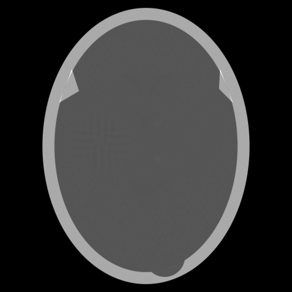
(a)

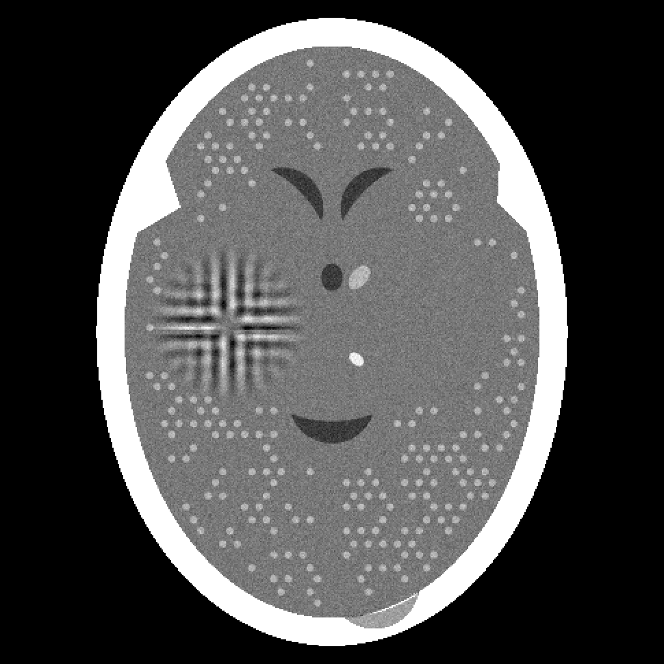
(b)

Figure 1: A $485\times 485$ digitization of a phantom based on the distribution of x-ray attenuation in units of cm^-1 within a transaxial slice of the human head. We display in (a) 0.000 as black and any value that is 0.6241749 or greater as white, in (b) 0.20400 as black and any value that is 0.21675 or greater as white. The latter mapping of values into displayed intensities is used for all the images shown below.

4 Experiments and Analysis

In this section we report on experiments with phantoms based on a transaxial slice of the human head. The phantoms mimic an actual medical image; for details, see Sections 4.3 and 4.4 of [1]. The various phantoms differ from each other by the random assignment of local inhomogeneities and, more importantly, by a random introduction of small “tumors”; see Section 5.2 of [1]. A $485\times 485$ digitization of one such phantom (produced by the software SNARK14 [26] in the manner specified in [1]) is shown in Fig. 1. In this, and in all of the other digitized images shown in this paper, the length of a side of a pixel is 0.0376 cm.

4.1 Comparison Using Single Data Sets

We first describe an anecdotal experiment that compares outputs of the classical methods of filtered back-projection (FBP) [1, Chapter 10] and the algorithm ART with the reconstruction algorithms that are discussed in the previous section; namely, the TV-Based Superiorized Version of ART and the Shearlet-Based Superiorized Version of ART. To make these comparisons, we applied the algorithms to CT problems using the phantom of Fig. 1. In the simulated CT scanner, the acquisition process generated divergent projection data, with source-to-detector distance 110.735 cm and source-to-center-of-rotation distance 78 cm, over view angles with 693 rays per view, with a detector spacing of 0.0533 cm. The projection data were simulated using integrals over the original structures rather than over digitized versions of them. The stochastic nature of the data collection is simulated by using 1,000,000 photons for estimating each line integral. The phantom and data acquisition were generated using the software SNARK14 [26]. The SNARK14 software allows the modeling of beam hardening that would be experienced in a real CT scanner (for exact details, see the description of the standard projection data in Section 5.8 of [1]), but here we did not make use of this feature. The SNARK14 software was also used for implementing the various reconstruction algorithms in the experiments.

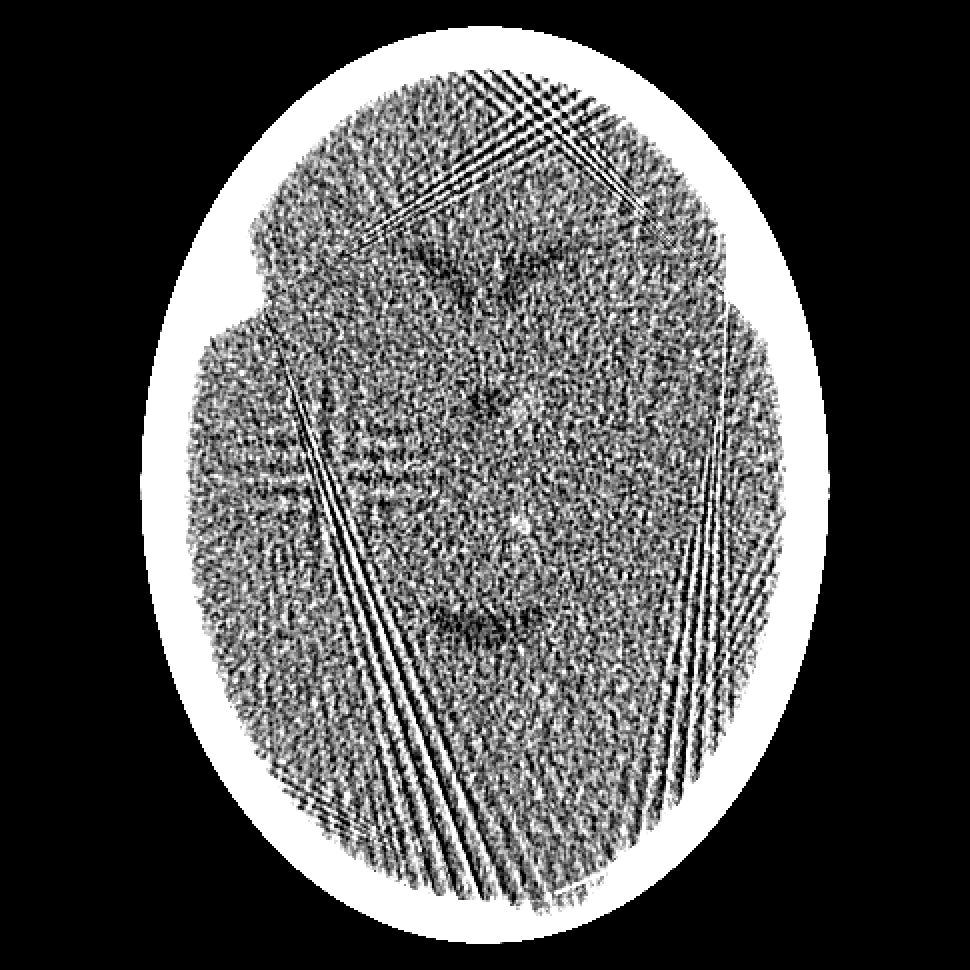
(a)

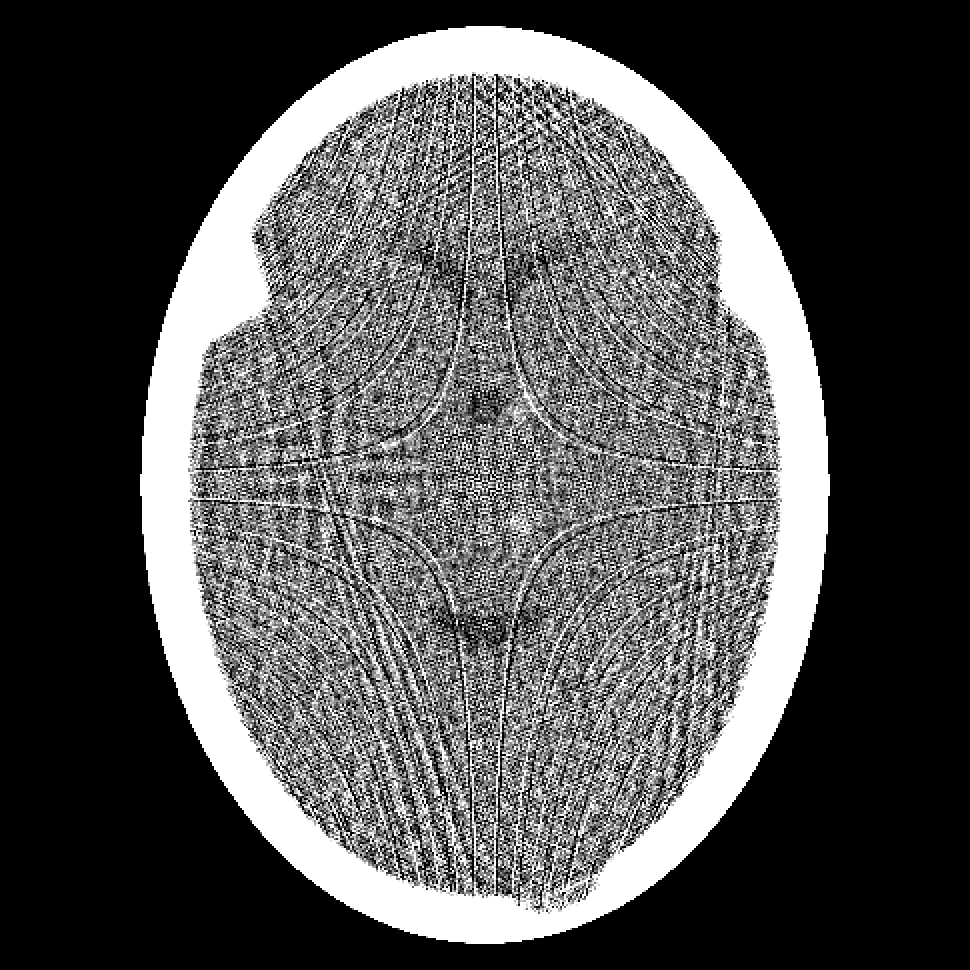
(b)

(c)

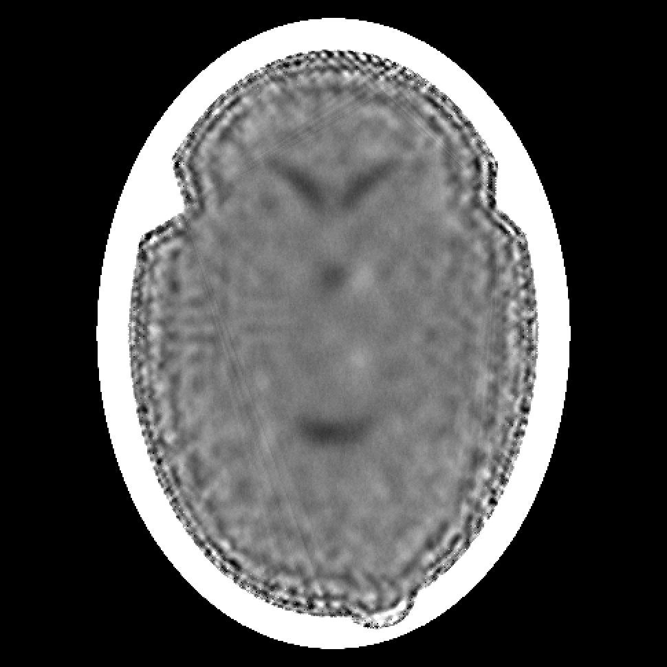
(d)

Figure 2: Reconstructions from 180 projections by (a) filtered back-projection, (b) the algorithm ART, (c) TV-Based Superiorized Version of ART, and (d) Shearlet-Based Superiorized Version of ART.

(a)

(b)

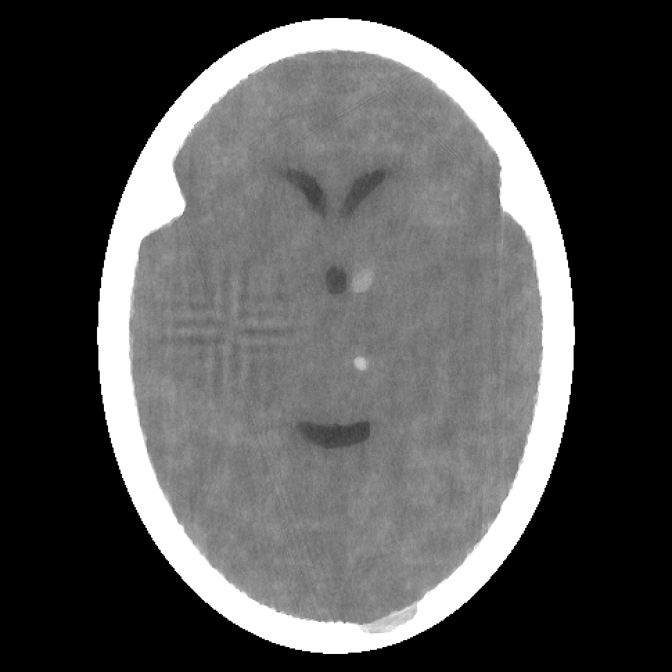
(c)

(d)

Figure 3: Reconstructions from 360 projections by (a) filtered back-projection, (b) the algorithm ART, (c) TV-Based Superiorized Version of ART, and (d) Shearlet-Based Superiorized Version of ART.

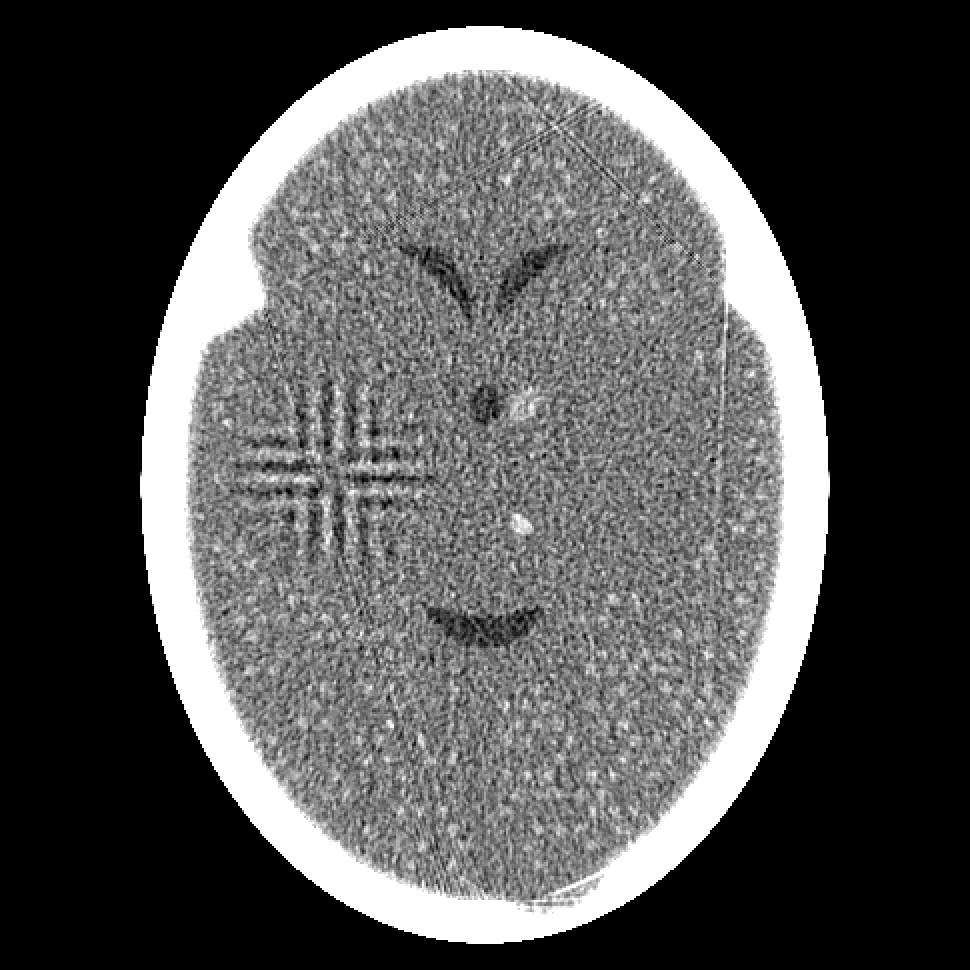
(a)

(b)

(c)

(d)

Figure 4: Reconstructions from 720 projections by (a) filtered back-projection, (b) the algorithm ART, (c) TV-Based Superiorized Version of ART, and (d) Shearlet-Based Superiorized Version of ART.

For this anecdotal experiment we use three different numbers of views (i.e., projections): 180, 360, and 720. We emphasize that, in the currently-described anecdotal experiment, there is only one phantom (which provides the ground truth); random generation of local inhomogeneities and of tumor locations is done only once and the same arrangement of local inhomogeneities and of tumor locations is used when generating the projection data for the three different numbers of views.

The details of the reconstruction algorithms that we compare are as follows. The specific choices are based on published results and some preliminary experiments.

• For the filtered back-projection (FBP) method [1, Chapter 10], we used the sinc window with linear interpolation (also called the Shepp-Logan window).

• Each of the three iterative algorithms returns as its output the vector $\boldsymbol{x}^{(k)}$ for the smallest value of $k$ such that $\left\|\boldsymbol{y}-\mathbf{R}\boldsymbol{x}^{(k)}\right\|_{2}\leq\left\|\boldsymbol{y}-\mathbf{R}\boldsymbol{x}\right\|_{2}$, where $\boldsymbol{x}$ is the output returned by FBP for the same projection data $\boldsymbol{y}$.

• For the two superiorized versions of ART, we used the values of 0.03 for $\beta_{0}$, 0.9999 for $\alpha$, 0.05 for $\rho$, 40 for $N$, and $10^{-20}$ for $\zeta$.

We present the visual results of the reconstructions produced by these algorithms when using 180, 360, and 720 projections in Figures 2, 3, and 4, respectively. We now give our impressions based on these visual results.

From the results for the single data set with 180 projections (Figure 2), we see that none of the four reconstruction algorithms produces an image in which the small tumors are easily locatable. Furthermore, the Shearlet-Based Superiorized Version of ART introduces high frequency artifacts in the brain near the skull and blurs the features inside the brain. In comparison, both filtered back-projection and ART (to a lesser extent) introduce artifacts in the form of streaks originating from interior bone edges. The image produced by TV-superiorized ART does not show significant high-frequency artifacts, the only one of the four, but the image is blurred.

In the case of 360 projections, the resulting images still show that none of the algorithms provides clear visualization of the small tumors; although they are somewhat visible in the images produced by filtered back-projection and by ART. The Shearlet-Based Superiorized Version of ART still shows high-frequency artifacts, albeit less pronounced than in the case of 180 projections. TV-superiorized ART produces an image in which the features, especially the small tumors, are smoothed out, but the larger features within the brain are clearly identifiable.

As expected, the greater are the number of projections, the better are the reconstructions produced by any of the four algorithms. However, even with 720 projections, the reconstruction produced by the Shearlet-Based Superiorized Version of ART still shows some high-frequency artifacts and the small tumors are less visible than in the images produced by the other three algorithms.

To supplement the just-listed visual impressions with numerical results, we computed the residual (i.e., $\left\|\boldsymbol{y}-\mathbf{R}\boldsymbol{x}\right\|_{2}$), the total variation (i.e., $\Upsilon\left(\boldsymbol{x}\right)$), and the $\ell_{1}$-norm of the shearlet transform (i.e., $\left\|\mathbf{S}\boldsymbol{x}\right\|_{1}$) for all the reconstructions produced by the algorithms when using 180, 360, and 720 projections; we present these values in Table 1. The entries in the table indicate that the presented superiorized versions manifest what is expected from them: For all three data sets, the value of $\Upsilon\left(\boldsymbol{x}\right)$ for the $\boldsymbol{x}$ produced by the TV-Based Superiorized Version of ART is smaller than the value of $\Upsilon\left(\boldsymbol{x}\right)$ for the $\boldsymbol{x}$ produced by any of the other three algorithms and the value of $\left\|\mathbf{S}\boldsymbol{x}\right\|_{1}$ for the $\boldsymbol{x}$ produced by the Shearlet-Based Superiorized Version of ART is smaller than the value of $\left\|\mathbf{S}\boldsymbol{x}\right\|_{1}$ for the $\boldsymbol{x}$ produced by any of the other three algorithms.

# of	Measure	FBP	ART	Superiorized	Superiorized
Angles				ART $\Upsilon\left(\boldsymbol{x}\right)$	ART $\left\|\mathbf{S}\boldsymbol{x}^{\left(k\right)}\right\|_{1}$
180	$\left\|\boldsymbol{y}-\mathbf{R}\boldsymbol{x}\right\|_{2}$	3.6380	3.6088	3.5389	3.6235
	$\Upsilon\left(\boldsymbol{x}\right)$	3,007.6751	3,565.0785	926.5716	1,261.0999
	$\left\|\mathbf{S}\boldsymbol{x}\right\|_{1}$	7,289.0860	6,779.7905	4,935.8958	4,673.0563
360	$\left\|\boldsymbol{y}-\mathbf{R}\boldsymbol{x}\right\|_{2}$	4.0314	3.9267	3.9089	4.0075
	$\Upsilon\left(\boldsymbol{x}\right)$	1,797.8089	3,259.0070	955.4895	1,268.0752
	$\left\|\mathbf{S}\boldsymbol{x}\right\|_{1}$	5,840.9464	6,672.6732	5,278.3972	5,031.3871
720	$\left\|\boldsymbol{y}-\mathbf{R}\boldsymbol{x}\right\|_{2}$	5.9793	5.3769	5.7150	5.7747
	$\Upsilon\left(\boldsymbol{x}\right)$	1,331.3471	2,900.1962	1,016.4190	1,346.1710
	$\left\|\mathbf{S}\boldsymbol{x}\right\|_{1}$	5,389.4274	6,444.8295	5,227.6876	5,147.9080

Table 1: Computed values for the residual (i.e., $\left\|\boldsymbol{y}-\mathbf{R}\boldsymbol{x}\right\|_{2}$), the total variation (i.e., $\Upsilon\left(\boldsymbol{x}\right)$), and the $\ell_{1}$-norm of the shearlet transform (i.e., $\left\|\mathbf{S}\boldsymbol{x}\right\|_{1}$) for all the reconstructions produced by filtered back-projection (FBP), the algorithm ART, the TV-Based Superiorized Version of ART (using $\Upsilon\left(\boldsymbol{x}\right)$), and the Shearlet-Based Superiorized Version of ART (using $\left\|\mathbf{S}\boldsymbol{x}\right\|_{1})$, for 180, 360, and 720 projection angles.

That the mathematical behavior of the algorithms is as expected indicates the correctness of the theory and the programming, but says nothing about the relative efficacy in practice of using TV or shearlets for the secondary criterion. We now turn to discussing this topic.

First we analyze the anecdotal experiment from this point of view. One figure of merit for the efficacy of a reconstruction algorithm is the relative error, which is a normalized mean absolute distance measure [1, equation (5.2)]. In our current notation it is defined as

$$r=\left\|\mathbf{p}-\boldsymbol{x}\right\|_{1}/\left\|\mathbf{p}\right\|_{1},$$ (9)

where $\boldsymbol{p}$ is the phantom and $\boldsymbol{x}$ is the reconstruction.

In Fig. 5 we report on the relative errors for the data sets of 180 and 720 views. In both cases the red dot (with the dashed line) indicates the value of the relative error obtained by FBP (a noniterative algorithm). For the iterative algorithms, we report on the relative error for $\boldsymbol{x}=\boldsymbol{x}^{(k)}$, where $k$ is the iteration number. We see that, for both data sets, the TV-Based Superiorized Version of ART outperforms the Shearlet-Based Superiorized Version of ART, at least when performance is measured by the relative error $r$. Both superiorized versions outperform the unsuperiorized algorithm ART. The same is true for the data set for 360 views; we are not illustrating that in this paper.

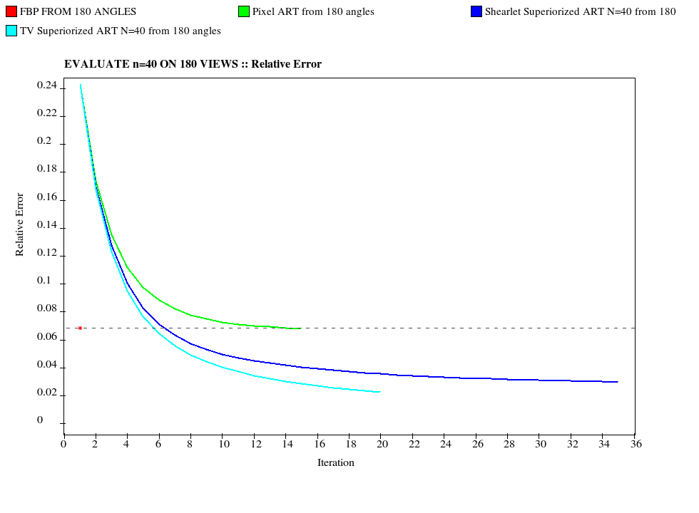
(a)

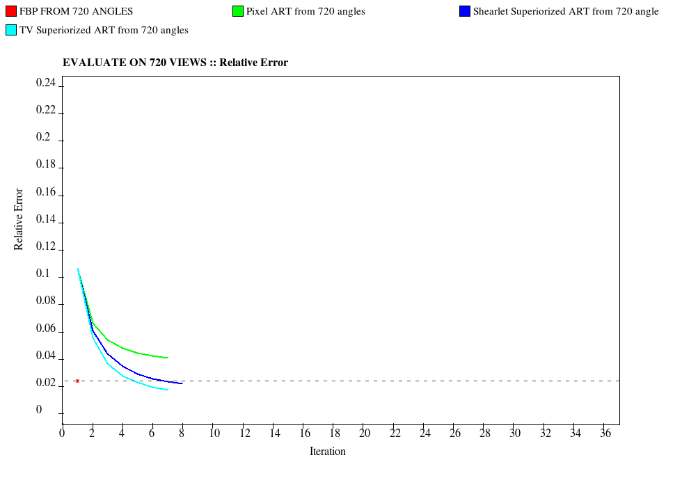
(b)

Figure 5: The relative errors (9) of the reconstructions produced by the four algorithms for two data sets: (a) 180 projections and (b) 720 projections.

4.2 Statistical Comparison

In order to draw firm conclusions about the relative efficacy of the four reconstruction algorithms, we complement our report based on single data sets with other experiments that use statistical hypothesis testing (SHT) for task-oriented comparisons [1, Section 5.2] of them. Similarly to the experiments for the single data sets, we used three different number of projections (180, 360, 720) for the SHT experiments. The reported results were obtained by SNARK14 using its “experimenter” feature [26, Chapter 8].

Our SHT experiments consist of the following four steps: (i) Generation of samples from an ensemble of phantoms of the kind described at the beginning of this Section 4. The ensemble is based on a transaxial slice of the human head with local inhomogeneities. Note that this by itself provides us a statistical ensemble because the local inhomogeneities are introduced using a Gaussian random variable. However there is an additional (for the task more relevant) variability within the ensemble that is achieved as follows. We specify a large number of pairs of potential tumor sites, the locations of the sites in a pair are symmetrically placed in the left and right halves of the brain. In any sample from the ensemble, exactly one of each pair of the sites will actually have a tumor placed there, with equal probability for either site. In Fig. 1(b) we illustrate one sample from this ensemble (i.e., one of the phantoms with random allocation of the tumors to the potential sites). (ii) Generation of realistic projection data sets, by using the parameters specified for the CT simulator (this introduces extra randomness due to the quantum noise in the data generation) for every randomly-generated phantom and using them to produce reconstructions with the reconstruction algorithms. (iii) Measuring the goodness of every reconstruction by using a medically-relevant figure of merit (FOM). (iv) Computation of the statistical significance (based on the FOMs of all the reconstructions for all the data sets) by which the null hypothesis that a pair of algorithms is equally good can be rejected in favor of the alternative hypothesis that the reconstruction algorithm with the higher average value of the FOM (call this Algorithm 1) is better than reconstruction algorithm with the lower average value of the FOM (call this Algorithm 2).

In order to obtain statistically significant results, we sampled the ensemble of phantoms and generated projection data 30 times. For each of the thirty projection data sets, we subtracted from the FOM of the reconstruction produced by Algorithm 1 the FOM of the reconstruction produced by Algorithm 2. (Note that the null hypothesis of equal efficacy of the two algorithms would imply that the expected value of this difference is zero.) We define $s$ as the average of these differences over the thirty data sets. There is a method (for details, see [1, Section 5.2)]) for estimating the so-called P-value, which is the probability under the null hypothesis of obtaining a value for $s$ that is as large or larger than what we actually obtained in the experiment. If the null hypothesis were correct, we would not expect to come across an $s$ for which the P-value is very small. Thus, the smallness of the P-value is a measure of significance for rejecting the null hypothesis that the two reconstruction algorithms are equally good according to our selected FOM in favor of the alternative hypothesis that Algorithm 1 is better than Algorithm 2.

For all our SHT experiments we used the FOM called imagewise-region-of-interest (IROI) [1, 26, 27] that, for our experiments, is defined as follows. In our phantoms there are pairs of potential tumor locations in the brain; we index these pairs with $b=1,\ldots,B$. For each pair, just one of the locations contains a tumor, that increases the value of $f$ at that location. We define

$${\small\begin{array}[]{ll}\textrm{IROI}=&\left(\frac{\sum_{b=1}^{B}\left(\upsilon_{t}^{p}\left(b\right)-\upsilon_{n}^{p}\left(b\right)\right)}{\sqrt{\sum_{b=1}^{B}\left(\upsilon_{n}^{p}\left(b\right)-\frac{1}{B}\sum_{b^{\prime}=1}^{B}\upsilon_{n}^{p}\left(b^{\prime}\right)\right)^{2}}}\right)^{-1}\times\\ &\left(\frac{\sum_{b=1}^{B}\left(\upsilon_{t}^{r}\left(b\right)-\upsilon_{n}^{r}\left(b\right)\right)}{\sqrt{\sum_{b=1}^{B}\left(\upsilon_{n}^{r}\left(b\right)-\frac{1}{B}\sum_{b^{\prime}=1}^{B}\upsilon_{n}^{r}\left(b^{\prime}\right)\right)^{2}}}\right),\end{array}}$$ (10)

where $\upsilon_{t}^{p}\left(p\right)$ (respectively, $\upsilon_{n}^{p}\left(p\right)$) denotes the average density in the phantom of the structure of the $b$th pair that is (respectively, is not) the tumor. Similarly, the $\upsilon_{t}^{r}\left(p\right)$ (respectively, $\upsilon_{n}^{r}\left(p\right)$) denotes the average density in the reconstruction of the structure of the $b$th pair that is (respectively, is not) the tumor. If the reconstruction is perfect, in the sense of being identical to the phantom, then IROI=1. All the parameters, including the stopping criteria (provided by the $\varepsilon$), for the reconstructions from each of the 30 random data sets were the ones specified previously for the experiment using a single data sets.

By using SHT for task-oriented comparisons of the four reconstruction algorithms, with IROI as the figure of merit, we found that TV-superiorized ART always outperformed ART and Shearlet-Based Superiorized Version of ART with strong statistical significance (i.e., very small P-values), see Table 2. However, TV-superiorized ART only outperformed filtered back-projection in the experiment with 180 projections; in fact, in the other two experiments (i.e., 360 and 720 projections) filtered back-projection outperforms the other three algorithms with strong statistical significance, see Table 2. The conclusion that we can draw from this is that if the number of projections is not very small (i.e., 360 or more) and the medical task is the localization of very small tumors in the brain, then the secondary criterion of having a small TV is not the appropriate one for turning the algorithm ART into a superiorized version that outperforms FBP. This is because the smoothing property of this secondary criterion results in the very small tumors being blurred out in the reconstruction, as is illustrated very clearly in Fig. 3c. (We note that having a small $\left\|\mathbf{S}\boldsymbol{x}\right\|_{1}$ has proven to be an even less appropriate secondary criterion for this medical task.) On the positive side for TV as a secondary criterion, we note that, with 180 projections, the TV-based superiorized ART significantly outperforms the other three reconstruction algorithms.

# of	FBP	ART	Superiorized	Superiorized ART	P-value
Angles			ART $\Upsilon\left(\boldsymbol{x}\right)$	ART $\left\|\mathbf{S}\boldsymbol{x}\right\|_{1}$
180	0.070656	0.064593			${\scriptstyle 1.686016\times 10^{-6}}$
	0.070656		0.088268		${\scriptstyle 2.418553\times 10^{-7}}$
	0.070656			0.057435	${\scriptstyle 3.450878\times 10^{-7}}$
		0.064593	0.088268		${\scriptstyle 5.374371\times 10^{-8}}$
		0.064593		0.057435	${\scriptstyle 1.844853\times 10^{-6}}$
			0.088268	0.057435	${\scriptstyle 3.812557\times 10^{-8}}$
360	0.163389	0.126363			${\scriptstyle 3.799954\times 10^{-8}}$
	0.163389		0.152645		${\scriptstyle 1.702295\times 10^{-5}}$
	0.163389			0.103251	${\scriptstyle 3.425471\times 10^{-8}}$
		0.126363	0.152645		${\scriptstyle 6.196416\times 10^{-8}}$
		0.126363		0.103251	${\scriptstyle 8.772077\times 10^{-8}}$
			0.152645	0.103251	${\scriptstyle 3.464983\times 10^{-8}}$
720	0.235774	0.167454			${\scriptstyle 2.967738\times 10^{-8}}$
	0.235774		0.215847		${\scriptstyle 4.350362\times 10^{-7}}$
	0.235774			0.180246	${\scriptstyle 4.141425\times 10^{-8}}$
		0.167454	0.215847		${\scriptstyle 2.983396\times 10^{-8}}$
		0.167454		0.180246	${\scriptstyle 8.518713\times 10^{-6}}$
			0.215847	0.180246	${\scriptstyle 8.105134\times 10^{-8}}$

Table 2: Results of the statistical hypothesis testing (SHT) experiments that compared reconstructions produced by filtered back-projection (FBP), the algorithm ART, the TV-Based Superiorized Version of ART (using $\Upsilon\left(\boldsymbol{x}\right)$), and the Shearlet-Based Superiorized Version of ART (using $\left\|\mathbf{S}\boldsymbol{x}\right\|_{1})$, with IROI (10) as the figure of merit. The entries in the body of this table are the average values of IROI over the 30 random data sets.

5 The Split Bregman Approach

The authors of [12] use a modified split Bregman method with both the shearlet transform and total variation as regularization terms. In this section we discuss such approaches and compare their outputs against the superiorization method.

The CT problem of (3) can be converted into the regularized global optimization problem

$$\mathbf{Find}\;\boldsymbol{x}^{*}=\arg\underset{\boldsymbol{x}}{\min}\left(\frac{\kappa}{2}\left\|\boldsymbol{y}-\mathbf{R}\boldsymbol{x}\right\|_{2}^{2}+\phi\left(\boldsymbol{x}\right)\right),$$ (11)

where $\kappa$ is a positive-real-number parameter that controls the relative importance between the constraints-compatibility and the prior desirability; this parameter replaces the $\varepsilon$ of (3). An alternative way of describing the role of $\kappa$ is that it determines the contribution of the regularization term to the total cost (lower value of $\kappa$ results in larger contribution of the regularization term $\phi\left(\boldsymbol{x}\right)$). Formulations of both kinds (i.e., the ones of equations (3) and (11)) are listed in the beginning parts of [28]; see also [29].

The split Bregman method is an iterative procedure that, in addition to producing a sequence $\boldsymbol{x}^{\left(k\right)}$ of $J$-dimensional vectors that are supposed to converge to $\boldsymbol{x}^{*}$ of (11), also produces two auxiliary sequences $\boldsymbol{q}^{\left(k\right)}$ and $\boldsymbol{b}^{\left(k\right)}$ of $I$-dimensional vectors according to the following recurrence rules. We set $\boldsymbol{x}^{\left(0\right)}$, $\boldsymbol{q}^{\left(0\right)}$ and $\boldsymbol{b}^{\left(0\right)}$ to be vectors (each of them denoted by $\mathbf{0})$ all of whose components are zero. For all nonnegative integers $k$, we define

$$\boldsymbol{x}^{\left(k+1\right)}=\arg\underset{\boldsymbol{x}}{\min}\left(\frac{\kappa}{2}\left\|\boldsymbol{y}-\mathbf{R}\boldsymbol{x}\right\|_{2}^{2}+\frac{\mu}{2}\left\|\boldsymbol{q}^{\left(k\right)}-\phi\left(\boldsymbol{x}^{(k)}\right)-\boldsymbol{b}^{\left(k\right)}\right\|_{2}^{2}\right),$$ (12)

where $\mu$ is a fixed positive-real-number relaxation parameter,

$$\boldsymbol{q}^{\left(k+1\right)}=\arg\underset{\boldsymbol{q}}{\min}\left(\left\|\boldsymbol{q}\right\|_{1}+\frac{\mu}{2}\left\|\boldsymbol{q}-\phi\left(\boldsymbol{x}^{(k+1)}\right)-\boldsymbol{b}^{\left(k\right)}\right\|_{2}^{2}\right),$$ (13)

$$\boldsymbol{b}^{\left(k+1\right)}=\boldsymbol{b}^{\left(k\right)}+\left(\phi\left(\boldsymbol{x}^{(k+1)}\right)-\boldsymbol{q}^{\left(k+1\right)}\right).$$ (14)

5.1 Using the $\ell_{1}$-Norm of the Shearlet Transform

The authors of [12] propose replacing $\phi\left(\boldsymbol{x}\right)$ by $\left\|\mathbf{S}\boldsymbol{x}\right\|_{1}$ in (11), resulting in equations (12), (13) and (14) becoming

$$\boldsymbol{x}^{\left(k+1\right)}=\arg\underset{\boldsymbol{x}}{\min}\left(\frac{\kappa}{2}\left\|\boldsymbol{y}-\mathbf{R}\boldsymbol{x}\right\|_{2}^{2}+\frac{\mu}{2}\left\|\boldsymbol{q}^{\left(k\right)}-\mathbf{S}\boldsymbol{x}^{(k)}-\boldsymbol{b}^{\left(k\right)}\right\|_{2}^{2}\right),$$ (15)

$$\boldsymbol{q}^{\left(k+1\right)}=\arg\underset{\boldsymbol{q}}{\min}\left(\left\|\boldsymbol{q}\right\|_{1}+\frac{\mu}{2}\left\|\boldsymbol{q}-\mathbf{S}\boldsymbol{x}^{(k+1)}-\boldsymbol{b}^{\left(k\right)}\right\|_{2}^{2}\right),$$ (16)

$$\boldsymbol{b}^{\left(k+1\right)}=\boldsymbol{b}^{\left(k\right)}+\left(\mathbf{S}\boldsymbol{x}^{(k+1)}-\boldsymbol{q}^{\left(k+1\right)}\right),$$ (17)

respectively.

By taking the derivatives of the right hand side of (15), we see that the $\boldsymbol{x}^{\left(k+1\right)}$ of (15) satisfies

$$\mathbf{R}^{\dagger}\left(\boldsymbol{y}-\mathbf{R}\boldsymbol{x}\right)+\frac{\mu}{\kappa}\left[\mathbf{S}^{\dagger}\left(\boldsymbol{q}^{\left(k\right)}-\mathbf{S}\boldsymbol{x}^{(k+1)}-\boldsymbol{b}^{\left(k\right)}\right)\right]=0,$$ (18)

where $\mathbf{R}^{\dagger}$ and $\mathbf{S}^{\dagger}$ are the transposes of the matrices $\mathbf{R}$ and $\mathbf{S}$, respectively. After regrouping we get ($\mathbf{I}$ is the $J\times J$ identity matrix):

$$\left(\mathbf{R}^{\dagger}\mathbf{R}+\frac{\mu}{\kappa}\mathbf{I}\right)\boldsymbol{x}^{(k+1)}=\mathbf{R}^{\dagger}\boldsymbol{y}+\frac{\mu}{\kappa}\mathbf{S}^{\dagger}\left(\boldsymbol{q}^{\left(k\right)}-\boldsymbol{b}^{\left(k\right)}\right).$$ (19)

The matrix $\left(\mathbf{R}^{\dagger}\mathbf{R}+\frac{\mu}{\kappa}\mathbf{I}\right)$ is positive definite (and, hence, invertible), but it is very large. For reasons of computational cost, it makes sense in practice to approximate $\boldsymbol{x}^{\left(k+1\right)}$ by applying a fixed limited number $M$ of iterations of the method of conjugate gradients [30] to solve (19) for $\boldsymbol{x}^{(k+1)}$. A single iterative step of the method is provided by the procedure Conjugate_Gradients$\left(\mathbf{P},\boldsymbol{u},\boldsymbol{v},\boldsymbol{w},\boldsymbol{u^{\prime}},\boldsymbol{v^{\prime}},\boldsymbol{w^{\prime}}\right)$, where $\mathbf{P}$ is a $J\times J$ matrix, $\boldsymbol{u},\boldsymbol{v},\boldsymbol{w}$ are $J$-dimensional input vectors and $\boldsymbol{u^{\prime}},\boldsymbol{v^{\prime}},\boldsymbol{w^{\prime}}$ are $J$-dimensional output vectors. Following [1, p. 231], the details of this procedure are:

1:  procedure Conjugate_Gradients$\left(\mathbf{P},\right.$$\boldsymbol{u},$$\boldsymbol{v},$$\boldsymbol{w},$$\boldsymbol{u^{\prime}},$ $\boldsymbol{v^{\prime}},$ $\left.\boldsymbol{w^{\prime}}\right)$

2:      set $\gamma\leftarrow\frac{\left\langle\boldsymbol{v},\boldsymbol{v}\right\rangle}{\left\langle\boldsymbol{w},\mathbf{P}\boldsymbol{w}\right\rangle}$

3:      set $\boldsymbol{u^{\prime}}\leftarrow\boldsymbol{u}+\gamma\boldsymbol{w}$

4:      set $\boldsymbol{v^{\prime}}\leftarrow\boldsymbol{v}-\gamma\mathbf{P}\boldsymbol{w}$

5:      set $\delta\leftarrow\frac{\left\langle\boldsymbol{v^{\prime}},\boldsymbol{v^{\prime}}\right\rangle}{\left\langle\boldsymbol{v},\boldsymbol{v}\right\rangle}$

6:      set $\boldsymbol{w^{\prime}}\leftarrow\boldsymbol{v^{\prime}}+\delta\boldsymbol{w}$

7:  end procedure

If we wish to approximate a solution of the system of equations $\mathbf{P}\boldsymbol{u=z}$, then this can be achieved by first setting $\boldsymbol{u}^{(0)}$ to an arbitrary $J$-dimensional vector, $\boldsymbol{v}^{(0)}$ and $\boldsymbol{w}^{(0)}$ to $\boldsymbol{z}-\mathbf{P}\boldsymbol{u}^{(0)}$ and then repeatedly iterating using Conjugate_Gradients$\left(\mathbf{P},\boldsymbol{u}^{(k)},\boldsymbol{v}^{(k)},\boldsymbol{w}^{(k)},\boldsymbol{u}^{(k+1)},\boldsymbol{v}^{(k+1)},\boldsymbol{w}^{(k+1)}\right)$. For a sufficiently large $K$, $\boldsymbol{u}^{(K)}$ will be a good approximation to the desired solution.

In [28] the solution to (16) makes use of a procedure that implements the so-called soft shrinkage operation that, when applied to an $I$-dimensional vector, produces an $I$-dimensional vector with a smaller $\ell_{1}$-norm. This procedure is Soft_Shrink$\left(\tau,\boldsymbol{a},\boldsymbol{c}\right)$, where $\tau$ is a nonnegative real-valued input parameter; $\boldsymbol{a}=\left(a_{0},a_{1},\cdots,a_{I-1}\right)^{T}$ is an $I$-dimensional input vector and $\boldsymbol{c}$ is an $I$-dimensional output vector. We use $\left|a\right|$ to denote the magnitude of the number $a$. The details of this procedure are:

1:  procedure Soft_Shrink$\left(\tau,\boldsymbol{a},\boldsymbol{c}\right)$

2:      for $i\leftarrow 0$ to $I-1$ do

3:           if $\left|a_{i}\right|>\tau$ then

4:              set $c_{i}\leftarrow\left(1-\frac{\tau}{\left|a_{i}\right|}\right)a_{i}$

5:           else

6:              set $c_{i}\leftarrow 0$

7:  end procedure

Under the conditions stated for the parameters of Soft_Shrink$\left(\tau,\boldsymbol{a},\boldsymbol{c}\right)$, it will always be the case that $\left\|\boldsymbol{c}\right\|_{1}\leq\left\|\boldsymbol{a}\right\|_{1}$, with the inequality strict unless all components of $\boldsymbol{a}$ are zero or $\tau$ is zero. The use of the softshrink operator is feasible because there is no coupling between the elements of $\boldsymbol{c}$.

Based on this we can now state the algorithm proposed in [12]. The user-specified input parameters to this algorithm are the $\kappa$, $\mu$, $M$ and $K$ (the number of iterations).

Algorithm 2 Modified Split Bregman Algorithm

1:  set $k\leftarrow 0$

2:  set $\boldsymbol{x}^{\left(0\right)}\leftarrow\mathbf{0}$

3:  set $\boldsymbol{q}^{\left(0\right)}\leftarrow\mathbf{0}$

4:  set $\boldsymbol{b}^{\left(0\right)}\leftarrow\mathbf{0}$

5:  while $k<K$

6:       set $m\leftarrow 0$

7:       set $\boldsymbol{u}^{\left(0\right)}\leftarrow\boldsymbol{x}^{\left(k\right)}$

8:       set $\boldsymbol{v}^{\left(0\right)}$$\leftarrow$$\mathbf{R}^{\dagger}\boldsymbol{y}$$+$$\frac{\mu}{\kappa}\mathbf{S^{\dagger}}\left(\boldsymbol{q}^{\left(k\right)}-\boldsymbol{b}^{\left(k\right)}\right)$$-$$\left(\mathbf{R}^{\dagger}\mathbf{R}+\frac{\mu}{\kappa}\mathbf{I}\right)\boldsymbol{u}^{\left(0\right)}$

9:       set $\boldsymbol{w}^{\left(0\right)}\leftarrow\boldsymbol{v}^{\left(0\right)}$

10:       while $m<M$

11:            call Conjugate_Gradients$\left(\mathbf{R}^{\dagger}\mathbf{R}+\frac{\mu}{\kappa}\mathbf{I},\right.$$\boldsymbol{u}^{(m)},$$\boldsymbol{v}^{(m)},$$\boldsymbol{w}^{(m)},$                                                       $\boldsymbol{u}^{(m+1)},$$\boldsymbol{v}^{(m+1)},$$\left.\boldsymbol{w}^{(m+1)}\right)$

12:            set $m\leftarrow m+1$

13:       set $\boldsymbol{x}^{\left(k+1\right)}\leftarrow\boldsymbol{u}^{\left(M\right)}$

14:       set $\boldsymbol{a}\leftarrow\mathbf{S}\boldsymbol{x}^{(k+1)}+\boldsymbol{b}^{\left(k\right)}$

15:       call Soft_Shrink$\left(\frac{1}{\mu},\boldsymbol{a},\boldsymbol{q}^{(k+1)}\right)$

16:       set $\boldsymbol{b}^{(k+1)}\leftarrow\boldsymbol{b}^{\left(k\right)}+\left(\mathbf{S}\boldsymbol{x}^{(k+1)}-\boldsymbol{q}^{\left(k+1\right)}\right)$

17:       set $k\leftarrow k+1$

18:  return $\boldsymbol{x}^{\left(K\right)}$

We compared the performance of the Shearlet-Based Superiorized Version of ART with that of the Modified Split Bregman Algorithm on the projection data used in Subsection 4.1; the relative errors are reported in Fig. 6. In Fig. 7 we show the results of the two approaches after the third and the tenth iteration.

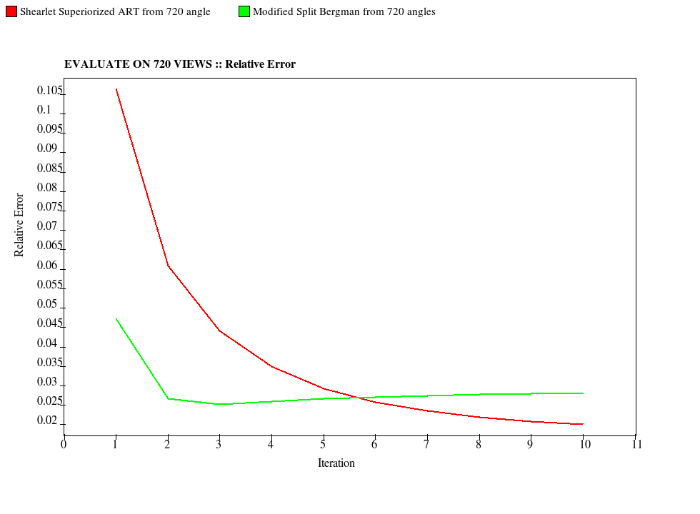
Figure 6: The relative errors (9) of the reconstructions produced by the Shearlet-Based Superiorized Version of ART and the Modified Split Bregman algorithms for the data set with 720 projections.

(a)

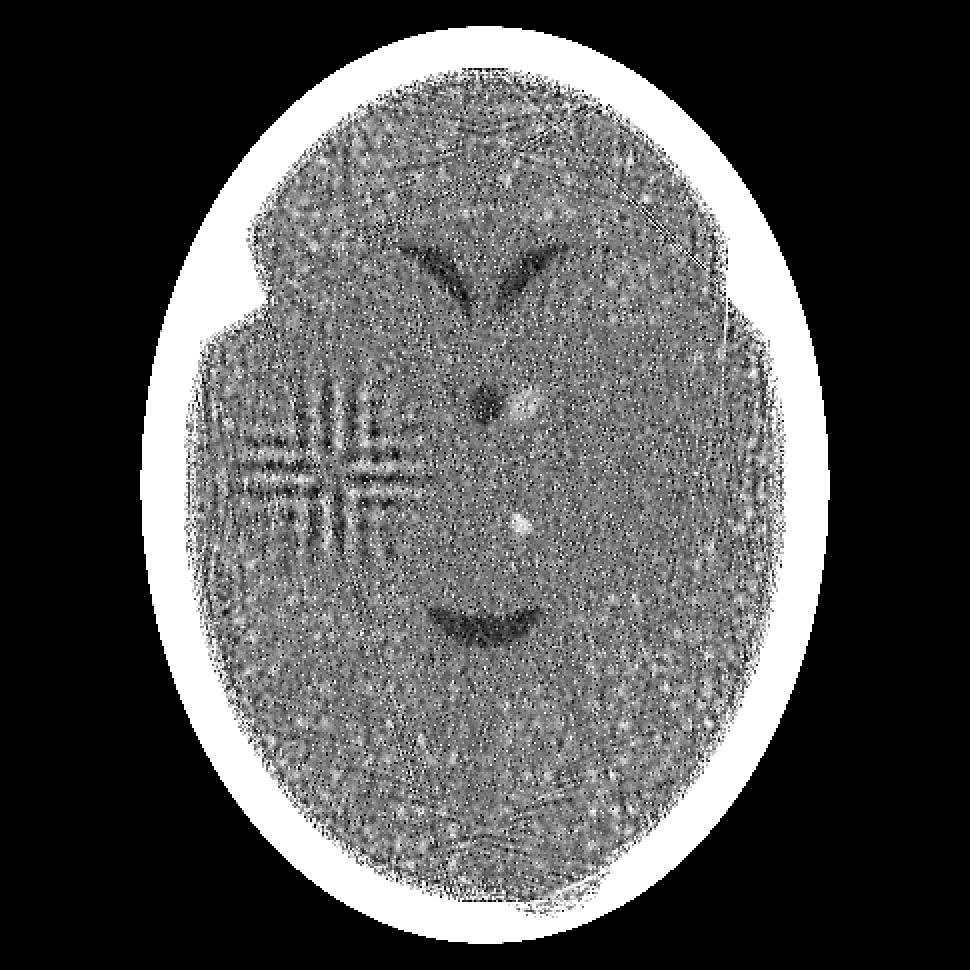
(b)

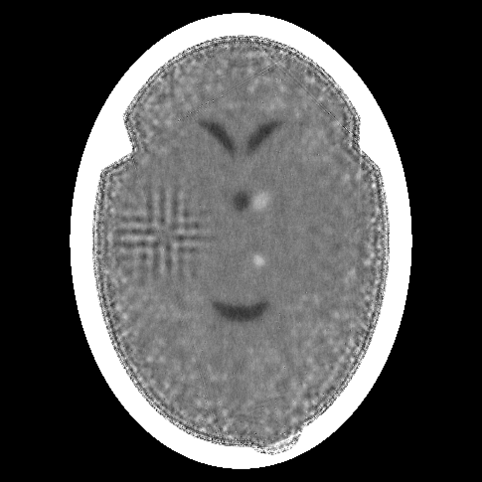
(c)

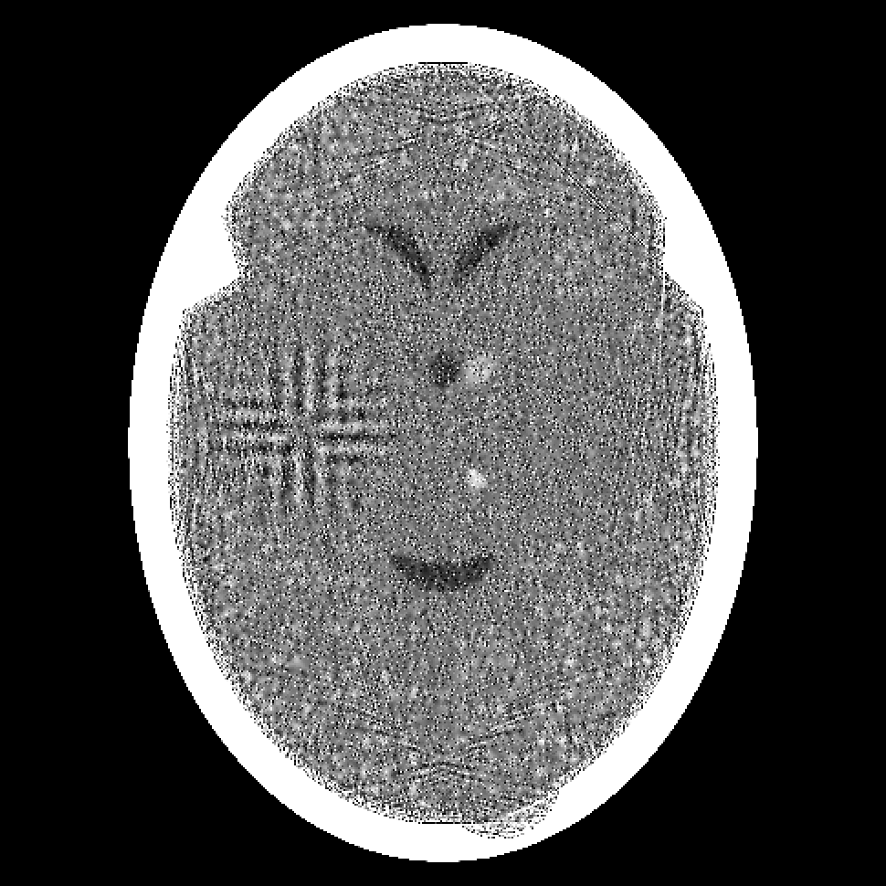
(d)

Figure 7: Results of the Shearlet-Based Superiorized Version of ART (left column) and the Modified Split Bregman Algorithm (right column) after the third (top row) and the tenth (bottom row) iteration from 720 projections.

5.2 Using Total Variation

We do not discuss the use of the split Bregman algorithm for TV in the same detail as we have done for $\ell_{1}$-norm of the shearlet transform, instead we just refer to an earlier work in which the topic is discussed. In [31] there is a comparison (see pp. 1082-3) of the performance of superiorization with that of a version of the split Bregman algorithm (suggested by T. Goldstein and S. Osher). In the reported experiment the performances of the two approaches are very similar according to both the primary and the secondary criterion, but superiorization reached its output four times faster than the split Bregman algorithm.

6 Discussion and Conclusions

The work on which we report above was originally motivated by the positive results in [12] on iterative CT reconstruction using shearlet-based regularization. We were particularly interested whether or not shearlet-based regularization is more efficacious than TV-based regularization (with which we had earlier positive experience) on the kind CT reconstructions problems the we have been using for the testing of reconstruction algorithms. For the purpose of this investigation we brought the two regularization approaches within a single framework using the methodology of superiorization. Making use of the general concept of the superiorization of an iterative algorithm, we have obtained Algorithm 1 that can be used for both TV-based and shearlet-based regularization. In that algorithm there is a need in Step 8 for obtaining a nonascending vector for the regularizing function (be that based on TV or shearlets, or whatever). Our actually implemented algorithms for TV-based and for shearlet-based regularization differ only in the procedures NonascendingTV and NonascendingShearlet that return a nonascending vector for TV and for shearlets, respectively. (The design of the second of these procedures is an original contribution of this paper, which is immediately applicable to finding nonascending vectors for any regularization criterion that is expressed as the $\ell_{1}$-norm of a transform specified by the application of a matrix.) Having developed this common framework, we could perform experiments comparing outcomes that depend only on the choice of the regularization, without any other differences in implementation and experimental design. In experiments reported above, TV-based superiorization turned out to be more efficacious than shearlet-based superiorization.

While this observation is quite firm based on the reported experiments, it is only fair to point out that it may be the case that, in spite of our best efforts, we have not succeeded to select the parameters of the Shearlet-Based Superiorized Version in an optimal manner. (An example of a possible improvement is to change the number scales in the fast Non-Iterative Shearlet Transform from the four, as specified near the end of Section 2, to five; we have not carried out a thorough investigation of the consequences of all such possible changes.) An extension of the Shearlet-Based Superiorized Version of ART, which includes both a TV term and a shearlet term (claimed to be beneficial as compared to using only either one of the two terms) was investigated in [32]. In our paper we compared the performance of algorithms in which just one of the terms is used.

We also reported comparisons of our superiorization approaches with two commonly-used CT reconstruction methods: FBP and (unsuperiorized) ART, as well as with the use of the split Bregman approach. The outcome of these comparisons is somewhat ambiguous. For example, TV-Based Superiorized ART was found better than FBP by all reported measures, except in the case when the number of projections is not very small (i.e., 360 or more) and the medical task that provides the figure of merit is the localization of very small tumors in the brain. On the other hand, TV-Based Superiorized ART was found better than unsuperiorized ART by all reported measures.

References

References

- [1] G. T. Herman, Fundamentals of Computerized Tomography: Image Reconstruction from Projections, 2nd ed. London, UK: Springer, 2009.
- [2] X. Pan, E. Y. Sidky, and M. Vannier, “Why do commercial CT scanners still employ traditional, filtered back-projection for image reconstruction?” Inverse Problems, vol. 25, p. 123009, 2009.
- [3] G. T. Herman and R. Davidi, “Image reconstruction from a small number of projections,” Inverse Problems, vol. 24, p. 045011, 2008.
- [4] G.-H. Chen, J. Tang, B. Nett, Z. Qi, S. Leng, and T. Szczykutowicz, “Prior image constrained compressed sensing (PICCS) and applications in X-ray computed tomography,” Current Medical Imaging Reviews, vol. 6, pp. 119 – 134, 2010.
- [5] H. Yu and G. Wang, “SART-type image reconstruction from a limited number of projections with the sparsity constraint,” International Journal of Biomedical Imaging, vol. 934847, p. 9, 2010.
- [6] J. Abascal, A. Sisniega, C. Chavarrías, J. J. Vaquero, M. Desco, and M. Abella, “Investigation of different Compressed Sensing approaches for respiratory gating in small animal CT,” in IEEE Nuclear Science Symposium and Medical Imaging Conference (NSS/MIC), Oct 2012, pp. 3344–3346.
- [7] E. J. Candès and D. L. Donoho, “Curvelets - A surprisingly effective nonadaptive representation for objects with edges,” in Curve and Surface Fitting, A. Cohen, C. Rabut, and L. Schumaker, Eds. Nashville, Tennessee, USA: Vanderbilt University Press, 1999, pp. 105 – 120.
- [8] P. Feng, B. Wei, Y. J. Pan, and D. L. Mi, “Construction of nonaliasing pyramidal transform,” Acta Electronica Sinica, vol. 37, pp. 2510 – 2514, 2009.
- [9] R. X. Gao and R. Yan, Wavelets: Theory and Applications for Manufacturing. New York: Springer, 2011.
- [10] G. Kutyniok, W.-Q. Lim, and X. Zhuang, “Digital shearlet transforms,” in Shearlets, G. Kutyniok and D. Labate, Eds. Boston, MA, USA: Birkhäuser, 2012, pp. 239 – 282.
- [11] S. Yi, D. Labate, G. R. Easley, and H. Krim, “A shearlet approach to edge analysis and detection,” IEEE Transactions on Image Processing, vol. 18, pp. 929 – 941, 2009.
- [12] B. Vandeghinste, B. Goossens, R. V. Holen, C. Vanhove, A. Pižurica, S. Vandenberghe, and S. Staelens, “Iterative CT reconstruction using shearlet-based regularization,” IEEE Transactions on Nuclear Science, vol. 60, pp. 3305 – 3317, 2013.
- [13] G. T. Herman, E. Garduño, R. Davidi, and Y. Censor, “Superiorization: An optimization heuristic for medical physics,” Medical Physics, vol. 39, pp. 5532 – 5546, 2012.
- [14] E. Garduño, G. T. Herman, and R. Davidi, “Reconstruction from a few projections by -minimization of the Haar transform,” Inverse Problems, vol. 27, no. 055006, 2011.
- [15] F. Natterer and F. Wübbeling, Mathematical Methods in Image Reconstruction. Philadelphia, PA, USA: Society for Industrial and Applied Mathematics (SIAM), 2001.
- [16] M. Beister, D. Kolditz, and W. A. Kalender, “Iterative reconstruction methods in X-ray CT,” Physica Medica, vol. 28, pp. 94 – 108, 2012.
- [17] E. J. Candès, J. Romberg, and T. Tao, “Robust uncertainty principles: exact signal reconstruction from highly incomplete frequency information,” IEEE Transactions on Information Theory, vol. 52, no. 2, pp. 489–509, Feb 2006.
- [18] Y. Censor, R. Davidi, and G. T. Herman, “Perturbation resilience and superiorization of iterative algorithms,” Inverse Problems, vol. 26, p. 065008, 2010.
- [19] D. Labate, W.-Q. Lim, G. Kutyniok, and G. Weiss, “Sparse multidimensional representation using shearlets,” Proceedings of the SPIE, vol. 5914, pp. 254 – 262, 2005.
- [20] G. R. Easley, D. Labate, and W.-Q. Lim, “Optimally sparse image representations using shearlets,” in Fortieth Asilomar Conference on Signals, Systems and Computers (ACSSC ’06), Pacific Grove, CA, 2006, pp. 974 – 978.
- [21] B. Goossens, J. Aelterman, H. Luong, A. Pižurica, and W. Philips, “Efficient design of a low redundant discrete shearlet transform,” in International Workshop on Local and Non-Local Approximation in Image Processing (LNLA 2009), Tuusula, Finland, 2009, pp. 112 – 124.
- [22] B. Goossens, J. Aelterman, Q. Luong, A. Pižurica, and W. Philips, “Design of a tight frame of 2D shearlets based on a fast non-iterative analysis and synthesis algorithm,” Proceedings of the SPIE, vol. 8138, pp. 1 – 13, 2011.
- [23] S. Häuser and G. Steidl, “Fast finite shearlet transform: A tutorial,” ArXiv, no. 1202.1773v2, 2014.
- [24] R. Gordon, R. Bender, and G. T. Herman, “Algebraic reconstruction techniques (ART) for three-dimensional electron microscopy and X-ray photography,” Journal of Theoretical Biology, vol. 29, pp. 471 – 481, 1970.
- [25] E. Garduño and G. T. Herman, “Superiorization of the ML-EM algorithm,” IEEE Transactions on Nuclear Science, vol. 61, pp. 162 – 172, 2014.
- [26] R. Davidi, G. T. Herman, O. Langthaler, S. Sardana, and Z. Ye, SNARK14: A Programming System for the Reconstruction of 2D Images from 1D Projections. [Online]. Available: http://www.dig.cs.gc.cuny.edu/software/snark14/SNARK14.pdf
- [27] T. K. Narayan and G. T. Herman, “Prediction of human observer performance by numerical observers: an experimental study,” Journal of the Optical Society of America A, vol. 16, pp. 679 – 693, 1999.
- [28] T. Goldstein and S. Osher, “The split Bregman method for L1-regularized problems,” SIAM Journal on Imaging Sciences, vol. 2, pp. 323 – 343, 2009.
- [29] M. Zibulevsky and M. Elad, “L1-L2 optimization in signal and image processing,” IEEE Signal Processing Magazine, vol. 27, no. 3, pp. 76 – 88, 2010.
- [30] M. R. Hestenes and E. Stiefel, “Methods of conjugate gradients for solving linear systems,” Journal of Research of the National Bureau of Standards, vol. 49, pp. 409 – 436, 1952.
- [31] Y. Censor, W. Chen, P. L. Combettes, R. Davidi, and G. T. Herman, “On the effectiveness of projection methods for convex feasibility problems with linear inequality constraints,” Computational Optimization and Applications, vol. 51, pp. 1065–1088, 2012.
- [32] B. Vandeghinste, B. Goossens, R. V. Holen, C. Vanhove, A. Pižurica, S. Vandenberghe, and S. Staelens, “Combined shearlet and TV regularization in sparse-view CT reconstruction,” in 2nd International Meeting on Image Formation in X-ray Computed Tomography, Utah, USA, 2012, pp. 24 – 27.