Abstract

We formalize a new statistical machine learning paradigm, called infinite-label learning, to annotate a data point with more than one relevant labels from a candidate set which pools both the finite labels observed at training and a potentially infinite number of previously unseen labels. The infinite-label learning fundamentally expands the scope of conventional multi-label learning and better meets the practical requirements in various real-world applications, such as image tagging, ads-query association, and article categorization. However, how can we learn a labeling function that is capable of assigning to a data point the labels omitted from the training set? To answer the question, we seek some clues from the recent works on zero-shot learning, where the key is to represent a class/label by a vector of semantic codes, as opposed to treating them as atomic labels. We validate the infinite-label learning by a PAC bound in theory and some empirical studies on both synthetic and real data.

1 Introduction

Recent years have witnessed a great surge of works on zero-shot learning [1, 2, 3, 4, 5, 6, 7, 8]. While conventional supervised learning methods (for classification problems) learn classifiers only for the classes that are supported by data examples in the training set, the zero-shot learning also strives to construct the classifiers of novel classes for which there is no training data at all. This is achieved by using class/label descriptors, often in the form of some vectors of numeric or symbolic values, in contrast to the atomic classes used in many other machine learning settings.

Zero-shot learning is appealing as it may bring machine learning closer to one of the remarkable human learning capabilities: generalizing learned concepts from old tasks to not only new data but also new (and yet similar) tasks [9, 10]. There are also many real-world applications for zero-shot learning. It facilitates cold-start [11] when the data of some classes are not available yet. In computer vision, the number of available images per object follows a long-tail distribution, and zero-shot learning becomes key to handling the rare classes. We note that the success of zero-shot learning largely depends on how much knowledge the label descriptors encode for relating the novel classes with the seen ones at training, as well as how the knowledge is involved in the decision making process, e.g., for classification.

Despite the extensive existing works on zero-shot learning for multi-class classifications, it is rarely studied for multi-label classification [12, 13, 14] except by [15, 16]. We contend that it is actually indispensable for multi-label learning algorithms to handle previously unseen labels. There are always new topics arising from the news (and research, education, etc.) articles over time. Creative hashtags could become popular on social networks over a night. There are about 53M tags on Flickr and many of them are associated with none or very few images. Furthermore, it is often laborious and costly to collect clean training data for the multi-label learning problems especially when there are many labels [17, 14]. To this end, we contend that zero-shot multi-label learning, which we call infinite-label learning to make it concise and interesting, is arguably a much more pressing need than the zero-shot multi-class classification.

To this end, we provide a formal treatment to the infinite-label learning problem in this paper. To the best of our knowledge, the two existing works [15, 16] on this problem only study specific application scenarios. Zhang et al. analyze the rankability of word embeddings [18, 19] and then use them to assign both seen and unseen tags to images [16]. Nam et al. propose a regularization technique for the WSABIE algorithm [20] to account for the label hierarchies [15]. In sharp contrast, we formalize the infinite-label learning as a general machine learning framework and show its feasibility both theoretically under some mild assumptions and empirically on synthetic and real data. Our results indicate that the infinite-label learning is hard and yet not impossible to solve, given appropriate semantic codes of the labels.

The semantic codes of the labels can be derived from a large knowledge base in addition to the training set. Thanks to the studies in linguistics, words in speech recognition are represented by combinations of phonemes [21]. In computer vision, an object class is defined by a set of visual attributes [5, 22]. More recently, the distributed representations of English words [18, 19] have found their applications in a variety of tasks. In biology, the labels are naturally represented by some structural or vectorial codes (e.g., protein structures [23]).

We organize the remaining of the paper as follows. We discuss some related work and machine learning settings next. After that, Section 3 formally states the problem of infinite-label learning, followed by some plausible modeling assumptions and algorithmic solutions. We then present a PAC-learning bound and some empirical results for this new machine learning framework in Sections 4 and 5, respectively. Section 6 concludes the paper.

2 Related work

We note that the semantic codes of labels have actually been used in various machine learning settings even before the zero-shot learning becomes popular [1, 2]. Bonilla et al.  use the vectorial representations of tasks to enrich the kernel function and parameterize a gating function [24]. Similarly, Bakker and Heskes input the task vectors to a neural network for task clustering and gating [25]. Wimalawarne et al. address multi-task learning when the tasks are each indexed by a pair of indices [26]. A large-margin algorithm is introduced in [27] to transform the classification problems to multivariate regression by considering the semantic codes of the classes as the target. It is worth pointing out that this line of works, unlike zero-shot learning or the infinite-label learning studied in this paper, lack the exploration of the learned models’ generalization capabilities to novel labels or tasks that are unseen in training.

Learning to rank [28, 29] and the cold-start problem in recommendation system [30, 31, 32] explicitly attempt to tackle unseen labels (e.g., queries and items, respectively) thanks to the label descriptions that are often vectorial. Zero-shot learning shares the same spirit [1, 2, 5, 3, 4, 7, 6, 8, 33, 34] and we particularly study the infinite-label learning in this paper.

Additionally, the semantic codes of labels or tasks also seamlessly unify a variety of machine learning settings  [35, 23]. The infinite-label learning studied in this paper can be regarded as a special case of the pairwise learning; in particular, a special case of the setting D in [23]. Nonetheless, we think the infinite-label learning is worth studying as a standalone machine learning framework given its huge application potentials. Besides, the PAC-learning analysis presented in this paper sheds light on the learnability of the pairwise learning [23].

The recent works of label embedding [36, 20, 37, 14] and landmark label sampling [38, 17] in multi-label learning are also related to our work. The main distinction is that their label representations are learned from the training set and are not applicable to unseen labels.

3 Infinite-label learning

The goal of infinite-label learning is to learn a decision function to annotate a data point with all relevant labels from a candidate set which pools both the finite labels observed at training and a potentially infinite number of previously unseen labels. In this section, we formally state the problem and then lay out a modeling assumption about the data generation process. We also provide some potential algorithmic solutions to the infinite-label learning.

Table 1: Multi-label learning vs. infinite-label learning.

	Multi-label learning	infinite-label learning (ZSML)
Data generation
Training data	$\mathcal{S}=\{(\bm{x}_{m},\bm{y}_{m})\}_{m=1}^{\mathsf{M}}$	$\mathcal{S},\;\mathcal{L}=\{\bm{\lambda}_{l}\}_{l=1}^{\mathsf{L}}$
Labeling function	$\bm{f}(\bm{x})\subseteq\mathcal{L}$	$\bm{f}(\bm{x})\subseteq\mathcal{L}\cup\mathcal{U}$, $\;\mathcal{U}=\{\bm{\lambda}_{l}\}_{l>\mathsf{L}}$
Example solution	$f_{l}(\bm{x})=\text{sgn}\left\langle\bm{w}_{l},\bm{x}\right\rangle,\;1\leq l\leq\mathsf{L}$	$f_{l}(\bm{x})=f({\bm{\lambda}}_{l};\bm{x})=\text{sgn}\left\langle V\bm{x},{\bm{\lambda}}_{l}\right\rangle,\;l\geq 1$

3.1 Problem statement

Suppose we have a set of vectorial labels $\mathcal{L}=\{\bm{\lambda}_{l}\in\mathbb{R}^{\mathsf{n}}\}_{l=1}^{\mathsf{L}}$ and a training sample $\mathcal{S}=\{(\bm{x}_{m},\bm{y}_{m})\in\mathbb{R}^{\mathsf{d}}\times\{-1,+1\}^{\mathsf{L}}\}_{m=1}^{\mathsf{M}}$, where the annotation $y_{ml}=+1$ indicates that the $l$-th label, which is described by $\bm{\lambda}_{l}$, is relevant to the $m$-th data point $\bm{x}_{m}$, and $y_{ml}=-1$ otherwise. For convenience, we refer to the label vectors $\mathcal{L}=\{\bm{\lambda}_{l}\}_{l=1}^{\mathsf{L}}$ as labels in the rest of the paper. Unlike conventional multi-label learning where one learns a decision function $\bm{f}({\bm{x}})\subseteq\mathcal{L}$ to assign the seen labels to an input data point, the infinite-label learning enables the decision function to additionally tag the data point with previously unseen labels $\mathcal{U}=\{\bm{\lambda}_{l}\}_{l>\mathsf{L}}$, where $\mathcal{L}\cap\mathcal{U}=\emptyset$.

Table 1 conceptually compares the infinite-label learning with multi-label learning. The rows of training data and labeling functions summarize the above discussions, and the other rows are elaborated in the next two subsections, respectively.

3.2 The non-i.i.d. training set

One of our objectives in this paper is to derive a PAC-learning bound for the infinite-label learning. To facilitate that, we carefully examine the data generation process in the infinite-label learning in this subsection.

At the first glance, one might impose a distribution $P_{X{\Lambda}Y}=P_{X{\Lambda}}P_{Y|X\Lambda}$ over the data $\bm{x}\sim X$, vectorial label $\bm{\lambda}\sim\Lambda$, and the indicator $y\sim Y|{\bm{x},\bm{\lambda}}$ about the relevance between the label and the data, and then assume the training sample ($\mathcal{S}$ and $\mathcal{L}$ jointly) is drawn i.i.d. from $P_{X{\Lambda}Y}$. Noting that $y$ implies nothing but a binary classification over the augmented data $(\bm{x},\bm{\lambda})$, the existing PAC-learning results could be used to bound the generalization error of the infinite-label learning.

The above reasoning is actually problematic because its corresponding generalization risk cannot be estimated empirically in real scenarios and applications. To see this point more clearly, we write out the generalization risk and its straightforward empirical estimate below,

$$R(h) =\mathbb{E}_{\bm{x},\bm{\lambda}\sim P_{X\Lambda}}\mathbb{E}_{y\sim P_{Y|\bm{x},\bm{\lambda}}}[h(\bm{x},\bm{\lambda})\neq y]$$ (1)

$$\widehat{R}_{\text{iid}}(h) =\frac{1}{\mathsf{M}}\sum_{m=1}^{\mathsf{M}}[h(\bm{x}_{m},\bm{\lambda}_{m})\neq y_{m}]$$ (2)

where $h\in\mathcal{H}$ is a hypothesis from a pre-fixed family $\mathcal{H}$ and $[\cdot]$ is the 0-1 loss. We can see that, under the i.i.d. assumption, the data and label $(\bm{x}_{m},\bm{\lambda}_{m})$ must be sampled simultaneously, i.e., they are exclusively coupled.

However, the seen labels and data in the training set are often pairwise examined and are not exclusively coupled. For example, to build the NUS-WIDE dataset [39], the annotators are asked to give the relevance between all the 81 tags and each image. Such practice instead suggests an alternative empirical risk,

$$\widehat{R}_{\text{non-iid}}(h)=\frac{1}{\mathsf{M}\mathsf{L}}\sum_{m=1}^{\mathsf{M}}\sum_{l=1}^{\mathsf{L}}[h(\bm{x}_{m},\bm{\lambda}_{l})\neq y_{ml}].$$

Moreover, the decoupling of data example $\bm{x}_{m}$ and label $\bm{\lambda}_{l}$ in $\widehat{R}_{\text{non-iid}}(h)$ also implies that the training set in infinite-label learning (and multi-label learning) is virtually generated from the joint distribution $P_{X{\Lambda}Y}$ in the following non-i.i.d. manner.

• Sample $\mathsf{M}$ times from $P_{X}$ and obtain $\{\bm{x}_{m}\}_{m=1}^{\mathsf{M}}$,

• Sample $\mathsf{L}$ times from $P_{\Lambda|\bm{x}_{1},\cdots,\bm{x}_{\mathsf{M}}}$ and obtain $\{\bm{\lambda}_{l}\}_{l=1}^{\mathsf{L}}$,

• Sample $y_{ml}$ from $P_{Y|\bm{x}_{m},\bm{\lambda}_{l}}$ for $m\in[\mathsf{M}],l\in[\mathsf{L}]$.

As a result, the training set is a non-i.i.d. sample drawn from $P_{X{\Lambda}Y}$. The existing PAC-learning bounds for binary classification cannot be directly applied here. Instead, we would like to bound the difference between the generalization risk $R(h)$ and the non-i.i.d. empirical risk $\widehat{R}_{\text{non-iid}}(h)$. To overcome this disparity is accordingly another contribution of this paper presented in Section 4.

Remarks.

We note that the joint distribution $P_{X\Lambda{Y}}$ is in general not sufficient to specify $P_{\Lambda|\bm{x}_{1},\cdots,\bm{x}_{\mathsf{M}}}$ appeared in the above sampling procedure. To rectify this, we make an independent assumption detailed in Section 4.

3.3 Views of the problem and algorithmic solutions

Given the sampling procedure described above, to solve infinite-label learning essentially is essentially to approximate the conditional distribution $P_{Y|X\Lambda}$. One potential hypothesis set for $P_{Y|X\Lambda}$ takes the simple bilinear form $f(\bm{x},\bm{\lambda})=\text{sgn}\left\langle V\bm{x},\bm{\lambda}\right\rangle$. Following the discussion about zero-data learning [1], we may understand this decision function from at least two views. From the data point of view, it is a decision function defined over the augmented input data, i.e., $(\bm{x},\bm{\lambda})$. From the model point of view, it defines a hyperplane $V\bm{x}$ that separates the labels $\bm{\lambda}\in\mathcal{L}\cup\mathcal{U}$ into two subsets no matter they are seen or unseen. One subset of the labels is relevant to the data instance $\bm{x}$ and the other is not, thanks to that the hyperplane is indexed by the input data. To learn the model parameters $V$, the maximum margin regression [27] may be readily applied.

We can also use a neural network $\textsc{nn}(\bm{x})$ to infer the hyperplanes in the label space, such that $f(\bm{x},\bm{\lambda})=\text{sgn}\left\langle\textsc{nn}(\bm{x}),\bm{\lambda}\right\rangle$. Additionally, the kernel methods reviewed in [23] for pairwise learning are natural choices for solving the infinite-label learning. In general, the kernel function gives rise to the following form of decision functions: $f(\bm{x},\bm{\lambda})=\sum_{l=1}^{\mathsf{L}}\alpha_{l}(\bm{x})k(\bm{\lambda},\bm{\lambda}_{l})$, where $\alpha_{l}(\cdot)$ takes as input a data point $\bm{x}$ and outputs a scalar and $k(\cdot,\cdot)$ is a kernel function over the labels.

In the following, we will mainly study the bilinear decision function $f(\bm{x},\bm{\lambda})=\text{sgn}\left\langle V\bm{x},\bm{\lambda}\right\rangle$ both theoretically (Section 4) and empirically (Section 5).

4 A PAC-learning analysis

In this section, we investigate the learnability of the infinite-label learning under the PAC-learning framework. Given the training set $\mathcal{S}=\{(\bm{x}_{m},\bm{y}_{m})\in\mathbb{R}^{\mathsf{d}}\times\{-1,+1\}^{\mathsf{L}}\}_{m=1}^{\mathsf{M}}$ and the seen vectorial labels $\mathcal{L}=\{\bm{\lambda}_{l}\in\mathbb{R}^{\mathsf{n}}\}_{l=1}^{\mathsf{L}}$, the theorem below sheds light on the numbers of data points and labels that are necessary to achieve a particular level of error of the generalization to not only test data examples but also previously unseen labels.

Our result depends on two mild assumptions.

Assumption I: $P_{\Lambda|X}=P_{\Lambda}$.

Recall the second step in the sampling procedure in Section 3.2. The conditional distribution $P_{\Lambda|\bm{x}_{1},\cdots,\bm{x}_{\mathsf{M}}}$ is intractable in general from only the joint distribution $P_{X\Lambda}$. To rectify this, we introduce the first assumption here, that knowing the data does not alter the marginal distribution of the labels, i.e., $P_{\Lambda|X}=P_{\Lambda}$. This is reasonable for the infinite-label learning especially when the label descriptions come from a knowledge base that is distinct from the training set $\mathcal{S}$ — e.g., the word embeddings used in [16] are learned without accessing the images, and the label hierarchies are given independent of the news articles in [15].

Due to Assumption I, we arrive at a simplified modeling about the infinite-label learning problem. Table 1 draws the corresponding graphical model from which we can see that the distribution over the indicator variable $Y$ is unique from the graphical model of multi-label learning. It is this change of modeling that enables the generalization to new labels feasible.

Assumption II:

The conditional distribution of the indicator variable $P_{Y|\bm{x},\bm{\lambda}}$ is controlled by a random variable through $y|\bm{x},\bm{\lambda}=\sigma y^{\star}(\bm{x},\bm{\lambda})$ where $\sigma\in\{1,-1\}$ is a binary random variable and $y^{\star}(\bm{x},\bm{\lambda})$ is the noiseless indication about the relevance of the label $\bm{\lambda}$ with the data $\bm{x}$.

This assumption partially grounds on that, in practice, the annotations of the training sample $\mathcal{S}$ are often incomplete when the number of seen labels $\mathcal{L}$ is large. Take the user-tagged data in social networks for instance. Some labels for which $\{y_{ml}=-1\}$ are actually relevant to the data; the indicators $\{y_{ml}\}$ are flipped to $-1$ (from the groundtruth $+1$) merely because the corresponding labels fail to capture the users’ attentions and are thus missed by the users.

Theorem 1.

For any $\delta>0$, any $h({\bm{x}},{\bm{\lambda}})\in\mathcal{H}\triangleq\{\mathrm{sgn}\left\langle V{\bm{x}},{\bm{\lambda}}\right\rangle~{}|~{}V\in\mathbb{R}^{\mathsf{n}\times\mathsf{d}}\}$, and under Assumptions I and II, the following holds with probability at least $1-\delta$,

$$R(h)-\widehat{R}_{\text{\em non-iid}}(h)$$

$$\leq \mathcal{O}\Bigg{(}\sqrt{{\log\frac{1}{\delta}+\mathsf{d}\log\frac{\mathsf{M}}{\mathsf{d}}\over\mathsf{M}}+{\log\frac{\mathsf{M}}{\delta}+\mathsf{n}\log\frac{\mathsf{L}}{\mathsf{n}}\over\mathsf{L}}}\Bigg{)}.$$ (3)

This generalization error bound is roughly $\mathcal{O}(1/\sqrt{\mathsf{M}}+1/\sqrt{\mathsf{L}})$ if all $\log$ terms are ignored. When $\mathsf{M}$ and $\mathsf{L}$ converge to infinity, the error vanishes. An immediate implication is the learnability of the infinite-label learning: to obtain a certain accuracy on all labels — both seen $\mathcal{L}$ and unseen $\mathcal{U}$, one does not have to observe all of them in the training phase.

Proof.

To prove the theorem, we essentially need to consider the following probability bound:

$$\mathbb{P}\Big{(}\exists~{}{h\in\mathcal{H}}:R(h)-\widehat{R}_{\text{non-iid}}(h)\geq\epsilon\Big{)}$$

$$\leq \mathbb{P}\Big{(}\exists{h}:R(h)-A(\bm{\lambda},y;\{\bm{x}_{m}\})\geq{\epsilon\over 2}\Big{)}$$ (4)

$$+\mathbb{P}\Big{(}\exists{h}:A(\bm{\lambda},y;\{\bm{x}_{m}\})-\widehat{R}_{\text{non-iid}}(h)\geq{\epsilon\over 2}\Big{)}$$ (5)

where the last inequality is due to the fact $\mathbb{P}(a+b\geq\epsilon)\leq\mathbb{P}(a\geq\epsilon/2)+\mathbb{P}(b\geq\epsilon/2)$, and

$$A(\bm{\lambda},y;\{\bm{x}_{m}\})\triangleq{1/\mathsf{M}}\sum_{m}\mathbb{E}_{y,\bm{\lambda}|{\bm{x}}_{m}}[h({\bm{x}}_{m},{\bm{\lambda}})\neq y]$$

$$= \,{1/\mathsf{M}}\sum_{m}\mathbb{E}_{\sigma,\bm{\lambda}|{\bm{x}}_{m}}\big{[}h({\bm{x}}_{m},{\bm{\lambda}})\neq\sigma y^{\star}({\bm{x}}_{m},{\bm{\lambda}})\big{]}$$

$$= \,{1/\mathsf{M}}\sum_{m}\mathbb{E}_{\sigma,\bm{\lambda}}\big{[}h({\bm{x}}_{m},{\bm{\lambda}})\neq\sigma y^{\star}({\bm{x}}_{m},{\bm{\lambda}})\big{]}$$

$$= \,\mathbb{E}_{\sigma,\bm{\lambda}}\Big{(}{1/\mathsf{M}}\sum_{m}\big{[}h({\bm{x}}_{m},{\bm{\lambda}})\neq\sigma y^{\star}({\bm{x}}_{m},{\bm{\lambda}})\big{]}\Big{)}.$$

The first equality follows Assumption II and the second is due to Assumption I as well as the independence between the binary random variable $\sigma$ and the data ${\bm{x}}_{m}$.

Next we consider the bounds for the two terms (4) and (5), respectively. For the first term (4), we have the following,

$$\eqref{eq:proof:part1:0}= \mathbb{P}\Big{(}\exists{h}:R(h)-A(\bm{\lambda},y;\{\bm{x}_{m}\})\geq{\epsilon_{1}}\Big{)}$$

$$= \mathbb{P}\Big{(}\exists h:\mathbb{E}_{\sigma,{\bm{\lambda}}}\mathbb{E}_{{\bm{x}}}\big{[}h({\bm{x}},{\bm{\lambda}})\neq\sigma y^{\star}(\bm{x},\bm{\lambda})\big{]}$$

$$-\mathbb{E}_{\sigma,{\bm{\lambda}}}\Big{(}{1/\mathsf{M}}\sum_{m}\big{[}h({\bm{x}}_{m},{\bm{\lambda}})\neq\sigma y^{\star}({\bm{x}}_{m},{\bm{\lambda}})\big{]}\Big{)}\geq{\epsilon_{1}}\Big{)}$$

$$\leq \mathbb{P}\Big{(}\exists h,\exists{\bm{\lambda}},\exists\sigma:\mathbb{E}_{{\bm{x}}}\big{[}h({\bm{x}},{\bm{\lambda}})\neq\sigma y^{\star}({\bm{x}},{\bm{\lambda}})\big{]}$$

$$-{1/\mathsf{M}}\sum_{m}\big{[}h({\bm{x}}_{m},{\bm{\lambda}})\neq\sigma y^{\star}({\bm{x}}_{m},{\bm{\lambda}})\big{]}\geq{\epsilon_{1}}\Big{)}.$$ (6)

Denote $\big{[}h({\bm{x}}_{m},{\bm{\lambda}})\neq\sigma y^{\star}({\bm{x}}_{m},{\bm{\lambda}})\big{]}$ by a function $f({\bm{x}}_{m})$ given ${\bm{\lambda}}$ and $\sigma$. We have $\mathbb{E}(f({\bm{x}}))=\mathbb{E}_{{\bm{x}}}[h({\bm{x}},{\bm{\lambda}})\neq y]$. Moreover, $f({\bm{x}}_{1}),\cdots,f({\bm{x}}_{m})$ are i.i.d. random variables in $\{0,1\}$ thanks to the sampling procedure described in Section 3.2. Define $\mathcal{F}$ to be a hypothesis space

$$\mathcal{F}\triangleq\Big{\{}f({\bm{x}})=\big{[}h({\bm{x}},{\bm{\lambda}})\neq\sigma y^{\star}(\bm{x},\bm{\lambda})\big{]}~{}|~{}\forall h,{\bm{\lambda}},\sigma\Big{\}}.$$

Using the new notations, we can rewrite (6) by

$$\mathbb{P}\Big{(}\exists f\in\mathcal{F}:~{}\mathbb{E}(f({\bm{x}}))-{1/\mathsf{M}}\sum_{m}f({\bm{x}}_{m})\geq{\epsilon_{1}}\Big{)}$$

$$\leq \;4r(\mathcal{F},2\mathsf{M})\times\exp(-\mathsf{M}\epsilon_{1}^{2}/8)$$ (7)

where the inequality uses the growth function bound [40, Section 3.2], and $r(\mathcal{F},2\mathsf{M})$ is the number of maximally possible configurations (or values of $\{f({\bm{x}}_{1}),\cdots,f({\bm{x}}_{2\mathsf{M}})\}$) given $2\mathsf{M}$ data points in $\mathbb{R}^{\mathsf{d}}$ over the hypothesis space $\mathcal{F}$. Since $h({\bm{x}},{\bm{\lambda}})$ is in the form of $\text{sgn}\langle V{\bm{x}},{\bm{\lambda}}\rangle$, $r(\mathcal{F},2\mathsf{M})$ is bounded by $r(\mathcal{W},2\mathsf{M})$ with $\mathcal{W}\triangleq\{\text{sgn}(\bm{w}^{\top}{\bm{x}})~{}|~{}\bm{w}\in\mathbb{R}^{\mathsf{d}}\}$. Hence, we have

(4) $$\leq 4r(\mathcal{W},2\mathsf{M})\times\exp(-\mathsf{M}\epsilon_{1}^{2}/8)$$

$$\leq 4\times({2e\mathsf{M}/\mathsf{d}})^{\mathsf{d}}\times\exp(-\mathsf{M}\epsilon_{1}^{2}/8).$$ (8)

Next, we find the bound for term (5) which depends on Assumption I only.

$$\eqref{eq:proof:part2:0}= \mathbb{P}\Big{(}\exists{h}:A(\bm{\lambda},y;\{\bm{x}_{m}\})-\widehat{R}_{\text{non-iid}}(h)\geq{\epsilon_{2}}\Big{)}$$

$$= \mathbb{P}\Big{(}\exists h:{1/\mathsf{M}}\sum_{m}\mathbb{E}_{{\bm{\lambda}},y|{\bm{x}}_{m}}[h({\bm{x}}_{m},{\bm{\lambda}})\neq y]$$

$$\quad-{1/\mathsf{M}}\sum_{m}{1/\mathsf{L}}\sum_{l}[h({\bm{x}}_{m},{\bm{\lambda}}_{l})\neq y_{m,l}]\geq{\epsilon_{2}}\Big{)}$$

$$\leq \mathbb{P}\Big{(}\exists h,\exists m:\mathbb{E}_{{\bm{\lambda}},y|{\bm{x}}_{m}}[h({\bm{x}}_{m},{\bm{\lambda}})\neq y]$$

$$-{1/\mathsf{L}}\sum_{l}[h({\bm{x}}_{m},{\bm{\lambda}}_{l})\neq y_{m,l}]\geq{\epsilon_{2}}\Big{)}$$

$$\leq \mathsf{M}\times\mathbb{P}\Big{(}\exists h:~{}\mathbb{E}_{{\bm{\lambda}},y|{\bm{x}}_{1}}[h({\bm{x}}_{1},{\bm{\lambda}})\neq y]$$

$$-{1/\mathsf{L}}\sum_{l}[h({\bm{x}}_{1},{\bm{\lambda}}_{l})\neq y_{1,l}]\geq{\epsilon_{2}}\Big{)}.$$ (9)

where the last inequality uses the union bound. Denote $[h({\bm{x}}_{1},{\bm{\lambda}})\neq y]$ by $g({\bm{\lambda}},y)$ for short. Then we have $\mathbb{E}(g({\bm{\lambda}},y))=\mathbb{E}_{{\bm{\lambda}},y|{\bm{x}}_{1}}[h({\bm{x}}_{1},{\bm{\lambda}})\neq y]$ and $g({\bm{\lambda}}_{1},y_{1,1}),\cdots,g({\bm{\lambda}}_{L},y_{1,L})$ are i.i.d. variables taking values from $\{0,1\}$ given ${\bm{x}}_{1}$. Define $\mathcal{G}$ to be a hypothesis space

$$\mathcal{G}\triangleq{}\Big{\{}g({\bm{\lambda}},y)=[h({\bm{\lambda}},{\bm{x}}_{1})\neq y]~{}|~{}h\in\mathcal{H}\Big{\}}.$$

Then we can cast the probabilistic factor in (9) into

$$\mathbb{P}\Big{(}\exists g\in\mathcal{G}:~{}\mathbb{E}(g({\bm{\lambda}},y))-{1/\mathsf{L}}\sum_{l}g({\bm{\lambda}}_{l},y_{l})\geq{\epsilon_{2}}\Big{)}$$

$$\leq 4r(\mathcal{G},2\mathsf{L})\times\exp(-\mathsf{L}\epsilon_{2}^{2}/8)$$ (10)

where the last inequality uses the growth function bound again. We omit the remaining parts of the proof; the supplementary material includes the complete proof.

∎

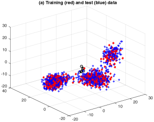
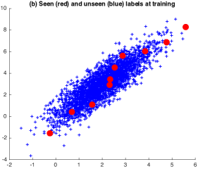
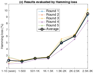
Figure 1: Synthetic data points (a), labels (b), and experimental results given different unseen labels (c). The data and labels used in training are in the red color. We evaluate the results of labeling the test data with the unseen labels by the Hamming loss. The performance decreases as the number of (Best viewed in color)

5 Empirical studies

In this section, we continue to investigate the properties of infinite-label learning. While the theoretical result in Section 4 justifies its learnability, there are many other questions of interest to explore for the practical use of the infinite-label learning. We focus on the following two questions and provide some empirical insights using respectively synthetic data and real data.

1. After we learn a decision function from the training set, how many and what types of unseen labels can we confidently handle using this decision function?

2. What is the effect of varying the number of seen labels $\mathcal{L}$, given a fixed union $\mathcal{L}\cup\mathcal{U}$ of seen and unseen labels? Namely, given a labeling task, can we collect training data for only a subset of the labels and yet achieve good performance at the test phase on all the labels? We learn different decision functions by varying the number of seen labels $\mathcal{L}$ and then check their labeling results of assigning all the labels $\mathcal{L}\cup\mathcal{U}$.

We use the bilinear form $h(\bm{x},\bm{\lambda})=\text{sgn}\left\langle V\bm{x},\bm{\lambda}\right\rangle$ for the decision function in the experiments, where our goal is not to achieve the state-of-the-art performance on the datasets but rather to demonstrate the feasibility of solving the infinite-label learning problems as well as revealing some trends and insights when the ratio between the numbers of seen and unseen labels changes.

5.1 Synthetic experiments

To answer the first question, we generate some synthetic data which allows us to conveniently control the number of labels for the experiments.

Data.

We randomly sample 500 training data points $\{\bm{x}_{m}\in\mathbb{R}^{3}\}_{m=1}^{\mathsf{M}=500}$ and 1000 testing data points from a five-component Gaussian mixture model. We also sample 10 seen labels $\mathcal{L}=\{\bm{\lambda}_{l}\in\mathbb{R}^{2}\}_{l=1}^{\mathsf{L}=10}$ and additionally 2990 unseen labels $\mathcal{U}=\{\bm{\lambda}_{11},\cdots,\bm{\lambda}_{3000}\}$ from a Gaussian distribution. Note that only the seen labels $\mathcal{L}$ are revealed during the training stage. As below specifies the distributions,

$$\bm{x} \sim P(\bm{x})=\sum_{k=1}^{5}\pi_{k}\,\mathcal{N}\left(\bm{\mu}_{k},\bm{U}_{k}\bm{U}_{k}^{T}\right),\quad\bm{x}\in\mathbb{R}^{3}$$

$$\bm{\lambda} \sim\mathcal{N}\left(\left[\begin{array}[]{c}2\\ 3\end{array}\right],\left[\begin{array}[]{cc}1&1.5\\ 1.5&3\end{array}\right]\right),\quad\bm{\lambda}\in\mathbb{R}^{2}$$

where the mixture weights $\pi_{k}$ are sampled from a Dirichlet distribution $\textsc{Dir}(3,3,3,3,3)$, and both the mean $\bm{\mu}_{k}$ and $\bm{U}_{k}$ for the variance are sampled from a standard normal distribution (using the randn function in MATLAB). Finally, we generate a “groundtruth” matrix $V\in\mathbb{R}^{2\times 3}$ from a standard normal distribution. The groundtruth label assignments are thus given by $y^{\star}_{ml}=\text{sgn}\left\langle V\bm{x}_{m},\bm{\lambda}_{l}\right\rangle$ for both training and testing data and both seen and unseen labels. Following Assumption II, we randomly flip the sign of each $y^{\star}_{ml}$ with probability $p=0.1$.

Figure 1(a) and (b) show the data points and labels we have sampled. The training data and the seen labels are in red color, while all the other (test) data points and labels are unseen during training. We choose the low dimensions for the data and vectorial labels so that we can visualize them and have a concrete understanding about the results to be produced.

Table 2: Comparison of different methods on the image tagging task when the number of seen tags varies.

Method    %	81 out of 81 tags are seen				73 out of 81 tags are seen				65 out of 81 tags are seen
	MiAP	P	R	F1	MiAP	P	R	F1	MiAP	P	R	F1
LabelEM [41]	47.4	26.2	44.7	33.1	41.8	23.4	39.8	29.4	38.4	21.4	36.4	26.9
ConSE [42]	47.5	26.5	44.9	33.2	46.9	26	44.3	32.7	44.9	24.3	41.5	30.7
ESZSL [7]	45.8	25.9	44.2	30.7	45.6	25.6	43.6	28.1	43.8	23.8	40.6	30.1
Bilinear-RankNet	53.8	30.1	51.4	38	52.8	29.5	50.2	37.1	49.5	27.5	46.8	34.6

Table 3: Continuation of Table 2, i.e., further comparisons of different methods on the image tagging task when the number of seen tags varies.

Method    %	57 out of 81 tags are seen				49 out of 81 tags are seen				41 out of 81 tags are seen
	MiAP	P	R	F1	MiAP	P	R	F1	MiAP	P	R	F1
LabelEM [41]	32.1	16.5	28.2	20.8	30.0	15.7	26.8	19.5	32.4	18.1	30.8	22.8
ConSE [42]	41.8	22.9	39.0	28.9	40.1	22.0	37.5	27.8	38.7	22.2	37.9	28.0
ESZSL [7]	41.6	22.8	38.9	28.7	39.6	21.7	36.9	27.3	38.4	21.9	37.4	27.6
Bilinear-RankNet	46.8	26.3	44.8	33.1	45.1	25.8	44.0	32.5	41.2	23.7	40.3	29.8

Algorithm.

Given the training set $\mathcal{S}$ of the 10 seen labels $\mathcal{L}$, we learn the labeling function $h(\bm{x},\bm{\lambda})=\text{sgn}\left\langle V\bm{x},\bm{\lambda}\right\rangle$ by minimizing a hinge loss,

$$\widehat{V}\leftarrow\arg\min_{V}\frac{1}{\mathsf{M}\mathsf{L}}\sum_{m=1}^{\mathsf{M}=500}\sum_{l=1}^{\mathsf{L}=10}\max\left(1-y_{ml}\left\langle V\bm{x}_{m},\bm{\lambda}_{l}\right\rangle,0\right),$$

and then try to assign both seen and unseen labels $\mathcal{L}\cup\mathcal{S}$ to the $1000$ test data points, using $\widehat{V}$. It is interesting to note that a similar formulation and its dual have been studied by Szedmak et al. [27], which, however, are mainly used to reduce the complexity of multi-class classification. It it also worth pointing out that it is not a regression problem though its form shares some similarity with the (multi-variate) support vector regression [43].

We incrementally challenge the learned infinite-label model $y_{ml}\leftarrow\text{sgn}\left\langle\widehat{V}\bm{x}_{m},\bm{\lambda}_{l}\right\rangle$ by gradually increasing the difficulties at the test phase. Namely, we rank all the labels according to their distances to the seen labels $\mathcal{L}$, where the distance between an unseen label $\bm{\lambda}_{l}$ and the seen ones $\mathcal{L}$ is calculated by $\min_{\bm{\lambda}\in\mathcal{L}}\|\bm{\lambda}-\bm{\lambda}_{l}\|_{2}$. We then evaluate the label assignment results for every 500 consecutive labels in the ranking list (as well as the 10 seen labels). Arguably, the last 500 labels, which are the furthest subset of unseen labels from the seen ones $\mathcal{L}$, impose the biggest challenge to the learned model.

Results.

Figure 1(c) shows the label assignment errors for different subsets of the test labels. We run 5 rounds of experiments each with different randomly sampled data, and report their individual results as well as the average. We borrow from multi-label classification [13] the Hamming loss as the evaluation metric. It is computed by $\frac{1}{1000}\sum_{m=1}^{1000}(|\bm{y}_{m}\neq\bm{y}^{\star}_{m}|^{T}\bm{1})/|\bm{y}^{\star}_{m}|^{T}\bm{1}$, where $\bm{y}^{\star}_{m}$ is the groundtruth label assignment to the data point $\bm{x}_{m}$ and $\bm{y}_{m}$ is the predicted assignment. Note that this is inherently different from the classification accuracy/error used for evaluating multi-class classification.

We draw the following observations from Figure 1(c). First, infinite-label learning is feasible since we have obtained decent results for up to 3000 labels with only 10 of them seen in training. Second, when the unseen labels are not far from the seen labels, the label assignment results are on par with the performance of assigning only the seen labels to the test data (cf. the Hamming losses over the first, second, and third 500 unseen labels). Third, labels that are far from the seen labels may cause larger confusions to the infinite-label model learned from finite seen labels. Increasing the number of seen labels and/or data points during training can improve the model’s generalization capability to unseen labels, as suggested by Theorem 1 and revealed in the next experiment.

Figure 2: The infinite-label learning results for image tagging under different numbers of seen labels.

5.2 Image tagging

We experiment with image tagging to seek some clues to answer the second question raised at the beginning of this section. Suppose we are given a limited budget and have to build a tagging model as good as possible under this budget. Thanks to the infinite-label learning, we may compile a training set using only a subset of the labels of interest as opposed to asking the annotators to examine all of them. Then, how many seen labels should we use in order to achieve about the same performance as using all of the labels for training? We give some empirical results to answer this question. Our experiment protocol largely follows the prior work [16].

Data.

We conduct the experiments using the NUS-WIDE dataset [39]. It has 269,648 images in total and we were only able to retrieve 223,821 of them using the provided image URLs. Among them, 134,281 are training images and the rest are testing images according to the official split by NUS-WIDE. We further randomly leave out 20% of the training images as the validation set for tuning hyper-parameters. The images are each represented by the are the $l_{2}$-normalized activations of the last fully connected layer of VGGNet-19 [44].

Each image in NUS-WIDE has been manually annotated with the relevant tags out of 81 candidate tags in total. We obtain the tags’ vectorial representations using the pre-trained GloVe word vectors [19]. While all the 81 tags are considered at the test stage, we randomly choose $\mathsf{L}=81$ (100% out of the 81 tags), 73 (90% out of the 81 tags), 65 (80% out of 81), 57 (70% out of 81), 49 (60% out of 81), and 41 (50% out of 81) seen tags for training different labeling functions $h(\bm{\lambda};\bm{x})=\text{sgn}\left\langle V\bm{x},\bm{\lambda}\right\rangle$. If a training image has no relevant tags under some of the settings, we simply drop it out of the training set.

Learning and evaluation.

Image tagging is often evaluated based on the top few tags returned by a system, assuming that users do not care about the remaining ones. We report the results measured by four popular metrics: Mean image Average Precision (MiAP) [45] and the top-3 precision, recall, and F1-score. Accordingly, in order to impose the ranking property to our labeling function, we learn it using the RankNet loss [46],

$$\widehat{V}\leftarrow\arg\min_{V}\frac{1}{\mathsf{M}}\sum_{m=1}^{\mathsf{M}}\frac{1}{(\mathsf{L}-{\mathsf{K}_{m}})\mathsf{K}_{m}}\sum_{\begin{subarray}{c}k:y_{mk}=+1\\ \bar{k}:y_{m\bar{k}}=-1\end{subarray}}$$

$$\log(1+\exp(\left\langle V\bm{x}_{m},\bm{\lambda}_{\bar{k}}\right\rangle-\left\langle V\bm{x}_{m},\bm{\lambda}_{k}\right\rangle))+\gamma\left\|V\right\|_{2},$$

where $\mathsf{K}_{m}$ is the number of relevant tags to the $m$-th image. The hyper-parameter $\gamma$ is tuned by the MiAP results on the validation set.

Baselines.

We compare our results to those of three state-of-the-art zero-shot learning methods: LabelEM [33] whose compatible function is the same as ours except that it learns the model parameters by structured SVM [41], ConSE [42] which estimates the representations of the unseen labels using the weighted combination of the seen ones’, and ESZSL [7] that enjoys a closed form solution thanks to the choice of the Frobenius norm.

The methods above were developed for multi-class classification, namely, to exclusively classify an image to one and only one of the classes. As a result, when we train them using the image tagging data, different tags may have duplicated images and result in conflict terms in the objective functions. We resolve this issue by removing such conflict terms in training. By doing this, we observe about 0.5%–2% absolute improvements for the baselines over blindly applying them to our infinite-label learning problem.

Results.

Tables 2 and 3 present the results of our method and the competitive baselines evaluated by the MiAP, top-3 precision, recall, and F1-score. We also plot the MiAPs and F1-scores in Figure 2 to visualize the differences between different methods and, more importantly, the changes over different numbers of seen labels. Recall that no matter how many labels are seen in the training set, the task remains the same at the test phase, i.e., to find all relevant labels from the 81 candidate tags for each image.

We can see that the performances of all the methods decrease as fewer seen tags are used for training. However, the performance drop is fairly gentle for our method—the MiAP drops by 1% (respectively, 3%) absolutely from using 100% seen labels for training to using 90% (respectively, from 90% to 80%). This confirms our conjecture that, with the semantic codes of the labels, we may save some human labor efforts for annotating the data without sacrificing the overall performance at the test phase.

Additionally, we find that our learned decision function outperforms all the competitive baseline methods by a large margin no matter under which experiment setting. This mainly attributes to that it is learned by a tailored loss function for the infinite-label learning problem, while the others are not at all. To some extent, such results affirm the significance of studying the infinite-label learning as a standalone problem because the existing methods for zero-shot classification are suboptimal for this new learning framework.

6 Conclusion

In this paper, we study a new machine learning framework, infinite-label learning. It fundamentally expands the scope of multi-label learning in the sense that the learned decision function can assign both seen and unseen labels to a data point from potentially an infinite number of candidate labels. We provide a formal treatment to the infinite-label learning, discuss its distinction from existing machine learning settings, lay out mild assumptions to a PAC-learning bound for the new problem, and also empirically examine its feasibilities and properties.

There are many potential avenues for the future work. Our current PAC bound can be likely improved and the assumptions could be relaxed. Theoretical understanding about its performance under the MiAP evaluation is also necessary given that MiAP is prevalent in evaluating the multi-label learning results, especially for image tagging. One particularly interesting application of the infinite-label learning is on the extreme multi-label classification problems [14]. We will explore them in the future work.

References

- [1] Hugo Larochelle, Dumitru Erhan, and Yoshua Bengio. Zero-data learning of new tasks. In AAAI, volume 1, page 3, 2008.
- [2] Mark Palatucci, Dean Pomerleau, Geoffrey E Hinton, and Tom M Mitchell. Zero-shot learning with semantic output codes. In Advances in neural information processing systems, pages 1410–1418, 2009.
- [3] Andrea Frome, Greg S Corrado, Jon Shlens, Samy Bengio, Jeff Dean, Tomas Mikolov, et al. Devise: A deep visual-semantic embedding model. In Advances in Neural Information Processing Systems, pages 2121–2129, 2013.
- [4] Richard Socher, Milind Ganjoo, Christopher D Manning, and Andrew Ng. Zero-shot learning through cross-modal transfer. In Advances in neural information processing systems, pages 935–943, 2013.
- [5] Christoph H Lampert, Hannes Nickisch, and Stefan Harmeling. Attribute-based classification for zero-shot visual object categorization. Pattern Analysis and Machine Intelligence, IEEE Transactions on, 36(3):453–465, 2014.
- [6] Jimmy Lei Ba, Kevin Swersky, Sanja Fidler, et al. Predicting deep zero-shot convolutional neural networks using textual descriptions. In Proceedings of the IEEE International Conference on Computer Vision, pages 4247–4255, 2015.
- [7] Bernardino Romera-Paredes and PHS Torr. An embarrassingly simple approach to zero-shot learning. In Proceedings of The 32nd International Conference on Machine Learning, pages 2152–2161, 2015.
- [8] Wei-Lun Chao, Soravit Changpinyo, Boqing Gong, and Fei Sha. An empirical study and analysis of generalized zero-shot learning for object recognition in the wild. In European Conference on Computer Vision, pages 52–68. Springer, 2016.
- [9] Yael Moses, Shimon Ullman, and Shimon Edelman. Generalization to novel images in upright and inverted faces. Perception, 25(4):443–461, 1996.
- [10] Peter JB Hancock, Vicki Bruce, and A Mike Burton. Recognition of unfamiliar faces. Trends in cognitive sciences, 4(9):330–337, 2000.
- [11] Andrew I Schein, Alexandrin Popescul, Lyle H Ungar, and David M Pennock. Methods and metrics for cold-start recommendations. In Proceedings of the 25th annual international ACM SIGIR conference on Research and development in information retrieval, pages 253–260. ACM, 2002.
- [12] Grigorios Tsoumakas, Ioannis Katakis, and Ioannis Vlahavas. Mining multi-label data. In Data mining and knowledge discovery handbook, pages 667–685. Springer, 2009.
- [13] Min-Ling Zhang and Zhi-Hua Zhou. A review on multi-label learning algorithms. Knowledge and Data Engineering, IEEE Transactions on, 26(8):1819–1837, 2014.
- [14] Kush Bhatia, Himanshu Jain, Purushottam Kar, Manik Varma, and Prateek Jain. Sparse local embeddings for extreme multi-label classification. In Advances in Neural Information Processing Systems, pages 730–738, 2015.
- [15] Jinseok Nam, Eneldo Loza Mencía, Hyunwoo J Kim, and Johannes Fürnkranz. Predicting unseen labels using label hierarchies in large-scale multi-label learning. In Joint European Conference on Machine Learning and Knowledge Discovery in Databases, pages 102–118. Springer, 2015.
- [16] Yang Zhang, Boqing Gong, and Mubarak Shah. Fast zero-shot image tagging. In The IEEE Conference on Computer Vision and Pattern Recognition (CVPR), June 2016.
- [17] Wei Bi and James Kwok. Efficient multi-label classification with many labels. In Proceedings of the 30th International Conference on Machine Learning (ICML-13), pages 405–413, 2013.
- [18] Tomas Mikolov, Ilya Sutskever, Kai Chen, Greg S Corrado, and Jeff Dean. Distributed representations of words and phrases and their compositionality. In Advances in neural information processing systems, pages 3111–3119, 2013.
- [19] Jeffrey Pennington, Richard Socher, and Christopher D Manning. Glove: Global vectors for word representation. In EMNLP, volume 14, pages 1532–1543, 2014.
- [20] Jason Weston, Samy Bengio, and Nicolas Usunier. Wsabie: Scaling up to large vocabulary image annotation. In IJCAI, volume 11, pages 2764–2770, 2011.
- [21] Alex Waibel. Modular construction of time-delay neural networks for speech recognition. Neural computation, 1(1):39–46, 1989.
- [22] Alireza Farhadi, Ian Endres, Derek Hoiem, and David Forsyth. Describing objects by their attributes. In Computer Vision and Pattern Recognition, 2009. CVPR 2009. IEEE Conference on, pages 1778–1785. IEEE, 2009.
- [23] Michiel Stock, Tapio Pahikkala, Antti Airola, Bernard De Baets, and Willem Waegeman. Efficient pairwise learning using kernel ridge regression: an exact two-step method. arXiv preprint arXiv:1606.04275, 2016.
- [24] Edwin V Bonilla, Felix V Agakov, and Christopher KI Williams. Kernel multi-task learning using task-specific features. In AISTATS, pages 43–50, 2007.
- [25] Bart Bakker and Tom Heskes. Task clustering and gating for bayesian multitask learning. Journal of Machine Learning Research, 4(May):83–99, 2003.
- [26] Kishan Wimalawarne, Masashi Sugiyama, and Ryota Tomioka. Multitask learning meets tensor factorization: task imputation via convex optimization. In Advances in neural information processing systems, pages 2825–2833, 2014.
- [27] Sandor Szedmak, John Shawe-Taylor, and Emilio Parado-Hernandez. Learning via linear operators: Maximum margin regression; multiclass and multiview learning at one-class complexity. University of Southampton, Tech. Rep, 2006.
- [28] Michiel Stock, Thomas Fober, Eyke Hüllermeier, Serghei Glinca, Gerhard Klebe, Tapio Pahikkala, Antti Airola, Bernard De Baets, and Willem Waegeman. Identification of functionally related enzymes by learning-to-rank methods. IEEE/ACM Transactions on Computational Biology and Bioinformatics (TCBB), 11(6):1157–1169, 2014.
- [29] Tapio Pahikkala, Antti Airola, Michiel Stock, Bernard De Baets, and Willem Waegeman. Efficient regularized least-squares algorithms for conditional ranking on relational data. Machine Learning, 93(2-3):321–356, 2013.
- [30] Ryan Prescott Adams, George E Dahl, and Iain Murray. Incorporating side information in probabilistic matrix factorization with gaussian processes. arXiv preprint arXiv:1003.4944, 2010.
- [31] Tinghui Zhou, Hanhuai Shan, Arindam Banerjee, and Guillermo Sapiro. Kernelized probabilistic matrix factorization: Exploiting graphs and side information. In Proceedings of the 2012 SIAM international Conference on Data mining, pages 403–414. SIAM, 2012.
- [32] Yi Fang and Luo Si. Matrix co-factorization for recommendation with rich side information and implicit feedback. In Proceedings of the 2nd International Workshop on Information Heterogeneity and Fusion in Recommender Systems, pages 65–69. ACM, 2011.
- [33] Zeynep Akata, Scott Reed, Daniel Walter, Honglak Lee, and Bernt Schiele. Evaluation of output embeddings for fine-grained image classification. In Proceedings of the IEEE Conference on Computer Vision and Pattern Recognition, pages 2927–2936, 2015.
- [34] Yanwei Fu, Yongxin Yang, Tim Hospedales, Tao Xiang, and Shaogang Gong. Transductive Multi-label Zero-shot Learning. pages 7.1–7.11. British Machine Vision Association, 2014.
- [35] Yongxin Yang and Timothy M Hospedales. A unified perspective on multi-domain and multi-task learning. arXiv preprint arXiv:1412.7489, 2014.
- [36] Daniel Hsu, Sham Kakade, John Langford, and Tong Zhang. Multi-label prediction via compressed sensing. In NIPS, volume 22, pages 772–780, 2009.
- [37] Yi Zhang and Jeff G Schneider. Multi-label output codes using canonical correlation analysis. In International Conference on Artificial Intelligence and Statistics, pages 873–882, 2011.
- [38] Krishnakumar Balasubramanian and Guy Lebanon. The landmark selection method for multiple output prediction. In Proceedings of the 29th International Conference on Machine Learning (ICML-12), pages 983–990, 2012.
- [39] Tat-Seng Chua, Jinhui Tang, Richang Hong, Haojie Li, Zhiping Luo, and Yantao Zheng. Nus-wide: a real-world web image database from national university of singapore. In Proceedings of the ACM international conference on image and video retrieval, page 48. ACM, 2009.
- [40] Mehryar Mohri, Afshin Rostamizadeh, and Ameet Talwalkar. Foundations of machine learning. MIT press, 2012.
- [41] Ioannis Tsochantaridis, Thorsten Joachims, Thomas Hofmann, and Yasemin Altun. Large margin methods for structured and interdependent output variables. Journal of machine learning research, 6(Sep):1453–1484, 2005.
- [42] Mohammad Norouzi, Tomas Mikolov, Samy Bengio, Yoram Singer, Jonathon Shlens, Andrea Frome, Greg S Corrado, and Jeffrey Dean. Zero-shot learning by convex combination of semantic embeddings. arXiv preprint arXiv:1312.5650, 2013.
- [43] Harris Drucker, Christopher JC Burges, Linda Kaufman, Alex Smola, Vladimir Vapnik, et al. Support vector regression machines. Advances in neural information processing systems, 9:155–161, 1997.
- [44] Karen Simonyan and Andrew Zisserman. Very deep convolutional networks for large-scale image recognition. arXiv preprint arXiv:1409.1556, 2014.
- [45] Xirong Li, Tiberio Uricchio, Lamberto Ballan, Marco Bertini, Cees GM Snoek, and Alberto Del Bimbo. Socializing the semantic gap: A comparative survey on image tag assignment, refinement and retrieval. arXiv preprint arXiv:1503.08248, 2015.
- [46] Chris Burges, Tal Shaked, Erin Renshaw, Ari Lazier, Matt Deeds, Nicole Hamilton, and Greg Hullender. Learning to rank using gradient descent. In Proceedings of the 22nd international conference on Machine learning, pages 89–96. ACM, 2005.