Measurements of Terahertz Radiation Generated using a Metallic, Corrugated Pipe

Abstract

A method for producing narrow-band THz radiation proposes passing an ultra-relativistic beam through a metallic pipe with small periodic corrugations. We present results of a measurement of such an arrangement at Brookhaven’s Accelerator Test Facility (ATF). Our pipe was copper and was 5 cm long; the aperture was cylindrically symmetric, with a 1 mm (radius) bore and a corrugation depth (peak-to-peak) of 60 um. In the experiment we measured both the effect on the beam of the structure wakefield and the spectral properties of the radiation excited by the beam. We began by injecting a relatively long beam compared to the wavelength of the radiation, but with short rise time, to excite the structure, and then used a downstream spectrometer to infer the radiation wavelength. This was followed by injecting a shorter bunch, and then using an interferometer (also downstream of the corrugated pipe) to measure the spectrum of the induced THz radiation. For the THz pulse we obtain and compare with calculations: the central frequency, the bandwidth, and the spectral power—compared to a diffraction radiation background signal.

Introduction

There is great interest in having a source of short, intense pulses of terahertz radiation. There are laser-based sources of such radiation, capable of generating few-cycle pulses with frequency over the range 0.5–6 THz and energy of up to 100  $\mu$J Lee05 . And there are beam-based sources, utilizing short, relativistic electron bunches. One beam-based method impinges an electron bunch on a thin metallic foil and generates coherent transition radiation (CTR). Recent tests of this method at the Linac Coherent Light Source (LCLS) have obtained single-cycle pulses of radiation that is broad-band, centered on 10 THz, and contains > 0.1 mJ of energy Daranciang:11 . Another beam-based method generates narrow-band THz radiation by passing a bunch through a metallic pipe coated with a thin dielectric layer Cook09 -Antipov12 .

Another, similar method for producing narrow-band THz radiation has proposed passing the beam through a metallic pipe with small periodic corrugations BaneStupakov_THz , which is the subject of the present report. We consider here round geometry which will yield radially polarized THz (studies of this idea in flat geometry can also be found Kim13 ). We present results of measurements of the spectral properties of the radiation excited by the beam.

A corrugated structure that we call “TPIPE" was tested with beam at the Accelerator Test Facility (ATF) at Brookhaven National Laboratory. We first used a relatively long beam, with short rise time—compared to the wavelength of the radiation—to excite the structure, and then used a downstream spectrometer to infer the central wavelength of the radiation. Then for a shorter bunch, by means of an interferometer also downstream of the corrugated pipe, we measured the spectrum of the induced THz. Due to a background of diffraction radiation of the bunch field, we could obtain the relative strength of the THz signal to this background. Our experimental set-up was simple and not optimized for the efficient collection of the radiation (by e.g. the inclusion of tapered horns between the structure and the collecting mirror of the interferometer, as was done in Refs. Andonian11 , Antipov12 ). As such, the present experiment should be considered a proof-of-principle experiment for generating THz using a round, corrugated, metallic structure.

Specifically, our goal in this work is to demonstrate a narrow-band THz signal downstream of TPIPE using the two measurement methods. In addition, we measure, and compare with calculations, the central frequency of the pulse, the bandwidth, and the relative strength of the signal at the central frequency.

Experimental Set-Up

A schematic of the experimental layout is presented in Fig. 1. A 57 MeV electron beam was initially shaped using a mask Muggli08 and then sent through TPIPE to generate a THz pulse. The beam leaves the structure directly followed by the THz pulse. At the exit of TPIPE the radiation pulse diffracts, and further downstream some of it is reflected by an off-axis parabolic mirror into a Michelson interferometer for characterization. The intensity of the THz signal collected is measured by an IRLabs General Purpose 4.2K (liquid helium) Bolometer System. Note that the mirror is located 17.5 cm beyond TPIPE, and that in front of the mirror is a 12.5 mm radius iris, which limits the radiation that is collected. As for the electron beam, it passes through a 2.5 mm radius hole in the mirror, where it generates diffraction radiation, some of which also ends up in the interferometer. Finally, the electron bunch enters the spectrometer for characterization.

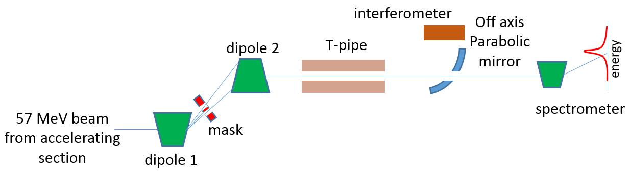
Figure 1: Sketch of the experimental layout.

To shape the beam we started by accelerating it off-crest in the accelerating section, in order to create a linear correlation between the longitudinal bunch coordinates $z$ and energy $E$. When the beam passes through a dipole magnet (“dipole 1" in Fig. 1) it becomes horizontally dispersed as in an energy spectrometer. A transverse mask is placed after the first dipole to block electrons of certain energies. A second dipole of opposing sign (“dipole 2") restores the beam to its original state, minus, however, the electrons that were blocked. Due to the $E$-$z$ correlation of the beam, the image in the downstream spectrometer also carries information about the beam’s longitudinal shape. Therefore, distances on the spectrometer image can be related to longitudinal distances within the beam.

Calculations

Central Frequency of THz Pulse

Consider a metallic beam pipe with a round bore and small, rectangular (in longitudinal view) corrugations (see Fig. 2). The parameters are period $p$, (full) depth of corrugation $\delta$, corrugation gap $g$, and pipe radius $a$; where we consider small corrugations ($\delta$, $p$) $\ll a$ and also $\delta\gtrsim p$. Let us here assume $p=2g$. It can be shown BaneStupakov_THz that a short, relativistic bunch, on passing through such a structure, will induce a wakefield that is composed of one dominant mode, of wave number $k\approx 2/\sqrt{a\delta}$, relative group velocity $v_{g}/c\approx 1-2\delta/a$, with $c$ the speed of light, and loss factor $\kappa\approx Z_{0}c/(2\pi a^{2})$, with $Z_{0}=377$ $\Omega$. In addition to the effect on the beam, a radiation pulse of the same frequency, with a uniform envelope (with a relatively sharp rise and fall) of full length $\ell=2\delta L/a$ ($L$ is pipe length) will follow the beam out the downstream end of the structure. One can see that, in order to generate a pulse of frequency $\sim 1$ THz, both the bore radius and the corrugation dimensions must be small; with $a\sim 1$ mm, then $\delta\lesssim 10$ $\mu$m. For $a=1$ mm, $\delta=60$ $\mu$m, the pulse frequency $f\approx 0.4$ THz. If, in addition, the pipe length is $L=5$ cm, then the full radiation pulse length, $\ell=6$ mm.

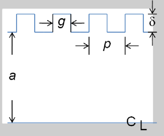
Figure 2: Idealized geometry of the corrugated structure. “CL" denotes the axis of the pipe.

TPIPE was machined from two rectangular blocks of high purity copper, each of dimension 2 cm by 1 cm by 5 cm on a side. Two 1-mm (radius) cylindrical grooves were first machined in the long direction in each block. One groove in each block was meant to remain smooth, for the null test of the experiment. The other groove was further machined, to give it corrugations. Originally, the goal was to have rectangular corrugations (in longitudinal view) with period $\sim 250$ $\mu$m and (total) depth of corrugation $\sim 60$ $\mu$m. However, rectangular corrugations of such small size are difficult to make; thus, a rounded profile was obtained using a 50 $\mu$m (radius) milling bit. When the machined blocks were measured at SLAC, it was determined that the corrugations actually had a period of $231$ $\mu$m and a depth of corrugation of 72 $\mu$m; furthermore, the radii of the “irises" and the “cavities" (in longitudinal view) were not identical, and were $r_{1}=91$ $\mu$m and $r_{2}=41$ $\mu$m, respectively (see Fig. 3, the blue curve). As the final step, the two copper blocks were diffusion bonded at SLAC to yield one block with two cylindrically symmetric bores, one corrugated and one smooth.

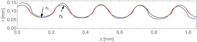
Figure 3: A rough digitization of the measured geometry of TPIPE’s corrugations (blue curve). The model used in ECHO simulations is also shown: arcs (brown curves) of radii $r_{1}=91$ $\mu$m and $r_{2}=41$ $\mu$m are connected by straight lines (in red), to give a structure with a period $p=231$ $\mu$m and a depth of corrugation of 72 $\mu$m.

We performed time-domain simulations with the 2D Maxwell equation solving program ECHO ECHO . We used a Gaussian bunch, with $\sigma_{z}=90$ $\mu$m, and let it pass through an entire 5-cm-long TPIPE structure. For the model used in the ECHO simulations, we used circular arcs (brown curves in Fig. 3) of radius $r_{1}=91$ $\mu$m and angular extent $\theta=\pi/2$ (for the irises), and of radius $r_{2}=41$ $\mu$m and angular extent $\theta=2\pi/3$ (for the cavities), and connected them by straight lines (in red). The final structure has period $p=231$ $\mu$m and a depth of corrugation of 72 $\mu$m. We see that the model gives a good approximation to the measured shape of TPIPE (the blue curve).

ECHO can calculate the wakefields that a Gaussian bunch excites when it passes through a vacuum chamber object. It can also monitor the electromagnetic fields that are excited as a function of time at a given location. In our simulations we monitored the fields at a fixed $z$ location at the downstream end of our model of TPIPE. In Fig. 4 (at the top) we show $E_{r}(t)$ ($t$ is time) at the monitor at $r=0.75$ mm. The bunch enters TPIPE (beginning at location $z=0$) at time $t=0$; it passes the monitor at $ct=z=5.15$ cm at the end of the structure. We see that the pulse begins with a relatively fast rise time followed by an oscillation with a uniform envelope. At the trailing end, however, there is a rather long tail. (In the same kind of calculation, for a different but similar corrugated structure, the tail is much less pronounced—see Fig. 5 in BaneStupakov_THz .) In the process of its generation, the THz pulse ends up long compared to the driving bunch because its group velocity ($v_{g}<c$) is less than the bunch velocity ($v\approx c$) BaneStupakov_THz ; the long tail of the THz pulse was thus generated near the entrance of the structure, and is apparently an initial transient effect. When it leaves the structure, the THz pulse has become $\ell\sim 5.8$ mm long (FWHM of envelope), consisting of $\sim 9$ oscillations.

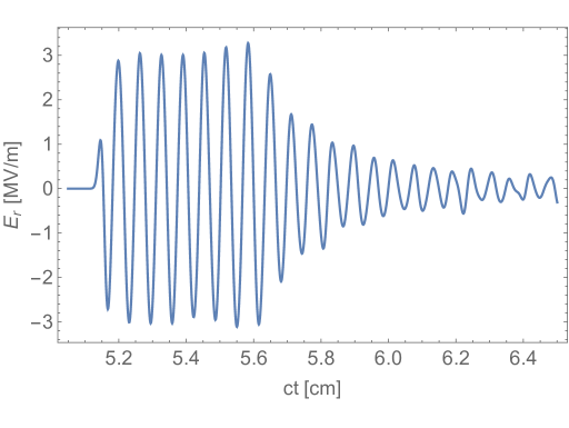
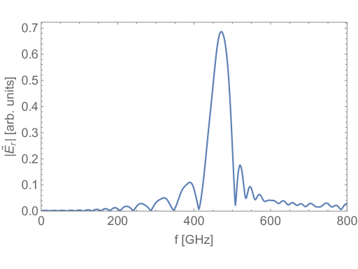
Figure 4: ECHO simulation results: The radial electric field $E_{r}$ at radius $r=0.75$ mm at a monitor located at the downstream end of TPIPE as function of time $t$ (top); here the driving bunch is Gaussian with $\sigma_{z}=90$ $\mu$m and charge $q=50$ pC. The absolute value of the Fourier transform of this function, $\tilde{E}_{r}$, as function of frequency $f$, is displayed at the bottom.

Performing the Fourier transform of $E_{r}$ and taking the absolute value, we obtain the spectrum of $|\tilde{E}_{r}|$, shown in Fig. 4 at the bottom. We see a clear, relatively narrow frequency spike, with central frequency $f_{c}=471$ GHz. For a $q=50$ pC bunch, the average energy loss is 13 keV (neglecting the loss at the entrance and exit planes of TPIPE), 90% of which (or 0.57 $\mu$J) ends up in the THz pulse, and 10% in Joule heating of the structure walls. According to ECHO, the spectral energy density (at the exit of TPIPE) at the central frequency is $(dU/df)_{\mathrm{T}}=0.0125$ $\mu$J/GHz.

Bandwidth of THz Pulse

The spectrum width of the THz pulse can be characterized by the quality factor $Q$ or, equivalently, relative bandwidth $\delta f$, where $Q\equiv 1/\delta f=f_{c}/\Delta f=8.3$ ($\Delta f$ is the full-width-at-half-maximum [FWHM] of the spectrum). (Note that the relative bandwidth in energy is approximately given by $\delta f/\sqrt{2}$.) There are two sources of the finite bandwidth of the pulse: a frequency variation within the pulse and the finite length of the pulse.

To estimate the effect of the finite pulse length we can start with an idealized model for the pulse field:

$$E_{r}(t)=E_{r0}H(t_{0}-t)H(t_{0}+t)\cos(2\pi f_{c}t)\ ,$$ (1)

where the peak field is $E_{r0}$, the unit step function, $H(x)=1$ (0) for $x>0$ ($<0$), a fixed frequency is $f_{c}$, and the parameter $t_{0}=n_{\lambda}/2f_{c}$, with $n_{\lambda}$ the number of oscillations in the pulse (an integer or half integer). Defining the Fourier transform by $\tilde{E}_{r}(f)=\int_{-\infty}^{\infty}E_{r}(t)e^{2\pi ift}dt$, we obtain

$$|\tilde{E}_{r}(f)|=\frac{E_{r0}}{\pi}\frac{f}{f^{2}-f_{c}^{2}}\left\{\begin{array}[]{r@{\quad:\quad}l}\sin(n_{\lambda}\pi f/f_{c})&n_{\lambda}{\rm\ integer}\\ \cos(n_{\lambda}\pi f/f_{c})&n_{\lambda}{\rm\ half\ integer}\end{array}\right.\ .$$ (2)

An idealized example of the pulse field, with $n_{\lambda}=9$, is shown in Fig. 5 (the left frame). In the right frame we display $|\tilde{E}_{r}(f)|$. The frequency of the peak divided by its FWHM defines the quality factor, $Q$. We find that, for this simple model, when $n_{\lambda}\gtrsim 3$, then $Q\approx n_{\lambda}/1.2$, which here equals 7.5.

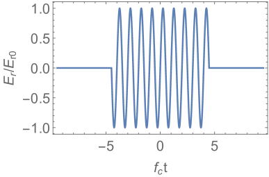
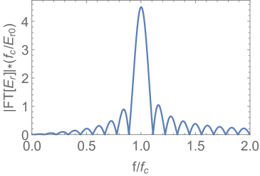
Figure 5: (Left) Idealized (model) pulse from a dechirper; (right) absolute value of Fourier transform of model pulse. The pulse contains $n_{\lambda}=9$ wavelengths; the resulting quality factor $Q=7.5\approx n_{\lambda}/1.2$.

Let us return to the ECHO calculation for TPIPE, where the $Q$ is obtained from the width (FWHM) of the spectrum peak in Fig. 4 (bottom plot), i.e. $Q=8.3$. From analyzing the ECHO data (Fig. 4, the top plot) we find that the effect on bandwidth of the frequency variation within the pulse is negligible compared to the effect of the finite length of the pulse. Thus, a measurement of the bandwidth can give us a reasonable estimate of the THz radiation pulse length

$$\ell=cn_{\lambda}/f_{c}\approx 1.2cQ/f_{c}\ .$$ (3)

With $Q=8.3$, this formula yields, $n_{\lambda}=10$ and $\ell=6.4$ mm, in reasonable agreement with the ECHO result of Fig. 4 (the top plot).

Relative Intensity of Signals Entering the Interferometer

When the beam leaves TPIPE, it is directly followed by the THz pulse. The THz pulse diffracts at the exit of TPIPE and propagates downstream, where some of it is intercepted by the mirror and enters the interferometer. As for the beam, as it reaches the mirror and passes through a hole in it, it generates a diffraction radiation pulse—sometimes called a coherent transition radiation (COTR) pulse; some of this pulse is also captured by the interferometer. Here we endeavor to calculate: (1) the fraction of THz pulse that reaches the mirror and (2) the amount of diffraction radiation that is generated by the beam at the mirror.

Note that if there are two sources of radiation, their fields or impedances just add, from the principle of linear superposition of fields. Their power spectra, however, can interfere. We assume here that the power spectra of the THz signal and diffraction radiation background just add. This is true in our case, to good approximation, since the two sources of radiation are (mostly) separated in time: the THz pulse follows right behind the bunch, where the full bunch length is $\sim 2\sigma_{z}\sim 200$ $\mu$m, whereas the THz pulse length is $\sim 6$ mm long.

As mentioned above, ECHO found that, at the exit of TPIPE, the spectral power in the THz pulse, at the central frequency (471 GHz), is $(dU/df)_{\mathrm{T}}=0.0125$ $\mu$J/GHz. The THz pulse diffracts when it leaves TPIPE. In Appendix A we derive an expression that can be used to find the fraction of spectral power in the pulse that reaches the mirror downstream (see Eq. 23):

$$\rho_{\mathrm{THz}}=F\left(\frac{kab}{L}\right)\ ,$$ (4)

$$F(x)=1-\left(\frac{4}{x^{2}}+2\right)J_{1}(x){}^{2}-2J_{0}(x){}^{2}+\frac{4}{x}J_{1}(x)J_{0}(x)\ ,$$ (5)

with $k=2\pi f/c$ the wave number, $a$ the radius of the corrugated pipe, $b$ the radius of the mirror, $L$ the distance between the end of the corrugated pipe and the mirror, and $J_{0}(x)$, $J_{1}(x)$, are Bessel functions of the first kind.

For the parameters of the experiment (see Table 1) and central frequency (according to ECHO) $f=ck/2\pi=471$ GHz, we find that the fraction of THz pulse energy that reaches the mirror is

$$\rho_{\mathrm{THz}}=3.6\times 10^{-3}\ .$$ (6)

Table 1: Parameters used in the analysis of the interferometry measurements.

Parameter	Value	Unit
Energy, $E$	57.	MeV
TPIPE bore radius, $a$	1.0	mm
Distance to mirror, $L$	17.5	cm
Mirror radius, $b$	12.5	mm
Mirror hole radius, $b_{1}$	2.5	mm

In Appendix B we derive the spectral power in the diffraction radiation pulse, generated when the beam passes through the hole in the mirror. The result is (30)

$$\left(\frac{dU}{df}\right)_{\mathrm{d}}=\frac{4q^{2}|\tilde{\lambda}(k)|^{2}}{c}\left[G\left(\frac{kb}{\gamma}\right)-G\left(\frac{kb_{1}}{\gamma}\right)\right]\ ,$$ (7)

$$G(x)=\frac{1}{2}x^{2}\left[K_{1}(x){}^{2}-K_{0}(x)K_{2}(x)\right]\ ,$$ (8)

with $q$ bunch charge, $\tilde{\lambda}(k)$ the Fourier Transform of the bunch distribution, $b$ radius of the mirror, $b_{1}$ radius of the hole in the mirror, $\gamma$ Lorentz energy factor, and $K_{0}(x)$, $K_{1}(x)$, modified Bessel functions of the second kind. For a Gaussian bunch $|\tilde{\lambda}(k)|^{2}=e^{-k^{2}\sigma_{z}^{2}}$. Substituting into Eq. 7 the parameters of Table 1 and: $q=50$ pC, $k=2\pi f_{c}/c=9.9$ mm^-1 ($f_{c}=471$ GHz), $\gamma=120$, and $\sigma_{z}=90$ $\mu$m, we obtain

$$\left(\frac{dU}{df}\right)_{\mathrm{d}}=1.5\times 10^{-4}\,\,\mu\textrm{J/GHz}.$$ (9)

Finally, at the mirror, at frequency $f=471$ GHz, the ratio of the spectral power in the THz pulse to that in the diffraction radiation pulse is

$$\Lambda\equiv\rho_{\mathrm{THz}}\left(\frac{dU}{df}\right)_{\mathrm{T}}\Bigg{/}\left(\frac{dU}{df}\right)_{\mathrm{d}}=0.30\ .$$ (10)

Note that, because the comparison of the spectral power of the two sources is done at one frequency, where the excitation of both signal and background depend on $|\tilde{\lambda}(k)|^{2}$, the final result is relatively insensitive to bunch length.

Below we will compare these results with interferometer measurements. We have made simplifying assumptions. We have calculated the relative spectral power at the mirror, assuming the mirror is flat and perpendicular to the beam trajectory; in reality the mirror is parabolic and tilted at an angle. We have also assumed that the THz signal and diffraction radiation background add in the energy spectrum, but there will be some interference—though we believe it to be small.

Results

Spectrometer Measurements

If we pass a long bunch with a short rise time—both compared to TPIPE’s wavelength—through the structure, the beam will become energy modulated at the structure frequency (see e.g. Antipov13 ). If the long bunch has an energy chirp, then the wavelength of the mode can be measured on the spectrometer screen. In Fig. 6 we compare the energy spectrum measurements of: the original beam, with TPIPE removed from its path (a), the beam passing through the corrugated pipe in TPIPE (b), and the beam passing through the smooth tube in TPIPE (c). The green line gives the energy distribution of case (a), the red line that of case (b). First, we note that the results for the cases of no TPIPE and the smooth pipe are similar, showing a chirped streak with no modulation. With the corrugated pipe (b) we see a clear modulation. The bunch length was measured by coherent transition radiation interferometry Muggli08 . Based on the spacing of the energy modulation and the bunch length to energy chirp calibration, we estimate that the frequency of the TPIPE mode is ($459\pm 32$) GHz, taking into account the resolution of the energy spectrometer and the uncorrelated beam energy spread. From the energy modulation measurement we estimate the maximum decelerating field inside the long bunch is ($1\pm 0.2$) MV/m. This field value is a measure of the bunch current rise time.

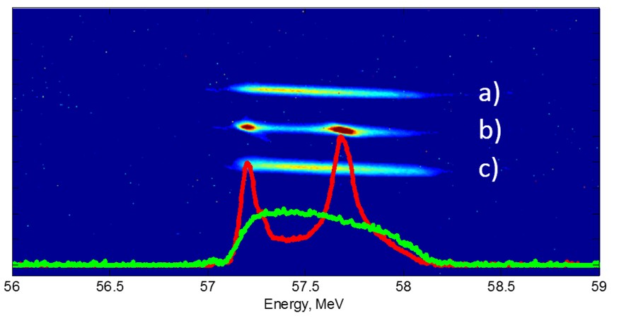
Figure 6: Spectrometer images: no structure (a), TPIPE (b), smooth pipe (c). In all cases the beam is initially chirped, resulting in a horizontal streak on the screen. The green line gives the energy distribution of case (a), the red line that of case (b).

Interferometer Measurements

For the interferometer scans we need a shorter bunch, generated using a mask, as described above. A 22-mm-long interferometer scan (with a 20 $\mu$m step size), with the beam passing through TPIPE, is shown in Fig. 7 in the left plot, where $ct$ gives the path length change in the light in one arm of the interferometer, equal to twice the distance of travel of the movable mirror in the interferometer (both with arbitrary offset). This plot is actually the composite of three scans, where we verified that the oscillations at the boundaries (of the three scans) matched well in amplitude and phase of oscillation. The bunch charge was $q=50$ pC. The right plot in Fig. 7 zooms in to show more details of the central portion of the scan.

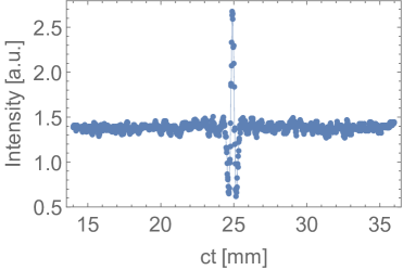
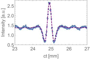
Figure 7: (Left frame) A fine, 22-mm interferometer scan of the radiation generated by TPIPE; $ct$ is path length change of the light in one arm of the interferometer (with arbitrary offset). The data points (the symbols) are connected by straight lines to aid the eye. (Right frame) A zoomed-in shot of the center of the scan. Here the purple, dashed curve gives the best fit to the diffraction radiation model for a Gaussian beam, discussed below.

After padding with zeros, a Fast Fourier Transform (FFT) of the scan of Fig. 7 (on the left) was performed. The absolute value of the Fourier transform is given in Fig. 8. We see a rather broad peak topped by a narrow horn. We consider this spectrum to be the sum of the spectra of: the narrow-band THz pulse generated at TPIPE (the signal), and the broad-band, diffraction radiation pulse generated at the mirror (the background).

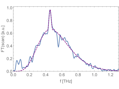
Figure 8: The absolute value of the Fourier transform of the scan of Fig. 7 (the blue, solid curve). The dashed, purple curve gives the best model fit.

The broad spectrum that is recorded has a low frequency cut-off given by the apertures in the interferometer, and a high frequency cut-off determined by the bunch spectrum. There are features in the plot that are not understood and that we consider artifacts, such as a peak near $f=100$ GHz and some ripples in the spectrum. In our experiment, no measures were taken to keep water vapor out of the interferometer, and prominent dips seen in the spectrum at $f=557.1$ GHz, 750.5 GHz, closely match the first two absorption frequencies of water vapor, 557. GHz and 752. GHz (see e.g. Slocum ; these dips were found in all our scans). These dips can serve as indications of the accuracy of the frequency values in the plot.

To approximate the broad, diffraction radiation background we choose the function Leissner99

$$\tilde{S}(k,\sigma_{z},\zeta)=e^{-k^{2}\sigma_{z}^{2}}(1-e^{-k^{2}\zeta^{2}})^{2}\ ,$$ (11)

with the two fitting parameters bunch length $\sigma_{z}$ and $\zeta$; the high frequency behavior is that generated by a Gaussian bunch with rms length $\sigma_{z}$. Note that, in the time domain, this function becomes Leissner99

$$S(s,\sigma_{z},\zeta)=\left(e^{-\frac{z^{2}}{4/\sigma_{z}^{2}}}-\frac{2\sigma_{z}\cdot e^{-\frac{s^{2}}{4(\sigma_{z}^{2}+\zeta^{2})}}}{\sqrt{\sigma_{z}^{2}+\zeta^{2}}}+\frac{\sigma_{z}\cdot e^{-\frac{s^{2}}{4(\sigma_{z}^{2}+2\zeta^{2})}}}{\sqrt{\sigma_{z}^{2}+2\zeta^{2}}}\right)\ ,$$ (12)

with $s=ct$.

As our model spectrum function, we take the sum of the diffraction radiation background (Eq. 11) and the model of the THz signal ($|\tilde{E}_{r}|^{2}$ taken from Eq. 2); specifically, we take intensity to be given by

$$I(f)=\alpha_{1}{\tilde{S}}(2\pi f/c,\sigma_{z},\zeta)+\alpha_{2}|\tilde{E}_{r}(f,f_{c},n_{\lambda})/E_{r0}|^{2}\ ,$$ (13)

with fitting parameters $\alpha_{1}$, $\sigma_{z}$, $\zeta$, for the broad-band diffraction radiation background, and $\alpha_{2}$, $f_{c}$, $n_{\lambda}$, for the narrow-band THz signal. Before fitting to the spectrum of Fig. 8, we remove the artificial peak near $f=100$ GHz and the dip due to water vapor at $f=557$ GHz. We fit using the Maximum-Likelihood Method (see e.g. BevingtonRobinson ), where it is assumed that the measured values of $I(f)$ have independent, normally distributed errors. This method, in addition to finding the best fitting parameters, gives us also an estimate of their errors.

The best fit is shown by the dashed, purple curve in Fig. 8. We see that the fit is indeed good. For the parameters connected to diffraction radiation, we find that the fitted $\sigma_{z}=(87.\pm 1)$ $\mu$m and $\zeta=(137.\pm 2)$ $\mu$m. That the fit is quite good at the higher frequencies indicates that a Gaussian bunch of $\sigma_{z}=87$ $\mu$m gives a reasonable approximation to the bunch shape. In the time domain, the fitted filter function, Eq. 12, also matches the central part of the data well (see Fig. 7 on the right, the purple dashed curve).

The narrow peak in the spectrum of Fig. 8, corresponding to the THz signal, is also fit well by the model. The relevant fitted parameters are: $f_{c}=(454.2\pm 0.6)$ GHz and $n_{\lambda}=13\pm\frac{1}{2}$. The fitted parameters imply (see Eq. 3): the quality factor, $Q=10.8\pm 0.4$, and the pulse length, $\ell=(8.6\pm 0.3)$ mm. The central frequency agrees with the spectrometer measurement discussed above and (reasonably well) with the ECHO calculations (471 GHz). The 4% disagreement with the calculations suggests that there is still some error in our understanding of the shape of the corrugations.

As for the $Q$, note that there is a maximum value of $Q$ that can be resolved from an interferometer scan. An interferometer scan, in essence, is the result—after high-pass filtering of the radiation pulse—of performing an autocorrelation. For a pulse of finite length, the autocorrelation will have double that length. The interferometer scans will have a finite total difference in path length of the light; let us denote it by $\Delta ct$. From the discussion in the “Bandwidth of THz Pulse" section above and from Eq. 3, we find that for given $\Delta ct$, the maximum quality factor that can be resolved is

$$Q_{max}=\frac{f_{c}\Delta ct}{2.4c}\ .$$ (14)

Here $Q_{max}=14$; thus, it appears that our fitted $Q$ (10.8) is not limited by the resolution of the measurement.

The measured ratio, at $f_{c}=454$ GHz, of the spectral power of the THz signal to that of the diffraction radiation background is $\Lambda=0.50\pm 0.05$. The calculated result, given above ($\Lambda=0.30$), is only 60% of this value, suggesting that the amount of diffraction radiation that was recorded is less than expected. We originally thought that one reason this might be is that—between the exit of TPIPE and the location of the mirror—the beam’s primary fields have not had a chance to reconstitute themselves; a simulation with ECHO, however, ruled out this as a significant effect here. Another possible reason for a disagreement in the diffraction radiation may be due to the fact that the mirror geometry is not simply a flat, round disc orientated perpendicular to the beam trajectory; this could be verified by e.g. performing a 3D ECHO simulation with the real geometry. Nevertheless, given the simplicity of the model in the calculations, we believe that an agreement to 60% represents reasonably good agreement. A summary of the main results obtained from the spectrum of Fig. 8 can be found in Table 2.

Table 2: Summary of main results obtained from interferometry: properties of the THz pulse, comparing calculations with analysis of the scan of Fig. 7. Note that the experimental value of pulse length $\ell$ is estimated from the measured quality factor $Q$ according to Eq. 3.

Parameter	Theory	Experiment	Units
Central frequency, $f_{c}$	471.	454.2	GHz
Quality factor, $Q$	8.3	10.8
Pulse length (FWHM), $\ell$	5.8	8.6	mm
Relative strength, $(dU/df)$, at $f=f_{c}$, $\Lambda$	0.30	0.50

For the null test, we present in Figs. 9–10, interferometer results for the case of the beam passing through the smooth tube in TPIPE, and the case TPIPE is withdrawn completely from the path of the beam (left plots gives the scan, the right ones the Fourier transform). These scans were performed one after the other late in the data taking, when the helium was nearly depleted; this fact resulted in a much weaker signal and probably accounts for the larger number of artifacts (oscillations) seen in the spectrum (especially the smooth pipe case). In addition, the scans only included a total path length difference, $\Delta ct=8$ mm, reducing the resolution in frequency. We again see the dips near $f=555$ GHz, 750 GHz, but this time there is no clear horn or signal on top that can be identified as a narrow-band THz signal. The spectra, in both cases, are essentially the same. The dashed, purple curve in the plots give the fit to the function, Eq. 11; in Fig. 9 with $\sigma_{z}=68$ $\mu$m and $\zeta=155$ $\mu$m; in Fig. 10 with $\sigma_{z}=74$ $\mu$m and $\zeta=153$ $\mu$m.

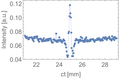
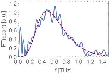
Figure 9: Interferometry scan and spectrum for the case of the beam passing through the smooth bore of TPIPE.

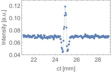
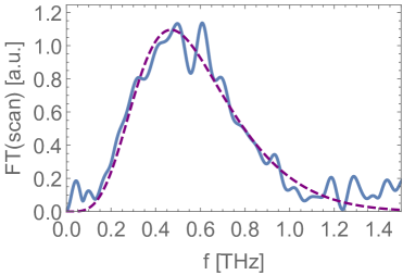
Figure 10: Interferometry scan and spectrum for the case of TPIPE withdrawn from the path of the beam.

We had more interferometer scans with TPIPE, and for different bunch lengths. However, many were of poor quality, and most were for total scan length $\Delta ct=4$ mm, where there is insufficient resolution for obtaining $f_{c}$ or $\Lambda$, and certainly not for $Q$. One good measurement with $\Delta ct=8$ mm yielded a spectral peak at $f_{c}=456.2$ GHz, in reasonable agreement with the value of 454.2 GHz obtained by our best scan, presented in detail above.

Conclusions

We have demonstrated the generation of a narrow-band THz pulse by having a relativistic beam pass through a round, corrugated metallic pipe by two methods: (1) using a relatively long bunch (with short rise time) to energy modulate the beam, that—after introducing an energy chirp—was detected in a spectrometer; (2) using a short bunch to generate a narrow-band THz pulse that was detected using an interferometer and a LHe bolometer. The null cases—those of a smooth pipe or with the corrugated structure completely removed from the beam path—found no narrow-band signal.

In addition to this proof-of-principle demonstration, we measured (and compared with calculations): the central frequency of the pulse, $f_{c}=454$ GHz, the effective quality factor $Q=10.8$, and the relative strength of the signal at the central frequency (to a diffraction radiation background), $\Lambda=0.50$. These results are all in reasonable agreement with our calculations. From the $Q$ value, we can estimate the THz pulse full length to be $\ell=8.6$ mm.

We have only one good measurement of TPIPE with the interferometer, and thus have no good estimate of the experimental errors. Considering the central frequency $f_{c}$, for example, one can conservatively take the error estimate to be $c/\Delta ct=15$ GHz ($\Delta ct$ is the full scan range of path length difference). However, comparing prominent dips in the spectrum to the first two absorption lines of water vapor and finding differences $\leq 1.5$ GHz, suggest that the accuracy is much better.

Appendix A Fraction of THz Energy that Reaches the Mirror

We compute here the relative loss of spectral power in the THz pulse—between the exit of the corrugated structure and the arrival at the mirror—due to diffraction of the wave. The electric field at the exit of the corrugated pipe is approximated by

$$\textnormal{\boldmath$\mathcal{E}$}(\textnormal{\boldmath$r$})=A{\textnormal{\boldmath$r$}}e^{-2\pi ift}\ ,$$ (15)

with $A$ a constant, $r$ is the transverse position, $f$ is the frequency, and $t$ is time. (We will drop the $e^{-2\pi ift}$ in the following equations; this factor does not affect spectral energy results.) The spectral energy of this field

$$W=\frac{1}{4\pi}\int 2\pi rdr\,|\textnormal{\boldmath$\mathcal{E}$}(\textnormal{\boldmath$r$})|^{2}=\frac{1}{2}A^{2}\int_{0}^{a}r^{3}dr=\frac{1}{8}A^{2}a^{4}\ ,$$ (16)

where $a$ is the radius of the corrugated pipe.

To find the distribution of the electric field at the downstream mirror, $\textnormal{\boldmath$E$}_{\mathrm{m}}(\textnormal{\boldmath$r$}^{\prime})$, we use vectorial diffraction theory Jackson

$${{\textnormal{\boldmath$E$}}}_{\mathrm{m}}(\textnormal{\boldmath$r$}^{\prime})=-e^{ikL+ik{r^{\prime}}^{2}/2L}\frac{ik}{2\pi L}\int e^{{-ik\textnormal{\boldmath$r^{\prime}$}\cdot\textnormal{\boldmath$r$}/L}}\textnormal{\boldmath$\mathcal{E}$}(\textnormal{\boldmath$r$})\,d^{2}r\ ,$$ (17)

where $k=2\pi f/c$, $L$ is the distance between corrugated pipe and mirror, and the integral is performed over the cross-section of the pipe. It is clear that $\textnormal{\boldmath$E$}_{\mathrm{m}}$ is directed along $\textnormal{\boldmath$r$}^{\prime}$; i.e. ${{\textnormal{\boldmath$E$}}}_{\mathrm{m}}(\textnormal{\boldmath$r$}^{\prime})=E_{\mathrm{m}}(r^{\prime})\textnormal{\boldmath$r$}^{\prime}/r^{\prime}$. For $E_{\mathrm{m}}$ we obtain

$$E_{\mathrm{m}} =e^{ikL+ik{r^{\prime}}^{2}/2L}\frac{ik}{2\pi L}A\int d^{2}r\,e^{{-ik\textnormal{\boldmath$r^{\prime}$}\cdot\textnormal{\boldmath$r$}/L}}\textnormal{\boldmath$r$}\cdot\frac{\textnormal{\boldmath$r$}^{\prime}}{r^{\prime}}$$

$$=e^{ikL+ik{r^{\prime}}^{2}/2L}\frac{ik}{2\pi L}A\int_{0}^{\infty}r^{2}dr\int_{0}^{2\pi}d\phi\,e^{{-ik{r^{\prime}}{r}\cos\phi/L}}\cos\phi\ .$$ (18)

The integral over $\phi$ can be taken using

$$\int_{0}^{2\pi}e^{-i\alpha\cos\phi}\cos\phi\,d\phi=-2\pi iJ_{1}(\alpha)\ ,$$ (19)

with the result

$$E_{\mathrm{m}} =e^{ikL+ik{r^{\prime}}^{2}/2L}\frac{k}{L}A\int_{0}^{a}r^{2}dr\,J_{1}\left(\frac{k{r^{\prime}}{r}}{L}\right)$$

$$=e^{ikL+ik{r^{\prime}}^{2}/2L}A\frac{a^{2}}{r^{\prime}}J_{2}\left(\frac{k{r^{\prime}}a}{L}\right).$$ (20)

We compute the spectral energy reaching the mirror by using (16) with the electric field at the mirror (A)

$$W_{\mathrm{m}} =\frac{1}{4\pi}\int_{0}^{b}2\pi r^{\prime}dr^{\prime}|E_{\mathrm{m}}(r^{\prime})|^{2}=\frac{1}{2}A^{2}a^{4}\int_{0}^{b}\frac{dr^{\prime}}{r^{\prime}}J_{2}^{2}\left(\frac{k{r^{\prime}}a}{L}\right)$$

$$=\frac{1}{8}A^{2}a^{4}F\left(\frac{kab}{L}\right),$$ (21)

where $b$ is the mirror radius and

$$F(x)=1-\left(\frac{4}{x^{2}}+2\right)J_{1}(x){}^{2}-2J_{0}(x){}^{2}+\frac{4}{x}J_{1}(x)J_{0}(x)\ .$$ (22)

Finally, the ratio of the THz spectral power that arrives at the mirror to that at the exit of the corrugated pipe is

$$\rho_{\mathrm{THz}}\equiv\frac{W_{\mathrm{m}}}{W}=F\left(\frac{kab}{L}\right)\ .$$ (23)

Appendix B Diffraction Radiation Background

An ultra-relativistic beam passes through a hole in a mirror. The electromagnetic energy hitting the mirror can be written in terms of the radial electric field $E(r,z)$ as

$$U=\frac{1}{4\pi}\int_{-\infty}^{\infty}dz\int_{b_{1}}^{b}2\pi rdr\,E(r,z)^{2}\ ,$$ (24)

(we took into account that the magnetic field is equal to the electric one). The lower limit $b_{1}$ is the radius of the hole in the mirror. If the bunch longitudinal distribution function $\lambda(z)$ is normalized to unity, then $E(r,z)$ can be computed as a superposition of the field of a point charge $E_{p}(r,z)$:

$$E(r,z)=q\int dz^{\prime}\lambda(z^{\prime})E_{p}(r,z-z^{\prime})\ ,$$ (25)

where $q$ is the total charge of the beam.

Fourier transforming (25), we find

$$\tilde{E}(r,k)=\int_{-\infty}^{\infty}dz\,e^{-ikz}E(r,z)=q\tilde{\lambda}(k)\tilde{E}_{p}(r,k)\ .$$ (26)

From the Parseval’s theorem

$$\int_{-\infty}^{\infty}dz\,E(r,z)^{2}=\frac{1}{\pi}\int_{0}^{\infty}dk\,|\tilde{E}(r,k)|^{2}\ ;$$ (27)

hence the spectral energy (with dimensions J/Hz)

$$\left(\frac{dU}{df}\right)_{\mathrm{d}}=\frac{1}{c}\int_{b_{1}}^{b}rdr\,|\tilde{E}(r,k)|^{2}=\frac{q^{2}|\tilde{\lambda}(k)|^{2}}{c}\int_{b_{1}}^{b}rdr\,|\tilde{E}_{p}(r,k)|^{2},$$ (28)

where $f=ck/2\pi$. The Fourier transform of the field of a relativistic point charge is well known,

$$|\tilde{E}_{p}(r,k)|=\frac{2k}{\gamma}K_{1}\left(\frac{kr}{\gamma}\right)\ .$$ (29)

Thus, we obtain

$$\left(\frac{dU}{df}\right)_{\mathrm{d}}=\frac{4q^{2}|\tilde{\lambda}(k)|^{2}}{c}\int_{b_{1}}^{b}rdr\frac{k^{2}}{\gamma^{2}}K_{1}\left(\frac{kr}{\gamma}\right)^{2}=\frac{4q^{2}|\tilde{\lambda}(k)|^{2}}{c}\left[G\left(\frac{kb}{\gamma}\right)-G\left(\frac{kb_{1}}{\gamma}\right)\right]\ ,$$ (30)

with

$$G(x)=\frac{1}{2}x^{2}\left[K_{1}(x){}^{2}-K_{0}(x)K_{2}(x)\right].$$ (31)

References

- (1) Y.-S. Lee et al, “Multi-cycle THz pulse generation in poled lithium niobate crystals," Laser Focus World 2005, 67 (2005).
- (2) D. Daranciang et al, “Single-cycle terahertz pulses with >0.2 V/Å field amplitudes via coherent transition radiation," Appl. Phys. Lett. 99, 141117 (2011).
- (3) A.M. Cook et al, “Observation of Narrow-Band Terahertz Coherent Cherenkov Radiation from a Cylindrical Dielectric-Lined Waveguide," Phys. Rev. Lett. 103, 095003 (2009).
- (4) G. Andonian et al, “Resonant excitation of coherent Cerenkov radiation in dielectric lined waveguides," Appl. Phys. Lett. 98, 202901 (2011).
- (5) S. Antipov et al, “Experimental demonstration of wakefield effects in a THz planar diamond accelerating structure," Appl. Phys. Lett. 100, 132910 (2012).
- (6) K. Bane and G. Stupakov, “Terahertz Radiation from a Pipe with Small Corrugations," Nucl. Instrum. Meth. A 677, 67 (2012).
- (7) Y. Kim et al, Proc. of PAC2013, “Demonstration of a Compact High Average Power THz Light Source at the IAC," Pasadena, CA, 2013, p. 282–204.
- (8) I. Zagorodnov and T. Weiland, “TE/TM field solver for particle beam simulations without numerical Cherenkov radiation," Phys. Rev. ST Accel. Beams 8, 042001 (2005).
- (9) P. Muggli et al, “Generation of Trains of Electron Microbunches with Adjustable Subpicosecond Spacing," Phys. Rev. Lett. 101, 054801 (2008).
- (10) S. Antipov et al, “Subpicosecond Bunch Train Production for a Tunable mJ Level THz Source," Phys. Rev. Lett. 111, 134802 (2013).
- (11) D.M. Slocum et al, “Atmospheric absorption of terahertz radiation and water vapor continuum effects," J Quant. Spectrosc. Radiat. Transfer (2013), http://dx.doi.org/10.1016/j.jqsrt.2013.04.022.
- (12) B. Leissner et al, “Bunch Length Measurements using a Martin Puplett Interferometer at the TESLA Test Facility Linac," Proc. of the 1999 PAC, New York, NY, 1999, p. 2172–2174.
- (13) J.D. Jackson, Classical Electrodynamics, 2nd Edition (John Wiley & Sons, New York, 1975) pp. 435ff.
- (14) P.R. Bevington and D.K. Robinson, Data Reduction and Error Analysis for the Physical Sciences, 2nd Edition (McGraw-Hill, Inc., New York, 1992) Chap. 10.