Event-driven Trajectory Optimization for Data Harvesting in Multi-Agent Systems

Abstract

We propose a new event-driven method for on-line trajectory optimization to solve the data harvesting problem: in a two-dimensional mission space, $N$ mobile agents are tasked with the collection of data generated at $M$ stationary sources and delivery to a base with the goal of minimizing expected collection and delivery delays. We define a new performance measure that addresses the event excitation problem in event-driven controllers and formulate an optimal control problem. The solution of this problem provides some insights on its structure, but it is computationally intractable, especially in the case where the data generating processes are stochastic. We propose an agent trajectory parameterization in terms of general function families which can be subsequently optimized on line through the use of Infinitesimal Perturbation Analysis (IPA). Properties of the solutions are identified, including robustness with respect to the stochastic data generation process and scalability in the size of the event set characterizing the underlying hybrid dynamical system. Explicit results are provided for the case of elliptical and Fourier series trajectories and comparisons with a state-of-the-art graph-based algorithm are given.

I Introduction

Systems consisting of cooperating mobile agents have been extensively studied and used in a broad spectrum of applications such as environmental sampling [1],[2], surveillance [3], coverage [4],[5],[6], persistent monitoring [7],[8], task assignment [9], and data harvesting and information collection [10],[11],[12].

The data harvesting problem in particular (and its variant, the “minimum latency” problem [13]) arises in many settings where wireless sensor networks (WSNs) are deployed for purposes of monitoring the environment, road traffic, infrastructure for transportation and for energy distribution, surveillance, and a variety of other specialized purposes [14], [15]. Although many efforts focus on the analysis of the vast amount of data gathered, we must first ensure the existence of robust means to collect all data in a timely fashion when the size of the network and the level of node interference do not allow for a fully connected wireless system. In such cases, sensors can locally gather and buffer data, while mobile elements (e.g., vehicles, aerial drones) retrieve the data from each part of the network. Similarly, mobile elements may themselves be equipped with sensors and visit specific points of interest, called “targets”, where a direct communication path does not exist between them and the central sink or base node where the data must be delivered. In a delay-tolerant system, the control scheme commonly used is to deploy mobile agents referred to  as “data mules”, “message ferries” or simply “ferries” [16],[17],[18],[19]. The mobile agents visit the data generation nodes and collect data which are then delivered to the base. Moreover, since agents generally have limited buffer sizes, visits to the base are also needed once a buffer is full; the same is true due to limited energy that requires them to be periodically recharged. In general, the paths followed by the mobile agents need to be optimized (in some sense to be defined) so as to ensure timely delivery of data through sufficiently frequent visits at each data source and the base and within the constraints of a given environment (e.g., an urban setting).

Interestingly, there are analogs to the data harvesting problem outside the sensor network realm. For instance, in disaster planning, evacuation and rescue operations, pickup/delivery and transportation systems, and UAV surveillance operations, the general theme involves a network of cooperating mobile agents that need to frequently visit points of interest and transfer data/goods/people to a base. Base visits may also be needed to recharge/renew power supply/fuel. For example, the flying time span of a drone on a single battery charge is limited, so that flight trajectories need to be optimized and returns to base may be scheduled for recharge or loading/unloading. Thus, we may view data harvesting in the broader context of a multi-agent system where mobile agents must cooperatively design trajectories to visit a set of targets and a base so as to optimize one or more performance ctiteria.

Having its root in wireless sensor networks, the data harvesting problem is normally studied on a directed or undirected graph where minimum length tours or sub-tours are to be found. This graph topology view of the problem utilizes a multitude of routing and scheduling algorithms developed for wireless sensor networks (e.g., [20],[21],[22] and references therein). One of its main advantages is the ability to accommodate environment constraints (e.g., obstacles) by properly selecting graph edges; thus, movements inside a building or within a road network are examples where a graph topology is suitable. On the other hand, these methods also have several drawbacks: they are generally combinatorially complex; they do not account for limitations in motion dynamics which should not, for instance, allow an agent to form a trajectory consisting of a sequence of straight lines; they become computationally infeasible as on-line methods in the presence of stochastic effects such as random target rewards or failing agents, since the graph topology has to be re-evaluated as new information becomes available.

As an alternative to the graph-based approach, we view data harvesting as a trajectory optimization problem in a two-dimensional space, where the mobile agents are freely (or with some specified constraints) moving and “visit” targets whenever they reach their vicinity. For example, each target can be assumed to have a finite range within which a mobile agent can initiate wireless communication with it and exchange data. These trajectories do not necessarily consist of straight lines, i.e., edges in an underlying graph topology; therefore, an advantage of this approach is that an agent trajectory can be designed to conform to physical limitations in the agent’s mobility. In addition, trajectories can be adjusted on line when target locations are uncertain. Constraining such trajectories to obstacles is also still possible. Such continuous topologies have been used in [11], where the problem is viewed as a polling system with a mobile server visiting data queues at fixed targets and trajectories are designed to stabilize the system, keeping queue contents (modeled as fluid queues) uniformly bounded; and in [23] where parameterized trajectories are optimized to solve a multi-agent persistent monitoring problem.

A key benefit of a trajectory optimization view of the data harvesting problem is the ability to parameterize the trajectories with different types of functional representations and then optimize them over the given parameter space. This reduces a dynamic optimization problem into a much simpler parametric optimization one. If the parametric trajectory family is broad enough, we can recover the true optimal trajectories; otherwise, we can approximate them within a desired accuracy. Moreover, adopting a parametric family of trajectories has several additional benefits. First, it allows trajectories to be periodic, often a desirable property in practice. Second, it allows one to restrict solutions to trajectories with desired features that the true optimal cannot have, e.g., smoothness properties required for physically realizable agent motion.

In this paper, we cast data harvesting as an optimal control problem. Defining an appropriate optimization criterion is nontrivial in this problem (as we will explain) and introducing appropriate performance metrics is the first contribution of this work. Obtaining optimal agent trajectories ultimately requires the solution of a two point boundary value problem  (TPBVP). Although a complete solution of such a TPBVP is computationally infeasible in general, we identify structural properties of the optimal control policy which allow us to reduce the agent-target/base interaction process to a hybrid system with a well-defined set of events that cause discrete state transitions. The second contribution is to formulate and solve an optimal parametric agent trajectory problem. In particular, similar to the idea introduced in [23], we represent an agent trajectory in terms of general function families characterized by a set of parameters that we seek to optimize, given an objective function. We consider elliptical trajectories as well as the much richer set of Fourier series trajectory representations. We then show that we can make use of Infinitesimal Perturbation Analysis (IPA) for hybrid systems [24] to determine gradients of the objective function with respect to these parameters and subsequently obtain (at least locally) optimal trajectories. This approach also allows us to exploit $(i)$ robustness properties of IPA to allow stochastic data generation processes, $(ii)$ the event-driven nature of the IPA gradient estimation process which is scalable in the event set of the underlying hybrid dynamic system, and $(iii)$ the on-line computation which implies that trajectories adjust as operating conditions change (e.g., new targets); in contrast, the solution of a TPBVP is computationally challenging even for strictly off line methods. Finally, we provide comparisons of our approach to algorithms based on a graph topology of the mission space. These comparisons show that while the latter generate a spatial partitioning of the target set among agents, our approach results in a temporal partitioning which adds robustness with respect to agent failures or other environmental changes. The graph-based approaches are mostly offline and normally assume the agents would be able to travel straight lines and meet targets in exact locations. On the other hand the trajectory optimization approach, allows us to accommodate limitations in agent mobility and to adjust trajectories on line.

In Section II we formulate the data harvesting problem using a queueing model and present the underlying hybrid system. In Section III we provide a Hamiltonian analysis leading to a TPBVP. In Section III we formulate the alternative problem of determining optimal trajectories based on general function representations and provide solutions through a gradient-based algorithm using IPA for two particular function families. Section IV presents numerical results and comparisons with state of the art data harvesting algorithms and Section VI contains conclusions.

II Problem Formulation

We consider a data harvesting problem where $N$ mobile agents collect data from $M$ stationary targets in a two-dimensional mission space $S$. Each agent may visit one or more of the $M$ targets, collect data from them, and deliver them to a base. It then continues visiting targets, possibly the same as before or new ones, and repeats this process. The objective of the agent team is to minimize data collection and delivery delays over all targets within a fixed time interval $T$. This minimization problem is formalized in the sequel.

The data harvesting problem described above can be viewed as a polling system where mobile agents are serving the targets by collecting data and delivering it to the base. As seen in Fig. 1, there are three sets of queues. The first set includes the data contents $X_{i}(t)\in\mathbb{R}^{+}$ at each target $i=1,...,M$ where we use $\sigma_{i}(t)$ as the instantaneous inflow rate. In general, we treat $\{\sigma_{i}(t)\}$ as a random process assumed only to be piecewise continuous; we will treat it as a deterministic constant only for the Hamiltonian analysis in the next section. Thus, at time $t$, $X_{i}(t)$ is a random variable resulting from the random process $\{\sigma_{i}(t)\}$.

The second set of queues consists of data contents $Z_{ij}(t)\in\mathbb{R}^{+}$ onboard agent $j$ collected from targets $i=1,...,M$. The last set consists of queues $Y_{i}(t)\in\mathbb{R}^{+}$ containing data at the base, one queue for each target, delivered by some agent $j$. Note that $\{Z_{ij}(t)\}$ and $\{Y_{i}(t)\}$ are also random processes.

In Fig. 1 collection and delivery switches are shown by $p_{ij}$ and $p_{\!{}_{Bj}}$ (formally defined in the sequel). These switches are “on” when agent $j$ is connected to target $i$ or the base respectively. All queues are modeled as flow systems whose dynamics are given next (however, as we will see, the agent trajectory optimization is driven by events observed in the underlying system where queues contain discrete data packets so that this modeling device has minimal effect on our analysis).

Figure 1: Data harvesting queueing model for $M$ targets and $N$ agents

Let $s_{j}(t)=[s_{j}^{x}(t),s_{j}^{y}(t)]\in S$ be the position of agent $j$ at time $t$, Then, the state of the system can be defined as

$$\mathbf{X} (t)=[X_{1}(t),\dots,X_{M}(t),Y_{1}(t),\dots,Y_{M}(t),$$ (1)

$$Z_{11}(t),\dots,Z_{MN}(t),s_{1}^{x}(t),s_{1}^{y}(t),\dots,s_{N}^{x}(t),s_{N}^{y}(t)]$$

The position of the agent follows single integrator dynamics at all times:

$$\dot{s}_{j}^{x}(t)=u_{j}(t)\cos\theta_{j}(t),\quad\ \ \dot{s}_{j}^{y}(t)=u_{j}(t)\sin\theta_{j}(t)$$ (2)

$$s_{j}^{x}(0)=X_{B}\qquad s_{j}^{y}(0)=Y_{B},\quad\forall j$$

where $u_{j}(t)$ is the scalar speed of the agent (normalized so that $0\leq u_{j}(t)\leq 1$), $0\leq\theta_{j}(t)<2\pi$ is the angle relative to the positive direction and $[X_{B},Y_{B}]$ is the location of the base. Thus, we assume that the agent controls its orientation and speed. The agent states $\{s_{j}(t)\}$, $j=1,\dots,N$, are also random processes since the controls are generally dependent on the random queue states. Thus, we ensure that all random processes are defined on a common probability space.

An agent is represented as a particle, so that we will omit the need for any collision avoidance control. The agent dynamics above could be more complicated without affecting the essence of our analysis, but we will limit ourselves here to (2).

We consider a set of data sources as points $w_{i}\in S,$ $i=1,\dots,M,$ with associated ranges $r_{ij}$, so that agent $j$ can collect data from $w_{i}$ only if the Euclidean distance $d_{ij}(t)=\|w_{i}-s_{j}(t)\|$ satisfies $d_{ij}(t)\leq r_{ij}$. Similarly, the base is at $w_{\!{}_{B}}=[X_{B},Y_{B}]\in S$ which receives all data collected by the agents and an agent can only deliver data to the base if the Euclidean distance $d_{\!{}_{Bj}}(t)=\|w_{\!{}_{Bj}}-s_{j}(t)\|$ satisfies $d_{\!{}_{Bj}}(t)\leq r_{Bj}$. Using $p:S\times S\rightarrow[0,1]$, we define a function $p_{ij}(t)$ representing the collection switches in Fig. 1 as:

$$p_{ij}(t)=p(w_{i},s_{j}(t))$$ (3)

$p_{ij}(t)$ is viewed as the normalized data collection rate from target $i$ when the agent is at $s_{j}(t)$ and we assume that: $(\mathbf{A1})$ it is monotonically non-increasing in the value of $d_{ij}(t)=\|w_{i}-s_{j}(t)\|$, and $(\mathbf{A2})$ it satisfies $p_{ij}(t)=0$ if $d_{ij}(t)>r_{ij}$. Thus, $p_{ij}(t)$ can model communication power constraints which depend on the distance between a data source and an agent equipped with a receiver (similar to the model used in [11]) or sensing range constraints if an agent collects data using on-board sensors. For simplicity, we will also assume that: $(\mathbf{A3})$ $p_{ij}(t)$ is continuous in $d_{ij}(t)$. Similarly, we define:

$$p_{\!{}_{Bj}}(t)=p(w_{\!{}_{B}},s_{j}(t))$$ (4)

The maximum rate of data collection from target $i$ by agent $j$ is $\mu_{ij}$, so that the instantaneous rate is $\mu_{ij}p_{ij}(t)$ if $j$ is connected to $i$. We will assume that: $(\mathbf{A4})$ only one agent at a time is connected to a target $i$ even if there are other agents $l$ with $p_{il}(t)>0$; this is not the only possible model, but we adopt it based on the premise that simultaneous downloading of packets from a common source creates problems of proper data reconstruction at the base.

We can now define the dynamics of the queue-related components of the state vector in (1). The dynamics of $X_{i}(t)$, assuming that agent $j$ is connected to it, are

Obviously, $\dot{X}_{i}(t)=\sigma_{i}(t)$ if $p_{ij}(t)=0$, $j=1,\dots,N$.

In order to express the dynamics of $Z_{ij}(t)$, let

This gives us the dynamics:

where $\beta_{ij}$ is the maximum rate of data from target $i$ delivered to $B$ by agent $j$. For simplicity, we assume that: $(\mathbf{A5})$ $\|w_{i}-w_{B}\|>r_{ij}+r_{Bj}$ for all $i=1,\dots,M$ and $j=1,\dots,N$, i.e., the agent cannot collect and deliver data at the same time. Therefore, in (7) it is always the case that for all $i$ and $j$, $p_{ij}(t)p_{Bj}(t)=0$. Finally, the dynamics of $Y_{i}(t)$ depend on $Z_{ij}(t)$, the content of the on-board queue of each agent $j$ from target $i$ as long as $p_{\!{}_{Bj}}(t)>0$. We define $\beta_{i}(t)=\sum_{j=1}^{N}\beta_{ij}p_{\!{}_{Bj}}(t)\mathbf{1}[Z_{ij}(t)>0]$ as the total instantaneous delivery rate for target $i$ data, so that the dynamics of $Y_{i}(t)$ are:

$$\dot{Y}_{i}(t)=\beta_{i}(t)$$ (8)

Hybrid System model: Taking into account the state vector in (1) and the dynamics in (2), (5), (7) and (8), the data harvesting process is a stochastic hybrid system. Discrete modes of the system are defined by intervals over which $(i)$ agents are visiting a target, $(ii)$ agents are visiting the base, and $(iii)$ agents are moving when not connected to any target or base. The events that trigger mode transitions are defined in Table I (the superscript $0$ denotes events causing a variable to reach a value of zero from above and the superscript $+$ denotes events causing a variable to become strictly positive from a zero value). We also use the following definitions:

The variables above are zero if agent $j$ is within range of target $i$ or the base respectively.

TABLE I: Hybrid System Events

Event Name	Description
1. $\xi_{i}^{0}$	$X_{i}(t)$ hits 0, for $i=1,\dots,M$
2. $\xi_{i}^{+}$	$X_{i}(t)$ leaves 0, for $i=1,\ldots,M$.
3. $\zeta_{ij}^{0}$	$Z_{ij}(t)$ hits 0, for $i=1,\ldots,M$, $j=1,\ldots,N$
4. $\delta_{ij}^{+}$	$d_{ij}^{+}(t)$ leaves 0, for $i=1,\ldots,M$, $j=1,\ldots,N$
5. $\delta_{ij}^{0}$	$d_{ij}^{+}(t)$ hits 0, for $i=1,\ldots,M$, $j=1,\ldots,N$
6. $\Delta_{j}^{+}$	$d_{\!{}_{Bj}}^{+}(t)$ leaves 0, for $j=1,\ldots,N$
7. $\Delta_{j}^{0}$	$d_{\!{}_{Bj}}^{+}(t)$ hits 0, for $j=1,\ldots,N$

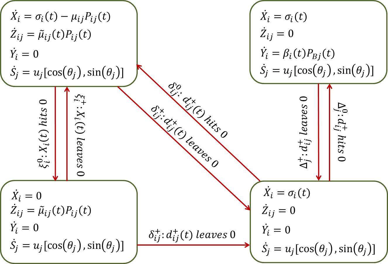
Figure 2: One target $i$ and one agent $j$ hybrid automaton

Observe that each of the events in Table I causes a change in at least one of the state variables in (5), (7), (8). For example, $\xi_{i}^{0}$ (i.e., the queue at target $i$ is emptied) causes a switch in (5) from $\dot{X}_{i}(t)=\sigma_{i}(t)-\mu_{ij}p_{ij}(t)$ to $\dot{X}_{i}(t)=0$. Also note that we have omitted an event $\zeta_{ij}^{+}$ for $Z_{ij}(t)$ becoming strictly positive since this event is immediately induced by $\delta_{ij}^{0}$ when agent $j$ comes within range of target $i$ and starts collecting data causing $Z_{ij}(t)>0$ if $Z_{ij}(t)=0$ and $X_{i}(t)>0$. Finally, note that all events are directly observable during the execution of any agent trajectory and they do not depend on our flow-based queueing model. For example, if $X_{i}(t)$ becomes zero, this defines event $\xi_{i}^{0}$ regardless of whether the corresponding queue is based on a flow or on discrete data packets; this observation is very useful in the sequel. A high-level hybrid automaton is presented in Fig. 2 for a single target $i$ and one agent $j$ system. This automaton becomes much more complicated once more targets and agents are included.

II-A Performance Measures

Our objective is to maintain minimal data content at all target queues while also maximizing the contents of the delivered data at the base queues. Thus, we define $J_{1}(t)$ to be the weighted sum of expected target queue content (recalling that $\{\sigma_{i}(t)\}$ are random processes):

$$J_{1}(t)=E\big{[}\sum\limits_{i=1}^{M}\alpha_{i}X_{i}(t)\big{]}$$ (10)

where the weight $\alpha_{i}$ represents the relative importance factor of target $i$. Similarly, we define a weighted sum of expected base queue content:

$$J_{2}(t)=E\big{[}\sum\limits_{i=1}^{M}\alpha_{i}Y_{i}(t)\big{]}$$ (11)

Therefore, a tentative optimization objective is the convex combination of (10) and (11) leading to the minimization problem:

$$\min\limits_{\mathbf{u(t),\boldsymbol{\theta}(t)}}J(T)=\frac{1}{T}\int_{0}^{T}\Big{(}qJ_{1}(t)-(1-q)J_{2}(t)\Big{)}dt$$ (12)

where $\mathbf{u}$ and $\boldsymbol{\theta}$ are the vectors formed by the agent speed and headings and $q\in[0,1]$ is a weight capturing the relative importance of collected data as opposed to delivered data.

This performance measure captures the collection and delivery of data which are processes taking place while an agent is connected to any of the targets or the base. However, it lacks any information regarding the interaction of an agent with the environment when this agent is not connected to any target or base and is due to the fact that the environment has only a finite number of points of interest (targets). This motivates two new performance measures we introduce next.

Agent Utilization: In accessing the targets, we must ensure that the agents maximize their utilization, i.e., the fraction of time spent performing a useful task by being within range of a target or the base. Equivalently, we aim to minimize the non-productive idling time of each agent during which it is not visiting any target or the base. Using (9), agent $j$ is idling when $d_{ij}^{+}(t)>0$ for all $i$ and $d_{\!{}_{Bj}}^{+}(t)>0$. We define the idling function $I_{j}(t)$ as follows:

$$I_{j}(t)=\log\Bigg{(}1+d_{\!{}_{Bj}}^{+}(t)\prod_{i=1}^{M}d_{ij}^{+}(t)\Bigg{)}$$ (13)

This function has the following properties. First, $I_{j}(t)=0$ if and only if the product term inside the bracket is zero, i.e., agent $j$ is visiting a target or the base; otherwise, $I_{j}(t)>0$. Second, $I_{j}(t)$ is monotonically nondecreasing in the number of targets $M$. The logarithmic function is selected to prevent the value of $I_{j}(t)$ from dominating those of $J_{1}(\cdot)$ and $J_{2}(\cdot)$ when included in a single objective function. Thus, we define:

$$J_{3}(t)=E\big{[}\sum\limits_{j=1}^{N}I_{j}(t)\big{]}$$ (14)

Note that $I_{j}(t)$ is also a random variable since it is a function of the agent states $s_{j}(t)$, $j=1,\dots,N$.

Event Excitation: As mentioned in the Introduction, our goal is to develop an event-driven approach for on-line trajectory optimization. In other words, we seek a controller whose actions are based on events observed during the operation of the hybrid system described earlier. Clearly, the premise of this approach is that the events involved are observable so as to “excite” the underlying event-driven controller. However, it is not always obvious that these events actually take place under every feasible control, in which case the controller may be useless. This is illustrated in Fig. 3 where two different trajectories are shown for the agent. The blue and red trajectories pass through none of the targets. Consequently, there is an infinite number of trajectories for which the value of the objective function in (12) is given by

$$J(T)=\frac{q}{T}\int_{0}^{T}t\sigma_{i}(t)dt\$$ (15)

which is simply the total amount of data generated at all targets through (5). This cannot be affected by any event-driven control action, since none of the events in Table I is excited. Clearly, the same is true for $J_{3}(t)$ in (14).

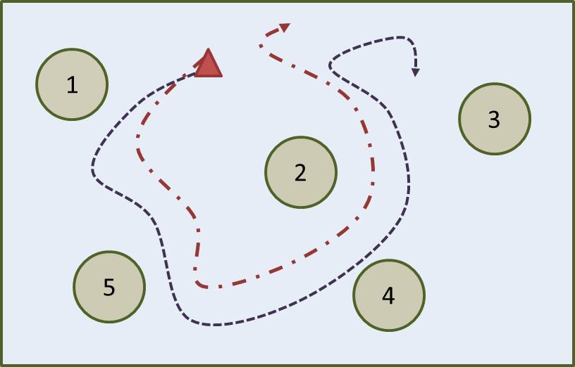
Figure 3: Two trajectories with same objective function value

To address this issue, our goal is to “spread” each target cost (accumulated data) $X_{i}(t)$ over all $w\in S$. This will create a potential field throughout the mission space. Following [25], we begin by determining the convex hull produced by the targets, since the trajectories need not go outside this polygon. Let $\mathcal{T}=\{w_{1},w_{2},\cdots,w_{M}\}$ be the set of all target points. Then, their convex hull is

$$\mathcal{C}=\bigg{\{}\sum_{i=1}^{M}\beta_{i}w_{i}|\sum_{i}\beta_{i}=1,\forall i,~{}\beta_{i}\geq 0\bigg{\}}$$ (16)

Given that $\mathcal{C}\subset S$, we seek a function $R(w,t)$ that satisfies the following property for some constants $c_{i}>0$:

$$\int_{\mathcal{C}}R(w,t)dw=\sum_{i=1}^{M}c_{i}X_{i}(t)$$ (17)

Thus, $R(w,t)$ can be viewed as a time-varying density function defined for all points $w\in\mathcal{C}$ which generates a total cost equivalent to a weighted sum of the target data $X_{i}(t)$, $i=1,\ldots,M$. Letting $d_{i}^{+}(w)=\max(\|w-w_{i}\|,r_{i})$, where $r_{i}=\min_{j}{r_{ij}}$, we then define:

$$R(w,t)=\sum_{i=1}^{M}\frac{\alpha_{i}X_{i}(t)}{d_{i}^{+}(w)}$$ (18)

Intuitively, a target’s cost (numerator above) is spread over all $w\in S$ so as to obtain the “total weighted cost density” at $w$. Note that $d_{i}^{+}(w)$ is defined to ensure that the target cost remains positive and fixed for all points $w\in C(w_{i})$. In order to illustrate this construction, Fig. 4(a) shows a sample mission space with 9 target locations and Fig 4(b) shows the value of $R(w,t)$ at a specific time $t$.

Proposition 1

There exist $c_{i}>0$, $i=1,\ldots,M$, such that:

$$\int_{\mathcal{C}}R(w,t)dw=\sum_{i=1}^{M}c_{i}x_{i}(t)$$ (19)

Proof:

See Appendix A. ∎

Using the same idea for the base, we define

$$R_{\!{}_{Bj}}(w,t)=\frac{\sum_{i=1}^{M}\alpha_{i}Z_{ij}}{d_{\!{}_{B}}^{+}(w)}$$ (20)

where $d_{\!{}_{B}}^{+}(w)=\max(\|w_{\!{}_{B}}-w\|,r_{\!{}_{B}})$ is a constant and $r_{\!{}_{B}}=\min_{j}{r_{\!{}_{Bj}}}$.

Proposition 19 asserts that the total cost due to data accumulated at targets may indeed be spread over all points in the mission space allowing an agent to “interact” with these points through the resulting potential field. In order to capture this interaction (see also [25]), we define the travel cost for an agent $j$ to reach point $w$ as the quadratic of the distance between them $\|s_{j}(t)-w\|^{2}$ and the total travel cost as

$$P(w,\mathbf{s}(t))=\sum_{j=1}^{N}\|s_{j}(t)-w\|^{2}$$ (21)

Using these definitions we can now introduce a new performance metric:

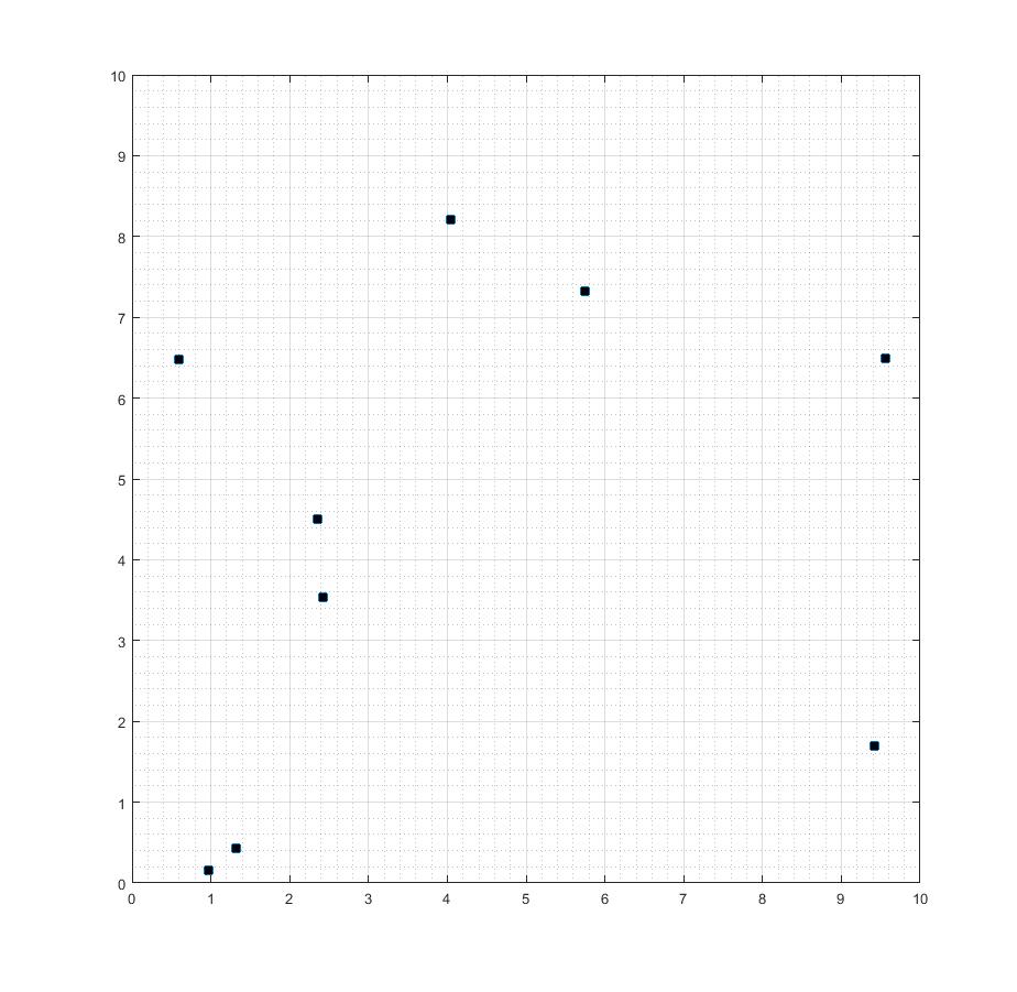
(a) Mission Space with dots as target locations

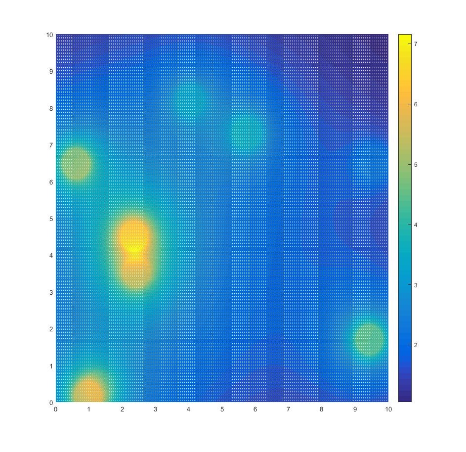
(b) $R$ Function at a sample time $t$

Figure 4: $R$ function illustration

Terminal Cost: Since we address the data harvesting problem over a finite interval $T$, we define a terminal cost at $T$ capturing the expected value of the amount of data left on board the agents:

$$J_{f}(T)=\frac{1}{T}E\big{[}\sum\limits_{i=1}^{M}\sum\limits_{j=1}^{N}\alpha_{i}Z_{ij}(T)\big{]}$$ (23)

Clearly, the effect of this term vanishes as $T\rightarrow\infty$ as long as all $E[Z_{ij}(T)]$ remains bounded. Moreover, if we constrain trajectories to be periodic, this terminal cost may be omitted. Finally, for simplicity, we will assume that $\alpha_{i}=1$ for all $i$.

II-B Optimization Problem

We can now formulate a stochastic optimization problem $\mathbf{P1}$ where the control variables are the agent speeds and headings denoted by the vectors $\mathbf{u}(t)=[u_{1}(t),\dots,u_{N}(t)]$ and $\boldsymbol{\theta}(t)=[\theta_{1}(t),\dots,\theta_{N}(t)]$ respectively (omitting their dependence on the full system state at $t$). Combining the components in (14), (22) and (23) we obtain:

$$\min\limits_{\mathbf{u(t),\boldsymbol{\theta}(t)}}J(T)= \frac{1}{T}\int_{0}^{T}\Big{(}\frac{q}{M_{X}}J_{1}(t)-\frac{(1-q)}{M_{Y}}J_{2}(t)$$ (24)

$$+\frac{1}{M_{I}}J_{3}(t)+\frac{1}{M_{R}}J_{4}(t)\Big{)}dt+\frac{1}{M_{Z}}J_{f}(T)$$

where we introduce the normalizing factors $M_{X}$, $M_{Y}$, $M_{I}$, $M_{R}$ and $M_{Z}$. This normalization ensures that all different components of $J(T)$ are in the same range so that none of them may dominate any other. We use an upper bound for the value of each component as follows, where we assume that $\sigma_{i}(0)>0$ w.p. 1:

$$M_{X} =M_{Y}=M_{Z}=T\sum_{i}\sigma_{i}(0)$$ (25)

$$M_{I} =\log\Big{(}1+\sqrt{L_{1}^{2}+L_{2}^{2}}^{M+1}\Big{)}$$ (26)

$$M_{R} =\frac{TL_{1}L_{2}(L_{1}^{2}+L_{2}^{2})}{r}\sum_{i}\sigma_{i}(0),r=\frac{\sum_{i}r_{i}}{M}$$ (27)

where $L_{1}$ and $L_{2}$ define the size of the rectangular mission space (the normalization factors can easily be adapted to different mission space shapes). Observe that an unattainable lower bound of the total objective function is $-(1-q)$ which occurs if $J_{1}=J_{3}=J_{4}=0$ and $J_{2}$ is at its maximum of 1. If $q=0$, then the lower bound is at its minimum of -1.

III Optimization Methodology

In this section, we consider problem $\mathbf{P1}$ in a setting where all data arrival processes are deterministic, so that all expectations in (10)-(23) degenerate to their arguments. We proceed with a standard Hamiltonian analysis leading to a Two Point Boundary Value Problem (TPBVP) [26] where the states and costates are known at $t=0$ and $t=T$ respectively. We define the costate vector associated to (1):

$$\boldsymbol{\lambda} (t)=[\lambda_{1}(t),\dots,\lambda_{M}(t),\gamma_{1}(t),\dots,\gamma_{M}(t),$$

$$\phi_{11}(t),\dots,\phi_{MN}(t),\eta_{1}^{x}(t),\eta_{1}^{y}(t),\dots,\eta_{N}^{x}(t),\eta_{N}^{y}(t)]$$ (28)

The Hamiltonian is

$$H(\mathbf{X},{\boldsymbol{\lambda}},\mathbf{u},{\boldsymbol{\theta}})=\frac{1}{T}\Big{[}qJ_{1}(t)-(1-q)J_{2}(t)+J_{3}(t)+J_{4}(t)\Big{]}$$

$$+\sum_{i}\lambda_{i}(t)\dot{X}_{i}(t)+\sum_{i}\gamma_{i}(t)\dot{Y}_{i}(t)+\sum_{i}\sum_{j}\phi_{ij}(t)\dot{Z}_{ij}(t)$$

$$+\sum_{j}\big{(}\eta_{j}^{x}(t)u_{j}(t)\cos\theta_{j}(t)+\eta_{j}^{y}(t)u_{j}(t)\sin\theta_{j}(t)\big{)}$$ (29)

where the costate equations are

$$\eta_{j}^{x}(T)=\eta_{j}^{y}(T)=0$$

From (29), after some trigonometric manipulations, we get

where $\tan\psi_{j}(t)=\frac{\eta_{j}^{x}(t)}{\eta_{j}^{y}(t)}$ for $\eta_{j}^{y}(t)\neq 0$ and $\psi_{j}(t)=\mbox{sgn}{\eta_{j}^{x}(t)}\frac{\pi}{2}$ if $\eta_{j}^{y}(t)=0$. Applying the Pontryagin principle to (29) with $(\mathbf{u}^{\ast},{\boldsymbol{\theta}}^{\ast})$ being the optimal control, we have:

$$H(\mathbf{X}^{\ast},{\boldsymbol{\lambda}}^{\ast},\mathbf{u}^{\ast},{\boldsymbol{\theta}}^{\ast})=\min\limits_{\mathbf{u}(t),\boldsymbol{\theta}(t)}H(\mathbf{X},{\boldsymbol{\lambda}},\mathbf{u},{\boldsymbol{\theta}})$$ (31)

From (30) we see that we can always set the control $\theta_{j}(t)$ to ensure that $\mbox{sgn}{\eta_{j}^{y}(t)}\sin(\theta_{j}(t)+\psi_{j}(t))<0$. Hence, recalling that $0\leq u_{j}(t)\leq 1$,

$$u_{j}^{\ast}(t)=1$$ (32)

and

$$\sin(\theta_{j}^{*}(t)+\psi_{j}(t))=1 \mbox{ if }\mu_{j}^{y}(t)<0$$

$$\sin(\theta_{j}^{*}(t)+\psi_{j}(t))=-1 \mbox{ if }\mu_{j}^{y}(t)>0$$ (33)

Following the Hamiltonian definition in (29) we have:

$$\frac{\partial H}{\partial\theta_{j}}=-\eta_{j}^{x}(t)u_{j}(t)\sin\theta_{j}(t)+\eta_{j}^{y}(t)u_{j}(t)\cos\theta_{j}(t)$$ (34)

and setting $\frac{\partial H}{\partial\theta_{j}}=0$ the optimal heading $\theta_{j}^{\ast}(t)$ should satisfy:

$$\tan\theta_{j}^{\ast}(t)=\frac{{\eta_{j}^{y}}(t)}{{\eta_{j}^{x}}(t)}$$ (35)

Since $u_{j}^{\ast}(t)=1$, we only need to evaluate $\theta_{j}^{\ast}(t)$ for all $t\in[0,T]$. This is accomplished by discretizing the problem in time and numerically solving a TPBVP with a forward integration of the state and a backward integration of the costate. Solving this problem becomes intractable as the number of agents and targets grows. The fact that we are dealing with a hybrid dynamic system further complicates the solution of a TPBVP. On the other hand, it enables us to make use of Infinitesimal Perturbation Analysis (IPA) [24] to carry out the parametric trajectory optimization process discussed in the next section. In particular, we propose a parameterization of agent trajectories allowing us to utilize IPA to obtain an unbiased estimate for the objective function gradient with respect to the trajectory parameters.

III-A Agent Trajectory Parameterization and Optimization

The key idea is to represent each agent’s trajectory through general parametric equations

$$\begin{array}[c]{ll}s_{j}^{x}(t)=f(\Theta_{j},\rho_{j}(t)),\text{ \ }\quad s_{j}^{y}(t)=g(\Theta_{j},\rho_{j}(t))&\end{array}$$ (36)

where the function $\rho_{j}(t)$ controls the position of the agent on its trajectory at time $t$ and $\Theta_{j}$ is a vector of parameters controlling the shape and location of the agent $j$ trajectory. Let $\Theta=[\Theta_{1},\dots,\Theta_{N}]$. We now replace problem $\mathbf{P1}$ in (II-B) by problem $\mathbf{P2}$:

$$\begin{split}\min\limits_{\Theta\in F_{\Theta}}&\frac{1}{T}\int_{0}^{T}\Big{[}qJ_{1}(\Theta,t)-(1-q)J_{2}(\Theta,t)+J_{3}(\Theta,t)\\ &+J_{4}(\Theta,t)\Big{]}dt+J_{f}(\Theta,T)\end{split}$$ (37)

where we return to allowing arbitrary stochastic data arrival processes $\{\sigma_{i}(t)\}$ so that $\mathbf{P2}$ is a parametric stochastic optimization problem with the feasible parameter set $F_{\Theta}$ appropriately defined depending on (36). The cost function in (37) is written as

$$J(\Theta,T;\mathbf{X}(\Theta,0))=E[\mathcal{L}(\Theta,T;\mathbf{X}(\Theta,0))]$$

where $\mathcal{L}(\Theta,T;\mathbf{X}(\Theta,0))$ is a sample function defined over $[0,T]$ and $\mathbf{X}(\Theta,0)$ is the initial value of the state vector. For convenience, in the sequel we will use $\mathcal{L}_{i}$, $i=1,\ldots,4$, and $\mathcal{L}_{f}$ to denote sample functions of $J_{i}$, $i=1,\ldots,4$, and $J_{f}$ respectively. Note that in (37) we suppress the dependence of the four objective function components on the controls $\mathbf{u}(t)$ and $\boldsymbol{\theta}(t)$ and stress instead their dependence on the parameter vector $\Theta$.

In the rest of the paper, we will consider two families of trajectories motivated by a similar approach used in the multi-agent persistent monitoring problem in [23]: elliptical trajectories and a more general Fourier series trajectory representation better suited for non-uniform target topologies. The hybrid dynamics of the data harvesting system allow us to apply the theory of IPA [24] to obtain on line the gradient of the sample function $\mathcal{L}(\Theta,T;\mathbf{X}(\Theta,0))$ with respect to $\Theta$. The value of the IPA approach is twofold: $(i)$ The sample gradient $\nabla\mathcal{L}(\Theta,T)$ can be obtained on line based on observable sample path data only, and $(ii)$ $\nabla\mathcal{L}(\Theta,T)$ is an unbiased estimate of $\nabla J(\Theta,T)$ under mild technical conditions as shown in [24]. Therefore, we can use $\nabla\mathcal{L}(\Theta,T)$ in a standard gradient-based stochastic optimization algorithm

$$\Theta^{l+1}=\Theta^{l}-\boldsymbol{\nu}_{l}\nabla\mathcal{L}(\Theta^{l},T),\text{ \ }l=0,1,\ldots$$ (38)

to converge (at least locally) to an optimal parameter vector $\Theta^{\ast}$ with a proper selection of a step-size sequence $\{\boldsymbol{\nu}_{l}\}$ [27]. We emphasize that this process is carried out on line, i.e., the gradient is evaluated by observing a trajectory with given $\Theta$ over $[0,T]$ and is iteratively adjusted until convergence is attained.

III-A1 IPA Calculus Review and Implementation

Based on the events defined earlier, we will specify event time derivative and state derivative dynamics for each mode of the hybrid system. In this process, we will use the IPA notation from [24] so that ${\tau_{k}}$ is the $k$th event time in an observed sample path of the hybrid system and ${\tau_{k}^{\prime}}=\frac{d\tau_{k}}{d\Theta}$, $\mathcal{X}^{\prime}(t)=\frac{d\mathcal{X}}{d\Theta}$ are the Jacobian matrices of partial derivatives with respect to all components of the controllable parameter vector $\Theta$. Throughout the analysis we will be using $(\cdot)^{\prime}$ to show such derivatives. We will also use $f_{k}(t)=\frac{d\mathcal{X}}{dt}$ to denote the state dynamics in effect over an interevent time interval $[{\tau_{k},\tau_{k+1})}$. We review next the three fundamental IPA equations from [24] based on which we will proceed.

First, events may be classified as exogenous or endogenous. An event is exogenous if its occurrence time is independent of the parameter $\Theta$, hence ${\tau_{k}^{\prime}}=0$. Otherwise, an endogenous event takes place when a condition $g_{k}(\Theta,\mathcal{X})=0$ is satisfied, i.e., the state $\mathcal{X}(t)$ reaches a switching surface described by $g_{k}(\Theta,\mathcal{X})$. In this case, it is shown in [24] that

$${\tau_{k}^{\prime}}=-\Big{(}\frac{dg_{k}}{d\mathcal{X}}f_{k}(\tau_{k}^{-})\Big{)}^{-1}\Big{(}g^{\prime}_{k}+\frac{dg_{k}}{d\mathcal{X}}{\mathcal{X}^{\prime}(\tau_{k}^{-})}\Big{)}$$ (39)

as long as $\frac{\partial g_{k}}{\partial\mathcal{X}}f_{k}(\tau_{k}^{-})\neq 0$. It is also shown in [24] that the state derivative $\mathcal{X}^{\prime}(t)$ satisfies

$$\frac{d}{dt}\mathcal{X}^{\prime}(t)=\frac{df_{k}}{d\mathcal{X}}\mathcal{X}^{\prime}(t)+f^{\prime}_{k}(t),\text{ \ \ }t\in[{\tau_{k},\tau_{k+1})}$$ (40)

$$\mathcal{X}^{\prime}(\tau_{k}^{+})=\mathcal{X}^{\prime}(\tau_{k}^{-})+[f_{k-1}(\tau_{k}^{-})-f_{k}(\tau_{k}^{+})]{\tau_{k}}^{\prime}$$ (41)

Then, $\mathcal{X}^{\prime}(t)$ for $t\in[{\tau_{k},\tau_{k+1})}$ is calculated through

$$\mathcal{X}^{\prime}(t)=\mathcal{X}^{\prime}(\tau_{k}^{+})+\int_{\tau_{k}}^{t}\frac{d}{dt}\mathcal{X}^{\prime}(t)dt$$ (42)

Table I contains all possible endogenous event types for our hybrid system. To these, we add exogenous events $\kappa_{i}$, $i=1,...,M$, to allow for possible discontinuities (jumps) in the random processes $\{\sigma_{i}(t)\}$ which affect the sign of $\sigma_{i}(t)-\mu_{ij}p_{ij}(t)$ in (5). We will use the notation $e(\tau_{k})$ to denote the event type occurring at $t=\tau_{k}$ with $e(\tau_{k})\in E$, the event set consisting of all endogenous and exogenous events. Finally, we make the following assumption which is needed in guaranteeing the unbiasedness of the IPA gradient estimates: $(\mathbf{A6})$ Two events occur at the same time w.p. $0$ unless one is directly caused by the other.

III-A2 Objective Function Gradient

The sample function gradient $\nabla\mathcal{L}(\Theta,T)$ needed in (38) is obtained from (37) assuming a total number of $K$ events over $[0~{}T]$ with $\tau_{\!{}_{K+1}}=T$ and $\tau_{0}=0$:

The last step follows from the continuity of the state variables which causes adjacent limit terms in the sum to cancel out. Therefore, $\nabla\mathcal{L}(\Theta,T)$ does not have any direct dependence on any $\tau_{k}^{\prime}$; this dependence is indirect through the state derivatives involved in the four individual gradient terms.

Referring to (10), the first term in (43) involves $\nabla\mathcal{L}_{1}(\Theta,t)$ which is as a sum of $X_{i}^{\prime}(t)$ derivatives. Similarly, $\nabla\mathcal{L}_{2}(\Theta,t)$ is a sum of $Y_{i}^{\prime}(t)$ derivatives and $\nabla\mathcal{L}_{f}(\Theta,T)$ requires only $Z_{ij}^{\prime}(T)$. The third term, $\nabla\mathcal{L}_{3}(\Theta,t)$, requires derivatives of $I_{j}(t)$ in (13) which depend on the derivatives of the max function in (9) and the agent state derivatives $s_{j}^{\prime}(t)$ with respect to $\Theta$. The term $\nabla\mathcal{L}_{4}(\Theta,t)$ needs the values of $X_{i}^{\prime}(t)$ and $Z_{ij}^{\prime}(t)$. The gradients of the last two terms are derived in the appendix. Possible discontinuities in these derivatives occur when any of the last four events in Table I takes place.

In summary, the evaluation of (43) requires the state derivatives $X_{i}^{\prime}(t)$, $Z_{ij}^{\prime}(t)$, $Y_{i}^{\prime}(t)$, and $s_{j}^{{\prime}}(t)$. The latter are easily obtained for any specific choice of $f$ and $g$ in (36) and are shown in Appendix B. The former require a rather laborious use of (39)-(41) which, however, reduces to a simple set of state derivative dynamics as shown next.

Proposition 2

: After an event occurrence at $t=\tau_{k}$, the state derivatives $X_{i}^{\prime}(\tau_{k}^{+})$, $Y_{i}^{\prime}(\tau_{k}^{+})$, $Z_{ij}^{\prime}(\tau_{k}^{+})$, with respect to the controllable parameter $\Theta$ satisfy the following:

$$X_{i}^{\prime}(\tau_{k}^{+})=\left\{\begin{array}[c]{ll}0&\text{if }e(\tau_{k})=\xi_{i}^{0}\\ X_{i}^{\prime}(\tau_{k}^{-})-\mu_{il}p_{il}(\tau_{k}){\tau_{k}^{\prime}}&\text{if }e(\tau_{k})=\delta_{ij}^{+}\\ X_{i}^{\prime}(\tau_{k}^{-})&\text{otherwise}\end{array}\right.$$

where $l\neq j$ with $p_{il}(\tau_{k})>0$ if such $l$ exists and ${\tau_{k}^{\prime}=}\frac{\partial d_{ij}(s_{j})}{\partial s_{j}}s_{j}^{\prime}\left(\frac{\partial d_{ij}(s_{j})}{\partial s_{j}}\dot{s}_{j}(\tau_{k})\right)^{-1}$.

$$Y_{i}^{\prime}(\tau_{k}^{+}) =\left\{\begin{array}[c]{ll}Y_{i}^{\prime}(\tau_{k}^{-})+Z_{ij}^{\prime}(\tau_{k}^{-})&\text{if }e(\tau_{k})=\zeta_{ij}^{0}\\ Y_{i}^{\prime}(\tau_{k}^{-})&\text{otherwise}\end{array}\right.$$

$$Z_{ij}^{\prime}(\tau_{k}^{+}) =\left\{\begin{array}[c]{ll}0&\text{if }e(\tau_{k})=\zeta_{ij}^{0}\\ Z_{ij}^{\prime}(\tau_{k}^{-})+X_{i}^{\prime}(\tau_{k}^{-})&\text{if }e(\tau_{k})=\xi_{i}^{0}\\ Z_{ij}^{\prime}(\tau_{k}^{-})&\text{otherwise}\end{array}\right.$$

where $e(\tau_{k})=\xi_{i}^{0}$ occurs when $j$ is connected to target $i$.

Proof:

: See (76), (87), (95), (93), (79), (88), (90), (82) in Appendix D. ∎

This result shows that only three of the events in $E$ can actually cause discontinuous changes to the state derivatives. Further, note that $X_{i}^{\prime}(t)$ is reset to zero after a $\xi_{i}^{0}$ event. Moreover, when such an event occurs, note that $Z_{ij}^{\prime}(t)$ is coupled to $X_{i}^{\prime}(t)$. Similarly for $Z^{\prime}_{ij}(t)$ and $Y^{\prime}_{i}(t)$ when event $\zeta_{ij}^{0}$ occurs, showing that perturbations in $\Theta$ can only propagate to an adjacent queue when that queue is emptied.

Proposition 3

: The state derivatives $X_{i}^{\prime}(\tau_{k+1}^{-})$, $Y_{i}^{\prime}(\tau_{k+1}^{-})$ with respect to the controllable parameter $\Theta$ satisfy the following after an event occurrence at $t=\tau_{k}$:

$$X_{i}^{\prime}(\tau_{k+1}^{-}) =\left\{\begin{array}[c]{ll}0&\text{if }e(\tau_{k})=\xi_{i}^{0}\\ X_{i}^{\prime}(\tau_{k}^{+})-\int_{\tau_{k}}^{\tau_{k+1}}\mu_{ij}p_{ij}^{\prime}(u)du&\text{otherwise}\end{array}\right.$$

$$Y_{i}^{\prime}(\tau_{k+1}^{-}) =Y_{i}^{\prime}(\tau_{k}^{+})+\int_{\tau_{k}}^{\tau_{k+1}}\beta_{i}^{\prime}(u)du$$

where $j$ is such that $p_{ij}(t)>0$, $t\in[{\tau_{k},\tau_{k+1})}$.

Proof:

: See (75), (78) and (80) in Appendix D. ∎

Proposition 4

: The state derivatives $Z_{ij}^{\prime}(\tau_{k+1}^{+})$ with respect to the controllable parameter $\Theta$ satisfy the following after an event occurrence at $t=\tau_{k}$:
i- If $j$ is connected to target $i$,

$$Z_{ij}^{\prime}(\tau_{k+1}^{-})=\left\{\begin{array}[c]{ll}Z_{ij}^{\prime}(\tau_{k}^{+})\qquad\qquad\text{if }e(\tau_{k})=\xi_{i}^{0},\text{ }\zeta_{ij}^{0}\text{ or }\delta_{ij}^{+}&\\ Z_{ij}^{\prime}(\tau_{k}^{+})+\int_{\tau_{k}}^{\tau_{k+1}}\mu_{ij}p_{ij}^{\prime}(u)du\quad\text{otherwise}&\end{array}\right.$$

ii- If $j$ is connected to $B$ with $Z_{ij}(\tau_{k})>0$,

$$Z_{ij}^{\prime}(\tau_{k+1}^{-})=Z_{ij}^{\prime}(\tau_{k}^{+})-\int_{\tau_{k}}^{\tau_{k+1}}\beta_{ij}p_{Bj}^{\prime}(u)du$$

iii- Otherwise, $Z_{ij}^{\prime}(\tau_{k+1}^{-})=Z_{ij}^{\prime}(\tau_{k}^{+})$.

Proof:

: See (83), (84), (91) and (98) in Appendix D. ∎

Corollary 5

The state derivatives $X_{i}^{\prime}(t)$, $Z_{ij}^{\prime}(t)$, $Y_{i}^{\prime}(t)$ with respect to the controllable parameter $\Theta$ are independent of the random data arrival processes $\{\sigma_{i}(t)\}$, $i=1,\ldots,M$.

Proof:

: Follows directly from the three Propositions. ∎

There are a few important consequences of these results. First, as the Corollary asserts, one can apply IPA regardless of the characteristics of the random processes $\{\sigma_{i}(t)\}$. This robustness property does not mean that these processes do not affect the values of the $X_{i}^{\prime}(t)$, $Z_{ij}^{\prime}(t)$, $Y_{i}^{\prime}(t)$; this happens through the values of the event times ${\tau_{k}}$, $k=1,2,\ldots$, which are observable and enter the computation of these derivatives as seen above.

Second, the IPA estimation process is event-driven: $X_{i}^{\prime}(\tau_{k}^{+})$, $Y_{i}^{\prime}(\tau_{k}^{+})$, $Z_{ij}^{\prime}(\tau_{k}^{+})$ are evaluated at event times and then used as initial conditions for the evaluations of $X_{i}^{\prime}(\tau_{k+1}^{-})$, $Y_{i}^{\prime}(\tau_{k+1}^{-})$, $Z_{ij}^{\prime}(\tau_{k+1}^{-})$ along with the integrals appearing in Propositions 2,3 which can also be evaluated at $t=\tau_{k+1}$. Consequently, this approach is scalable in the number of events in the system as the number of agents and targets increases.

Third, despite the elaborate derivations in the Appendix, the actual implementation reflected by the three Propositions is simple. Finally, returning to (43), note that the integrals involving $\nabla\mathcal{L}_{1}(\Theta,t)$, $\nabla\mathcal{L}_{2}(\Theta,t)$ are directly obtained from $X_{i}^{\prime}(t)$, $Y_{i}^{\prime}(t)$, the integral involving $\nabla\mathcal{L}_{3}(\Theta,t)$ is obtained from straightforward differentiation of (13), and the final term is obtained from $Z_{ij}^{\prime}(T)$.

III-A3 Objective Function Optimization

This is carried out using (38) with an appropriate diminishing step size sequence.

Elliptical Trajectories: Elliptical trajectories are described by their center coordinates, minor and major axes and orientation. Agent $j$’s position $s_{j}(t)=[s_{j}^{x}(t),s_{j}^{y}(t)]$ follows the general parametric equation of the ellipse:

Here, $\Theta_{j}=[A_{j},B_{j},a_{j},b_{j},\phi_{j}]$ where $A_{j},B_{j}$ are the coordinates of the center, $a_{j}$ and $b_{j}$ are the major and minor axis respectively while $\phi_{j}\in[0,\pi)$ is the ellipse orientation which is defined as the angle between the $x$ axis and the major axis of the ellipse. The time dependent parameter $\rho_{j}(t)$ is the eccentric anomaly of the ellipse. Since the agent is moving with constant speed of 1 on this trajectory from (32), we have $\dot{s}_{j}^{x}(t)^{2}+\dot{s}_{j}^{y}(t)^{2}=1$ which gives

In the data harvesting problem, trajectories that do not pass through the base are inadmissible since there is no delivery of data. Therefore, we add a constraint to force the ellipse to pass through $w_{\!{}_{B}}=[w_{\!{}_{B}}^{x},w_{\!{}_{B}}^{y}]$ where:

$$\begin{split}w_{\!{}_{B}}^{x}=&A_{j}+a_{j}\cos\rho_{j}(t)\cos\phi_{j}-b_{j}\sin\rho_{j}(t)\sin\phi_{j}\\ w_{\!{}_{B}}^{y}=&B_{j}+a_{j}\cos\rho_{j}(t)\sin\phi_{j}+b_{j}\sin\rho_{j}(t)\cos\phi_{j}\end{split}$$ (45)

Using the fact that $\sin^{2}\rho(t)+\cos^{2}\rho(t)=1$ we define a quadratic constraint term added to $J(\Theta,T;\mathbf{X}(\Theta,0))$ with a sufficiently large multiplier. This can ensure the optimal path passes through the base location $w_{\!{}_{B}}$. We define $\mathcal{C}_{j}(\Theta_{j})$:

$$\mathcal{C}_{j}(\Theta_{j})=\big{(}1-f_{j}^{1}\cos^{2}\phi_{j}-f_{j}^{2}\sin^{2}\phi_{j}-f_{j}^{3}\sin 2\phi_{j}\big{)}^{2}$$ (46)

where $f_{j}^{1}=\big{(}\frac{w_{\!{}_{B}}^{x}-A_{j}}{a_{j}}\big{)}^{2}+\big{(}\frac{w_{\!{}_{B}}^{y}-B_{j}}{b_{j}}\big{)}^{2}$, $f_{j}^{2}=\big{(}\frac{w_{\!{}_{B}}^{x}-A_{j}}{b_{j}}\big{)}^{2}+\big{(}\frac{w_{\!{}_{B}}^{y}-B_{j}}{a_{j}}\big{)}^{2}$, $f_{j}^{3}=\frac{(b_{j}^{2}-a_{j}^{2})(w_{\!{}_{B}}^{x}-A_{j})(w_{\!{}_{B}}^{y}-B_{j})}{a_{j}^{2}b_{j}^{2}}$.

(a) TPBVP Trajectories for Case I

(b) Elliptical Trajectories for case I

(c) Fourier Trajectories for case I

Figure 5: Simulation results for the two-target and two-agent case

Multiple visits to the base may be needed during the mission time $[0,T]$. We can capture this by allowing an agent trajectory to consist of a sequence of admissible ellipses. For each agent, we define $\mathcal{E}_{j}$ as the number of ellipses in its trajectory. The parameter vector $\Theta_{j}^{\kappa}$ with $\kappa=1,\dots,\mathcal{E}_{j}$, defines the $\kappa th$ ellipse in agent $j$’s trajectory and $\mathcal{T}_{j}^{\kappa}$ is the time that agent $j$ completes ellipse $\kappa$. Therefore, the location of each agent is described through $\kappa$ during $[\mathcal{T}_{j}^{\kappa-1},\mathcal{T}_{j}^{\kappa}]$ where $\mathcal{T}_{j}^{0}=0$. Since we cannot optimize over all possible $\mathcal{E}_{j}$ for all agents, an iterative process needs to be performed in order to find the optimal number of segments in each agent’s trajectory. At each step, we fix $\mathcal{E}_{j}$ and find the optimal trajectory with that many segments. The process is stopped once the optimal trajectory with $\mathcal{E}_{j}$ segments is no better than the optimal one with $\mathcal{E}_{j}-1$ segments (obviously, this is generally not a globally optimal solution). We can now formulate the parametric optimization problem $\mathbf{P2_{e}}$ where $\Theta_{j}=[\Theta_{j}^{1},\dots,\Theta_{j}^{\mathcal{E}_{j}}]$ and $\Theta=[\Theta_{1},\dots,\Theta_{N}]$:

where $M_{C}$ is a large multiplier. The evaluation of $\nabla\mathcal{C}_{j}$ is straightforward and does not depend on any event (details are shown in Appendix B).

Fourier Series Trajectories: The elliptical trajectories are limited in shape and may not be able to cover many targets in a mission space. Thus, we next parameterize the trajectories using a Fourier series representation of closed curves [28]. Using a Fourier series function for $f$ and $g$ in (36), agent $j$’s trajectory can be described as follows with base frequencies $f_{j}^{x}$ and $f_{j}^{y}$:

The parameter $\rho(t)\in[0,2\pi]$, similar to elliptical trajectories, represents the position of the agent along the trajectory. In this case, forcing a Fourier series curve to pass through the base is easier. For simplicity, we assume a trajectory to start at the base and set $s_{j}^{x}(0)=w_{\!{}_{B}}^{x}$, $s_{j}^{y}(0)=w_{\!{}_{B}}^{y}$. Assuming $\rho(0)=0$, with no loss of generality, we can calculate the zero frequency terms by means of the remaining parameters:

$$a_{0,j}=w_{\!{}_{B}}^{x}-\displaystyle\sum_{n=1}^{\Gamma_{j}^{x}}a_{n,j}\sin(\phi_{n,j}^{x}),b_{0,j}=w_{\!{}_{B}}^{y}-\displaystyle\sum_{n=1}^{\Gamma_{j}^{y}}b_{n,j}\sin(\phi_{n,j}^{y})$$

The parameter vector for agent $j$ is $\Theta_{j}=[f_{j}^{x},a_{0,j},\ldots,a_{\Gamma_{j}^{x}},b_{0,j},\ldots,b_{\Gamma_{j}^{y}},\phi_{1,j},\ldots,\phi_{\Gamma_{j}^{x}},\xi_{1,j},\ldots,\xi_{\Gamma_{j}^{y}}]$ and $\Theta=[\Theta_{1},\ldots,\Theta_{N}]$. Note that the shape of the curve is fully captured by the ratio $f_{j}^{x}/f_{j}^{y}$, so that one of these two parameters can be kept constant. For the Fourier trajectories, the fact that $\mathbf{u}_{j}^{\ast}=1$ allows us to calculate $\dot{\rho}_{j}(t)$ as follows:

Problem $\mathbf{P2_{f}}$ is the same as $\mathbf{P2}$ but there are no additional constraints in this case:

IV Numerical Results

In this section numerical results are presented to illustrate our approach. The mission space $S$ is considered to be $[0,10]\times[0,10]$ in all cases. The first case we consider is a small mission to obtain the TPBVP results and confirm the fact that it is not scalable to bigger problems.

In Case I we consider a two-target, two-agent setting. We assume deterministic arrival processes with $\sigma_{i}=0.5$ for all $i$. For (3) and (4) we have used $p(w,v)=\max(0,1-\frac{d(w,v)}{r})$ where $r$ is the corresponding value of $r_{ij}$ or $r_{\!{}_{Bj}}$. We set $\mu_{ij}=100$ and $\beta_{ij}=500$ for all $i$ and $j$. Other parameters used are $q=0.5$, $r_{ij}=r_{\!{}_{Bj}}=0.5$ and $T=20$. The trajectory comparison from TPBVP, Elliptical and Fourier parametric solutions is shown in Figs. 5(a), 5(b), 5(c). In each figure, the trajectories are shown in the top part, while the actual objective function convergence behavior is hown in the middle graph. The lower graph shows the total amount of data at targets at any time (in blue) and the total amount of data at the base (in green).

In the TPBVP results, the main limitation is the number of the time steps in the discretization of the interval $[0,T]$, since the number of control values grows with it. To bring this into prospective, for this sample problem with $T=20$ we considered $300$ time steps, i.e., $300$ values for the heading of each agent need to be calculated, which brings the total number of controls to $600$. In contrast, for the same problem the total number of controls for the elliptical trajectories are $10$ parameters and for the Fourier trajectories it is $28$. This explains why the TPBVP cannot be a viable solution for larger values of $T$. Note that, in this scenario the total time is only 20 time steps so we can obtain a TPBVP solution. This, however, causes a poor representation for the parameterized trajectories which are spending significant time outside the convex hull since they have not converged after only 20 time steps.

In Table II, the actual values for $J^{\ast}$, $J_{1}^{\ast}$, $J_{2}^{\ast}$ are shown for the three different trajectories of Fig. 5(a).,5(b),5(c). Note that the objective is to minimize $J$ by minimizing $J_{1}-J_{2}$.

(a) Elliptical Trajectories for Case II

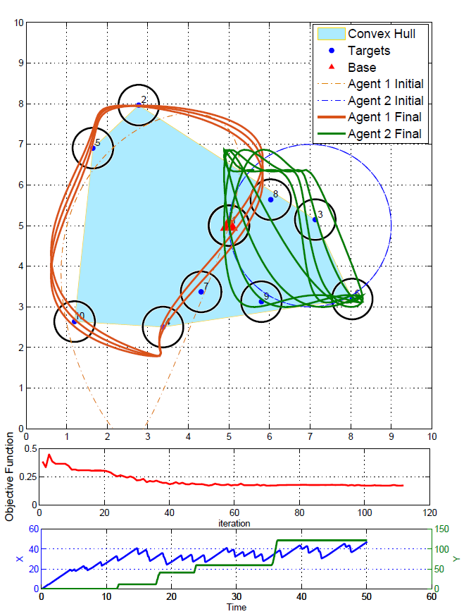
(b) Fourier Trajectories for Case II

Figure 6: Simulation results for 9-target and two-agent case

Next, in Case II we consider 9 targets and 2 agents. The base is located at the center of the mission space. We have $\sigma_{i}(t)=0.5$, $\mu_{ij}=50$ and $\beta_{ij}=500$ for all $i$ and $j$. Other parameters used are $q=0.5$, $r_{ij}=0.55,~{}r_{\!{}_{Bj}}=0.65$ and $T=50$. In Fig. 6(a) the solution with two ellipses in each agent’s trajectory is shown. As can be seen the trajectory correctly finds all the target locations and empties the target queues periodically. Fig. 6(b) shows the Fourier trajectories. The two graphs on the bottom show the objective function value and instantaneous total content at targets and base. The results for Case II are summarized in Table III.

TABLE II: Result Comparison for Case I

Method	$J^{*}$	$J_{1}^{*}$	$-J_{2}^{*}$
TPBVP	0.272	0.098	-0.038
Elliptical	0.255	0.092	-0.095
Fourier	0.202	0.089	-0.095

TABLE III: Results Comparison for Case II

Method	$J^{*}$	$J_{1}^{*}$	$-J_{2}^{*}$
Elliptical	0.19	0.090	-0.124
Fourier	0.18	0.069	-0.117

TABLE IV: Results Comparison for Case III

Method	$J^{*}$	$J_{1}^{*}$	$-J_{2}^{*}$
Elliptical	0.35	0.12	-0.09
Fourier	0.23	0.09	-0.1
Fourier (Stochastic Arrival)	0.23	0.13	-0.13

Case III has 12 targets that are uniformly distributed in the mission space. Here, we try to examine the robustness of our approach with respect to the arrival rate process at targets. We use the same parameters as in case II and solve the problem for deterministic $\sigma_{i}(t)=0.5$ using the elliptical trajectories and Fourier trajectories. The same mission is simulated assuming that ${\sigma_{i}(t)}$ is a stochastic process with piecewise linear arrival rate. The average arrival rate is kept at $0.5$. The results in Figs. 7(a),7(b),7(c) and Table IV show that the Fourier parametric trajectories achieve almost the same performance by the optimization algorithm in the stochastic setting.

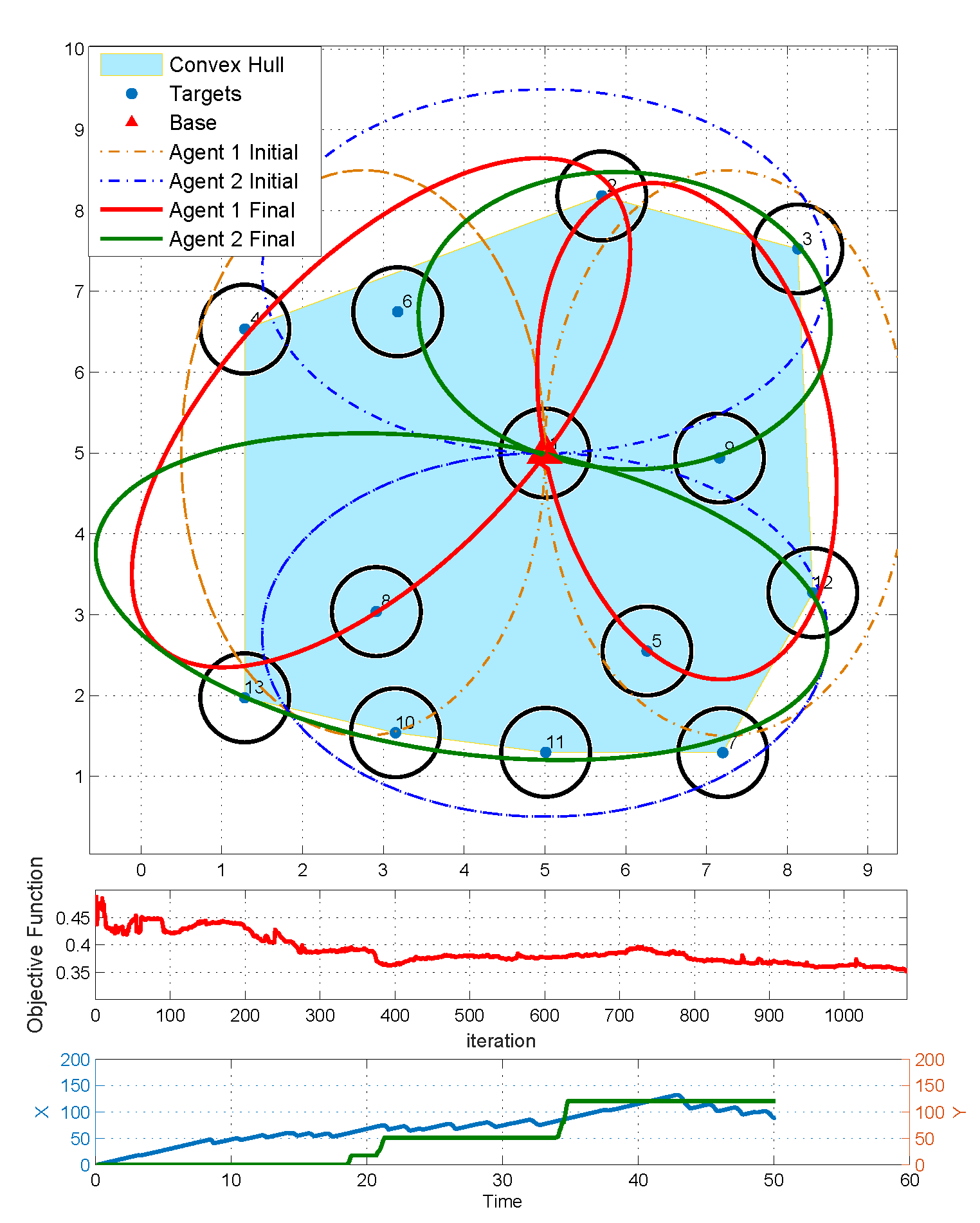
(a) Elliptical Trajectories for case III

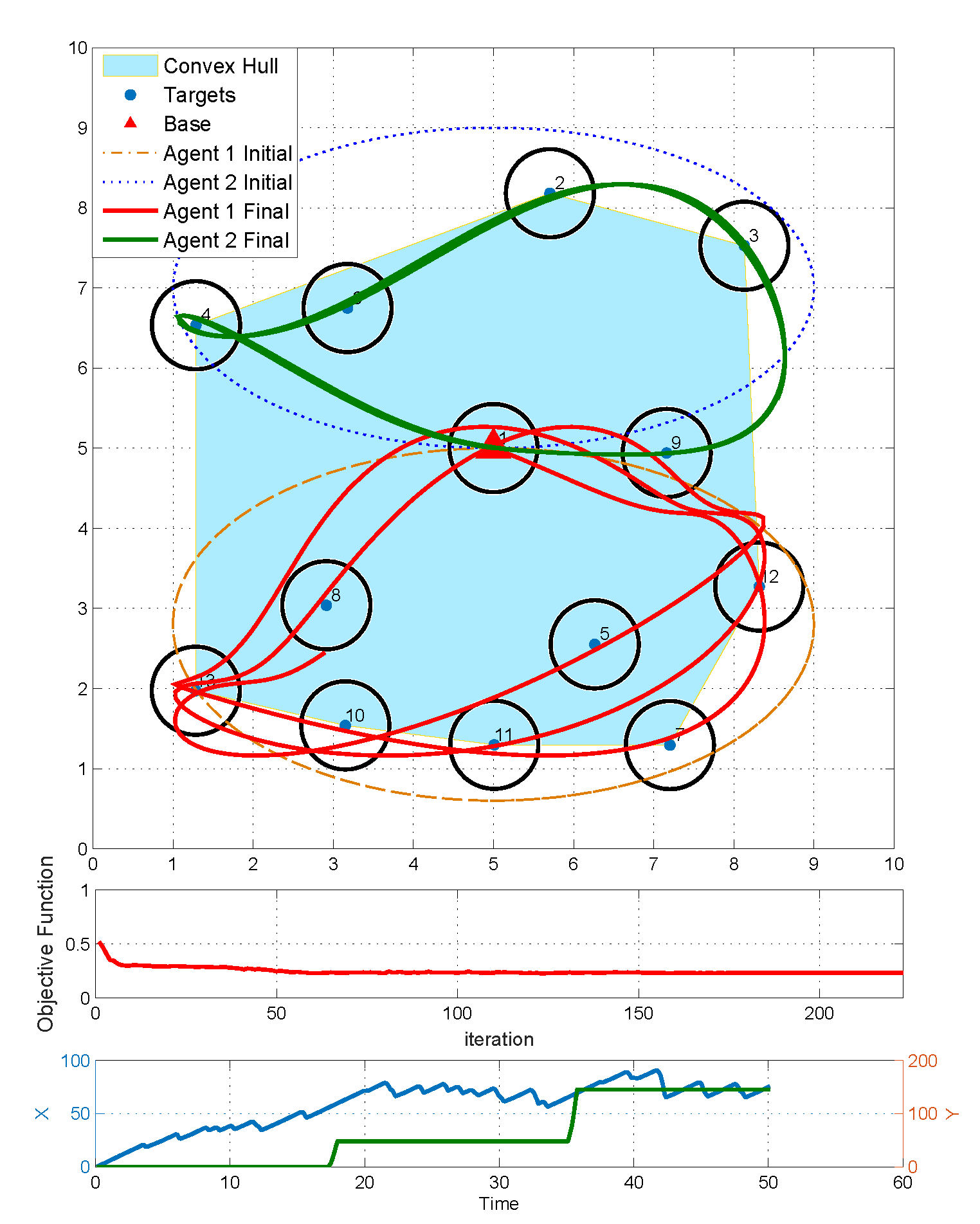
(b) Fourier Trajectories for case III

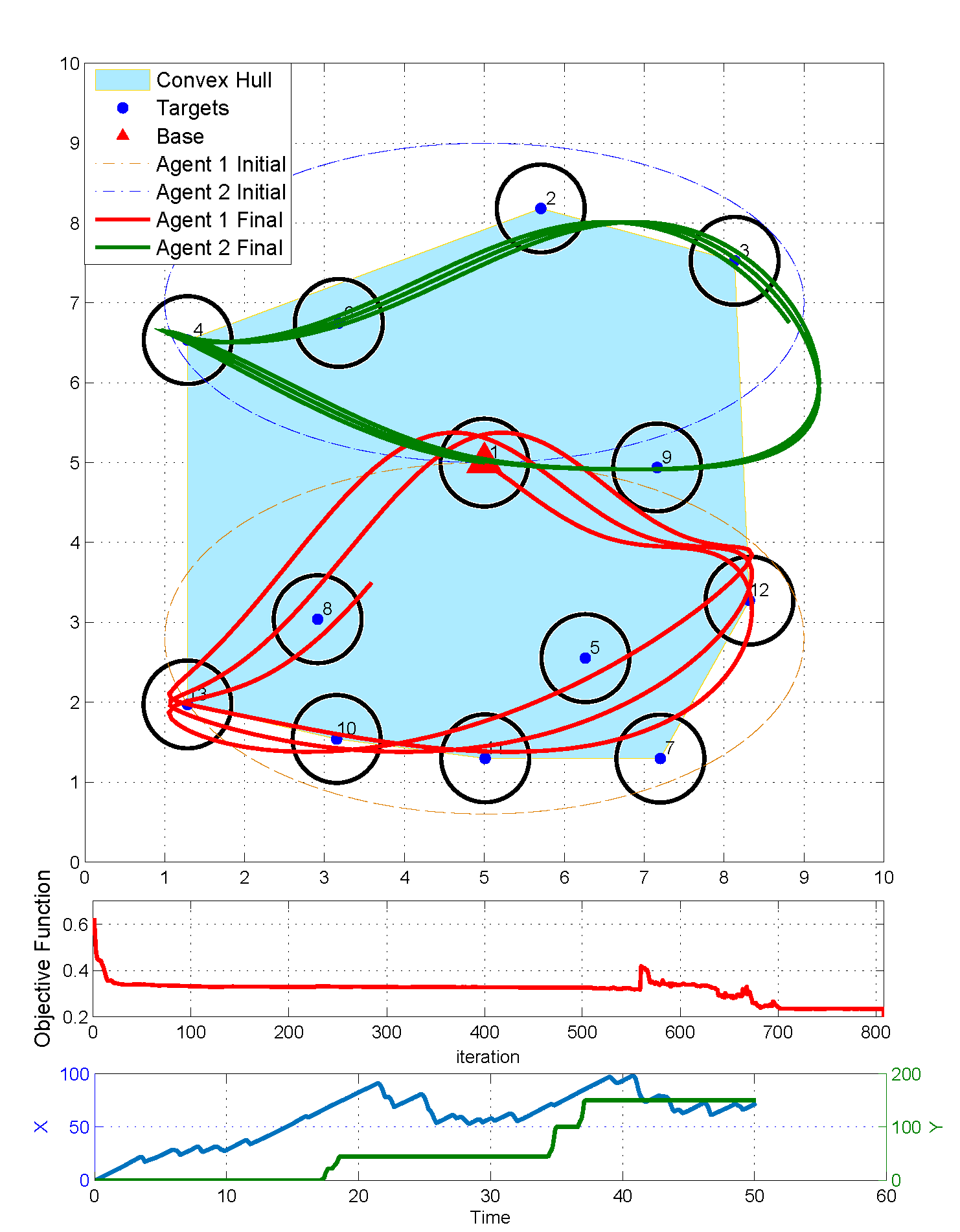
(c) Fourier Trajectories for case III with Stochastic Arrival

Figure 7: Simulation results for the 12-target and two-agent case

V Comparison with a Graph Based Algorithm

We begin with the observation that the final parametric trajectories provide a sequence of targets visits, similar to the functionality of a tour selection algorithm that uses the underlying graph topology of the mission space to determine such sequences.

We have compared the results of our approach with a graph topology algorithm called Path Splitter Heuristic (PSH) developed in [12]. This algorithm starts with the best Hamiltonian sequence and then uses a heuristic method to divide the Hamiltonian tour into several sub-tours that go through a few targets and then return to the base. The algorithm then provides a sequence of these sub-tours for each agent. We compare the sequences from Case I and Case II in both elliptical and Fourier trajectories and results are shown in Tables V and VI. For a fair comparison, we adopt each sequence and apply it with the system dynamics in our model, i.e., an agent can collect the data once within range of a target and the data collection does not happen instantaneously. This, however, is not the basic modeling assumption used in PSH, where agents pick up all the data at the target instantaneously once at the target location. We compare the sum total of data at targets and the base for $T=200$. A larger value of $T$ is used for this comparison in order to approximate infinite time results. These sequences are shown in Figs. 8(a), 8(b) and 8(c) where each color represents one agent trajectory. We can see from these comparisons that in the graph-based approach targets are completely divided between agents. This generates a spatial partitioning, giving each agent full responsibility for a set of targets. However, in the trajectory planning results, in most cases, we see a temporal partitioning where agents can visit the same targets but at different times of the mission. This clearly allows for more robustness with respect to potential agent failures or changes in an agent’s operation. Moreover, even though the computational complexity of the PSH algorithm and the parametric trajectory optimization approach are comparable, methods such as PSH need to re-solve the complete problem each time a new target may appear in the mission space. In contrast, the on-line event-driven parametric optimization process is a methodology designed to adapt to targets which may randomly appear in the mission space. These results are not necessarily aiming to prove performance enhancement but to put the two approaches into contrast in terms of suitability for online and offline applications. Also, PSH agent trajectories consist of straight line segments. These are not physically realizable, given limitations on the motion of agents which must smoothly turn direction from one target to the next. Whereas the parametrical trajectories are easier to realize by most of the agents given these motion limitations.

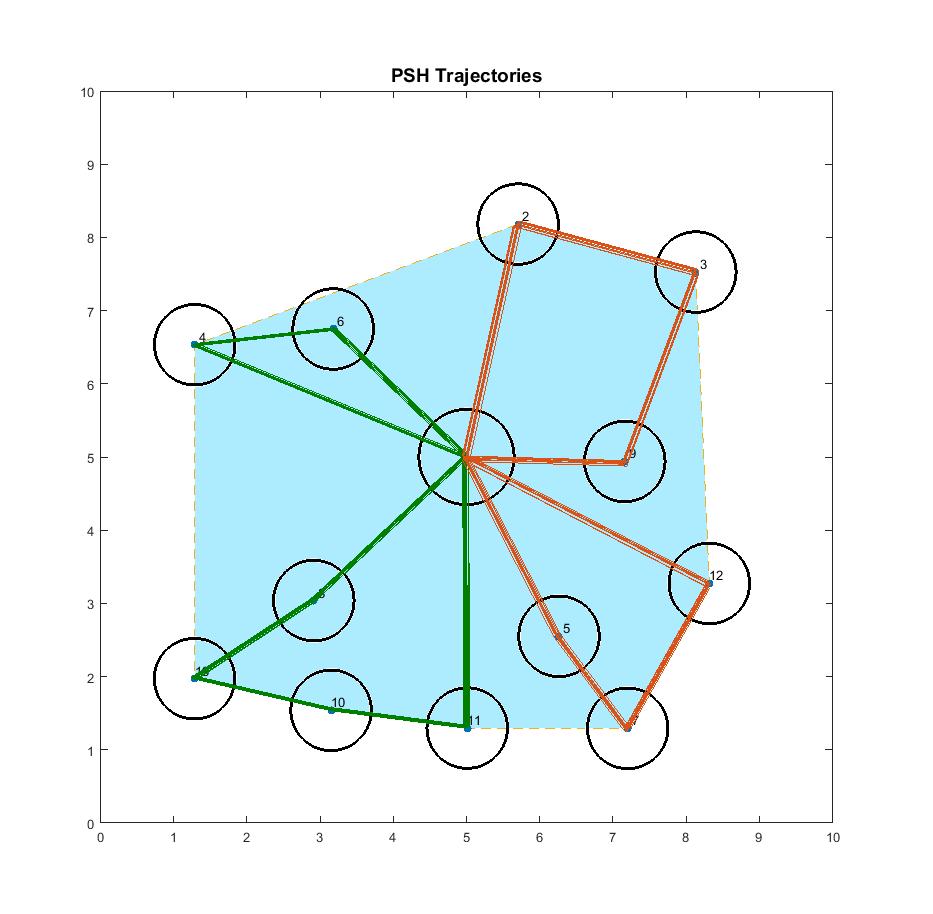
(a) PSH Sequences for case III

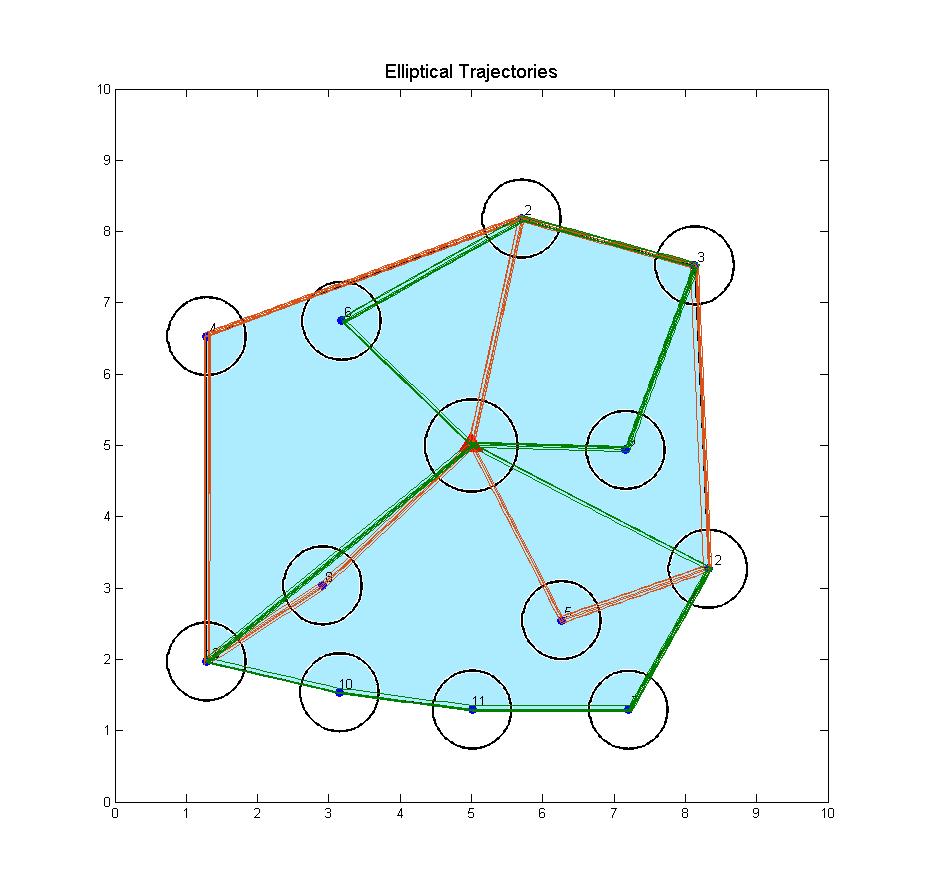
(b) Elliptical Sequences for case III

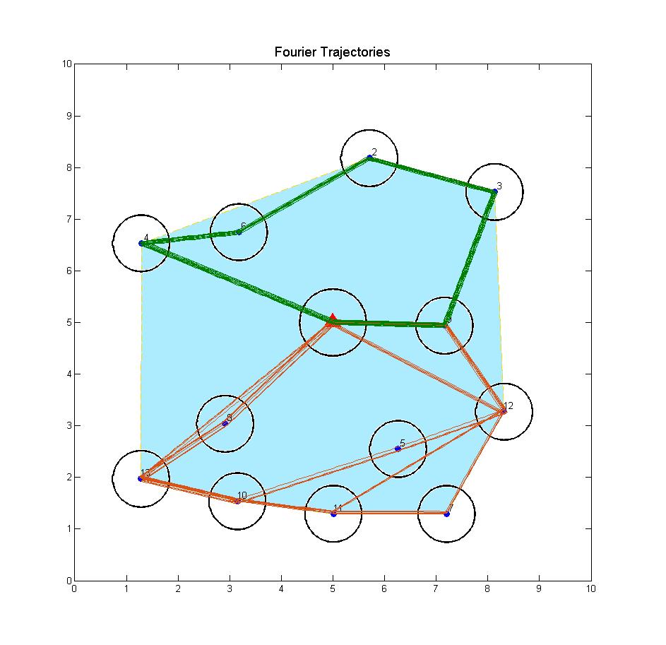
(c) Fourier Sequences for case III

Figure 8: Sequence Comparison

TABLE V: Result Comparison with PSH for Case II

Method	$J_{1}^{*}$	$-J_{2}^{*}$
PSH Sequence	0.023	-0.22
Elliptical Sequence	0.027	-0.21
Fourier Sequence	0.024	-0.21

TABLE VI: Result Comparison with PSH for Case III

Method	$J_{1}^{*}$	$-J_{2}^{*}$
PSH Sequence	0.0257	-0.21
Elliptical Sequence	0.0304	-0.199
Fourier Sequence	0.0212	-0.21

VI Conclusions

We have demonstrated a new event-driven methodology for on-line trajectory optimization with application in the data harvesting problem. We proposed a new performance measure that addresses the event excitation problem in event-driven controllers. The proposed optimal control problem is then formulated as a parametric trajectory optimization utilizing general function families which can be subsequently optimized on line through the use of Infinitesimal Perturbation Analysis (IPA). Several numerical results are provided for the case of elliptical and Fourier series trajectories and some properties of the solution are identified, including robustness with respect to the stochastic data generation processes and scalability in the size of the event set characterizing the underlying hybrid dynamic system.

Although the proposed methodology is focused on applying the event-driven optimization approach to the data harvesting problem, it should be noted that the new metric which was introduced in [25] to ensure event excitation allows us to generalize the methodology to other applications as well. The new metric introduces a potential field or density map over the entire mission space. This can viewed as a probability distribution of potential targets in problems where the exact locations of targets are unknown. Used as a prior distribution, it can be improved while the agents move within the mission space and gather more information. In addition, this density can be dynamically changing if the targets are moving and their location changes with time assuming some prior information about the target paths. This provides a tool to apply agent trajectory optimization in a much broader range of problems tracking moving points of interest.

Appendix A Proofs

Proposition 19:

Proof:

Fixing $X_{i}(t)=x_{i}(t)$, from (18) we have

$$\int_{\mathcal{C}}R(w,t) =\int_{\mathcal{C}}\sum_{i=1}^{M}\frac{\alpha_{i}x_{i}(t)}{d_{i}^{+}(w)}dw=\sum_{i=1}^{M}\alpha_{i}\int_{\mathcal{C}}\frac{x_{i}(t)}{d_{i}^{+}(w)}dw$$

To evaluate $\int_{\mathcal{C}}\frac{x_{i}(t)}{d_{i}^{+}(w)}$ for each target $i$, we first look at the case of a single target in a $2D$ space and temporarily replace $\mathcal{C}$ by a disk with radius $\Lambda$ around the target (black circle with radius $\Lambda$ in Fig. 9). We can now calculate the integral above using polar coordinates:

$$\int_{\mathcal{C}}\frac{x_{i}(t)}{d_{i}^{+}(w)}dw=\int_{0}^{2\pi}\int_{0}^{\Lambda}\frac{x_{i}(t)}{\max(r_{i},r)}drd\theta$$

$$=\int_{0}^{2\pi}\int_{0}^{r_{i}}\frac{x_{i}(t)}{r_{i}}drd\theta+\int_{0}^{2\pi}\int_{r_{i}}^{\Lambda}\frac{x_{i}(t)}{r}drd\theta$$

$$=x_{i}(t)\big{[}2\pi\big{(}1+\log(\frac{\Lambda}{r_{i}})\big{)}\big{]}$$

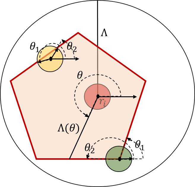
Figure 9: One Target $R(w,t)$ Calculation

Since $\mathcal{C}$ is actually the convex hull of all targets, we will use the same idea to calculate $\int_{\mathcal{C}}\frac{x_{i}(t)}{d_{i}^{+}(w)}dw$ where $\mathcal{C}$ is the convex hull by considering three separate cases depending on the target location.

1. Target $i$ and $C(w_{i})$ are completely in the interior of $\mathcal{C}$: This is shown in Fig. 9 for the red target. Using the same polar coordinate for each $\theta$, we define $\Lambda(\theta)$ to be the distance of the target to the edge of $\mathcal{C}$ in the direction of $\theta$ and get:

$$\int_{\mathcal{C}}\frac{x_{i}(t)}{d_{i}^{+}(w)}dw=\int_{0}^{2\pi}\int_{0}^{\Lambda(\theta)}\frac{x_{i}(t)}{d_{i}^{+}(r,\theta)}drd\theta$$

$$=\int_{0}^{2\pi}\int_{0}^{r_{i}}\frac{x_{i}(t)}{r_{i}}drd\theta+\int_{0}^{2\pi}\int_{r_{i}}^{\Lambda(\theta)}\frac{x_{i}(t)}{r}drd\theta$$

$$=x_{i}(t)\big{[}2\pi+\int_{0}^{2\pi}\log(\frac{\Lambda(\theta)}{r_{i}})d\theta\big{]}$$ (50)

The second part in (50) is calculated knowing that $\Lambda(\theta)\geq r_{i}$. This means $\log(\frac{\Lambda(\theta)}{r_{i}})>0$ and the term in brackets is positive. We can then define $c_{i}$ in (19) as

$$c_{i}=\alpha_{i}\big{[}2\pi+\int_{0}^{2\pi}\log(\frac{\Lambda(\theta)}{r_{i}})d\theta\big{]}$$ (51)

2. Target $i$ is on an edge of $\mathcal{C}$: This is shown in Fig. 9 for the green target. Since $C(w_{i})$ is not entirely contained within $\mathcal{C}$, we have

$$\int_{\mathcal{C}}\frac{x_{i}(t)}{d_{i}^{+}(w)}dw=\int_{0}^{2\pi}\int_{0}^{\Lambda(\theta)}\frac{x_{i}(t)}{d_{i}^{+}(r,\theta)}drd\theta$$

$$=\int_{\theta_{1}}^{\theta_{2}}\int_{0}^{r_{i}}\frac{x_{i}(t)}{r_{i}}drd\theta+\int_{\theta_{1}}^{\theta_{2}}\int_{r_{i}}^{\Lambda(\theta)}\frac{x_{i}(t)}{r}drd\theta$$

$$=x_{i}(t)\big{[}\theta_{2}-\theta_{1}+\int_{\theta_{1}}^{\theta_{2}}\log(\frac{\Lambda(\theta)}{r_{i}})d\theta\big{]}$$ (52)

The second part in (52) is calculated knowing that for $\theta\in[\theta_{1}~{}\theta_{2}]$ we have $\Lambda(\theta)\geq r_{i}$. Therefore, $\log(\frac{\Lambda(\theta)}{r_{i}})>0$ and by definition $\theta_{2}-\theta_{1}>0$ so that the term in brackets is positive. We can then define $c_{i}$ in (19) as

$$c_{i}=\alpha_{i}\big{[}\theta_{2}-\theta_{1}+\int_{\theta_{1}}^{\theta_{2}}\log(\frac{\Lambda(\theta)}{r_{i}})d\theta\big{]}$$ (53)

3. Target $i$ is in the interior of $\mathcal{C}$ but $C(w_{i})$ is not completely in the interior of $\mathcal{C}$: This is the case of the yellow target in Fig. 9. Carrying out the integration for the appropriate limits, since $C(w_{i})$ is not fully contained in $\mathcal{C}$:

$$\int_{\mathcal{C}}\frac{x_{i}(t)}{d_{i}^{+}(w)}dw=\int_{0}^{2\pi}\int_{0}^{\Lambda(\theta)}\frac{x_{i}(t)}{d_{i}^{+}(r,\theta)}drd\theta$$

$$=\int_{0}^{2\pi}\int_{0}^{r(\theta)}\frac{x_{i}(t)}{r_{i}}drd\theta+\int_{\theta_{1}}^{\theta_{2}}\int_{r_{i}}^{\Lambda(\theta)}\frac{x_{i}(t)}{r}drd\theta$$

$$=x_{i}(t)\big{[}\int_{0}^{2\pi}\frac{r(\theta)}{r_{i}}d\theta+\int_{\theta_{1}}^{\theta_{2}}\log(\frac{\Lambda(\theta)}{r_{i}})d\theta\big{]}$$ (54)

Here, $\Lambda(\theta)$ is only defined for $\theta\in[\theta_{1}~{}\theta_{2}]$ as shown in Fig. 9 for the yellow target. Again, since $\Lambda(\theta)\geq r_{i}$, it follows that $\log(\frac{\Lambda(\theta)}{r_{i}})>0$ and with $r(\theta)>0$ the term in brackets above is positive. We can define $c_{i}$ in (19) as

$$c_{i}=\alpha_{i}\big{[}\int_{0}^{2\pi}\frac{r(\theta)}{r_{i}}d\theta+\int_{\theta_{1}}^{\theta_{2}}\log(\frac{\Lambda(\theta)}{r_{i}})d\theta\big{]}$$ (55)

∎

Appendix B Elliptical Trajectories

In order to calculate the IPA derivatives we need the derivatives of state variable associated with agents with respect to all entries in the parameter vector $\Theta_{j}=[A_{j},B_{j},a_{j},b_{j},\phi_{j}]$ for all agents $j$. These derivatives do not depend on the events in the system, since the agent trajectories are fixed at each iteration. For now we assume $\mathcal{E}_{j}=1$ for all $j=1,\dots,N$ hence, we drop the superscript. We have:

$$\frac{\partial s_{j}^{x}}{\partial A_{j}}=1,\qquad\frac{\partial s_{j}^{x}}{\partial B_{j}}=0$$ (56)

$$\frac{\partial s_{j}^{x}}{\partial a_{j}}=\cos\rho_{j}(t)\cos\phi_{j},\qquad\frac{\partial s_{j}^{x}}{\partial b_{j}}=-\sin\rho_{j}(t)\sin\phi_{j}$$ (57)

$$\frac{\partial s_{j}^{x}}{\partial\phi_{j}}=-a_{j}\cos\rho_{j}(t)\sin\phi_{j}-b_{j}\sin\rho_{j}(t)\cos\phi_{j}$$ (58)

$$\frac{\partial s_{j}^{y}}{\partial A_{j}}=0,\qquad\frac{\partial s_{j}^{y}}{\partial B_{j}}=1$$ (59)

$$\frac{\partial s_{j}^{y}}{\partial a_{j}}=\cos\rho_{j}(t)\sin\phi_{j},\qquad\frac{\partial s_{j}^{y}}{\partial b_{j}}=\sin\rho_{j}(t)\cos\phi_{j}$$ (60)

$$\frac{\partial s_{j}^{y}}{\partial\phi_{j}}=a_{j}\cos\rho_{j}(t)\cos\phi_{j}-b_{j}\sin\rho_{j}(t)\sin\phi_{j}$$ (61)

The time derivative of the position state variables are calculated as follows:

The gradient of the last term in the $J_{e}$ in (47) needs to be calculated separately. We have for $j\neq l$, $\frac{\partial\mathcal{C}_{j}}{\partial\Theta_{l}}=0$ and for $j=l$:

$$\frac{\partial\mathcal{C}_{j}}{\partial A_{j}}=2\mathcal{C}_{j}\big{(}-\cos^{2}\phi_{j}\frac{\partial f_{j}^{1}}{\partial A_{j}}-\sin^{2}\phi_{j}\frac{\partial f_{j}^{2}}{\partial A_{j}}-\sin 2\phi_{j}\frac{\partial f_{j}^{3}}{\partial A_{j}}\big{)}$$

$$\frac{\partial\mathcal{C}_{j}}{\partial B_{j}}=2\mathcal{C}_{j}\big{(}-\cos^{2}\phi_{j}\frac{\partial f_{j}^{1}}{\partial B_{j}}-\sin^{2}\phi_{j}\frac{\partial f_{j}^{2}}{\partial B_{j}}-\sin 2\phi_{j}\frac{\partial f_{j}^{3}}{\partial B_{j}}\big{)}$$

$$\frac{\partial\mathcal{C}_{j}}{\partial a_{j}}=2\mathcal{C}_{j}\big{(}-\cos^{2}\phi_{j}\frac{\partial f_{j}^{1}}{\partial a_{j}}-\sin^{2}\phi_{j}\frac{\partial f_{j}^{2}}{\partial a_{j}}-\sin 2\phi_{j}\frac{\partial f_{j}^{3}}{\partial a_{j}}\big{)}$$

$$\frac{\partial\mathcal{C}_{j}}{\partial b_{j}}=2\mathcal{C}_{j}\big{(}-\cos^{2}\phi_{j}\frac{\partial f_{j}^{1}}{\partial b_{j}}-\sin^{2}\phi_{j}\frac{\partial f_{j}^{2}}{\partial b_{j}}-\sin 2\phi_{j}\frac{\partial f_{j}^{3}}{\partial b_{j}}\big{)}$$

$$\frac{\partial\mathcal{C}_{j}}{\partial\phi_{j}}=2\mathcal{C}_{j}\big{(}(f_{j}^{1}-f_{j}^{2})\sin 2\phi_{j}-2f_{j}^{3}\cos 2\phi_{j}\big{)}$$

where

$$\begin{split}\frac{\partial f_{j}^{1}}{\partial A_{j}}&=-2\Big{(}\frac{w_{\!{}_{B}}^{x}-A_{j}}{a_{j}^{2}}\Big{)},\quad\frac{\partial f_{j}^{1}}{\partial B_{j}}=-2\Big{(}\frac{w_{\!{}_{B}}^{y}-B_{j}}{b_{j}^{2}}\Big{)}\\ \frac{\partial f_{j}^{1}}{\partial a_{j}}&=-2\Big{(}\frac{(w_{\!{}_{B}}^{x}-A_{j})^{2}}{a_{j}^{3}}\Big{)},\quad\frac{\partial f_{j}^{1}}{\partial b_{j}}=-2\Big{(}\frac{(w_{\!{}_{B}}^{y}-B_{j})^{2}}{b_{j}^{3}}\Big{)}\\ &\end{split}$$

$$\begin{split}\frac{\partial f_{j}^{2}}{\partial A_{j}}&=-2\Big{(}\frac{w_{\!{}_{B}}^{x}-A_{j}}{b_{j}^{2}}\Big{)},~{}\frac{\partial f_{j}^{2}}{\partial B_{j}}=-2\Big{(}\frac{w_{\!{}_{B}}^{y}-B_{j}}{a_{j}^{2}}\Big{)}\\ \frac{\partial f_{j}^{2}}{\partial a_{j}}&=-2\Big{(}\frac{(w_{\!{}_{B}}^{y}-B_{j})^{2}}{a_{j}^{3}}\Big{)},~{}\frac{\partial f_{j}^{2}}{\partial b_{j}}=-2\Big{(}\frac{(w_{\!{}_{B}}^{x}-A_{j})^{2}}{b_{j}^{3}}\Big{)}\\ &\end{split}$$

$$\begin{split}\frac{\partial f_{j}^{3}}{\partial A_{j}}&=-\Big{(}\frac{(b_{j}^{2}-a_{j}^{2})(w_{\!{}_{B}}^{y}-B_{j})}{a_{j}^{2}b_{j}^{2}}\Big{)}\\ \frac{\partial f_{j}^{3}}{\partial B_{j}}&=-\Big{(}\frac{(b_{j}^{2}-a_{j}^{2})(w_{\!{}_{B}}^{x}-A_{j})}{a_{j}^{2}b_{j}^{2}}\Big{)}\end{split}$$

$$\begin{split}\frac{\partial f_{j}^{3}}{\partial a_{j}}&=-2\Big{(}\frac{(w_{\!{}_{B}}^{x}-A_{j})(w_{\!{}_{B}}^{y}-B_{j})}{a_{j}^{3}}\Big{)}\\ \frac{\partial f_{j}^{3}}{\partial b_{j}}&=2\Big{(}\frac{(w_{\!{}_{B}}^{x}-A_{j})(w_{\!{}_{B}}^{y}-B_{j})}{b_{j}^{3}}\Big{)}\end{split}$$

Appendix C Fourier Series Trajectories

In the Fourier parametric trajectories the agent state derivative is calculated as follows. The parameter vector is $\Theta_{j}=[f_{j}^{x},a_{0,j},\ldots,a_{\Gamma_{j}^{x}},b_{0,j},\ldots,b_{\Gamma_{j}^{y}},\phi_{1,j},\ldots,\phi_{\Gamma_{j}^{x}},\xi_{1,j},\ldots,\xi_{\Gamma_{j}^{y}}]$. Thus, we have:

$$\frac{\partial s_{j}^{x}}{\partial a_{0,j}}=1,\qquad\frac{\partial s_{j}^{x}}{\partial b_{0,j}}=0$$ (64)

$$\frac{\partial s_{j}^{x}}{\partial a_{n,j}}=\sin(2\pi nf_{j}^{x}\rho_{j}(t)+\phi_{n,j}^{x}),\qquad\frac{\partial s_{j}^{x}}{\partial b_{n,j}}=0$$ (65)

$$\frac{\partial s_{j}^{x}}{\partial\phi_{n,j}^{x}}=a_{n,j}\cos(2\pi nf_{j}^{x}\rho_{j}(t)+\phi_{n,j}^{x})\qquad\frac{\partial s_{j}^{x}}{\partial\phi_{n,j}^{y}}=0$$ (66)

$$\frac{\partial s_{j}^{x}}{\partial f_{j}^{x}}=2\pi\rho_{j}(t)\displaystyle\sum_{n=1}^{\Gamma_{j}^{x}}a_{n,j}n\cos(2\pi nf_{j}^{x}\rho_{j}(t)+\phi_{n,j}^{x}),$$ (67)

$$\frac{\partial s_{j}^{y}}{\partial b_{0,j}}=1,\qquad\frac{\partial s_{j}^{y}}{\partial a_{0,j}}=0$$ (68)

$$\frac{\partial s_{j}^{y}}{\partial b_{n,j}}=\sin(2\pi nf_{j}^{y}\rho_{j}(t)+\phi_{n,j}^{y}),\qquad\frac{\partial s_{j}^{y}}{\partial a_{n,j}}=0$$ (69)

$$\frac{\partial s_{j}^{y}}{\partial\phi_{n,j}^{y}}=b_{n,j}\cos(2\pi nf_{j}^{y}\rho_{j}(t)+\phi_{n,j}^{y})\qquad\frac{\partial s_{j}^{y}}{\partial\phi_{n,j}^{x}}=0$$ (70)

$$\frac{\partial s_{j}^{y}}{\partial f_{j}^{x}}=0$$ (71)

The time derivative of the position state variables are calculated as follows:

$$\dot{s}_{j}^{x}(t)=\dot{\rho}_{j}(t)\sum_{n=1}^{\Gamma_{j}^{x}}2\pi nf_{j}^{x}a_{n,j}\cos(2\pi nf_{j}^{x}\rho_{j}(t)+\phi_{n,j}^{x}),$$ (72)

$$\dot{s}_{j}^{y}(t)=\dot{\rho}_{j}(t)\sum_{n=1}^{\Gamma_{j}^{y}}2\pi nf_{j}^{y}b_{n,j}\cos(2\pi nf_{j}^{y}\rho_{j}(t)+\phi_{n,j}^{y}),$$ (73)

Appendix D IPA events and derivatives

In this section, we derive all event time derivatives and state derivatives with respect to the controllable parameter $\Theta$ for each event by applying the IPA equations.
1. Event $\xi_{i}^{0}$: This event causes a transition from $X_{i}(t)>0$, $t<\tau_{k}$ to $X_{i}(t)=0$, $t\geq\tau_{k}$. The switching function is $g_{k}(\Theta,\mathbf{X})=X_{i}$ so $\frac{\partial g_{k}}{\partial X_{i}}=1$. From (39) and (5):

$$\begin{split}{\tau_{k}^{\prime}}&=-\Big{(}\frac{\partial g_{k}}{\partial X_{i}}f_{k}(\tau_{k}^{-})\Big{)}^{-1}\Big{(}g^{\prime}_{k}+\frac{\partial g_{k}}{\partial X_{i}}{X_{i}^{\prime}(\tau_{k}^{-})}\Big{)}\\ &=-\frac{X_{i}^{\prime}(\tau_{k}^{-})}{\sigma_{i}(\tau_{k})-\mu_{ij}p_{ij}(\tau_{k})}\end{split}$$ (74)

where agent $j$ is the one connected to $i$ at $t=\tau_{k}$ and we have used the assumption that two events occur at the same time w.p. $0$, hence $\sigma_{i}(\tau_{k}^{-})=\sigma_{i}(\tau_{k})$. From (40)-(41), since $\dot{X}_{i}(t)=0$, for $\tau_{k}\leq t<\tau_{k+1}$:

$$\frac{d}{dt}X_{i}^{\prime}(t)=\frac{\partial\dot{X}_{i}(t)}{\partial X_{i}(t)}X_{i}^{\prime}(t)+{\dot{X}_{i}^{\prime}(t)}=0$$ (75)

$$\begin{split}&X_{i}^{\prime}(\tau_{k}^{+})=X_{i}^{\prime}(\tau_{k}^{-})+\Big{[}\Big{(}\sigma_{i}(\tau_{k})-\mu_{ij}p_{ij}(\tau_{k})\Big{)}-0\Big{]}{\tau_{k}}^{\prime}\\ &=X_{i}^{\prime}(\tau_{k}^{-})-\frac{X_{i}^{\prime}(\tau_{k}^{-})\Big{(}\sigma_{i}(\tau_{k})-\mu_{ij}p_{ij}(\tau_{k})\Big{)}}{\sigma_{i}(\tau_{k})-\mu_{ij}p_{ij}(\tau_{k})}=0\end{split}$$ (76)

For $X_{r}(t)$, $r\neq i$, the dynamics of $X_{r}(t)$ in (5) are unaffected and we have:

$$X_{r}^{\prime}(\tau_{k}^{+})=X_{r}^{\prime}(\tau_{k}^{-})$$ (77)

If $X_{r}(\tau_{k})>0$ and agent $l$ is connected to it, then

$$\begin{split}&\frac{d}{dt}X_{r}^{\prime}(t)=\frac{\partial\dot{X}_{r}(t)}{\partial X_{r}(t)}X_{r}^{\prime}(t)+{\dot{X}_{r}^{\prime}(t)}\\ &=\sigma_{r}^{\prime}(t)-\mu_{rl}p^{\prime}_{rl}(\tau_{k})=-\mu_{rl}p_{rl}^{\prime}(t)\end{split}$$ (78)

and if ${X}_{r}(t)=0$ in $[\tau_{k},\tau_{k+1}]$ or if no agents are connected to $i$, then $\frac{d}{dt}X_{r}^{\prime}(t)=0$.
For $Y_{r}(t)$, $r=1,\dots,M$, the dynamics of $Y_{r}(t)$ in (8) are not affected by the event $\xi_{i}^{0}$ at $\tau_{k}$, hence

$$Y_{r}^{\prime}(\tau_{k}^{+})=Y_{r}^{\prime}(\tau_{k}^{-})$$ (79)

and since $\dot{Y}_{r}(t)=\beta_{r}(t)$, for $\tau_{k}\leq t<\tau_{k+1}$:

$$\frac{d}{dt}Y_{r}^{\prime}(t)=\frac{\partial\dot{Y}_{r}(t)}{\partial Y_{r}(t)}Y_{r}^{\prime}(t)+{\dot{Y}_{r}^{\prime}(t)}=\beta_{r}^{\prime}(t)$$ (80)

For $Z_{ij}(t)$, we must have $Z_{ij}(\tau_{k})>0$ since $X_{i}(\tau_{k}^{-})>0$, hence $\tilde{\mu}_{ij}(\tau_{k}^{-})>0$ and from (41):

$$\begin{split}&Z_{ij}^{\prime}(\tau_{k}^{+})=Z_{ij}^{\prime}(\tau_{k}^{-})+\Big{[}\dot{Z}_{ij}(\tau_{k}^{-})-\dot{Z}_{ij}(\tau_{k}^{+})\Big{]}\tau_{k}^{\prime}\\ &=Z_{ij}^{\prime}(\tau_{k}^{-})+\Big{[}\tilde{\mu}_{ij}(\tau_{k}^{-})-\tilde{\mu}_{ij}(\tau_{k}^{+})\Big{]}p_{ij}(\tau_{k})\tau_{k}^{\prime}\end{split}$$ (81)

Since $X_{i}(\tau_{k}^{-})>0$, from (6) we have $\tilde{\mu}_{ij}(\tau_{k}^{-})=\mu_{ij}$. At $\tau_{k}^{+}$, $j$ remains connected to target $i$ with $\tilde{\mu}_{ij}(\tau_{k}^{+})=\sigma_{i}(\tau_{k}^{+})/p_{ij}(\tau_{k})=\sigma_{i}(\tau_{k})/p_{ij}(\tau_{k})$ and we get

From (40) for $\tau_{k}\leq t<\tau_{k+1}$:

$$\begin{split}&\frac{d}{dt}Z_{ij}^{\prime}(t)=\frac{\partial\dot{Z}_{ij}(t)}{\partial Z_{ij}(t)}Z_{ij}^{\prime}(t)+\dot{Z}^{\prime}_{ij}(t)\\ &=\dot{Z}^{\prime}_{ij}(t)=\Big{(}\tilde{\mu}_{ij}(t)P^{\prime}_{ij}(t)-\beta_{ij}P^{\prime}_{\!{}_{Bj}}(t)\Big{)}\end{split}$$ (83)

Since $\tilde{\mu}_{ij}(t)=\sigma_{i}(t)/p_{ij}(t)$ for the agent which remains connected to target $i$ after this event, it follows that $\frac{\partial}{\partial\Theta}[\tilde{\mu}_{ij}(t)p_{ij}(t)]=0$. Moreover, $p_{\!{}_{Bj}}(t)=0$ by our assumption that agents cannot be within range of the base and targets at the same time and we get

$$\frac{d}{dt}Z_{ij}^{\prime}(t)=0$$ (84)

Otherwise, for $r\neq j$, we have $\tilde{\mu}_{ir}(t)=0$ and we get:

$$\frac{d}{dt}Z_{ir}^{\prime}(t)=-\beta_{ir}p_{\!{}_{Br}}^{\prime}(t)$$ (85)

Finally, for $Z_{rj}(t)$, $r\neq i$ we have $Z_{rj}^{\prime}(\tau_{k}^{+})=Z_{rj}^{\prime}(\tau_{k}^{-})$. If $Z_{rj}(t)=0$ in $[\tau_{k},\tau_{k+1})$, then $\frac{d}{dt}Z_{rj}^{\prime}(t)=0$. Otherwise, we get $\frac{d}{dt}Z_{rj}^{\prime}(t)$ from (83) with $i$ replaced by $r$.
2. Event $\xi_{i}^{+}$: This event causes a transition from $X_{i}(t)=0$, $t\leq\tau_{k}$ to $X_{i}(t)>0$, $t>\tau_{k}$. Note that this transition can occur as an exogenous event when an empty queue $X_{i}(t)$ gets a new arrival in which case we simply have $\tau_{k}^{\prime}=0$ since the exogenous event is independent of the controllable parameters. In the endogenous case, however, we have the switching function $g_{k}(\Theta,\mathbf{X})=\sigma_{i}(t)-\mu_{ij}p_{ij}(t)$ in which agent $j$ is connected to target $i$ at $t=\tau_{k}$. Assuming $s_{j}^{\prime}(t)=\big{[}\frac{\partial s_{j}^{x}}{\partial\Theta}~{}\frac{\partial s_{j}^{y}}{\partial\Theta}\big{]}^{\top}$ and $\dot{s}_{j}=[\dot{s}_{j}^{x}~{}\dot{s}_{j}^{y}]^{\top}$, from (39):

$$\begin{split}{\tau_{k}}^{\prime}&=-\Big{(}\frac{\partial g_{k}}{\partial s_{j}}s_{j}^{\prime}(\tau_{k})\Big{)}\Big{(}{g_{k}^{\prime}\dot{s}_{j}(\tau_{k})}\Big{)}^{-1}\end{split}$$ (86)

At $\tau_{k}$ we have $\sigma_{i}(\tau_{k})=\mu_{ij}p_{ij}(\tau_{k})$. Therefore from (41):

$$\begin{split}&X_{i}^{\prime}(\tau_{k}^{+})=X_{i}^{\prime}(\tau_{k}^{-})+[\dot{X}_{i}(\tau_{k}^{-})-\dot{X}_{i}(\tau_{k}^{+})]{\tau_{k}}^{\prime}\\ &=X_{i}^{\prime}(\tau_{k}^{-})+\Big{(}0-\sigma_{i}(\tau_{k})+\mu_{ij}p_{ij}(\tau_{k})\Big{)}{\tau_{k}}^{\prime}=X_{i}^{\prime}(\tau_{k}^{-})\end{split}$$ (87)

Having $X_{i}(t)>0$ in $[\tau_{k},\tau_{k+1})$ we know $\dot{X}_{i}(t)=\sigma_{i}(t)-\mu_{ij}p_{ij}(t)$ therefor, we can get $\frac{d}{dt}X_{i}^{\prime}(t)$ from (78) with $r$ and $l$ replaced by $i$ and $j$. For $X_{r}(t)$, $r\neq i$, if $X_{r}(\tau_{k})>0$ and agent $l$ is connected to $r$ then $\dot{X}_{r}(\tau_{k})=\sigma_{r}(\tau_{k})-\mu_{rl}p_{rl}(\tau_{k})$, therefor, we get $X^{\prime}_{r}(\tau_{k}^{+})$ from (77) while in $[\tau_{k},\tau_{k+1})$ we have $\frac{d}{dt}X^{\prime}_{r}(t)$ from (78). If $X_{r}(\tau_{k})=0$ or if no agent is connected to target $r$, $\dot{X}_{r}(\tau_{k})=0$. Thus, $X^{\prime}_{r}(\tau_{k}^{+})=X^{\prime}_{r}(\tau_{k}^{-})$ and $\frac{d}{dt}X^{\prime}_{r}(t)=0$.
For $Y_{r}(t)$, $r=1,\dots,M$ the dynamics of $Y_{r}(t)$ in (8) are not affected by the event at $\tau_{k}$ hence, we can get $Y^{\prime}_{r}(\tau_{k}^{+})$ and $\frac{d}{dt}Y^{\prime}_{r}(t)$ in $[\tau_{k},\tau_{k+1})$ from (79) and (80) respectively.
For $Z_{ij}(t)$ assuming agent $j$ is the one connected to target $i$, we have:

$$\begin{split}&Z^{\prime}_{ij}(\tau_{k}^{+})=Z^{\prime}_{ij}(\tau_{k}^{-})+\Big{[}\dot{Z}_{ij}(\tau_{k}^{-})-\dot{Z}_{ij}(\tau_{k}^{+})\Big{]}\tau^{\prime}_{k}\\ &=Z^{\prime}_{ij}(\tau_{k}^{-})+\Big{[}\tilde{\mu}_{ij}(\tau_{k}^{-})-\tilde{\mu}_{ij}(\tau_{k}^{+})\Big{]}p_{ij}(\tau_{k})\tau^{\prime}_{k}=Z^{\prime}_{ij}(\tau_{k}^{-})\end{split}$$ (88)

In the above equation, $\tilde{\mu}_{ij}(\tau_{k}^{+})=\mu_{ij}$ because $X_{i}(\tau_{k}^{+})>0$. Also, $\mu_{ij}p_{ij}(\tau_{k})=\sigma_{i}(\tau_{k})$ and $\tilde{\mu}_{ij}(\tau_{k}^{-})=\frac{\sigma_{i}(\tau_{k})}{p_{ij}(\tau_{k})}$ results in $\tilde{\mu}_{ij}(\tau_{k}^{+})=\mu_{ij}$. For $Z_{il}(t)$, $l\neq j$ , agent $l$ cannot be connected to target $i$ at $\tau_{k}$ so we have, $Z^{\prime}_{il}(\tau_{k}^{+})=Z^{\prime}_{il}(\tau_{k}^{-})$ and $\frac{d}{dt}Z^{\prime}_{il}(t)=0$ in $[\tau_{k},\tau_{k+1})$. For $Z_{rl}(t)$ ,$r\neq i$ and $l\neq j$ using the assumption that two events occur at the same time w.p. 0, the dynamics of $Z_{rl}(t)$ are not affected at $\tau_{k}$, hence we get $\frac{d}{dt}Z^{\prime}_{rl}(t)$ from (83) for $i$ and $j$ replaced by $r$ and $l$.
3. Event $\zeta_{ij}^{0}$: This event causes a transition from $Z_{ij}(t)>0$ for $t<\tau_{k}$ to $Z_{ij}(t)=0$ for $t\geq\tau_{k}$. The switching function is $g_{k}(\Theta,\mathbf{X})=Z_{ij}(t)$ so $\frac{\partial g_{k}}{\partial Z_{ij}}=1$. From (39):

$$\begin{split}&{\tau_{k}}^{\prime}=-\Big{(}\frac{\partial g_{k}}{\partial Z_{ij}}f_{k}(\tau^{-}_{k})\Big{)}^{-1}\Big{(}g^{\prime}_{k}+\frac{\partial g_{k}}{\partial Z_{ij}}{Z_{ij}^{\prime}(\tau^{-}_{k})}\Big{)}\\ &=-\frac{Z_{ij}^{\prime}(\tau^{-}_{k})}{\tilde{\mu}_{ij}(\tau^{-}_{k})p_{ij}(\tau^{-}_{k})-\beta_{ij}p_{\!{}_{Bj}}(\tau^{-}_{k})}=\frac{Z_{ij}^{\prime}(\tau^{-}_{k})}{\beta_{ij}p_{\!{}_{Bj}}(\tau_{k})}\end{split}$$ (89)

Since $Z_{ij}(t)$ is being emptied at $\tau_{k}$, by the assumption that agents can not be in range with the base and targets at the same time, we have $p_{ij}(\tau_{k})=0$. Then from (41):

$$\begin{split}&Z^{\prime}_{ij}(\tau_{k}^{+})=Z^{\prime}_{ij}(\tau_{k}^{-})+\Big{[}-\beta_{ij}p_{\!{}_{Bj}}(\tau_{k})-0\Big{]}{\tau_{k}}^{\prime}\\ &=Z^{\prime}_{ij}(\tau_{k}^{-})-\Big{[}\beta_{ij}p_{\!{}_{Bj}}(\tau_{k})\Big{]}\frac{Z_{ij}^{\prime}(\tau^{-}_{k})}{\beta_{ij}p_{\!{}_{Bj}}(\tau_{k})}=0\end{split}$$ (90)

Since $\dot{Z}_{ij}(t)=0$ in $[\tau_{k},\tau_{k+1})$:

$$\frac{d}{dt}Z^{\prime}_{ij}(t)=\frac{\partial\dot{Z}_{ij}(t)}{\partial Z_{ij}(t)}Z^{\prime}_{ij}(t)+\dot{Z}^{\prime}_{ij}(t)=0$$ (91)

For $Z_{rl}(t)$, $r\neq i$ or $l\neq j$, the dynamics in (7) are not affected at $\tau_{k}$, hence:

$$Z^{\prime}_{rl}(\tau_{k}^{+})=Z^{\prime}_{rl}(\tau_{k}^{-})$$ (92)

if $Z_{rl}(\tau_{k})>0$, the value for $\frac{d}{dt}Z^{\prime}_{rl}(t)$ is calculated by (83) with $r$ and $l$ replacing $i$ and $j$ respectively. If $Z_{rl}(\tau_{k})=0$ then $\frac{d}{dt}Z^{\prime}_{rl}(t)=0$.
For $Y_{i}(t)$ we have $\beta_{i}(\tau_{k}^{+})=0$ since the agent has emptied its queue, hence:

$$\begin{split}&Y^{\prime}_{i}(\tau_{k}^{+})=Y^{\prime}_{i}(\tau_{k}^{-})+\Big{[}\dot{Y}_{i}(\tau_{k}^{-})-\dot{Y}_{i}(\tau_{k}^{+})\Big{]}\tau^{\prime}_{k}\\ &=Y^{\prime}_{i}(\tau_{k}^{-})+[\beta_{ij}p_{\!{}_{Bj}}(\tau_{k})-0]\frac{Z_{ij}^{\prime}(\tau^{-}_{k})}{\beta_{ij}p_{\!{}_{Bj}}(\tau_{k})}\\ &=Y^{\prime}_{i}(\tau_{k}^{-})+Z_{ij}^{\prime}(\tau^{-}_{k})\end{split}$$ (93)

In $[\tau_{k},\tau_{k+1})$ we can get $\frac{d}{dt}Y^{\prime}_{i}(t)=0$. For $Y_{r}(t)$, $r\neq i$ the dynamics of $Y_{r}(t)$ in (8) are not affected by the event at $\tau_{k}$ hence, $Y^{\prime}_{r}(\tau_{k}^{+})$ and $\frac{d}{dt}Y^{\prime}_{r}(t)$ in $[\tau_{k},\tau_{k+1})$ are calculated from (79) and (80) respectively. The dynamics of $X_{r}(t)$, $r=1,\dots,M$ is are not affected at $\tau_{k}$ since the event at $\tau_{k}$ is happening at the base. We have $X_{r}^{\prime}(\tau_{k}^{+})=X_{r}^{\prime}(\tau_{k}^{-})$. If $X_{r}(\tau_{k})>0$ then we have $\frac{d}{dt}X^{\prime}_{r}(t)$ from (78) and if $X_{r}(\tau_{k})=0$ then $\frac{d}{dt}X^{\prime}_{r}(t)=0$ in $[\tau_{k},\tau_{k+1})$.
4. Event $\delta_{ij}^{+}$: This event causes a transition from $D^{+}_{ij}(t)=0$ for $t\leq\tau_{k}$ to $D^{+}_{ij}(t)>0$ for to $t>\tau_{k}$. It is the moment that agent $j$ leaves target $i$’s range. The switching function is $g_{k}(\Theta,\mathbf{X})=d_{ij}(t)-r_{ij}$ , from (39):

$${\tau_{k}}^{\prime}=-\frac{\partial d_{ij}}{\partial s_{j}}s_{j}^{\prime}(t)\Big{(}\frac{\partial d_{ij}}{\partial s_{j}}\dot{s}_{j}(\tau_{k})\Big{)}^{-1}$$ (94)

If agent $j$ was connected to target $i$ at $\tau_{k}$ then by leaving the target, it is possible that another agent $l$ which is within range with target $i$ connects to that target. This means $\dot{X}_{i}(\tau_{k}^{+})=\sigma_{i}(\tau_{k})-\mu_{il}p_{il}(\tau_{k})$ and $\dot{X}_{i}(\tau_{k}^{-})=\sigma_{i}(\tau_{k})-\mu_{ij}p_{ij}(\tau_{k})$, with $p_{ij}(\tau_{k})=0$, from (41) we have

$$X_{i}^{\prime}(\tau_{k}^{+})=X_{i}^{\prime}(\tau_{k}^{-})-\mu_{il}p_{il}(\tau_{k})\tau_{k}^{\prime}$$ (95)

If $X_{i}(\tau_{k})>0$, $\frac{d}{dt}X^{\prime}_{i}(t)$ in $[\tau_{k},\tau_{k+1})$ is as in (78) with $r$ replaced by $i$ and if $X_{i}(\tau_{k})=0$ then $\frac{d}{dt}X^{\prime}_{i}(t)=0$. On the other hand, if agent $j$ was not connected to target $i$ at $\tau_{k}$, we know that some $l\neq j$ is already connected to target $i$. This means agent $j$ leaving target $i$ cannot affect the dynamics of $X_{i}(t)$ so we have $X_{i}^{\prime}(\tau_{k}^{+})=X_{i}^{\prime}(\tau_{k}^{-})$ and $\frac{d}{dt}X_{i}^{\prime}(t)$ is calculated from (78) with $r$ replaced by $i$.
For $X_{r}(t)$, $r\neq i$ the dynamics in (5) are not affected by the event at $\tau_{k}$ hence, we get $X_{r}^{\prime}(\tau_{k}^{+})$ from (77). If $X_{r}(\tau_{k})>0$ the time derivative $\frac{d}{dt}X^{\prime}_{r}(t)$ in $[\tau_{k},\tau_{k+1})$ can be calculated from (78) and if $X_{r}(\tau_{k})=0$ then $\frac{d}{dt}X^{\prime}_{r}(t)=0$.
For $Y_{r}(t)$, $r=1,\ldots,,M$, the dynamics in (8) are not also affected by the event at $\tau_{k}$ hence, we get $Y_{r}(\tau_{k}^{+})$ from (79) and in $[\tau_{k},\tau_{k+1})$ the $\frac{d}{dt}Y^{\prime}_{r}(t)$ is calculated from (80).
For $Z_{ij}(t)$, the dynamics in (7) are not affect at $\tau_{k}$, regardless of the fact that agent $j$ is connected to target $i$ or not. We have $\dot{Z}_{ij}(\tau_{k}^{-})=\tilde{\mu}_{ij}(\tau_{k})p_{ij}(\tau_{k})$ with $p_{ij}(\tau_{k})=0$ and $\dot{Z}_{ij}(\tau_{k}^{+})=0$, hence from (41):

$$\begin{split}&Z^{\prime}_{ij}(\tau_{k}^{+})=Z^{\prime}_{ij}(\tau_{k}^{-})+\Big{[}\dot{Z}_{ij}(\tau_{k}^{-})-\dot{Z}_{ij}(\tau_{k}^{+})\Big{]}\tau^{\prime}_{k}\\ &=Z^{\prime}_{ij}(\tau_{k}^{-})+\tilde{\mu}_{ij}(\tau_{k})p_{ij}(\tau_{k})\tau^{\prime}_{k}=Z^{\prime}_{ij}(\tau_{k}^{-})\end{split}$$ (96)

and in $[\tau_{k},\tau_{k+1})$ , we have $\frac{d}{dt}Z^{\prime}_{ij}(t)=0$ using (83) knowing $p_{ij}(\tau_{k})=p_{\!{}_{Bj}}(\tau_{k})=0$. For $Z_{rl}(t)$, $r\neq i$ or $l\neq j$, the dynamics of $Z_{rl}(t)$ are not affected at $\tau_{k}$ hence (92) holds and in $[\tau_{k},\tau_{k+1})$ again we can use (83) with $i$ and $j$ replaced by $r$ and $l$.
5. Event $\delta_{ij}^{0}$: This event causes a transition from $D^{+}_{ij}(t)>0$ for $t<\tau_{k}$ to $D^{+}_{ij}(t)=0$ for to $t\geq\tau_{k}$. The event is the moment that agent $j$ enters target $i$’s range. The switching function is $g_{k}(\Theta,\mathbf{X})=d_{ij}(t)-r_{ij}$. From (39) we can get ${\tau_{k}}^{\prime}$ from (94). If no other agent is already connected to target $i$, agent $j$ connects to it. Otherwise, if another agent is already connected to target $i$, no connection is established. For $X_{i}(t)$, the dynamics in (5) are not affected in both cases, hence, (87) holds. If $X_{i}(t)>0$ in $[\tau_{k},\tau_{k+1})$ we calculate $\frac{d}{dt}X^{\prime}_{i}(t)$ using (78) with $l$ being the appropriate connected agent to target $i$. If $X_{i}(\tau_{k}^{-})=0$, $\frac{d}{dt}X^{\prime}_{i}(t)=0$. For $X_{r}(t)$, $r\neq i$ the dynamics in (5) are not affected by the event at $\tau_{k}$. Hence, we get $X_{r}^{\prime}(\tau_{k}^{+})$ from (77). If $X_{r}(\tau_{k})>0$ we calculate $\frac{d}{dt}X^{\prime}_{r}(t)$ from (78) with $i$ replaced by $r$ and if $X_{r}(\tau_{k})=0$ then $\frac{d}{dt}X^{\prime}_{r}(t)=0$.
For $Y_{r}(t)$, $r=1,\dots,M$ again the dynamics in (8) are not affected at $\tau_{k}$ so both (79) and (80) hold.
For $Z_{ij}(t)$, with agent $j$ being connected or not to target $i$ at $\tau_{k}$ the dynamics of $Z_{ij}(t)$ are unaffected at $\tau_{k}$, hence (92) holds for $i$ and $j$ and in $[\tau_{k},\tau_{k+1})$ the $\frac{d}{dt}Z^{\prime}_{ij}(t)$ is calculated through (83). For $Z_{rl}(t)$, $r\neq i$ or $l\neq j$ the dynamics are unaffected (92) holds again. In $[\tau_{k},\tau_{k+1})$, $\frac{d}{dt}Z^{\prime}_{rl}(t)$ is given through (83) with $i$ and $j$ replaced by $r$ and $l$.
6. Event $\Delta_{j}^{+}$: This event causes a transition from $D^{+}_{\!{Bj}}(t)=0$ for $t\leq\tau_{k}$ to $D^{+}_{\!{Bj}}(t)\geq 0$ for $t>\tau_{k}$. The switching function is $g_{k}(\Theta,\mathbf{X})=d_{\!{}_{Bj}}(t)-r_{\!{}_{Bj}}$.

$${\tau_{k}}^{\prime}=-\frac{\partial D{\!{}_{Bj}}}{\partial s_{j}}s^{\prime}_{j}(\tau_{k})\Big{(}\frac{\partial d_{\!{}_{Bj}}}{\partial s_{j}}\dot{s}_{j}(\tau_{k})\Big{)}^{-1}$$ (97)

Similar to the previous event, the dynamics of $X_{i}(t)$ are unaffected at $\tau_{k}$ hence, we have $X_{i}^{\prime}(\tau_{k}^{+})$ calculated from (87). If $X_{i}(t)>0$ in $[\tau_{k},\tau_{k+1})$ we calculate $\frac{d}{dt}X^{\prime}_{i}(t)$ through (78) and if $X_{i}(\tau_{k}^{-})=0$, $\frac{d}{dt}X^{\prime}_{i}(t)=0$.
For $Y_{r}(t)$, $r=1,\ldots,,M$, the dynamics of $Y_{r}(t)$ in (8) are not affected at $\tau_{k}$, hence, we get $Y_{r}(\tau_{k}^{+})$ from (79) and in $[\tau_{k},\tau_{k+1})$, $\frac{d}{dt}Y^{\prime}_{r}(t)$ is calculated from (80).
For $Z_{ij}(t)$, Using the fact that agent $j$ can only be connected to one target or the base, we have $\dot{Z}_{ij}(\tau_{k}^{-})=\beta_{ij}(\tau_{k})p_{\!{}_{Bj}}(\tau_{k})$ with $p_{\!{}_{Bj}}(\tau_{k})=0$ and $\dot{Z}_{ij}(\tau_{k}^{+})=0$, hence (92) holds with $i$ and $j$ replacing $r$ and $l$. In $[\tau_{k},\tau_{k+1})$ from (40):

$$\begin{split}&\frac{d}{dt}Z^{\prime}_{ij}(t)=\frac{\partial\dot{Z}_{ij}(t)}{\partial Z_{ij}(t)}Z^{\prime}_{ij}(t)+\dot{Z}^{\prime}_{ij}(t)\\ &=\dot{Z}^{\prime}_{ij}(t)=-\beta_{ij}P^{\prime}_{\!{}_{Bj}}(t)\end{split}$$ (98)

As for $Z_{rl}(t)$, $r\neq i$ or $l\neq j$ the dynamics are unaffected so (92) holds. In $[\tau_{k},\tau_{k+1})$ we can calculate $\frac{d}{dt}Z^{\prime}_{rl}(t)$ through (83) with $j$ replacing $l$.
7. Event $\Delta_{j}^{0}$: This event causes a transition from $D^{+}_{\!{Bj}}(t)>0$ for $t<\tau_{k}$ to $D^{+}_{\!{Bj}}(t)=0$ for $t\geq\tau_{k}$. The switching function is $g_{k}(\Theta,\mathbf{X})=d_{\!{}_{Bj}}(t)-r_{\!{}_{Bj}}$. Using (39) we can get ${\tau_{k}}^{\prime}$ from (97). Similar with the previous event we have $X_{i}^{\prime}(\tau_{k}^{+})$ from (87). If $X_{i}(t)>0$ we can get $\frac{d}{dt}X^{\prime}_{i}(t)$ from (78) and if $X_{i}(\tau_{k}^{-})=0$ then $\frac{d}{dt}X^{\prime}_{i}(t)=0$.
For $Y_{r}(t)$, $r=1,\ldots,,M$, we again follow the previous event analysis so (79) and (80) hold.
For $Z_{ij}(t)$, the analysis is similar to event $\Delta_{j}^{+}$ so we can calculate $Z_{ij}^{\prime}(\tau_{k}^{+})$ and $\frac{d}{dt}Z^{\prime}_{ij}(t)$ in $[\tau_{k},\tau_{k+1})$ from (88) and (83) respectively. Also for $Z_{rl}(t)$, $r\neq i$ or $l\neq j$, (92) holds with same reasoning as previous event. In $[\tau_{k},\tau_{k+1})$ we calculate $\frac{d}{dt}Z^{\prime}_{rl}(t)$ from (83).

Appendix E Objective function gradient

From (43) we have:

$$\begin{split}&\nabla\mathcal{L}(\Theta,T;\mathbf{X}(\Theta;0)))=\frac{1}{T}\Big{[}\sum\limits_{k=0}^{K}\int_{\tau_{k}}^{\tau_{k+1}}\Big{(}q\nabla\mathcal{L}_{1}(\Theta,t)\\ &-(1-q)\nabla\mathcal{L}_{2}(\Theta,t)+\nabla\mathcal{L}_{3}(\Theta,t)+\nabla\mathcal{L}_{4}(\Theta,t)\Big{)}dt\Big{]}\\ &+\nabla\mathcal{L}_{f}(\Theta,T)\end{split}$$ (99)

We calculate each term separately:

$$\begin{split}\nabla\mathcal{L}_{1}(\Theta,t)=\frac{1}{M_{X}}\sum\limits_{i=1}^{M}\alpha_{i}X^{\prime}_{i}(t)\end{split}$$ (100)

$$\begin{split}\nabla\mathcal{L}_{2}(\Theta,t)=\frac{1}{M_{Y}}\sum\limits_{i=1}^{M}\alpha_{i}Y^{\prime}_{i}(t)\end{split}$$ (101)

$$\begin{split}\nabla\mathcal{L}_{f}(\Theta,T)=\frac{1}{M_{Z}}\sum\limits_{i=1}^{M}\alpha_{i}Z^{\prime}_{ij}(T)\end{split}$$ (104)

References

- [1] P. Corke, T. Wark, R. Jurdak, W. Hu, P. Valencia, and D. Moore, “Environmental wireless sensor networks,” in Proc. of the IEEE, vol. 98, pp. 1903–1917, 2010.
- [2] R. N. Smith, M. Schwager, S. L. Smith, D. Rus, and G. S. Sukhatme, “Persistent ocean monitoring with underwater gliders: Towards accurate reconstruction of dynamic ocean processes,” in Proc. - IEEE Int. Conf. on Robotics and Automation, pp. 1517–1524, 2011.
- [3] Z. Tang and U. Özgüner, “Motion planning for multitarget surveillance with mobile sensor agents,” IEEE Trans. on Robotics, vol. 21, pp. 898–908, 2005.
- [4] M. Zhong and C. G. Cassandras, “Distributed coverage contorol and data collection with mobile sensor networks,” IEEE Trans. on Automatic Cont.,, vol. 56, no. 10, pp. 2445–2455, 2011.
- [5] K. Chakrabarty, S. S. Iyengar, H. Qi, and E. Cho, “Grid coverage for surveillance and target location in distributed sensor networks,” IEEE Trans. on Computers, vol. 51, no. 12, pp. 1448–1453, 2002.
- [6] M. Cardei, M. T. Thai, Y. Li, and W. Wu, “Energy-efficient target coverage in wireless sensor networks,” 24th Annual INFOCOM 2005., pp. 1976–1984, 2005.
- [7] S. Alamdari, E. Fata, and S. L. Smith, “Persistent monitoring in discrete environments: Minimizing the maximum weighted latency between observations,” The Int. J. of Robotics Research, 2013.
- [8] C. G. Cassandras, X. Lin, and X. Ding, “An optimal control approach to the multi-agent persistent monitoring problem,” IEEE Trans. on Aut. Cont., vol. 58, pp. 947–961, April 2013.
- [9] D. Panagou, M. Turpin, and V. Kumar, “Decentralized goal assignment and trajectory generation in multi-robot networks: A multiple lyapunov functions approach,” in Robotics and Automation (ICRA), 2014 IEEE Int. Conf. on, pp. 6757–6762, May 2014.
- [10] A. T. Klesh, P. T. Kabamba, and A. R. Girard, “Path planning for cooperative time-optimal information collection,” Proc. of the American Cont. Conf., pp. 1991–1996, 2008.
- [11] J. L. Ny, M. a. Dahleh, E. Feron, and E. Frazzoli, “Continuous path planning for a data harvesting mobile server,” Proc. of the IEEE Conf. on Decision and Cont., pp. 1489–1494, 2008.
- [12] R. Moazzez-Estanjini and I. C. Paschalidis, “On delay-minimized data harvesting with mobile elements in wireless sensor networks,” Ad Hoc Networks, vol. 10, pp. 1191–1203, 2012.
- [13] A. Blum, P. Chalasani, D. Coppersmith, B. Pulleyblank, P. Raghavan, and M. Sudan, “The minimum latency problem,” in Proceedings of the twenty-sixth annual ACM symposium on Theory of computing, pp. 163–171, ACM, 1994.
- [14] C. G. Cassandras and W. Li, “Sensor networks and cooperative control,” European Journal of Control, vol. 11, no. 4-5, pp. 436–463, 2005.
- [15] J. K. Hart and K. Martinez, “Environmental sensor networks: A revolution in the earth system science?,” Earth-Science Reviews, vol. 78, no. 3–4, pp. 177–191, 2006.
- [16] O. Tekdas, V. Isler, J. H. Lim, and A. Terzis, “Using mobile robots to harvest data from sensor fields,” Wireless Communications, IEEE, vol. 16, no. 1, pp. 22–28, 2009.
- [17] W. Wei, V. Srinivasan, and C. Kee-Chaing, “Extending the lifetime of wireless sensor networks through mobile relays,” Networking, IEEE/ACM Transactions on, vol. 16, no. 5, pp. 1108–1120, 2008.
- [18] W. Zhao, M. Ammar, and E. Zegura, “Controlling the mobility of multiple data transport ferries in a delay-tolerant network,” in INFOCOM 2005. 24th Annual Joint Conference of the IEEE Computer and Communications Societies. Proceedings IEEE, vol. 2, pp. 1407 – 1418 vol. 2, March 2005.
- [19] A. Pandya, A. Kansal, and G. Pottie, “Goodput and delay in networks with controlled mobility,” in Aerospace Conference, 2008 IEEE, pp. 1–8, 2008.
- [20] K. Akkaya and M. Younis, “A survey on routing protocols for wireless sensor networks,” Ad Hoc Networks, vol. 3, pp. 325–349, 2005.
- [21] M. Liu, Y. Yang, and Z. Qin, “A survey of routing protocols and simulations in delay-tolerant networks,” Lecture Notes in Computer Science, vol. 6843 LNCS, pp. 243–253, 2011.
- [22] C. Chang, G. Yu, T. Wang, and C. Lin, “Path Construction and Visit Scheduling for Targets using Data Mules,” IEEE Trans. on Sys, Man, and Cybernetics: Systems, vol. 44, no. 10, pp. 1289–1300, 2014.
- [23] X. Lin and C. G. Cassandras, “An optimal control approach to the multi-agent persistent monitoring problem in two-dimensional spaces,” IEEE Transactions on Automatic Control, vol. 60, pp. 1659–1664, June 2015.
- [24] C. G. Cassandras, Y. Wardi, C. G. Panayiotou, and C. Yao, “Perturbation analysis and optimization of stochastic hybrid systems,” European Journal of Cont., vol. 16, no. 6, pp. 642 – 661, 2010.
- [25] Y. Khazaeni and C. G. Cassandras, “Event excitation for event-driven control and optimization of multi-agent systems,” in 13th International Workshop on Discrete Event Systems, 2016.
- [26] A. E. Bryson and Y. C. Ho, Applied optimal control: optimization, estimation and control. CRC Press, 1975.
- [27] H. Kushner and G. Yin, Stochastic Approximation and Recursive Algorithms and Applications. Springer, 2003.
- [28] C. T. Zahn and R. Z. Roskies, “Fourier Descriptors for Plane Closed Curves,” IEEE Trans. on Computers, vol. C-21, no. 3, 1972.