Living in Parallel Realities – Co-Existing Schema Versions with a Bidirectional Database Evolution Language

Abstract

We introduce end-to-end support of co-existing schema versions within one database. While it is state of the art to run multiple versions of a continuously developed application concurrently, it is hard to do the same for databases. In order to keep multiple co-existing schema versions alive—which are all accessing the same data set—developers usually employ handwritten delta code (e.g. views and triggers in SQL). This delta code is hard to write and hard to maintain: if a database administrator decides to adapt the physical table schema, all handwritten delta code needs to be adapted as well, which is expensive and error-prone in practice. In this paper, we present InVerDa: developers use the simple bidirectional database evolution language BiDEL, which carries enough information to generate all delta code automatically. Without additional effort, new schema versions become immediately accessible and data changes in any version are visible in all schema versions at the same time. InVerDa also allows for easily changing the physical table design without affecting the availability of co-existing schema versions. This greatly increases robustness (orders of magnitude less lines of code) and allows for significant performance optimization. A main contribution is the formal evaluation that each schema version acts like a common full-fledged database schema independently of the chosen physical table design.

1 Introduction

Database management systems (DBMSes) lack proper support for co-existing schema versions within the same database. With today’s realities in information system development and deployment—namely agile development methods, code refactoring, short release cycles, stepwise deployment, varying update adoption time, legacy system support, etc.—such support becomes increasingly desirable. Tools such as GIT, SVN, and Maven allow to maintain multiple versions of one application and deploy several of these versions concurrently. The same is hard for database systems, though. In enterprise information systems, databases feed hundreds of subsystems across the company domain, connecting decades-old legacy systems with brand new web front ends or innovative analytics pipelines [4]. These subsystems are typically run by different stakeholders, with different development cycles and different upgrade constraints. Typically, adopting changes to a database schema—if even possible on the client-side—will stretch out over time. Hence, the database schema versions these subsystems expect have to be kept alive on the database side to continuously serve them. Co-existing schema versions are an actual challenge in information systems developers and database administrators (DBAs) have to cope with.

Unfortunately, current DBMSes do not support co-existing schema versions properly and essentially force developers to migrate a database completely in one haul to a new schema version. Keeping old schema versions alive to continue serving all database clients independent of their adoption time is costly. Before and after a one-haul migration, manually written and maintained delta code is required. Delta code is any implementation of propagation logic to run an application with a schema version differing from the version used by the database. Delta code may comprise view and trigger definitions in the database, propagation code in the database access layer of the application, or ETL jobs for update propagation for a database replicated in different schema versions. Data migration accounted for $31\text{\,}\mathrm{\char 37\relax}$ of IT project budgets in 2011 and co-existing schema versions take an important part in that [12]. In short, handling co-existing schema versions is very costly and error-prone and forces developers into less agility, longer release cycles, riskier big-bang migration, etc.

✓✓ supported ✗ ✗ not supported	SQL	Model Mngt	PRISM	PRIMA	CoDEL	Sym. Lenses	BiDEL	InVerDa
Database Evolution Language	✗	✗	✓	✓	✓	✗	✓
Relationally Complete	✓	✓	✗	✗	✓	✗	✓
Co-Existing Schema Versions	✗	✗	✗	(✓)	✗	✓	✓
- Forward Query Rewriting	✗	✓	✓	✓	✗	✓	✓
- Backward Query Rewriting	✗	✗	✗	✗	✗	✓	✓
- Forward Migration	✗	✓	✓	✓	✓	✓	✓
- Backward Migration	✗	✗	✗	✗	✗	✓	✓
Guaranteed Bidirectionality	✗	✗	✗	✗	✗	✓	✓

Table 1: Contribution and Distinction from Related Work.

In this paper, we present the Database Evolution Language (DEL) BiDEL (Bidirectional DEL). BiDEL provides simple but powerful bidirectional Schema Modification Operations (SMOs) that define the evolution of both the schema and the data from one schema version to a new one. Bidirectionality is the unique feature of BiDEL’s SMOs and the central concept to facilitate co-existing schema versions by allowing full access propagation between all schema versions. BiDEL builds upon SMOs of existing monodirectional DELs [5, 9] and extends them, thus they become bidirectional. With a formal evaluation of bidirectionality, we guarantee that the propagation of read and write operations on any schema version to all other schema versions works always correctly.

As a proof of concept for BiDEL, we present InVerDa [10] (Integrated Versioning of Databases). InVerDa is an extension to relational DBMSes to enable true support for co-existing schema versions based on BiDEL. It allows a single database to have multiple co-existing schema versions that are all accessible at the same time. Specifically, InVerDa introduces two powerful functionalities to a DBMS.

For application developers, InVerDa offers a Database Evolution Operation that executes a BiDEL-specified evolution from an existing schema version to a new version. New schema versions become immediately available. Applications can read and write data through any schema version; writes in one version are reflected in all other versions. Each schema version itself appears to the user like a full-fledged single-schema database. The InVerDa Database Evolution Operation generates all necessary delta code, more precisely views and triggers within the database, so applications can read and write those views as usual, i.e., the complete access propagation between all schema versions is implemented with one click of a button. InVerDa greatly simplifies evolution tasks, since the developer has to write a BiDEL script only.

For DBAs, InVerDa offers a single-line Database Migration Operation to configure the primarily materialized schema version. If the workload mix changes, because e.g. most client applications use a new version, the DBA easily changes the materialization without affecting the availability of any schema version and without a developer being involved. Thanks to BiDEL’s bidirectionality, InVerDa already has all required information to migrate the affected data and to regenerate all delta code—not a single line of code is required from the developer. Without InVerDa such an optimization requires to rewrite all affected delta code manually.

InVerDa generates views and triggers as delta code. Other implementations of BiDEL are very well imaginable, e.g. generation of ETL jobs or application-side propagation logic. However, we are convinced that a functional extension to database systems is the most appealing approach.

BiDEL and InVerDa are not the first attempts to support schema evolution. For practitioners, valuable tools, such as Liquibase, Rails Migrations, and DBmaestro Teamwork, help to manage schema versions outside the DBMS and generate SQL scripts for migrating to a new schema version. They mitigate data migration costs, but focus on schema evolution and support for co-existing schemas is very limited.

For research, Table 1 classifies related work regarding support for co-existing schema versions and highlights the contributions of BiDEL and InVerDa. Meta Model Management helps handling multiple schema versions “after the fact” by allowing to match, diff, and merge existing schemas to derive mappings between these schemas [3]. The derived mappings are expressed with relational algebra and can be used to rewrite old queries or to migrate data forwards—not backwards, though. In contrast, the inspiring PRISM/PRISM++ proposes to let the developer specify the evolution with SMOs “before the fact” to a derived new schema version [5]. PRISM proposes an intuitive and declarative DEL that documents the evolution and implicitly allows migrating data forwards and rewriting queries from old to new schema versions. As an extension, PRIMA [13] takes a first step towards co-existing schema versions by propagating write operations forwards and read operations backwards along the schema version history, but not vice versa. CoDEL [9] slightly extends the PRISM DEL to a relationally complete DEL. BiDEL now extends CoDEL to be bidirectional while maintaining relational completeness. According to our evaluation, BiDEL SMOs are just as compact as PRISM SMOs and thereby orders of magnitude shorter than SQL. To our best knowledge, there is no bidirectional DEL nor a comprehensive solution for co-existing schema versions so far. Symmetric relational lenses [11] define abstract formal conditions that mapping functions need to satisfy in order to be bidirectional. However, they do not specify any concrete mapping as specific as the semantics of SMOs required to form a DEL. To our best knowledge BiDEL is the first DEL with SMOs intentionally designed and formally evaluated to fulfill the symmetric lense conditions and InVerDa is the first approach to implement such a bidirectional DEL in a relational DBMS. In sum, the contributions of this paper are:

Formally evaluated, bidirectional DEL:

We introduce syntax and semantics of BiDEL and formally validate its bidirectionality by showing that its SMOs fulfill the symmetric lense conditions. BiDEL greatly supports developers and DBAs. In our examples, BiDEL requires significantly (up to $359\text{\,}\mathrm{x}$) less code than evolutions and migrations manually written in SQL. (Sections 4 and 5)

Co-existing schema versions:

InVerDa’s Database Evolution Operation automatically generates delta code from BiDEL-specified schema evolutions to allow reads and writes on all co-existing schema versions, each providing an individual view on the same dataset. The delta code generation is really fast ($<1\text{\,}\mathrm{s}$) and query performance is comparable to hand-written delta code. (Section 6)

Logical data independence:

InVerDa’s Database Migration Operation makes manual schema migrations obsolete. It triggers the physical data movement as well as the adaptation of all involved delta code and allows the DBA to optimize the physical table schema of the database independently from the schema evolution, which yields significant performance improvements. (Section 7)

We introduce InVerDa from a user perspective in Section 2 and discuss its architecture in Section 3. In Section 4, we present BiDEL and formally evaluate its bidirectionality in Section 5. In Sections 6 and 7, we sketch how to generate delta code and change the materialization schema. Finally, we evaluate InVerDa in Section 8, discuss related work in Section 9, and conclude the paper in Section 10.

2 User Perspective on INVERDA

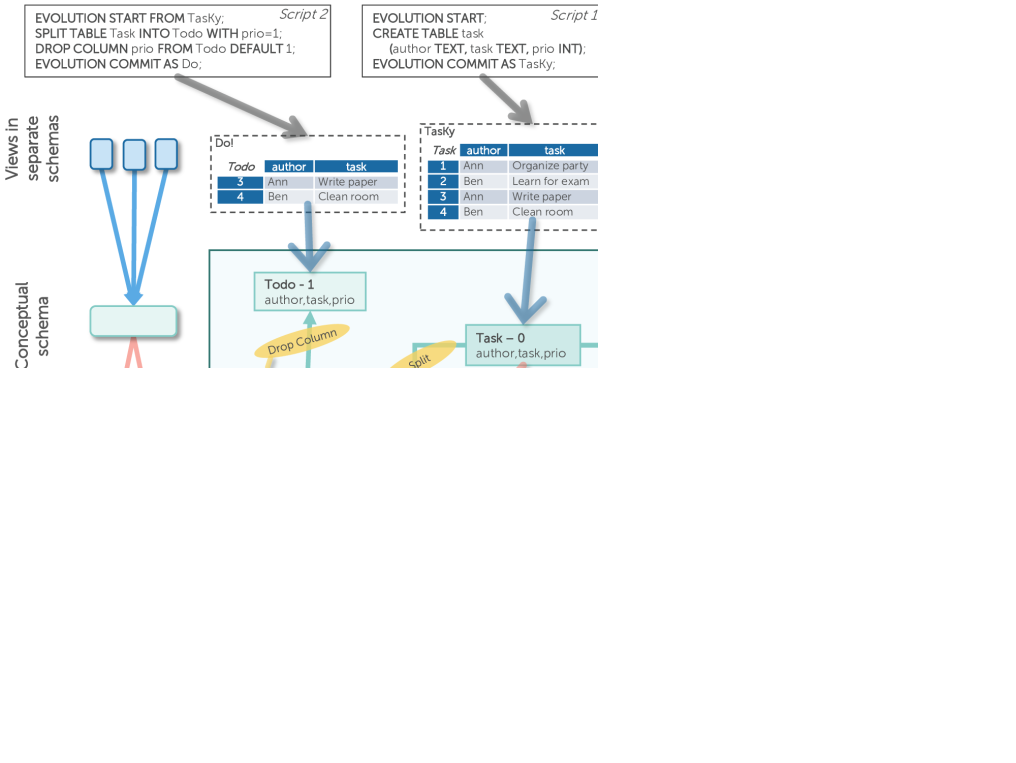
Figure 1: TasKy Example.

In the following, we introduce the co-existing schema version support by InVerDa using the example of a simple task management system called TasKy (cf. Figure 1). TasKy is a desktop application which is backed by a central database. It allows users creating new tasks as well as listing, updating, and deleting them. Each task has an author and a priority. Tasks with priority 1 are the most urgent ones. The first release of TasKy stores all its data in a single table Task(author,task,prio). TasKy has productive go-live and users begin to feed the database with their tasks.

Developer: TasKy gets widely accepted and after some weeks it is extended by a third party phone app called Do! to list most urgent tasks. However Do! expects a different database schema than TasKy is using. The Do! schema consists of a table Todo(author,task) containing only tasks of priority 1. Obviously, the initial schema version needs to stay alive for TasKy, which is broadly installed. InVerDa greatly simplifies the job as it handles all the necessary delta code for the developer. The developer merely executes the BiDEL script for Do! as shown in Figure 1, which instructs InVerDa to derive schema Do! from schema TasKy by splitting a horizontal partition from Task with prio=1 and dropping the priority column. Executing the script creates a new schema including the view Todo as well as delta code for propagating data changes. When a new entry is inserted in Todo, this will automatically insert a corresponding task with priority $1$ to Task in TasKy. Equally, updates and deletions are propagated back to the TasKy schema. Pioneering work like PRIMA allows to create the version Do! as well, however the DEL is not bidirectional, hence write operations are only propagated from TasKy to Do! but not vice versa.

For the next release TasKy2, it is decided to normalize the table Task into Task and Author. For a stepwise roll-out of TasKy2, the old schema of TasKy has to remain alive until all clients have been updated. Again, InVerDa does the job. When executing the BiDEL script as shown in Figure 1, InVerDa creates the schema version TasKy2 and decomposes the table version Task to separate the tasks from their authors while creating a foreign key to maintain the dependency. Additionally, the column author is renamed to name. InVerDa generates delta code to make the TasKy2 schema immediately available. Write operations to any of the three schema versions are propagated to all other versions.

DBA: The initially materialized tables are the targets of create table SMOs. All other table versions are implemented with the help of delta code. The delta code introduces an overhead on read and write accesses to new schema versions. The more SMOs are between schema versions, the more delta code is involved and the higher is the overhead. In our example, the schema versions TasKy2 and Do! have delta code towards the physical table Task. Some weeks after releasing TasKy2 the majority of the users has upgraded to the new version. TasKy2 comes with its own phone app, so the schemas TasKy and Do! are still accessed but merely by a minority of users. It seems appropriate to migrate data physically to the table versions of the TasKy2 schema, now. Traditionally, developers would write a migration script, which moves the data and implements new delta code. All that accumulates to some hundred lines of code, which need to be tested intensively in order to prevent it from messing up our data. With InVerDa, the DBA writes a single line:

MATERIALIZE 'TasKy2';

Upon this statement, InVerDa transparently runs the physical data migration to schema TasKy2, maintaining transaction guarantees, and updates the involved delta code of all schema versions. There is no need to involve any developer. All schema versions stay available; read and write operations are merely propagated to a different set of physical tables, now. Again, these features are facilitated by our bidirectional BiDEL; other approaches either have to materialize all schema versions and provide only forward propagation of data (PRIMA) or have to materialize the latest version and stop serving the old version (PRISM). In sum, InVerDa allows the user to continuously use all schema versions, the developer to continuously develop the applications, and the DBA to independently optimize the physical table schema.

3 INVERDA Architecture

CREATE SCHEMA VERSION $name_{new}$ [FROM $name_{old}$]
CREATE WITH $SMO_{1};\ldots\;SMO_{n};$
DROP SCHEMA VERSION $version_{n};$
CREATE TABLE $R$($c_{1}$,…,$c_{n}$)
DROP TABLE $R$
RENAME TABLE $R$ INTO $R^{\prime}$
RENAME COLUMN $r$ IN $R_{i}$ TO $r^{\prime}$
ADD COLUMN $a$ AS $f$($r_{1}$,…,$r_{n}$) INTO $R_{i}$
DROP COLUMN $r$ FROM $R_{i}$ DEFAULT $f$($r_{1}$,…,$r_{n}$)
DECOMPOSE TABLE $R$ INTO $S$($s_{1},\ldots,s_{n}$)
DECOMPOSE [, $T$($t_{1},\ldots,t_{m}$) ON (PK|FK $fk$|$cond$)]
[OUTER] JOIN TABLE $R$, $S$ INTO $T$ ON (PK|FK $fk$|$cond$)
SPLIT TABLE $T$ INTO $R$ WITH $c_{R}$ [, $S$ WITH $c_{S}$ ]
MERGE TABLE $R$ ($c_{R}$), $S$ ($c_{S}$) INTO $T$

Figure 2: Syntax of BiDEL SMOs.

InVerDa simply builds upon existing relational DBMSes. It adds schema evolution functionality and support for co-existing schema versions. InVerDa functionality is exposed to users via two interfaces: (1) BiDEL (bidirectional database evolution language) and (2) migration commands.

BiDEL provides a comprehensive set of bidirectional SMOs to create a new schema version either from scratch or as an evolution from a given schema version. SMOs evolve source tables to target tables. Each table version is created by one incoming SMO and evolved by arbitrarily many outgoing SMOs. Specifically, BiDEL SMOs allow to create or drop or rename tables and columns, (vertically) decompose or join tables, and (horizontally) split or merge tables (Syntax in Figure 2, general semantics in [7, 9], bidirectional semantics in Section 4). We restrict the considered expressiveness of BiDEL to the relational algebra; the evolution of further artifacts like constraints [5] and functions is promising future work. BiDEL is the youngest child in an evolution of DELs: PRISM [7] is a practically comprehensive DEL that couples schema and data evolution, CoDEL [9] extended PRISM to be relationally complete, and BiDEL extends CoDEL to be bidirectional. As a prerequisite for co-existing schema versions, the unique feature of BiDEL SMOs is bidirectionality. Essentially, the arguments of each BiDEL SMO gather enough information to facilitate full propagation of reads and writes between schema versions in both directions, forward propagation from the old to the new version as well as backward propagation from the new to the old version. For instance, DROP COLUMN requires a function $f(r_{1},\ldots,r_{n})$ that computes the value for the dropped column if a tuple, inserted in the new schema version, is propagated back to an old schema version. Finally, BiDEL allows dropping unnecessary schema versions, which drops the schema version itself but maintains the data if still needed in other versions.

InVerDa’s migration commands allow for changing the physical data representation. By default, data is materialized in the source schema version. Assuming a table is split in a schema evolution step, the data remains physically unsplit. With a migration command the physical data representation of this SMO instance can be changed so that the data is also physically split. Within this work, we focus on non-redundant materialization which means the data is stored either on the source or the target side of the SMO but not on both. Migration commands are very simple. They either materialize a set of table versions or a complete schema version. The latter is merely a convenience command allowing to materialize multiple table versions in one step.

In our prototypical implementation [10], InVerDa creates the co-existing schema versions with views and triggers in a common relational DBMS. InVerDa interacts merely over common DDL and DML statements, data is stored in regular tables, and database applications use the DBMS’s standard query engine. For data accesses of database applications, only the generated views and triggers are used and no InVerDa components are involved. The employed triggers can lead to a cascaded execution, but in a controlled manner as there are no cycles in the version history. Thanks to this architecture, InVerDa easily utilizes existing DBMS components such as physical data storage, indexing, transaction handling, query processing, etc. without reinventing the wheel.

Figure 3: InVerDa integration into DBMS.

Figure 3 outlines the principle components of an InVerDa-equipped DBMS. As can be seen, InVerDa adds three components to the DBMS: (1) the delta code generation creates views and triggers to expose schema versions based on the current physical data representation. Delta code generation is either triggered by a developer issuing BiDEL commands to create a new schema version or by the DBA issuing migration commands to change the physical data representation. The delta code consists of standard commands of the DBMS’s query engine. (2) the migration execution orchestrates the actual migration of data from one physical representation to another and the adaptation of the delta code. The data migration is done with the help of query engine capabilities. (3) the schema version catalog maintains the genealogy of schema versions: It is the history of all schema versions including all table versions as well as the SMO instances and their materialization state. Figure 4 shows the schema version catalog for our TasKy example with the initial materialization.

When developers execute BiDEL scripts, the respective SMO instances and table versions are registered in the schema version catalog. The schema version catalog maintains references to tables in the physical storage that hold the payload data and to auxiliary tables that hold otherwise lost information of the not necessarily information preserving SMOs. The materialization states of the SMOs, which can be changed by the DBA through migration commands, determine which data tables and auxiliary tables are physically present and which are not. InVerDa uses the schema version catalog to generate delta code for new schema versions or for changed physical table schemas. Data accesses of applications are processed by the generated delta code within the DBMS’s query engine. When a developer drops an old schema version that is not used any longer, the schema version is removed from the catalog. However, the respective SMOs are only removed from the catalog in case they are no longer part of an evolution that connects two remaining schema versions.

The schema version catalog is the central knowledge base for all schema versions and the evolution between them. To this end, the catalog stores the genealogy of schema versions by means of a directed acyclic hypergraph $(T,E)$. Each vertex $t\in T$ represents a table version. Each hyperedge $e\in E$ represents one SMO instance, i.e., one table evolution step. An SMO instance $e=(S,T)$ evolves a set of source table versions $S$ into a set of target table versions $T$. Additionally, the schema version catalog stores for every SMO instance the SMO type (split, merge, etc.), the parameter set, and its state of materialization. Each schema version is a subset of all table versions in the system. Schema versions share a table version if the table evolves in-between them. At evolution time, InVerDa uses the catalog to generate delta code that makes all schema versions accessible. At query time, the generated delta code itself is executed by the existing DBMS’s query engine—outside InVerDa components.

Figure 4: Example of schema version catalog.

4 BIDEL - Bidirectional SMOs

BiDEL’s unique feature is the bidirectional semantics of its SMOs, which is the basis for InVerDa’s co-existing schema versions. We highlight the design principles behind BiDEL SMOs and formally validate their bidirectionality. All BiDEL SMOs follow the same design principles. Without loss of generality, the SPLIT SMO is used as a representative example in this section to explain the concepts. The remaining SMOs are introduced in Appendix B.

Figure 5 illustrates the principle structure of a single SMO instance resulting from the sample statement

SPLIT TABLE $T$ INTO $R$ WITH $c_{R}$, $S$ WITH $c_{S}$

which horizontally splits a source table $T$ into two target tables $R$ and $S$ based on conditions $c_{R}$ and $c_{S}$. Assuming both schemas are materialized, reads and writes on both schema versions can simply be delegated to the corresponding data tables $T_{D}$, $R_{D}$, and $S_{D}$, respectively. However, InVerDa materializes data non-redundantly on one side of the SMO instance, only. If the data is physically stored on the source side of an SMO instance, the SMO instance is called virtualized; with data stored on the target side it is called materialized. In any case, reads and writes on the unmaterialized side are mapped to the materialized side.

The semantics of each SMO is defined by two functions $\gamma_{tgt}$ and $\gamma_{src}$ which describe precisely the mapping from the source side to the target side and vice versa, respectively. Assuming the target side of SPLIT is materialized, all reads on $T$ are mapped by $\gamma_{src}$ to reads on $R_{D}$ and $S_{D}$; and writes on $T$ are mapped by $\gamma_{tgt}$ to writes on $R_{D}$ and $S_{D}$. While the payload data of $R$, $S$, and $T$ is stored in the physical tables $R_{D}$, $S_{D}$, and $T_{D}$, the tables $R^{-}$, $S^{+}$, $S^{-}$, $R^{*}$, $S^{*}$, and $T^{\prime}$ are auxiliary tables for the SPLIT SMO to prevent information loss. Note that the semantics of SMOs is complete, if reads and writes on both source and target schema work correctly regardless on which of both sides the data is physically stored. This basically means that each schema version acts like a full-fledged database schema; however it does not enforce that data written in any version is also fully readable in other versions. In fact, BiDEL ensures this for all SMOs except of those that create redundancy—in these cases the developer specifies a preferred replica beforehand.

Obviously, there are different ways of defining $\gamma_{tgt}$ and $\gamma_{src}$; in this paper, we propose one way that systematically covers all potential inconsistencies and is bidirectional. We aim at a non-redundant materialization, which also includes that the auxiliary tables merely store the minimal set of required auxiliary information. Starting from the basic semantics of the SMO—e.g. the splitting of a table—we incrementally detect inconsistencies that contradict the bidirectional semantics and introduce respective auxiliary tables. The proposed rule sets can serve as a blueprint, since they clearly outline which information needs to be stored to achieve bidirectionality.

To define $\gamma_{tgt}$ and $\gamma_{src}$, we use Datalog—a compact and solid formalism that facilitates both a formal evaluation of bidirectionality and easy delta code generation. Precisely, we use Datalog rule templates instantiated with the parameters of an SMO instance. For brevity of presentation, we use some extensions to the standard Datalog syntax: For variables, small letters represent single attributes and capital letters lists of attributes. For equality predicates on attribute lists, both lists need to have the same length and same content, i.e. for $A=(a_{1},\ldots,a_{n})$ and $B=(b_{1},\ldots,b_{m})$, $A=B$ holds if $n=m\wedge a_{1}=b_{1}\wedge\ldots\wedge a_{n}=b_{n}$. All tables have an attribute $p$, an InVerDa-managed identifier to uniquely identify tuples across versions. Additionally, $p$ ensures that the multiset semantics of a relational database fits with the set semantics of Datalog, as the unique key $p$ prevents equal tuples in one relation. For a table $T$ we assume $T(p,\_)$ and $\neg T(p,\_)$ to be safe predicates since any table can be projected to its key.

For the exemplary SPLIT, let’s assume this SMO instance is materialized, i.e. data is stored on the target side, and let’s consider the $\gamma_{tgt}$ mapping function first. SPLIT horizontally splits a table $T$ from the source schema into two tables $R$ and $S$ in the target schema based on conditions $c_{R}$ and $c_{S}$:

$$R(p,A) \leftarrow T(p,A),c_{R}(A)$$ (1)

$$S(p,A) \leftarrow T(p,A),c_{S}(A)$$ (2)

The conditions $c_{R}$ and $c_{S}$ can be arbitrarily set by the user so that Rule 1 and Rule 2 are insufficient wrt. the desired bidirectional semantics, since the source table $T$ may contain tuples neither captured by $c_{R}$ nor by $c_{S}$. In order to avoid inconsistencies and make the SMO bidirectional, such tuples are stored on the target side in the auxiliary table $T^{\prime}$:

$$T^{\prime}(p,A) \leftarrow T(p,A),\neg c_{R}(A),\neg c_{S}(A)$$ (3)

Figure 5: Mapping functions of single SPLIT SMO.

Let’s now consider the $\gamma_{src}$ mapping function for reconstructing $T$ while the target side is still considered to be materialized. Reconstructing $T$ from the target side is essentially a union of $R$, $S$, and $T^{\prime}$. Nevertheless, $c_{R}$ and $c_{S}$ are not necessarily disjoint. One source tuple may occur as two equal but independent instances in $R$ and $S$. We call such two instances twins. Twins can be updated independently resulting in separated twins, i.e. two tuples—one in $R$ and one in $S$—with equal key $p$ but different value for the other attributes. To resolve this ambiguity and make the SMO bidirectional, we consider the first twin in $R$ to be the primus inter pares and define $\gamma_{src}$ of SPLIT to propagate back all tuples in $R$ as well as those tuples in $S$ not contained in $R$:

$$T(p,A) \leftarrow R(p,A)$$ (4)

$$T(p,A) \leftarrow S(p,A),\neg R(p,\_)$$ (5)

$$T(p,A) \leftarrow T^{\prime}(p,A)$$ (6)

The Rules 1–6 define sufficient semantics for SPLIT as long as the target side is materialized.

Let’s now assume the SMO instance is virtualized, i.e. data is stored on the source side, and let’s keep considering the $\gamma_{src}$ mapping function. Again, $R$ and $S$ can contain separated twins—unequal tuples with equal key $p$. According to Rule 5, $T$ stores only the separated twin from $R$. To avoid losing the other twin in $S$, it is stored in the auxiliary table $S^{+}$:

$$S^{+}(p,A) \leftarrow S(p,A),R(p,A^{\prime}),A\neq A^{\prime}$$ (7)

Accordingly, $\gamma_{tgt}$ has to reconstruct the separated twin in $S$ from $S^{+}$ instead of $T$ (concerns Rule 2). Twins can also be deleted independently resulting in a lost twin. Given the data is materialized on the source side, a lost twin would be directly recreated from its other twin via $T$. To avoid this information gain and keep lost twins lost, $\gamma_{src}$ keeps the keys of lost twins from $R$ and $S$ in auxiliary tables $R^{-}$ and $S^{-}$:

$$R^{-}(p) \leftarrow S(p,A),\neg R(p,\_),c_{R}(A)$$ (8)

$$S^{-}(p) \leftarrow R(p,A),\neg S(p,\_),c_{S}(A)$$ (9)

Accordingly, $\gamma_{tgt}$ has to exclude lost twins stored in $R^{-}$ from $R$ (concerns Rule 1) and those in $S^{-}$ from $S$ (concerns Rule 2). Twins result from data changes issued to the target schema containing $R$ and $S$ which can also lead to tuples that do not meet the conditions $c_{R}$ resp. $c_{S}$. In order to ensure that the reconstruction of such tuples is possible from a materialized table $T$, auxiliary tables $R^{*}$ and $S^{*}$ are employed for identifying those tuples using their identifiers (concerns Rules 1 and 2).

$$S^{*}(p) \leftarrow S(p,A),\neg c_{S}(A)$$ (10)

$$R^{*}(p) \leftarrow R(p,A),\neg c_{R}(A)$$ (11)

The full rule sets of $\gamma_{tgt}$ respectively $\gamma_{src}$ are now bidirectional and defined as follows:

$$\mathbf{\gamma_{tgt}:}$$

$$R(p,A) \leftarrow T(p,A),c_{R}(A),\neg R^{-}(p)$$ (12)

$$R(p,A) \leftarrow T(p,A),R^{*}(p)$$ (13)

$$S(p,A) \leftarrow T(p,A),c_{S}(A),\neg S^{-}(p),\neg S^{+}(p,\_)$$ (14)

$$S(p,A) \leftarrow S^{+}(p,A)$$ (15)

$$S(p,A) \leftarrow T(p,A),S^{*}(p),\neg S^{+}(p,\_)$$ (16)

$$T^{\prime}(p,A) \leftarrow T(p,A),\neg c_{R}(A),\neg c_{S}(A),\neg R^{*}(p),\neg S^{*}(p)$$ (17)

$$\mathbf{\gamma_{src}:}$$

$$T(p,A) \leftarrow R(p,A)$$ (18)

$$T(p,A) \leftarrow S(p,A),\neg R(p,\_)$$ (19)

$$T(p,A) \leftarrow T^{\prime}(p,A)$$ (20)

$$R^{-}(p) \leftarrow S(p,A),\neg R(p,\_),c_{R}(A)$$ (21)

$$R^{*}(p) \leftarrow R(p,A),\neg c_{R}(A)$$ (22)

$$S^{+}(p,A) \leftarrow S(p,A),R(p,A^{\prime}),A\neq A^{\prime}$$ (23)

$$S^{-}(p) \leftarrow R(p,A),\neg S(p,\_),c_{S}(A)$$ (24)

$$S^{*}(p) \leftarrow S(p,A),\neg c_{S}(A)$$ (25)

The semantics of all other BiDEL SMOs are defined in a similar way, see Appendix B. This precise definition of BiDEL’s SMOs, is the basis for the formal validation of their bidirectionality.

5 Formal evaluation of BIDEL’s 
bidirectionality

BiDEL’s SMOs are bidirectional, because, no matter whether the data is (1) materialized on the source side (SMO is virtualized) or (2) materialized on the target side (SMO is materialized), both sides behave like a full-fledged single-schema database. To formally evaluate this claim, we consider the two cases (1) and (2) independently. Let’s start with case (1); the data is materialized on the source side. For a correct target-side propagation, the data $D_{tgt}$ at the target side has to be mapped by $\gamma_{src}$ to the data tables and auxiliary tables at the source side (write) and mapped back by $\gamma_{tgt}$ to the data tables on the target side (read) without any loss or gain visible in the data tables at the target side. Similar conditions have already been defined for symmetric relational lenses [11]—given data at the target side, storing it at the source side, and mapping it back to target should return the identical data at the target side. For the second case (2) it is vice versa. Formally, an SMO has bidirectional semantics if the following holds:

$$D_{tgt} =\gamma_{tgt}^{data}(\gamma_{src}(D_{tgt}))$$ (26)

$$D_{src} =\gamma_{src}^{data}(\gamma_{tgt}(D_{src}))$$ (27)

Data tables that are visible to the user need to match these bidirectionality conditions. As indicated by the index $\gamma^{data}$, we project away potentially created auxiliary tables; however, they are always empty except for SMOs that calculate new values: e.g. adding a column requires to store the calculated values when data is stored at the source side to ensure repeatable reads. The bidirectionality conditions are shown by applying and simplifying the Datalog rule sets that define the mappings $\gamma_{src}$ and $\gamma_{tgt}$. We label the original relations to distinguish them from the resulting relation, apply $\gamma_{src}$ and $\gamma_{tgt}$ in the order according to Condition 26 or 27, and compare the outcome to the original relation. It has to be identical. As neither the rules for a single SMO nor the version genealogy have cycles, there is no recursion at all, which simplifies evaluating the combined Datalog rules.

In the following, we introduce some basic notion about Datalog rules as basis for the formal evaluation. A Datalog rule is a clause of the form $H\leftarrow L_{1},\ldots,L_{n}$ with $n\geq 1$ where $H$ is an atom denoting the rule’s head, and $L_{1},\ldots,L_{n}$ are literals, i.e. positive or negative atoms, representing its body. For a given rule $r$, we use $\texttt{head}(r)$ to denote its head $H$ and $\texttt{body}(r)$ to denote its set of body literals $L_{1},\ldots,L_{n}$. In the mapping rules defining $\gamma_{src}$ and $\gamma_{tgt}$, every $\texttt{head}(r)$ is of the form $q^{r}(p,Y)$ where $q^{r}$ is the derived predicate, $p$ is the InVerDa-managed identifier, and $Y$ is a potentially empty list of variables. Further, we use $\texttt{pred}(r)$ to refer to the predicate symbol of $\texttt{head}(r)$. For a set of rules $\mathcal{R}$, $\mathcal{R}^{q}$ is defined as $\left\{r\mid r\in\mathcal{R}\wedge\texttt{pred}(r)=q\right\}$. For a body literal $L$, we use $\texttt{pred}(L)$ to refer to the predicate symbol of $L$ and $\texttt{vars}(L)$ to denote the set of variables occurring in $L$. In the mapping rules, every literal $L\in\texttt{body}(r)$ is of the form either $q^{r}_{i}(p,Y^{r}_{i},X^{r}_{i})$ or $c^{r}(Y^{r}_{i},X^{r}_{i})$, where $Y^{r}_{i}\subset Y$ are the variables occurring in $L$ and $\texttt{head}(r)$ and $X^{r}_{i}$ are the variables occurring in $L$ but not in $\texttt{head}(r)$. Generally, we use capital letters to denote multiple variables. For a set of literals $\mathcal{K}$, $\texttt{vars}(\mathcal{K})$ denotes $\bigcup_{L\in\mathcal{K}}\texttt{vars}(L)$. The following lemmas are used for simplifying a given rule set $\mathcal{R}$ into a rule set $\mathcal{R^{\prime}}$ such that $\mathcal{R^{\prime}}$ derives the same facts as $\mathcal{R}$.

Lemma 1 (Deduction)

Let $L\equiv q^{r}(p,Y)$ be a literal in the body of a rule $r$. For a rule $s\in\mathcal{R}^{\texttt{pred}(L)}$ let $\texttt{rn}(s,L)$ be rule $s$ with all variables occurring in the head of $s$ at positions of $Y$ variables in $L$ be renamed to match the corresponding $Y$ variable and all other variables be renamed to anything not in $\texttt{vars}(\texttt{body}(r))$. If $L$ is

1. a positive literal, $s$ can be applied to $r$ to get rule set $r(s)$ of the form $\left\{\texttt{head}(r)\leftarrow\texttt{body}(r)\setminus\left\{L\right\}\cup\texttt{body}(\texttt{rn}(s,L))\right\}$.

2. a negative literal, $s$ can be applied to $r$ to get rule set $r(s)=$ $\left\{\texttt{head}(r)\leftarrow\texttt{body}(r)\setminus\left\{L\right\}\cup t(K)\mid K\in\texttt{body}(\texttt{rn}(s,L)))\right\}$
   with either $t(K)=\left\{\neg q^{s}_{i}(p,Y^{s}_{i},\_)\right\}$ if $K\equiv q^{s}_{i}(p,Y^{s}_{i},X^{s}_{i})$ or $t(K)=\{q^{s}_{j}(p,Y^{s}_{j},X^{s}_{j})\mid q^{s}_{j}(p,Y^{s}_{i},X^{s}_{j})\in\texttt{body}(\texttt{rn}(s,L))\wedge X^{s}_{j}\cap X^{s}_{i}\neq\emptyset\}\cup\left\{c^{r}(Y^{s}_{i},X^{s}_{i})\right\}$ if $K\equiv c^{r}(Y^{s}_{i},X^{s}_{i})$.

For a given $p$, let $r$ be every rule in $\mathcal{R}$ having a literal $L\equiv p(X,Y)$ in its body. Accordingly, $\mathcal{R}$ can be simplified by replacing all rules $r$ and all $s\in\mathcal{R}^{p}$ with all $r(s)$ applications to $\mathcal{R}\setminus(\left\{r\right\}\cup\mathcal{R}^{p})\cup(\bigcup_{s\in\mathcal{R}^{\texttt{pred}(L)}}r(s))$.

Lemma 2 (Empty Predicate)

Let $r\in\mathcal{R}$ be a rule, $L$ be a literal in the body $L\in\texttt{body}(r)$ and the relation $\texttt{pred}(L)$ is known to be empty. If $L$ is a positive literal, $r$ can be removed from $\mathcal{R}$. If $L$ is a negative literal, $r$ can be simplified to $\texttt{head}(r)\leftarrow\texttt{body}(r)\setminus\left\{L\right\}$.

Lemma 3 (Tautology)

Let $r,s\in\mathcal{R}$ be rules and $L$ and $K$ be literals in the bodies of $r$ and $s$, respectively, where $r$ and $s$ are identical except for $L$ and $K$, i.e. $\texttt{head}(r)=\texttt{head}(s)$ and $\texttt{body}(r)\setminus\left\{L\right\}=\texttt{body}(s)\setminus\left\{K\right\}$, or can be renamed to be so. If $K\equiv\neg L$, $r$ can be simplified to $\texttt{head}(r)\leftarrow\texttt{body}(r)\setminus\left\{L\right\}$ and $s$ can be removed from $\mathcal{R}$.

Lemma 4 (Contradiction)

Let $r\in\mathcal{R}$ be a rule and $L$ and $K$ be literals in its body $L,K\in\texttt{body}(r)$. If $K\equiv\neg L$, $r$ can be removed from $\mathcal{R}$.

Lemma 5 (Unique Key)

Let $r\in\mathcal{R}$ be a rule and $q(p,X)$ and $q(p,Y)$ be literals in its body. Since, by definition, $p$ is a unique identifier, $r$ can be modified to $\texttt{head}(r)\leftarrow\texttt{body}(r)\cup\left\{X=Y\right\}$.

In this paper, we use these lemmas to show bidirectionality for the materialized SPLIT SMO in detail. Hence, Equation 27 needs to be satisfied. Writing data $T_{D}$ from source to target-side results in the mapping $\gamma_{tgt}(T_{D})$. With target-side materialization all source-side auxiliary tables are empty. Thus, $\gamma_{tgt}(T_{D})$ can be simplified with Lemma 2:

$$R(p,A) \leftarrow T_{D}(p,A),c_{R}(A)$$ (28)

$$S(p,A) \leftarrow T_{D}(p,A),c_{S}(A)$$ (29)

$$T^{\prime}(p,A) \leftarrow T_{D}(p,A),\neg c_{R}(A),\neg c_{S}(A)$$ (30)

Reading the source-side data back from $R$, $S$, and $T^{\prime}$ to $T$ adds the rule set $\gamma_{src}$ (Rule 18–25) to the mapping. Using Lemma 1, the mapping $\gamma_{src}(\gamma_{tgt}(T_{D}))$ simplifies to:

$$T(p,A)\leftarrow T_{D}(p,A),c_{R}(A)$$ (31)

$$T(p,A)\leftarrow T_{D}(p,A),c_{S}(A),\neg T_{D}(p,A)$$ (32)

$$T(p,A)\leftarrow T_{D}(p,A),c_{S}(A),\neg c_{R}(A)$$ (33)

$$T(p,A)\leftarrow T_{D}(p,A),\neg c_{S}(A),\neg c_{R}(A)$$ (34)

$$R^{-}(p)\leftarrow T_{D}(p,A),c_{S}(A),\neg T_{D}(p,A),c_{R}(A)$$ (35)

$$R^{-}(p)\leftarrow T_{D}(p,A),c_{S}(A),\neg c_{R}(A),c_{R}(A)$$ (36)

$$R^{*}(p)\leftarrow T_{D}(p,A),c_{R}(A),\neg c_{R}(A)$$ (37)

$$S^{+}(p,A)\leftarrow T_{D}(p,A),c_{S}(A),T_{D}(p,A^{\prime}),c_{R}(A^{\prime}),A\!\neq\!A^{\prime}$$ (38)

$$S^{-}(p)\leftarrow T_{D}(p,A),c_{R}(A),\neg T_{D}(p,A),c_{S}(A)$$ (39)

$$S^{-}(p)\leftarrow T_{D}(p,A),c_{R}(A),\neg c_{S}(A),c_{S}(A)$$ (40)

$$S^{*}(p)\leftarrow T_{D}(p,A),c_{S}(A),\neg c_{S}(A)$$ (41)

With Lemma 4, we omit Rule 32 as it contains a contradiction. With Lemma 3, we reduce Rules 33 and 34 to Rule 43 by removing the literal $c_{S}(A)$. The resulting rules for $T$

$$T(p,A) \leftarrow T_{D}(p,A),c_{R}(A)$$ (42)

$$T(p,A) \leftarrow T_{D}(p,A),\neg c_{R}(A)$$ (43)

can be simplified again with Lemma 3 to

$$T(p,A) \leftarrow T_{D}(p,A)\quad.$$ (44)

For Rule 38, Lemma 5 implies $A=A^{\prime}$, so this rule can be removed based on Lemma 4. Likewise, the Rules 36–41 have contradicting literals on $T_{D}$, $c_{R}$, and $c_{S}$ respectively so that Lemma 4 applies here as well. The result clearly shows that data $T_{D}$ in $D_{src}$ is mapped by $\gamma_{src}(\gamma_{tgt}(D_{src}))$ to the target side and back to $D_{src}$ without any information loss or gain:

$$\mathbf{\gamma_{src}(\gamma_{tgt}(D_{src})):}\;\; T(p,A)\leftarrow T_{D}(p,A)\qed$$ (45)

So, $D_{src}=\gamma_{src}(\gamma_{tgt}(D_{src}))$ holds. Remember that the auxiliary tables only exist on the materialized side of the SMO (target in this case). Hence, it is correct that there are no rules left producing data for the source-side auxiliary. The same can be done for Equation 26 as well (Appendix A). As expected, the simplification of $\gamma_{tgt}(\gamma_{src}(D_{tgt}))$ results in

$$\mathbf{\gamma_{tgt}(\gamma_{src}(D_{tgt})):}\;\; R(p,A)\leftarrow R_{D}(p,A)$$ (46)

$$S(p,A)\leftarrow S_{D}(p,A)$$ (47)

This formal evaluation works for the remaining BiDEL SMOs, as well (Appendix B). BiDEL’s SMOs ensure that given data at any schema version $V_{n}$ that is propagated and stored at a direct predecessor $V_{n-1}$ or direct successor schema version $V_{n+1}$ can always be read completely and correctly in $V_{n}$. To our best knowledge, we are the first to design a set of powerful SMOs and validate their bidirectionality according to the criteria of symmetric relational lenses.

Write operations: Bidirectionality also holds after write operations: When updating a not-materialized schema version, this update is propagated to the materialized schema in a way that it is correctly reflected when reading the updated data again. Given a materialized SMO, we apply a write operation $\Delta_{src}(D_{src})$ to given data on the source side. $\Delta_{src}(D_{src})$ can both insert and update and delete data. Initially, we store $D_{src}$ at the target side using $D_{tgt}=\gamma_{tgt}(D_{src})$. To write at the source side, we have to temporarily map back the data to the source with $\gamma_{src}^{data}(D_{tgt})$, apply the write $\Delta_{src}$, and map the updated data back to target with $D_{tgt}^{\prime}=\gamma_{tgt}(\Delta_{src}(\gamma_{src}^{data}(D_{tgt})))$. Reading the data from the updated target $\gamma_{src}^{data}(D_{tgt}^{\prime})$ has to be equal to applying the write operation $\Delta_{src}(D_{src})$ directly on the source side.

$$\Delta_{src}(D_{src}) =\gamma_{src}^{data}(\gamma_{tgt}(\Delta_{src}(\gamma_{src}^{data}(\gamma_{tgt}(D_{src})))))$$ (48)

We have already shown that $D=\gamma_{src}^{data}(\gamma_{tgt}(D))$ holds for any data $D$ at the target side, so that Equation 48 reduces to $\Delta_{src}(D_{src})=\Delta_{src}(D_{src})$. Hence writes are correctly propagated through the SMOs. The same holds vice versa for writing at the target-side of virtualized SMOs:

$$\Delta_{tgt}(D_{tgt}) =\gamma_{tgt}^{data}(\gamma_{src}(\Delta_{tgt}(\gamma_{tgt}^{data}(\gamma_{src}(D_{tgt})))))$$ (49)

Chains of SMOs: Further, the bidirectionality of BiDEL SMOs also holds for chains of SMOs: $smo_{1},\ldots smo_{n}$, where $\gamma_{i,src/tgt}$ is the respective mapping of $smo_{i}$. Analogous to symmetric relational lenses [11], there are no side-effects between multiple BiDEL SMOs. So, BiDEL’s bidirectionality is also guaranteed along chains of SMOs:

$$D_{tgt} =\gamma_{n,tgt}^{data}(\ldots\gamma_{1,tgt}(\gamma_{1,src}(\ldots\gamma_{n,src}(D_{tgt}))))$$ (50)

$$D_{src} =\gamma_{1,src}^{data}(\ldots\gamma_{n,src}(\gamma_{n,tgt}(\ldots\gamma_{1,tgt}(D_{src}))))$$ (51)

This bidirectionality ensures logical data independence, since any schema version can now be read and written without information loss or gain, no matter where the data is actually stored. The auxiliary tables keep the otherwise lost information and we have formally validated their feasibility. With the formal guarantee of bidirectionality—also along chains of SMOs and for write operations—we have laid a solid formal foundation for InVerDa’s delta code generation.

6 Delta Code Generation

Figure 6: Three different cases in delta code generation.

To make a schema version available, InVerDa translates the $\gamma_{src}$ and $\gamma_{tgt}$ mapping functions into delta code—specifically views and triggers. Views implement delta code for reading; triggers implement delta code for writing. In a schema versions genealogy, a single table version is the target of one SMO instance and the source for a number of SMO instances. The delta code for a specific table version depends on the materialization state of the table’s adjacent SMOs.

To determine the right rule sets for delta code generation, consider the schema genealogy in Figure 6. Table version $T_{i}$ is materialized, hence the two subsequent SMO instances, $i-1$ and $i$ store their data at the target side (materialized), while the two subsequent SMO instances, $i+1$ and $i+2$ are set to source-side materialization (virtualized). Without loss of generality, three cases for delta code generation can be distinguished, depending on the direction a specific table version needs to go for to reach the materialized data.

Case 1 – local:

The incoming SMO is materialized and all outgoing SMOs are virtualized. The data of $T_{i}$ is stored in the data table $D_{i}$ and is directly accessible.

Case 2 – forwards:

The incoming SMO and one outgoing SMO are materialized. The data of $T_{i-1}$ is stored in newer versions along the schema genealogy, so data access is propagated with $\gamma_{src}$ (read) and $\gamma_{tgt}$ (write) of $\texttt{\footnotesize{SMO}}_{i}$.

Case 3 – backwards:

The incoming SMO and all outgoing SMOs are virtualized. The data of $T_{i+1}$ is stored in older versions along the schema genealogy, so data access is propagated with $\gamma_{tgt}$ (read) and $\gamma_{src}$ (write) of $\texttt{\footnotesize{SMO}}_{i+1}$.

In Case 1, delta code generation is trivial. In Case 2 and  3, InVerDa essentially translates the Datalog rules defining the relevant mapping functions into view and trigger definitions. Figure 7 illustrates the general pattern of the translation of Datalog rules to a view definition. As a single table can be derived by multiple rules, e.g. Rule 18–20, a view is a union of subqueries each representing one of the rules. For each subquery, InVerDa lists all attributes of the rule head in the select clause. Within a nested subselect these attributes are either projected from the respective table version or derived by a function. All positive literals referring to other table versions or auxiliary tables are listed in the from clause. Further, InVerDa adds for all attributes occurring in multiple positive literals respective join conditions to the where clause. Finally, conditions, such as $c_{S}(X)$, and negative literals, which InVerDa adds as a NOT EXISTS(<subselect for the literal>) condition, complete the where-clause.

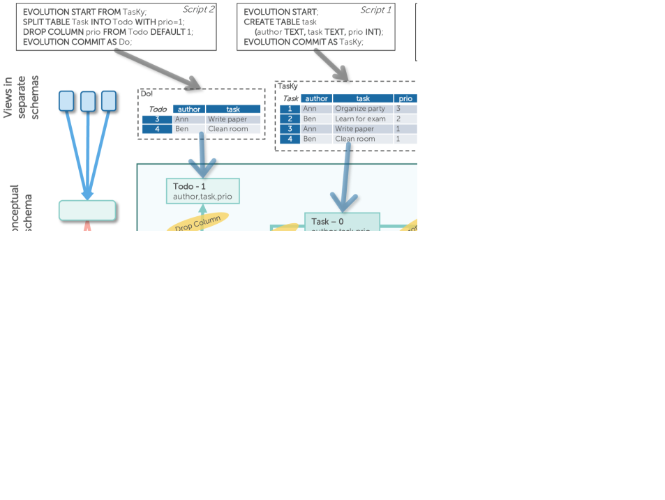
Figure 7: SQL generation from Datalog rules.

For writing, InVerDa generates three triggers on each table version: for inserts, deletes, and updates. To not recompute all data of the materialized side after each write operation at the not-materialized side of an SMO, InVerDa adopts an update propagation technique for Datalog rules [2] that results in minimal write operations. For instance, an insert operation $\Delta_{T}^{+}(p,A)$ on the table version $T$ propagated back to the source side of a materialized SPLIT SMO results in the following update rules:

$$\Delta^{+}_{R}(p,A)\leftarrow\Delta^{+}_{T}(p,A), \mathtt{new}\;c_{R}(A),\mathtt{old}\;\neg R(p,A)$$ (52)

$$\Delta^{+}_{S}(p,A)\leftarrow\Delta^{+}_{T}(p,A), \mathtt{new}\;c_{S}(A),\mathtt{old}\;\neg S(p,A)$$ (53)

$$\Delta^{+}_{T^{\prime}}(p,A)\leftarrow\Delta^{+}_{T}(p,A), \mathtt{new}\;\neg c_{R}(A),\neg c_{S}(A),\mathtt{old}\;\neg T^{\prime}(p,A)$$ (54)

The propagation can handle multiple write operations at the same time and distinguishes between old and new data, which represents the state before and after applying other write operations. The derived update rules match the intuitive expectations: The inserted tuple is propagated to $R$ or to $S$ or to $T^{\prime}$ given it satisfies either $c_{R}$ or $c_{S}$ or none of them. The additional conditions on the $\mathtt{old}$ literals ensure minimality by checking whether the tuple already exists. To generate trigger code from the update rule, InVerDa applies essentially the same algorithm as for view generation.

Writes performed by a trigger on a table version further trigger the propagation along the schema genealogy to the other table versions as long as the respective update rules deduce write operations, i.e. as long as some data is physically stored with a table version either in the data table or in auxiliary tables. With the generated delta code, InVerDa propagates writes on any schema version to every other co-existing schema version in a schema genealogy.

7 Migration Procedure

The materialization states of all SMO instances in a schema genealogy form the materialization schema. The materialization schema determines the physical table schema, i.e. which table versions are directly stored in physical storage. For the TasKy example—Figure 1—this entails five different possible materialization schemas $M$, each implying a different physical table schema $P$ as shown in Table 2.

$M$	$P$
$\emptyset$	$\left\{\texttt{\footnotesize{Task-0}}\right\}$
$\left\{\texttt{\footnotesize{SPLIT}}\right\}$	$\left\{\texttt{\footnotesize{Task-0}}\right\}$
$\left\{\texttt{\footnotesize{SPLIT}},\texttt{\footnotesize{DROP COLUMN}}\right\}$	$\left\{\texttt{\footnotesize{Todo-1}}\right\}$
$\left\{\texttt{\footnotesize{DECOMPOSE}}\right\}$	$\left\{\texttt{\footnotesize{Task-1}},\texttt{\footnotesize{Author-0}}\right\}$
$\left\{\texttt{\footnotesize{DECOMPOSE}},\texttt{\footnotesize{RENAME}}\right\}$	$\left\{\texttt{\footnotesize{Task-1}},\texttt{\footnotesize{Author-1}}\right\}$

Table 2: Possible materialization schemas and the corresponding physical table schema in the TasKy example.

The materialization schema has huge impact on the performance of a given workload. Workload changes such as increased usage of newer schema versions demand adaptations of the materialization schema. InVerDa facilitates such an adaptation with a foolproof migration command. The migration command allows moving data non-redundantly along the schema genealogy to those table versions where the given workload causes the least overhead for propagating reads and writes. Initially, all SMOs except of the create table SMOs are virtualized, i.e. only initially created table versions are in the physical table schema. A new materialization schema is derived from a given valid materialization schema by changing the materialization state of selected SMO instances. Formally, two conditions must hold for a materialization schema to be valid. For an SMO $s$, we denote the source table versions as $\texttt{src}(s)$. For each table version $t$ we denote the incoming SMO with $\texttt{in}(t)$ and the set of outgoing SMOs with $\texttt{out}(t)$. A materialization is valid iff:

$$\forall s\!\in\!M\ \forall t\!\in\!\texttt{src}(s)\ \left(\texttt{in}(t)\in M\right)$$ (55)

$$\forall s\!\in\!M\ \forall t\!\in\!\texttt{src}(s)\ \nexists o\!\in\!\left(\texttt{out}(t)\!\setminus\!\left\{s\right\}\right)\ \left(o\in M\right)$$ (56)

The first condition ensures that all source table versions are in the materialization schema. The second condition ensures that no source table version is already taken by another materialized SMO.

In the migration command, the DBA lists the table versions that should be materialized. For instance:

MATERIALIZE 'TasKy2.task', 'TasKy2.author';

InVerDa determines with the schema version catalog the corresponding materialization schema and checks, whether it is valid according to the conditions above. If valid, InVerDa automatically creates the new physical tables including auxiliary tables in the physical storage, migrates the data, regenerates all necessary delta code, and deletes all old physical tables. The actual data migration relies on the same SQL generation routines as used for view generation. From a user perspective, all schema versions still behave the same after a migration. However, any data access is now propagated to the new physical table schema resulting in a better performance for schema versions that are evolution-wise close to this new physical schema. This migration is triggered by one single line of code, so adaptation to the current workload becomes a comfortable thing to do for database administrators.

8 Evaluation

InVerDa brings huge advantages for software systems by decoupling the different goals of different stakeholders. Users can continuously access all schema versions, while developers can focus on the actual continuous implementation of the software without caring about former versions. Above all, the DBA can change the physical table schema of the database to optimize the overall performance without restricting the availability of the co-existing schema versions or invalidating the developers’ code. In Section 8.1, we show how InVerDa reduces the length and complexity of the code to be written by the developer and thereby yields more robust and maintainable solutions. InVerDa automatically generates the delta code based on the discussed Datalog rules. In Section 8.2, we measure the overhead of accessing data through InVerDa’s delta code compared to a handwritten SQL implementation of co-existing schema versions and show that it is reasonable. In Section 8.3, we show that the possibility to easily adapt the physical table schema to a changed workload outweighs the small overhead of InVerDa’s automatically generated delta code. Materializing the data according to the most accessed version speeds up the data access significantly.

InVerDa	Initially	Evolution	Migration
Lines of Code	1	3	1
Statements	1	3	1
Characters	54	152	19
SQL (Ratio)	Initially	Evolution	Migration
Lines of Code	1 ($\times$1.00)	359 ($\times$119.67)	182 ($\times$182.00)
Statements	1 ($\times$1.00)	148 ($\times$49.33)	79 ($\times$79.00)
Characters	54 ($\times$1.00)	9477 ($\times$62.35)	4229 ($\times$222.58)

Table 3: Ratio between SQL and InVerDa delta code.

Setup: For the measurements, we use three different data sets to gather a holistic idea of InVerDa’s characteristics. We use (1) our TasKy example as a middle-sized and comprehensive scenario, (2) $171$ schema versions of Wikimedia [7] as a long real-world scenario, and (3) short synthetic scenarios for all possible combinations of two SMOs. We measure single thread performance of a PostgreSQL 9.4 database with co-existing schema versions on a Core i7 machine with 2,4GHz and 8GB memory.

8.1 Simplicity and Robustness

Most importantly, we show that InVerDa unburdens developers by rendering the expensive and error-prone task of manually writing delta code unnecessary. We show this using both the TasKy example and Wikimedia.

TasKy: We implement the evolution from TasKy to TasKy2 with handwritten and hand-optimized SQL and compare this code to the equivalent BiDEL statements. We manually implemented (1) creating the initial TasKy schema, (2) creating the additional schema version TasKy2 with the respective views and triggers, and (3) migrating the physical table schema to TasKy2 and adapting all existing delta code. This handwritten SQL code is much longer and much more complex than achieving the same goal with BiDEL. Table 3 shows the lines of code (LOC) required with SQL and BiDEL, respectively, as well as the ratio between these values. As there is no general coding style for SQL, LOC is a rather vague measure. We also include the number of statements and the number of characters (consecutive white-space characters counted as one) as more objective measures to get a clear picture. Obviously, creating the initial schema is equally complex for both approaches. However, evolving to the new schema version TasKy2 and migrating the data accordingly requires $359$ and $182$ lines of SQL code respectively, while we can express the same with $3$ and $1$ lines with BiDEL. Moreover, the SQL code is also more complex, as indicated by the average number of character per statement. While BiDEL is working exclusively on the visible schema versions, with handwritten SQL developers also have to manage auxiliary tables, triggers, etc.

The automated delta code generation does not only eliminate the error-prone and expensive manual implementation, but it is also reasonably fast. Creating the initial TasKy took $154$ ms on our test system. The evolution to TasKy2, which includes two SMOs, requires $230$ ms for both the generation and execution of the evolution script. The same took $177\text{\,}\mathrm{ms}$ for Do!. Please note that the complexity of generating and executing evolution scripts depends linearly on the number of SMOs $N$ and the number of untouched table versions $M$. The complexity is $O(N+M)$, since we generate the delta code for each SMO locally and exclusively work on the neighboring table versions. This principle protects from additional complexity in longer chains of SMOs. The same holds for the complexity of executing migration scripts. It is $O(N)$ since InVerDa merely moves the data and updates the delta code for the materialized SMOs stepwise.

SMO	occurrences
CREATE TABLE	42
DROP TABLE	10
RENAME TABLE	1
ADD COLUMN	95
DROP COLUMN	21

SMO	occurrences
RENAME COLUMN	36
JOIN	0
DECOMPOSE	4
MERGE	2
SPLIT	0

Table 4: Used SMOs in Wikimedia database evolution.

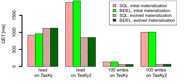
Figure 8: Overhead of generated code.

Wikimedia: Even long evolutions can be easily modeled with BiDEL. To show this, we implement $171$ schema versions of the Wikimedia [7], so data that is written in any of these schema versions, is also visible in all $170$ other schema versions. BiDEL proved to be capable of providing the database schema in each version exactly according to the benchmark and migrating the data accordingly. In Table 4, we summarize how often each SMO has been used in the 211 SMOs long evolution. Even though simple SMOs, like adding and removing tables/columns, are clearly dominating—probably due to the restricted database evolution support of current DBMSes—there are more complex evolutions including the other SMOs as well. Hence, there is a need for more sophisticated database evolution support and BiDEL shows to be feasible.

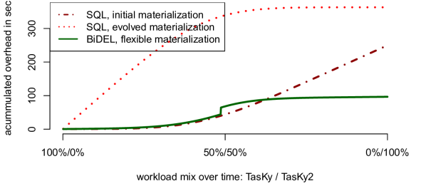
Figure 9: Flexible materialization.

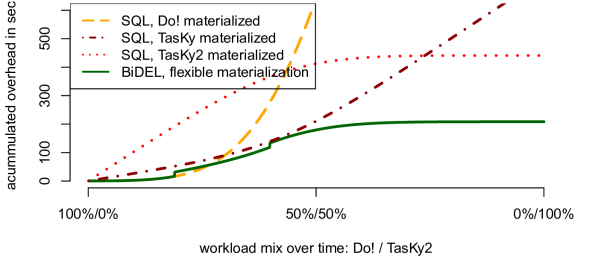
Figure 10: Flexible materialization.

8.2 Overhead of Generated Delta Code

InVerDa’s delta code is generated from Datalog rules and aims at a general and solid solution. So far, our focus is on the correct propagation of data access on multiple co-existing schema versions. We expect the database optimizer to find a fast execution plan, however, there will be an overhead of InVerDa compared to hand-optimized SQL.

TasKy: In Figure 8, we use the previously presented TasKy example with $100\,000$ tasks and compare the performance of InVerDa generated delta code to the handwritten one. There are two aspects to observe. First, the hand-optimized delta code causes slightly less (up to $4\text{\,}\%$) overhead than the generated one. Considering the difference in length and complexity of the code ($359\text{\,}\mathrm{x}$ LOC for the evolution), a performance overhead of $4\text{\,}\%$ in average is more than reasonable for most users. Second, the materialization significantly influences the actual performance. Reading the data in the materialized version is up to twice as fast as accessing it from the respective other version in this scenario. For the write workload (insert new tasks), we observe again a reasonably small overhead compared to handwritten SQL. Interestingly, the evolved materialization is always faster because the initial materialization requires to manage an additional auxiliary table for the foreign key relationship. A DBA can optimize the overall performance for a given workload by adapting the materialization, which is a very simple task with InVerDa. An advisor tool supporting the optimization task is very well imaginable, but out of scope for this paper.

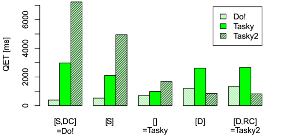
(a) Materializations for TasKy Mix.

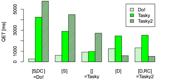
(b) Materializations for TasKy Read.

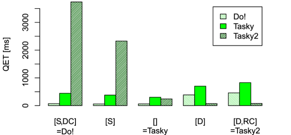
(c) Materializations for TasKy Write.

Figure 11: Different workloads on all possible materialization of TasKy.

8.3 Benefit of Flexible Materialization

Adapting the physical table schema to the current workload is hard with handwritten SQL, but almost for free with InVerDa ($1$ LOC instead of $182$ in our TasKy example). Let’s assume a development team spares the effort for rewriting delta code and works with a fixed materialization.

TasKy: Again, we use the TasKy example with $100\,000$ tasks. Figure 9 shows the accumulated propagation overhead for handwritten SQL with the two fixed materializations and for InVerDa with an adaptive materialization. Assume, over time the workload changes from $0\text{\,}\%$ access to TasKy2 and $100\text{\,}\%$ to TasKy to the opposite $100\text{\,}\%$ and $0\text{\,}\%$ according to the Technology Adoption Life Cycle. The adoption is divided into $1000$ time slices where $1000$ queries are executed respectively. The workload mixes $50\text{\,}\%$ reads, $20\text{\,}\%$ inserts, $20\text{\,}\%$ updates, and $10\text{\,}\%$ deletes. As soon as the evolved materialization is faster for the current workload mix, we instruct InVerDa to change the materialization. As can be seen, InVerDa facilitates significantly better performance—including migration cost—than a fixed materialization.

This effect increases with the length of the evolution, since InVerDa can also materialize intermediate stages of the evolution history. Assume, all users use exclusively the mobile phone app Do!; but as TasKy2 gets released users switch to TasKy2 which comes with its own mobile app. In Figure 10, we simulate the accumulated overhead for either materializing one of the three schema versions or for a flexible materialization. The latter starts at Do!, moves to TasKy after several users started using TasKy2, and finally moves to TasKy2 when the majority of users did so. Again, InVerDa’s flexible materialization significantly reduces the overhead for data propagation without any interaction of a developer.

The DBA can choose between multiple materialization schemas. The number of valid materialization schemas greatly depends on the actual structure of the evolution. The lower bound is a linear sequence of depending SMOs, e.g. one table with $N$ ADD COLUMN SMOs has $N$ valid materializations. The upper bound are $N$ independent SMOs, each evolving another table, with $2^{N}$ valid materializations. Specifically, the TasKy example has five valid materializations.

Figure 11 shows the data access performance on the three schema versions for each of the five materialization schema. The materialization schemas are represented as the lists of SMOs that are materialized. We use abbreviations for SMOs: e.g. $[D,RC]$ on the very right corresponds to schema version TasKy2 since both the decompose SMO (D) and the rename column SMO (RC) are materialized. The initial materialization is in the middle, while e.g. the materialization according to Do! is on the very left. The workload mixes $50\text{\,}\%$ reads, $20\text{\,}\%$ inserts, $20\text{\,}\%$ updates, $10\text{\,}\%$ deletes in Figure 11(a), $100\text{\,}\%$ reads in Figure 11(b), and $100\text{\,}\%$ inserts in Figure 11(c) on the depicted schema versions. Again, the measurements show that accesses to each schema version are fastest when its respective table versions are materialized, i.e. when the physical table schema fits the accessed schema version. However, there are differences in the actual overhead, so the globally optimal materialization depends on the workload distribution among the schema version. E.g. writing to TasKy2 is $49$ times faster when the physical table schema matches TasKy2 instead of Do!. This gain increases with every SMO, so for longer evolutions with more SMOs it will be even higher.

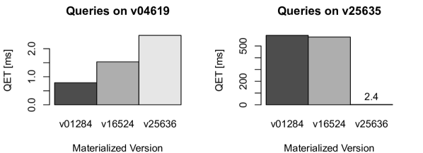
Figure 12: Optimization potential for Wikimedia.

Wikmedia: The benefits of the flexible materialization originate from the increased performance when accessing data locally without the propagation through SMOs. We load our Wikimedia with the data of Akan Wiki in schema version v16524 (109th version) with $14\,359$ pages and $536\,283$ links. We measure the read performance for the template queries from [7] both in schema version v04619 (28th version) and v25635 (171th version). The chosen materializations match version v01284 (1st), v16524 (109th), and v25635 (171th) respectively. In Figure 12, a great performance difference of up to two orders of magnitude is visible, so there is a huge optimization potential. We attribute this asymmetry to the dominance of add column SMOs, which need an expensive join with an auxiliary table to propagate data forwards, but only in a cheap projection to propagate backwards.

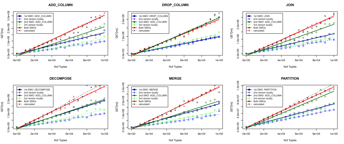
Figure 13: Scaling behavior of the ADD COLUMN SMO.

All possible evolutions with two SMOs: To show that it is always possible to gain a better performance by optimizing the materialization, we conduct a micro benchmark on all possible evolutions with two SMOs—except of creating and dropping tables as well as renaming columns and tables, since they have no relevant performance overhead in the first place. We show that there is always a performance benefit when accessing data locally compared to propagating it through SMOs and we disprove that InVerDa might add complexity to the data access, so two SMOs do not impact each other negatively. We generate evolutions with two SMOs and three schema versions: 1st version – 1st SMO – 2nd version – 2nd SMO – 3rd version. The second version always contains a table $R(a,b,c)$; the number of generated tuples in this table is the x-axis of the charts. In Figure 13, we exemplarily consider all the combinations with add column as 2nd SMO, since this is the most common one. Again, accessing data locally is up to twice as fast as propagating it through an SMO, so the optimization potential exists in all scenarios. The average speedup over all SMOs is $2.1\text{\,}$. We calculate the expected performance for the combination of both SMOs as the sum of both query execution times minus reading data locally at the 2nd schema version. This is reasonable since the data for the 2nd SMO is already in memory after executing the 1st one. Figure 13 shows that the measured time for propagating the data through two SMOs is always in the same range as the calculated combination of the overhead of the two SMOs individually, so we showed that there is great optimization potential for all combinations of those SMOs and we can safely use it without fearing additional overhead when combining SMOs. This holds for all pairs of SMOs: on average the measured time differs only $6.3\text{\,}\%$ from the calculated one. In sum, InVerDa enables the DBA to easily adapt the materialization schema to a changing workload and to significantly speed up query processing without hitting other stakeholders’ interests.

9 Related Work

Both the database evolution [14] and co-existing schema versions [16] are well recognized in database research. For database evolution, existing approaches increase comfort and efficiency, for instance by defining a schema evolution aware query language [15] or by providing a general framework to describe database evolution in the context of evolving applications [8]. With Meta Model Management 2.0 [3], Phil Bernstein et al. introduced a comprehensive tooling to i.a. match, merge, and diff given schema versions. The resulting mappings couple the evolution of both the schema and the data just as our SMOs do; however, the difference is that mappings are derived from given schema versions while InVerDa takes developer-specified mappings and derives the new schema version. Currently, PRISM [5] appears to provide the most advanced database evolution tool with an SMO-based DEL. PRISM was introduced in 2008 and focused on the plain database evolution [6]. Later, PRISM++ added constraint evolution and update rewriting [5].

These existing works provide a great basis for database evolution and InVerDa builds upon them to add logical data independence and co-existence of schema versions, which basically requires bidirectional transformations [17]. Particularly, symmetric relational lenses lay a foundation to describe read and write accesses along a bidirectional mapping [11]. For InVerDa, we adapt this idea to bidirectional SMOs. Another extension of PRISM++ takes a first step towards co-existing schema versions by answering queries on former schema versions w.r.t. to the current data [13], however, InVerDa also covers write operations on those former schema versions. There are multiple systems also taking this step, however, the DELs are usually rather limited or work on different meta models like data warehouses [1]. The ScaDaVer system [18] allows additive and subtractive SMOs on the relational model, which simplifies bidirectionality and hence it is a great starting point towards more powerful DELs. BiDEL also covers restructuring SMOs and is based on established DELs [5, 9]. To the best of our knowledge, we are the first to realize end-to-end support for co-existing schema versions based on such powerful DELs.

10 Conclusions

Current DBMSes do not support co-existing schema versions properly, forcing developers to manually write complex and error-prone delta code, which propagates read/write accesses between schema versions. Moreover, this delta code needs to be adapted manually whenever the DBA changes the physical table schema. InVerDa greatly simplifies creating and maintaining co-existing schema versions for developers, while the DBA can freely change the physical table schema. For this sake, we have introduced BiDEL, an intuitive bidirectional database evolution language that carries enough information to generate all the delta code automatically. We have formally validated BiDEL’s bidirectionality making it a sound and robust basis for InVerDa. In our evaluation, we have shown that BiDEL scripts are significantly shorter than handwritten SQL scripts ($359\text{\,}\mathrm{x}$). The performance overhead caused by the automatically generated delta code is very low but the freedom to easily change the physical table schema is highly valuable: we can greatly speed up query processing by matching the physical table schema to the current workload. In sum, InVerDa finally enables agile—but also robust and maintainable—software development for information systems. Future research topics are (1) zero-downtime migrations, (2) efficient physical table schemas e.g. with redundancy, (3) self-managed DBMSes continuously adapting the physical table schema to the current workload, and (4) optimized delta code within a database system instead of triggers.

Appendix A Bidirectionality of Split

In this paper (Section 5), we merely showed one of the two bidirectionality conditions for the SPLIT SMO to explain the concept. As a reminder, the two conditions are:

$$D_{tgt} =\gamma_{tgt}^{data}(\gamma_{src}(D_{tgt}))$$ (57)

$$D_{src} =\gamma_{src}^{data}(\gamma_{tgt}(D_{src}))$$ (58)

We have already shown Condition 58, so we do the same for Condition 57, now.

Writing data $R_{D}$ and $S_{D}$ from the target-side to the source-side is done with the mapping $\gamma_{src}(R_{D},S_{D})$. With source-side materialization all target-side auxiliary tables are not required, so we apply Lemma 2 to obtain:

$$\mathbf{\gamma_{src}(R_{D},S_{D}):}$$

$$T(p,A)\leftarrow R_{D}(p,A)$$ (59)

$$T(p,A)\leftarrow S_{D}(p,A),\neg R_{D}(p,\_)$$ (60)

$$R^{-}(p)\leftarrow S_{D}(p,A),\neg R_{D}(p,\_),c_{R}(A)$$ (61)

$$R^{*}(p)\leftarrow R_{D}(p,A),\neg c_{R}(A)$$ (62)

$$S^{+}(p,A)\leftarrow S_{D}(p,A),R_{D}(p,A^{\prime}),A\neq A^{\prime}$$ (63)

$$S^{-}(p)\leftarrow R_{D}(p,A),\neg S_{D}(p,\_),c_{S}(A)$$ (64)

$$S^{*}(p)\leftarrow S_{D}(p,A),\neg c_{S}(A)$$ (65)

Reading the target-side data back from the source-side adds the rule set $\gamma_{tgt}$ (Rule 12–17) to the mapping. Using Lemma 1, the mapping $\gamma_{tgt}(\gamma_{src}(T_{D}))$ extends to:

$$\mathbf{\gamma_{tgt}(\gamma_{src}} \mathbf{(R_{D},S_{D})):}$$

$$R(p,A)\leftarrow R_{D}(p,A),c_{R}(A),\neg S_{D}(p,\_)$$ (66)

$$R(p,A)\leftarrow R_{D}(p,A),c_{R}(A),R_{D}(p,\_)$$ (67)

$$R(p,A)\leftarrow R_{D}(p,A),c_{R}(A),S_{D}(p,A^{\prime}),\neg c_{R}(A^{\prime})$$ (68)

$$R(p,A)\leftarrow R_{D}(p,A),R_{D}(p,A),\neg c_{R}(A)$$ (69)

$$R(p,A)\leftarrow \mathbf{S_{D}(p,A)},\neg R_{D}(p,\_),c_{R}(A),\mathbf{\neg S_{D}(p,A)}$$ (70)

$$R(p,A)\leftarrow S_{D}(p,A),\mathbf{\neg R_{D}(p,\_)},c_{R}(A),\mathbf{R_{D}(p,\_)}$$ (71)

$$R(p,A)\leftarrow S_{D}(p,A),\neg R_{D}(p,\_),\mathbf{c_{R}(A)},\mathbf{\neg c_{R}(A)}$$ (72)

$$R(p,A)\leftarrow S_{D}(p,A),\mathbf{\neg R_{D}(p,\_)},\mathbf{R_{D}(p,A)},\neg c_{R}(A)$$ (73)

$$S(p,A)\leftarrow \mathbf{R_{D}(p,A)},c_{S}(A),\mathbf{\neg R_{D}(p,A)},\neg S_{D}(p,\_)$$ (74)

$$S(p,A)\leftarrow \mathbf{R_{D}(p,A)},c_{S}(A),\mathbf{\neg R_{D}(p,A)},\neg R_{D}(p,\_)$$ (75)

$$S(p,A)\leftarrow \mathbf{R_{D}(p,A)},c_{S}(A),\mathbf{\neg R_{D}(p,A)},$$

$$S_{D}(p,A^{\prime}),R_{D}(p,A),A^{\prime}=A$$ (76)

$$S(p,A)\leftarrow R_{D}(p,A),c_{S}(A),\mathbf{S_{D}(p,\_)},\mathbf{\neg S_{D}(p,\_)}$$ (77)

$$S(p,A)\leftarrow \mathbf{R_{D}(p,A)},c_{S}(A),S_{D}(p,\_),\mathbf{\neg R_{D}(p,\_)}$$ (78)

$$S(p,A)\leftarrow R_{D}(p,A),c_{S}(A),S_{D}(p,\_),$$

$$S_{D}(p,A^{\prime}),R_{D}(p,A),A^{\prime}=A$$ (79)

$$S(p,A)\leftarrow R_{D}(p,A),\mathbf{c_{S}(A)},\mathbf{\neg c_{S}(A)},\neg S_{D}(p,\_)$$ (80)

$$S(p,A)\leftarrow R_{D}(p,A),\mathbf{c_{S}(A)},\mathbf{\neg c_{S}(A)},\neg R_{D}(p,A)$$ (81)

$$S(p,A)\leftarrow R_{D}(p,A),\mathbf{c_{S}(A)},\mathbf{\neg c_{S}(A)},$$

$$S_{D}(p,A^{\prime}),R_{D}(p,A),A^{\prime}=A$$ (82)

$$S(p,A)\leftarrow \mathbf{S_{D}(p,A)},\neg R_{D}(p,\_),c_{S}(A),\neg R_{D}(p,\_),$$

$$\mathbf{\neg S_{D}(p,\_)}$$ (83)

$$S(p,A)\leftarrow S_{D}(p,A),\neg R_{D}(p,\_),c_{S}(A),\neg R_{D}(p,\_),$$

$$\neg R_{D}(p,\_)$$ (84)

$$S(p,A)\leftarrow S_{D}(p,A),\mathbf{\neg R_{D}(p,\_)},c_{S}(A),\neg R_{D}(p,\_),$$

$$S_{D}(p,A),\mathbf{R_{D}(p,A^{\prime\prime})},A=A^{\prime\prime}$$ (85)

$$S(p,A)\leftarrow \mathbf{S_{D}(p,A)},\neg R_{D}(p,\_),c_{S}(A),S_{D}(p,\_),$$

$$\mathbf{\neg S_{D}(p,\_)}$$ (86)

$$S(p,A)\leftarrow S_{D}(p,A),\neg R_{D}(p,\_),c_{S}(A),S_{D}(p,\_),$$

$$\neg R_{D}(p,\_)$$ (87)

$$S(p,A)\leftarrow S_{D}(p,A),\mathbf{\neg R_{D}(p,\_)},c_{S}(A),S_{D}(p,\_),$$

$$S_{D}(p,A),\mathbf{R_{D}(p,A^{\prime\prime})},A=A^{\prime\prime}$$ (88)

$$S(p,A)\leftarrow \mathbf{S_{D}(p,A)},\neg R_{D}(p,\_),c_{S}(A),R_{D}(p,A^{\prime}),$$

$$c_{S}(A^{\prime}),\mathbf{\neg S_{D}(p,\_)}$$ (89)

$$S(p,A)\leftarrow S_{D}(p,A),\mathbf{\neg R_{D}(p,\_)},c_{S}(A),\mathbf{R_{D}(p,A^{\prime})},$$

$$c_{S}(A^{\prime}),\neg R_{D}(p,\_)$$ (90)

$$S(p,A)\leftarrow S_{D}(p,A),\mathbf{\neg R_{D}(p,\_)},c_{S}(A),\mathbf{R_{D}(p,A^{\prime})},$$

$$c_{S}(A^{\prime}),S_{D}(p,A),R_{D}(p,A^{\prime\prime}),A=A^{\prime\prime}$$ (91)

$$S(p,A)\leftarrow S_{D}(p,A),R_{D}(p,A^{\prime}),A\neq A^{\prime}$$ (92)

$$S(p,A)\leftarrow R_{D}(p,A),\mathbf{S_{D}(p,A)},\neg c_{S}(A),\mathbf{\neg S_{D}(p,\_)}$$ (93)

$$S(p,A)\leftarrow \mathbf{R_{D}(p,A)},S_{D}(p,A),\neg c_{S}(A),\mathbf{\neg R_{D}(p,\_)}$$ (94)

$$S(p,A)\leftarrow R_{D}(p,A),S_{D}(p,A),\neg c_{S}(A),$$

$$S_{D}(p,A),R_{D}(p,A),A=A$$ (95)

$$S(p,A)\leftarrow \mathbf{S_{D}(p,A)},\neg R_{D}(p,\_),S_{D}(p,A),\neg c_{S}(A),$$

$$\mathbf{\neg S_{D}(p,\_)}$$ (96)

$$S(p,A)\leftarrow S_{D}(p,A),\neg R_{D}(p,\_),S_{D}(p,A),\neg c_{S}(A),$$

$$\neg R_{D}(p,\_)$$ (97)

$$S(p,A)\leftarrow S_{D}(p,A),\mathbf{\neg R_{D}(p,\_)},S_{D}(p,A),\neg c_{S}(A),$$

$$S_{D}(p,A),\mathbf{R_{D}(p,A^{\prime})},A=A^{\prime})$$ (98)

$$T^{\prime}(p,A)\leftarrow \mathbf{R_{D}(p,A)},\neg c_{R}(A),\neg c_{S}(A),\mathbf{\neg R_{D}(p,\_)},$$

$$\neg S_{D}(p,\_)$$ (99)

$$T^{\prime}(p,A)\leftarrow \mathbf{R_{D}(p,A)},\neg c_{R}(A),\neg c_{S}(A),\mathbf{\neg R_{D}(p,\_)},$$

$$S_{D}(p,A^{\prime}),c_{S}(A^{\prime})$$ (100)

$$T^{\prime}(p,A)\leftarrow R_{D}(p,A),\mathbf{\neg c_{R}(A)},\neg c_{S}(A),R_{D}(p,A),$$

$$\mathbf{c_{R}(A)},\neg S_{D}(p,\_)$$ (101)

$$T^{\prime}(p,A)\leftarrow R_{D}(p,A),\mathbf{\neg c_{R}(A)},\neg c_{S}(A),R_{D}(p,A),$$

$$\mathbf{c_{R}(A)},S_{D}(p,A^{\prime\prime}),c_{S}(A^{\prime\prime})$$ (102)

$$T^{\prime}(p,A)\leftarrow \mathbf{S_{D}(p,A)},\neg R_{D}(p,\_),\neg c_{R}(A),\neg c_{S}(A),$$

$$\neg R_{D}(p,\_),\mathbf{\neg S_{D}(p,\_)}$$ (103)

$$T^{\prime}(p,A)\leftarrow S_{D}(p,A),\neg R_{D}(p,\_),\neg c_{R}(A),\mathbf{\neg c_{S}(A)},$$

$$\neg R_{D}(p,\_),S_{D}(p,A),\mathbf{c_{S}(A)})$$ (104)

$$T^{\prime}(p,A)\leftarrow \mathbf{S_{D}(p,A)},\neg R_{D}(p,\_),\neg c_{R}(A),\neg c_{S}(A),$$

$$R_{D}(p,A^{\prime}),c_{R}(A^{\prime}),\mathbf{\neg S_{D}(p,\_)}$$ (105)

$$T^{\prime}(p,A)\leftarrow S_{D}(p,A),\mathbf{\neg R_{D}(p,\_)},\neg c_{R}(A),\neg c_{S}(A),$$

$$\mathbf{R_{D}(p,A^{\prime})},c_{R}(A^{\prime}),S_{D}(p,A^{\prime\prime}),c_{S}(A^{\prime\prime})$$ (106)

Using Lemma 4 we remove all rules that have contradicting literals (marked bold). Particularly, there remains no rule for $T^{\prime}$ as expected. Further, we remove duplicate literals within the rules, so we obtain the simplified rule set:

$$R(p,A)\leftarrow R_{D}(p,A),c_{R}(A),\neg S_{D}(p,\_)$$ (107)

$$R(p,A)\leftarrow R_{D}(p,A),c_{R}(A)$$ (108)

$$R(p,A)\leftarrow R_{D}(p,A),c_{R}(A),S_{D}(p,A^{\prime}),\neg c_{R}(A^{\prime})$$ (109)

$$R(p,A)\leftarrow R_{D}(p,A),\neg c_{R}(A)$$ (110)

$$S(p,A)\leftarrow S_{D}(p,A),R_{D}(p,A),c_{S}(A)$$ (111)

$$S(p,A)\leftarrow S_{D}(p,A),\neg R_{D}(p,\_),c_{S}(A)$$ (112)

$$S(p,A)\leftarrow S_{D}(p,A),\neg R_{D}(p,\_),c_{S}(A)$$ (113)

$$S(p,A)\leftarrow S_{D}(p,A),R_{D}(p,A^{\prime}),A\neq A^{\prime}$$ (114)

$$S(p,A)\leftarrow S_{D}(p,A),R_{D}(p,A),\neg c_{S}(A)$$ (115)

$$S(p,A)\leftarrow S_{D}(p,A),\neg R_{D}(p,\_),\neg c_{S}(A)$$ (116)

Rule 111 is derived from Rule 79 by applying the equivalence of $A$ and $A^{\prime}$ to the remaining literals. Let’s now focus on the rules for $R$. Rules 107 and 109 are subsumed by Rule 108, since they contain the identical literals as Rule 108 plus additional conditions. Lemma 3 allows us to further reduce Rules 108 and 110, so we achieve that all tuples in $R$ survive one round trip without any information loss or gain:

$$R(p,A)\leftarrow R_{D}(p,A)$$ (117)

We also reduce the rules for $S$. Rule 113 can be removed, since it is equal to Rule 112. With Lemma 3, Rules 112 and 116 as well as Rules 111 and 115 can be combined respectively. This results in the following rules for $S$:

$$S(p,A)\leftarrow S_{D}(p,A),R_{D}(p,A)$$ (118)

$$S(p,A)\leftarrow S_{D}(p,A),\neg R_{D}(p,\_)$$ (119)

$$S(p,A)\leftarrow S_{D}(p,A),R_{D}(p,A^{\prime}),A\neq A^{\prime}$$ (120)

Rules 118 and 120 basically state that the payload data in $R$ ($A$ and $A^{\prime}$ respectively) is either equal to or different from the payload data in $S$ for the same key $p$. When we rewrite Rule 118 to:

$$S(p,A)\leftarrow S_{D}(p,A),R_{D}(p,A^{\prime}),A=A^{\prime}$$ (121)

we can apply Lemma 3 to obtain the two rules:

$$S(p,A)\leftarrow S_{D}(p,A),R_{D}(p,\_)$$ (122)

$$S(p,A)\leftarrow S_{D}(p,A),\neg R_{D}(p,\_)$$ (123)

With the help of Lemma 3, we reduce $\gamma_{tgt}(\gamma_{src}(R_{D},S_{D}))$ to

$$R(p,A)\leftarrow R_{D}(p,A)$$ (124)

$$S(p,A)\leftarrow S_{D}(p,A)\qed$$ (125)

So, both Condition 57 and Condition 58 for the bidirectionallity of the split SMO are formally validated by now. Since the merge SMO is the inverse of the split SMO and uses the exact same mapping rules vice versa, we also implicitly validated the bidirectionality of the merge SMO. We can now safely say: wherever we materialize the data, the mapping rules always guarantee that each table version can be accessed just like a regular table—no data will be lost or gained. This is a strong guarantee and the basis for InVerDa to provide co-existing schema versions within a single database.

Appendix B Remaining SMOs

We introduce the syntax and semantics of the remaining SMOs from Figure 2. Further, we include the results of the formal evaluation of their bidirectionality. Please note that creating, dropping, and renaming tables as well as renaming columns exclusively affects the schema version catalog and does not include any kind of data evolution, hence there is no need to define mapping rules for these SMOs. In Section B.1, we introduce the ADD COLUMN SMO. Since SMOs are bidirectional, exchanging the rule sets $\gamma_{src}$ and $\gamma_{tgt}$ yields the inverse SMO: DROP COLUMN. There are different extends for the JOIN and its inverse DECOMPOSE SMO: a join can have inner or outer semantics and it can be done based on the primary key, a foreign key, or on an arbitrary condition. As summarized in Table 5, each configuration requires different mapping functions, however some are merely the inverse or variants of others. The inverse of DECOMPOSE is OUTER JOIN and joining at a foreign key is merely a specific condition.

B.1 Add Column / Drop Column

SMO: ADD COLUMN $b$ AS $f$($r_{1}$,…,$r_{n}$) INTO $R$
Inverse: DROP COLUMN $b$ FROM $R$ DEFAULT $f$($r_{1}$,…,$r_{n}$)
The ADD COLUMN SMO adds a new column $b$ to a table $R$ and calculates the new values for $b$ according to the given function $f$. The inverse DROP COLUMN SMO uses the same parameters to ensure bidirectionality.

$$\mathbf{\gamma_{tgt}:}\hskip 8.53581ptR^{\prime}(p,A,b) \leftarrow R(p,A),b=f_{B}(p,A),\neg B(p,\_)$$ (126)

$$R^{\prime}(p,A,b) \leftarrow R(p,A),B(p,b)$$ (127)

$$\mathbf{\gamma_{src}:}\hskip 19.06332ptR(p,A) \leftarrow R^{\prime}(p,A,\_)$$ (128)

$$B(p,b) \leftarrow R^{\prime}(p,\_,b)$$ (129)

$$\mathbf{\gamma_{src}(\gamma_{tgt}(R_{D})):}$$

$$R(p,A) \leftarrow R_{D}(p,A)$$ (130)

$$B(p,b) \leftarrow R_{D}(p,A),b=f_{B}(p,A)\qed$$ (131)

$$\mathbf{\gamma_{tgt}(\gamma_{src}(R_{D}^{\prime})):}$$

$$R^{\prime}(p,A,b) \leftarrow R_{D}^{\prime}(p,A,b)\qed$$ (132)

The auxiliary table $B$ stores the values of the new column when the SMO is virtualized to ensure bidirectionality. With the projection to data tables, the SMO satisfies Conditions 57 and 58. For repeatable reads, the table $B$ is also needed when data is given in the source schema version (Rule 131).

B.2 Decompose on the Primary Key

SMO: DECOMPOSE TABLE $R$ INTO $S$($A$), $T$($B$) ON PK
Inverse: OUTER JOIN TABLE $S$, $T$ INTO $R$ ON PK
To fill the gaps potentially resulting from the inverse outer join, we use the null value $\omega_{R}$. The bidirectionality conditions are satisfied: after one round trip, no data is lost or gained.

$$\mathbf{\gamma_{tgt}:}\hskip 62.59605ptS(p,A) \leftarrow R(p,A,\_),A\neq\omega_{R}$$ (133)

$$T(p,B) \leftarrow R(p,\_,B),B\neq\omega_{R}$$ (134)

$$\mathbf{\gamma_{src}:}\hskip 49.79231ptR(p,A,B) \leftarrow S(p,A),T(p,B)$$ (135)

$$R(p,A,\omega_{R}) \leftarrow S(p,A),\neg T(p,\_)$$ (136)

$$R(p,\omega_{R},B) \leftarrow\neg S(p,\_),T(p,B)$$ (137)

$$\mathbf{\gamma_{src}(\gamma_{tgt}(R_{D})):}\hskip 5.69054ptR(p,A,B) \leftarrow R_{D}(p,A,B)\qed$$ (138)

$$\mathbf{\gamma_{tgt}(\gamma_{src}(S_{D},T_{D})):}S(p,A) \leftarrow S_{D}(p,A)$$ (139)

$$T(p,B) \leftarrow T_{D}(p,B)\qed$$ (140)

	Decompose	Outer Join	Inner Join
ON PK	B.2	Inverse of B.2	B.5
ON FK	B.3	Inverse of B.3	Variant of B.6
ON Cond.	B.4	Inverse of B.4	B.6

Table 5: Overview of different Decompose and Join SMOs.

B.3 Decompose on a Foreign Key

SMO: DECOMPOSE TABLE $R$ INTO $S$($A$), $T$($B$) ON FK $t$
Inverse: OUTER JOIN TABLE $S$, $T$ INTO $R$ ON FK $t$
A DECOMPOSE, which creates a new foreign key, needs to generate new identifiers. Assume we cut away the addresses from persons stored in one table, we eliminate all duplicates in the new address table, assign a new identifier to each address, and finally add a foreign key column to the new persons table. On every call, the function $id_{T}(B)$ returns a new unique identifier for the payload data $B$ in table $T$. In our implementation, this is merely a regular SQL sequence and the mapping rules ensure that an already generated identifier is reused for the same data. In order to guarantee proper evaluation of these functions, we enforce a sequential evaluation of the rules by distinguishing between existing and new data. For a literal $L$, we use the indexes $L_{o}$ (old) and $L_{n}$ (new) to note the difference, however they have now special semantics and are evaluated like any other literal in Datalog. For a DECOMPOSE ON FK, we propose the rule set:

$$\mathbf{\gamma_{tgt}:}$$

$$T_{n}(t,B) \leftarrow R(p,\_,B),ID_{R}(p,t)$$ (141)

$$T_{n}(t,B) \leftarrow R(p,\_,B),\neg ID_{R}(p,t),$$

$$\phantom{\leftarrow}\neg T_{o}(\_,B),t=id_{T}(B)$$ (142)

$$T_{n}(t,B) \leftarrow R(\_,\_,B),T_{o}(t,B)$$ (143)

$$S(p,A,t) \leftarrow R(p,A,\_),ID_{R}(p,t)$$ (144)

$$S(p,A,\omega) \leftarrow R(p,A,\_),ID_{R}(p,\omega)$$ (145)

$$S(p,A,t) \leftarrow R(p,A,B),\neg ID_{R}(p,\_),T_{n}(t,B)$$ (146)

$$\mathbf{\gamma_{src}:}$$

$$R(p,A,B) \leftarrow S(p,A,t),T(t,B)$$ (147)

$$R(p,A,\omega) \leftarrow S(p,A,\omega)$$ (148)

$$R(t,\omega,B) \leftarrow\neg S(\_,\_,t),T(t,B)$$ (149)

$$ID_{R}(p,t) \leftarrow S(p,\_,t),T(t,\_)$$ (150)

$$ID_{R}(p,\omega) \leftarrow S(p,\_,\omega)$$ (151)

$$ID_{R}(t,t) \leftarrow\neg S(\_,\_,t),T(t,\_)$$ (152)

$$\mathbf{\gamma_{src}(\gamma_{tgt}(R_{D})):}$$

$$R(p,A,B) \leftarrow R_{D}(p,A,B)$$ (153)

$$ID_{R}(p,t) \leftarrow R_{D}(p,A,B),t=id_{T}(B)\qed$$ (154)

$$\mathbf{\gamma_{tgt}(\gamma_{src}(S_{D},T_{D})):}$$

$$T(t,B) \leftarrow T_{D}(t,B)$$ (155)

$$S(p,A,t) \leftarrow S_{D}(p,A,t)\qed$$ (156)

Projecting the outcomes to the data tables, again satisfies our bidirectionality Conditions 57 and 58. Hence, no matter whether the SMO is virtualized or materialized, both the source and the target side behave like common single-schema databases. Storing data in $R$ implicitly generates new values to the auxiliary table $ID_{R}$, which is intuitive: we need to store the assigned identifiers for the target version to ensure repeatable reads on those generated identifiers.

B.4 Decompose on Condition

SMO: DECOMPOSE TABLE $R$ INTO $S$($A$), $T$($B$) ON $c(A,B)$
Inverse: OUTER JOIN TABLE $S$, $T$ INTO $R$ ON $c(A,B)$
To e.g. normalize a table that holds books and authors ($N:M$), we can either use two subsequent DECOMPOSE ON FK to maintain the relationship between books and authors, or—if the new evolved version just needs the list of authors and the list of books—we simply split them giving up the relationship. In the following, we provide rules for the latter case. Either way we have to generate new identifiers for both the books and the authors. We use the same identity generating function as in Section B.3.

$$\mathbf{\gamma_{tgt}:}$$

$$S_{n}(s,A)\leftarrow R(r,A,\_),ID_{o}(r,s,\_)$$ (157)

$$S_{n}(s,A)\leftarrow R(r,A,\_),\neg ID_{o}(r,\_,\_),$$

$$A\neq\omega_{R},s=id_{S}(A)$$ (158)

$$S_{n}(r,A)\leftarrow R(r,A,\_),\neg ID_{o}(r,\_,\_),A=\omega_{R}$$ (159)

$$T_{n}(t,B)\leftarrow R(r,\_,B),ID_{o}(r,\_,t)$$ (160)

$$T_{n}(t,B)\leftarrow R(r,\_,B),\neg ID_{o}(r,\_,\_),$$

$$B\neq\omega_{R},t=id_{T}(B)$$ (161)

$$T_{n}(r,B)\leftarrow R(r,\_,B),\neg ID_{o}(r,\_,\_),B=\omega_{R}$$ (162)

$$ID_{n}(r,s,t)\leftarrow R(r,A,B),S_{n}(s,A),T_{n}(t,B)$$ (163)

$$R^{-}(s,t)\leftarrow \neg R(\_,A,B),S_{n}(s,A),$$

$$T_{n}(t,B),c(A,B)$$ (164)

$$\mathbf{\gamma_{src}:}$$

$$R_{o}(r,A,B)\leftarrow S(s,A),T(t,B),ID_{o}(r,s,t)$$ (165)

$$R_{o}(r,A,B)\leftarrow S(s,A),T(t,B),c(A,B),\neg R^{-}(s,t),$$

$$\neg ID_{o}(\_,s,t),r=id_{R}(A,B)$$ (166)

$$ID_{n}(r,s,t)\leftarrow S(s,A),T(t,B),c(A,B),R_{o}(r,A,B)$$ (167)

$$ID_{n}(r,s,t)\leftarrow ID_{o}(r,s,t)$$ (168)

$$R_{n}(r,A,B)\leftarrow R_{o}(r,A,B)$$ (169)

$$R_{n}(s,A,\omega_{R})\leftarrow S(s,A),\neg ID_{n}(\_,s,\_)$$ (170)

$$R_{n}(t,\omega_{R},B)\leftarrow T(t,B),\neg ID_{n}(\_,\_,t)$$ (171)

$$\mathbf{\gamma_{src}(\gamma_{tgt}(S_{D},T_{D})):}$$

$$R_{n}(r,A,B)\leftarrow R_{D}(r,A,B)$$ (172)

$$ID_{n}(r,s,t)\leftarrow R_{D}(r,A,B),$$

$$s=id_{S}(A),t=id_{T}(B)\qed$$ (173)

$$\mathbf{\gamma_{tgt}(\gamma_{src}(R_{D})):}$$

$$S(s,A)\leftarrow S_{D}(s,A)$$ (174)

$$T(t,B)\leftarrow T_{D}(t,B)$$ (175)

$$ID(r,s,t)\leftarrow S_{D}(s,A),T_{D}(t,B),$$

$$c(A,B),r=id_{R}(A,B)\qed$$ (176)

The bidirectionality Conditions 57 and 58 are satisfied. For repeatable reads, the auxiliary table $ID$ stores the generated identifiers independently of the chosen materialization.

B.5 Inner Join on Primary Key

SMO: JOIN TABLE $R$, $S$ INTO $T$ ON PK
For this join, we merely need one auxiliary table to store those tuples that do not match with a join partner. Since both bidirectionality conditions hold in the end, we have formally shown the bidirectionality of JOIN ON PK.

$$\mathbf{\gamma_{tgt}:}\hskip 51.21495ptR(p,A,B) \leftarrow S(p,A),T(p,B)$$ (177)

$$S^{+}(p,A) \leftarrow S(p,A),\neg T(p,\_)$$ (178)

$$T^{+}(p,B) \leftarrow\neg S(p,\_),T(p,B)$$ (179)

$$\mathbf{\gamma_{src}:}\hskip 62.59605ptS(p,A) \leftarrow R(p,A,\_)$$ (180)

$$S(p,A) \leftarrow S^{+}(p,A)$$ (181)

$$T(p,B) \leftarrow R(p,\_,B)$$ (182)

$$T(p,B) \leftarrow T^{+}(p,B)$$ (183)

$$\mathbf{\gamma_{src}(\gamma_{tgt}(S_{D},T_{D})):}S(p,A) \leftarrow S_{D}(p,A)$$ (184)

$$T(p,B) \leftarrow T_{D}(p,B)\qed$$ (185)

$$\mathbf{\gamma_{tgt}(\gamma_{src}(R_{D})):}\hskip 4.2679ptR(p,A,B) \leftarrow R_{D}(p,A,B)\qed$$ (186)

B.6 Inner Join on Condition

SMO: JOIN TABLE $R$, $S$ INTO $T$ ON $c(A,B)$
A join on a condition creates new tuples, so we have to generate new identifiers as well. We use the notion introduced in Section B.3 and satisfy the bidirectionality conditions.

$$\mathbf{\gamma_{tgt}:}$$

$$R_{n}(r,A,B)\leftarrow S(s,A),T(t,B),ID_{o}(r,s,t)$$ (187)

$$R_{n}(r,A,B)\leftarrow S(s,A),T(t,B),c(A,B),\neg R^{-}(s,t),$$

$$\neg ID_{o}(\_,s,t),r=id_{R}(A,B)$$ (188)

$$ID_{n}(r,s,t)\leftarrow S(s,A),T(t,B),c(A,B),R_{n}(r,A,B)$$ (189)

$$ID_{n}(r,s,t)\leftarrow ID_{o}(r,s,t)$$ (190)

$$S^{+}(s,A)\leftarrow S(s,A),\neg ID_{n}(\_,s,\_)$$ (191)

$$T^{+}(t,B)\leftarrow T(t,B),\neg ID_{n}(\_,\_,t)$$ (192)

$$\mathbf{\gamma_{src}:}$$

$$S_{n}(s,A)\leftarrow R(r,A,\_),ID(r,s,\_)$$ (193)

$$S_{n}(s,A)\leftarrow R(r,A,\_),\neg ID(r,s,\_),s=id_{S}(A)$$ (194)

$$S_{n}(s,A)\leftarrow S^{+}(s,A)$$ (195)

$$T_{n}(t,B)\leftarrow R(r,\_,B),ID(r,\_,t)$$ (196)

$$T_{n}(t,B)\leftarrow R(r,\_,B),\neg ID(r,\_,t),t=id_{T}(B)$$ (197)

$$T_{n}(t,B)\leftarrow T^{+}(t,B)$$ (198)

$$ID(r,s,t)\leftarrow R(r,A,B),S_{n}(s,A),T_{n}(t,B)$$ (199)

$$R^{-}(s,t)\leftarrow \neg R(\_,A,B),S_{n}(s,A),T_{n}(t,B),c(A,B)$$ (200)

$$\mathbf{\gamma_{src}(\gamma_{tgt}(S_{D},T_{D})):}$$

$$S(s,A)\leftarrow S_{D}(s,A)$$ (201)

$$T(t,B)\leftarrow T_{D}(t,B)$$ (202)

$$ID(r,s,t)\leftarrow S_{D}(s,A),T_{D}(t,B),$$

$$c(A,B),r=id_{R}(A,B)\qed$$ (203)

$$\mathbf{\gamma_{tgt}(\gamma_{src}(R_{D})):}$$

$$R_{n}(r,A,B)\leftarrow R_{D}(r,A,B)$$ (204)

$$ID_{n}(r,s,t)\leftarrow R_{D}(r,A,B),$$

$$s=id_{S}(A),t=id_{T}(B)\qed$$ (205)

In sum, BiDEL’s SMOs are formally guaranteed to be bidirectional: a solid ground for co-existing schema versions.

References

- [1] M. Arora and A. Gosain. Article: Schema Evolution for Data Warehouse: A Survey. International Journal of Computer Applications, 22(5):6–14, 2011.
- [2] A. Behrend, U. Griefahn, H. Voigt, and P. Schmiegelt. Optimizing continuous queries using update propagation with varying granularities. In SSDBM ’15, pages 1–12, New York, USA, jun 2015. ACM Press.
- [3] P. A. Bernstein and S. Melnik. Model management 2.0. In Proceedings of the 2007 ACM SIGMOD international conference on Management of data - SIGMOD ’07, page 1, New York, New York, USA, 2007. ACM Press.
- [4] M. L. Brodie and J. T. Liu. Keynote: The Power and Limits of Relational Technology In the Age of Information Ecosystems. In OTM’10, pages 2–3, 2010.
- [5] C. Curino, H. J. Moon, A. Deutsch, and C. Zaniolo. Automating the database schema evolution process. VLDB Journal, 22(1):73–98, dec 2013.
- [6] C. Curino, H. J. Moon, and C. Zaniolo. Graceful database schema evolution: the PRISM workbench. VLDB Endowment, 1(1):761–772, aug 2008.
- [7] C. Curino, L. Tanca, H. J. Moon, and C. Zaniolo. Schema evolution in wikipedia: toward a web information system benchmark. In ICEIS, pages 323–332, 2008.
- [8] E. Domínguez, J. Lloret, Á. L. Rubio, and M. a. Zapata. MeDEA: A database evolution architecture with traceability. Data and Knowledge Engineering, 65(3):419–441, 2008.
- [9] K. Herrmann, H. Voigt, A. Behrend, and W. Lehner. CoDEL - A Relationally Complete Language for Database Evolution. In ADBIS ’15, pages 63–76, Poitiers, France, 2015. Springer.
- [10] K. Herrmann, H. Voigt, T. Seyschab, and W. Lehner. InVerDa – co-existing schema versions made foolproof. In ICDE ’16, pages 1362–1365. IEEE, 2016.
- [11] M. Hofmann, B. Pierce, and D. Wagner. Symmetric lenses. ACM SIGPLAN Notices - POPL ’11, 46(1):371, jan 2011.
- [12] P. Howard. Data Migration Report, 2011.
- [13] H. J. Moon, C. Curino, M. Ham, and C. Zaniolo. PRIMA - archiving and querying historical data with evolving schemas. In SIGMOD ’09, pages 1019–1022. ACM Press, jun 2009.
- [14] E. Rahm and P. a. Bernstein. An online bibliography on schema evolution. ACM SIGMOD Record, 35(4):30–31, dec 2006.
- [15] J. F. Roddick. SQL/SE - A Query Language Extension for Databases Supporting Schema Evolution. ACM SIGMOD Record, 21(2):10–16, sep 1992.
- [16] J. F. Roddick. A survey of schema versioning issues for database systems. Information and Software Technology, 37(7):383–393, 1995.
- [17] J. F. Terwilliger, A. Cleve, and C. Curino. How Clean Is Your Sandbox? Lecture Notes in Computer Science, 7307:1–23, 2012.
- [18] B. Wall and R. Angryk. Minimal data sets vs. synchronized data copies in a schema and data versioning system. In PIKM ’11, page 67, New York, USA, oct 2011. ACM Press.